Spectra of Elliptic Operators on Quantum Graphs with Small Edges

Abstract

We consider a general second order self-adjoint elliptic operator on an arbitrary metric graph, to which a small graph is glued. This small graph is obtained via rescaling a given fixed graph $\gamma$ by a small positive parameter $\epsilon$. The coefficients in the differential expression are varying, and they, as well as the matrices in the boundary conditions, can also depend on $\epsilon$ and we assume that this dependence is analytic. We introduce a special operator on a certain extension of the graph $\gamma$ and assume that this operator has no embedded eigenvalues at the threshold of its essential spectrum. It is known that under such assumption the perturbed operator converges to a certain limiting operator. Our main results establish the convergence of the spectrum of the perturbed operator to that of the limiting operator. The convergence of the spectral projectors is proved as well. We show that the eigenvalues of the perturbed operator converging to limiting discrete eigenvalues are analytic in $\epsilon$ and the same is true for the associated perturbed eigenfunctions. We provide an effective recurrent algorithm for determining all coefficients in the Taylor series for the perturbed eigenvalues and eigenfunctions.

1. Introduction

Spectral properties of elliptic operators on graphs with small edges are of a special interest and attract quite a lot of attention. Small edges is a specific singular geometric perturbation, which can be introduced due to the nature of graphs. One of early results on graphs with small edges was about a model of a woven membrane, see [1,2], which was shown to be approximated by a two-dimensional operator on an Euclidean domain covered by such membrane.

The graphs with finitely many small edges attracted more attention and one of early results stated that that a general vertex condition in a graph can be approximated in the norm resolvent sense via ornamenting by small edges supporting a magnetic field and with delta-coupling at the vertices [3]. An essential progress was made in very recent works [4,5] just few years ago. Here, Schrödinger operators on general graphs with arbitrarily placed small edges were considered. The main obtained result stated that under a certain non-resonance condition, see Condition 3.2 in [4], the perturbed operator converged to a certain limiting operator in the norm resolvent sense and the estimate for the convergence rate was established. The limiting operators was defined on a graph, in which the small edges were replaced by the vertices to which they shrink and at such vertices certain limiting boundary conditions were determined. These results were further developed in [6,7], where a general elliptic operator with varying coefficients was considered on a graph with small edges rescaled by means of a single small parameter. The coefficients in the differential expression and in the boundary conditions were allowed to depend analytically on the same small parameter. It was shown that certain parts of the resolvent of such operator depended analytically in $\epsilon$ and were represented by converging Taylor series. This allowed to represent the perturbed resolvent by a converging Taylor-like series with effective estimates for the remainders.

A next natural question is the behavior of the spectrum. This question was addressed in [4] for the aforementioned Schrödinger operator on a general graph with small edges. The convergence of the spectrum and corresponding spectral projectors was established. In particular, it was shown that the non-resonance condition was important and without it, the convergence of the spectrum could fail. We also mention few recent papers [8,9,10,11], where the resolvents and spectra were studied for some toy models represented by very simple graphs with small edges.

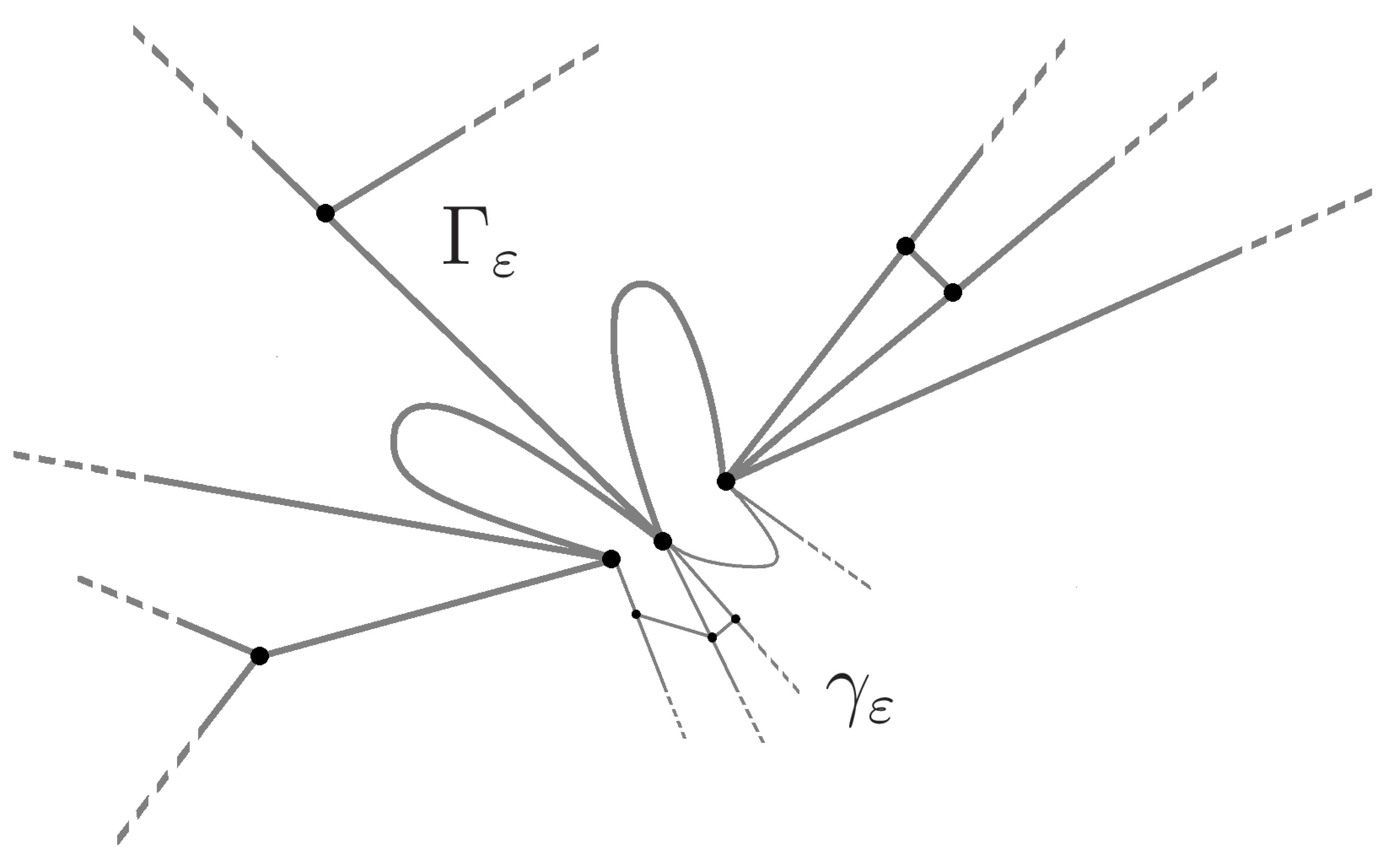
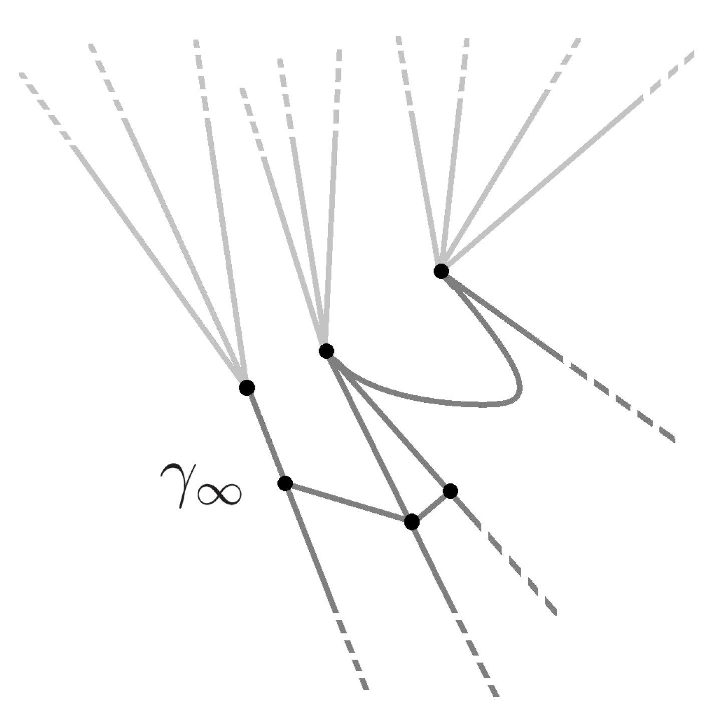
In the present work, we continue studying the model proposed in [6,7]. Namely, we consider a general self-adjoint second order elliptic operator on an arbitrary graph, to which a small graph is glued. The small graph is obtained via rescaling a given fixed graph by a small positive parameter $\epsilon$, see Figure 1 and Figure 2. The coefficients of the differential expression are varying and can additionally depend on $\epsilon$. For the coefficients on fixed edges, this dependence on $\epsilon$ is analytic, while the coefficients on small edges can be even meromorphic. The boundary conditions are of a general matrix form with the matrices analytically depending on $\epsilon$. The limiting operator is known thanks to the results in [6,7]. We show that the spectrum of the perturbed operator converges to that of the limiting operator and we provide an estimate for the distance between these two spectra. We also establish the convergence of the corresponding spectral projectors. Our second main result states that the eigenvalues of the perturbed operator converging to limiting discrete eigenvalues are analytic in $\epsilon$. A similar analyticity property is established for the associated eigenfunctions. We provide an effective recurrent algorithm for determining the coefficients in the Taylor series for both eigenvalues and eigenfunctions. Once the coefficients are found, the sums of the Taylor series are exactly the eigenvalues and the eigenfunctions of the perturbed operator and in this sense, we can say that these eigenvalues and eigenfunctions are found explicitly.

Figure 1. Graph ${\Gamma }_{\epsilon }$ with a glued small graph. The small edges in the graph ${\Gamma }_{\epsilon }$ are indicated by thin lines.

Figure 2. Examples of initial graphs $\Gamma$ and $\gamma$. Here, the edges incident to $M_0$ are split into three groups ($n=3$).

The paper is organized as follows. In the next section, we describe the problem, introduce auxiliary notations, formulate our main results and discuss their main features. The third section is devoted to proving the convergence of the spectrum and of the associated spectral projectors. In the fourth section, we prove the analyticity of the perturbed eigenvalues and the associated eigenfunctions, while in the fifth section, we describe an algorithm for determining the coefficients of their Taylor series.

2. Problem and Main Results

2.1. Problem

Let $\Gamma$ be a finite graph, that is, it contains finitely many vertices and edges. We assume that this graph contains no isolated vertices and edges and is metric, that is, each edge is equipped with a length, direction and a variable on it and on each edge, the usual Lebesgue measure is introduced. The graph $\Gamma$ can contain edges of both finite and infinite lengths.

By $M_0$ we denote an arbitrary vertex in the graph $\Gamma$, while ${\mathrm{e}}_i$, $i=1,\dots ,d_0$, are the edges incident to $M_0$; each possible loop in the family ${\left\{{\mathrm{e}}_i\right\}}_{i=1,\dots ,d_0}$ is counted twice. We introduce one more arbitrary finite metric graph $\gamma$ containing only edges of finite lengths and no isolated vertices or edges, see Figure 2.

We contract the graph $\gamma$ in ${\epsilon }^{-1}$ times, where $\epsilon$ is a small positive parameter, that is, each edge $\mathrm{e}$ in the graph $\gamma$ of a length $\left|\mathrm{e}\right|$ is replaced by an edge of the length $\epsilon \left|\mathrm{e}\right|$, while all vertices remain unchanged. The graph obtained under such contraction is denoted by ${\gamma }_{\epsilon }$.

The graph we study is obtained by gluing the graph ${\gamma }_{\epsilon }$ to $\Gamma$ at the vertex $M_0$. This gluing is defined as follows. First we choose n arbitrary vertices $M_j$, $j=1,\dots ,n$, in the graph ${\gamma }_{\epsilon }$. Using the same number n, we partition the edges ${\mathrm{e}}_i$, $i=1,\dots ,d_0$, of the graph $\Gamma$ into n disjoint non-empty groups ${\left\{{\mathrm{e}}_i\right\}}_{i\in J_j}$, $j=1,\dots ,n$, and replace the vertex $M_0$ in the graph $\Gamma$ by its n copies, one copy for each group ${\left\{{\mathrm{e}}_i\right\}}_{i\in J_j}$. Here, $J_j$ are some disjoint non-empty sets of indices and ${\displaystyle \bigcup _{j=1}^n}{J}_j=\{1,\dots ,d_0\}$, $1⩽n⩽d_0$. The gluing then is made by considering the union of the graphs $\Gamma$ and ${\gamma }_{\epsilon }$ and identifying the vertices $M_j$, $j=1,\dots ,n$, with the aforementioned copies of the vertex $M_0$ in the graph $\Gamma$, see Figure 1. This new graph is denoted by ${\Gamma }_{\epsilon }$. It consists of a fixed part $\Gamma$ and of a small graph ${\gamma }_{\epsilon }$. In the graph ${\Gamma }_{\epsilon }$, the edges $e_i$, $i=1,\dots ,d_0$, are not incident to the same vertex $M_0$. Instead of this, each group ${\left\{{\mathrm{e}}_i\right\}}_{i\in J_j}$ is incident to the vertex $M_j$ in the graph ${\gamma }_{\epsilon }$.

Hereafter, we identify the graphs $\Gamma$ and ${\gamma }_{\epsilon }$ with the corresponding subgraphs in ${\Gamma }_{\epsilon }$. Each function defined on ${\Gamma }_{\epsilon }$ is also supposed to be defined on $\Gamma$ and ${\gamma }_{\epsilon }$ and vice versa. On each edge in $\Gamma$ and $\gamma$ we introduce arbitrarily a direction and an associated variable. The chosen directions then is transferred to the graph ${\Gamma }_{\epsilon }$; the same is done for the variables on the edges in the graph $\Gamma$.

The main object of our study is an operator ${\mathcal{H}}_{\epsilon }$ in $L_2\left({\Gamma }_{\epsilon }\right)$ with the differential expression

$$\begin{array}{c}\widehat{\mathcal{H}}\left(\epsilon \right):=-\frac{d}{dx}{V}_{\epsilon }^{\left(2\right)}\frac{d}{dx}+\mathrm{i}\left(\frac{d}{dx}{V}_{\epsilon }^{\left(1\right)}+V_{\epsilon }^{\left(1\right)}\frac{d}{dx}\right)+V_{\epsilon }^{\left(0\right)},\\ V_{\epsilon }^{\left(i\right)}:=\left\{\begin{array}{cccc}& V_{\Gamma }^{\left(i\right)}(·,\epsilon )\hfill & & \mathrm{on}\Gamma ,\hfill \\ \hfill {\epsilon }^{i-2}& {\mathcal{S}}_{\epsilon }{V}_{\gamma }^{\left(i\right)}(·,\epsilon )\hfill & & \mathrm{on}{\gamma }_{\epsilon }.\hfill \end{array}\right.\end{array}$$

(1)

This expression is defined on each edge of the graph ${\Gamma }_{\epsilon }$ and the symbol x stands for the variable on a considered edge. The symbol $\mathrm{i}$ denotes the imaginary unit, $V_{\Gamma }^{\left(i\right)}=V_{\Gamma }^{\left(i\right)}(·,\epsilon )$ and $V_{\gamma }^{\left(i\right)}=V_{\gamma }^{\left(i\right)}(·,\epsilon )$ are some real bounded measurable functions defined on the graphs $\Gamma$ and $V_{\gamma }$. By ${\mathcal{S}}_{\epsilon }$ we denote a linear operator mapping $L_2\left(\gamma \right)$ onto $L_2\left({\gamma }_{\epsilon }\right)$ and acting as

$$\left({\mathcal{S}}_{\epsilon }u\right)\left(x\right):=u\left(\frac{x}{\epsilon }\right)\mathrm{as}x\in {\mathrm{e}}_{\epsilon }$$

on each edge ${\mathrm{e}}_{\epsilon }$ in the graph ${\gamma }_{\epsilon }$.

We assume that $V_{\Gamma }^{\left(2\right)},V_{\Gamma }^{\left(1\right)}\in W_{\infty }^1(\Gamma )$, $V_{\gamma }^{\left(2\right)},V_{\gamma }^{\left(1\right)}\in W_{\infty }^1\left(\gamma \right)$, $V_{\Gamma }^{\left(0\right)}\in L_2(\Gamma )$, $V_{\gamma }^{\left(1\right)}\in L_2\left(\gamma \right)$, and that these functions are analytic in $\epsilon$ in the sense of the corresponding norms. The operator ${\mathcal{H}}_{\epsilon }$ is supposed to be uniformly elliptic, namely, we assume that there exists a fixed $c_{\mathcal{H}}>0$ independent of $x\in \Gamma$, $\xi \in \gamma$ and $\epsilon$ such that

$$V_{\Gamma }(x,\epsilon )⩾c_{\mathcal{H}}\mathrm{a}.\mathrm{e}.\mathrm{on}\Gamma ,V_{\gamma }(\xi ,\epsilon )⩾c_{\mathcal{H}}\mathrm{a}.\mathrm{e}.\mathrm{on}\gamma$$

Thanks to the assumed analyticity in $\epsilon$, it is sufficient to impose the above condition for $\epsilon =0$ and then it holds for sufficiently small $\epsilon$ with a possible less constant c.

The vertex conditions on the graph ${\Gamma }_{\epsilon }$ describing the domain of the operator ${\mathcal{H}}_{\epsilon }$ read as follows. Given an arbitrary vertex M in the graph ${\Gamma }_{\epsilon }$, let ${\mathrm{e}}_i\left(M\right)$, $i=1,\dots ,d\left(M\right)$, $d\left(M\right)>0$, be the edges incident to this vertex. By $u_i:=u{|}_{{\mathrm{e}}_i\left(M\right)}$, $i=1,\dots ,d\left(M\right)$, we denote the restrictions of an arbitrary function u to the edges ${\mathrm{e}}_i\left(M\right)$ and we introduce two $d\left(M\right)$-dimensional vectors:

$${\mathcal{U}}_M\left(u\right):=\left(\begin{array}{c}{u}_1\left(M\right)\\ ⋮\\ u_{d\left(M\right)}\left(M\right)\end{array}\right),{\mathcal{U}}_M^{\prime }\left(u\right):=\left(\begin{array}{c}\frac{d{u}_1}{d{x}_1}\left(M\right)\\ ⋮\\ \frac{d{u}_{d\left(M\right)}}{d{x}_{d\left(M\right)}}\left(M\right)\end{array}\right),$$

(2)

where $x_i$ is the variable on the edge ${\mathrm{e}}_i$. For each vertex $M\in {\Gamma }_{\epsilon }$ of a degree $d\left(M\right)>0$, the following general vertex condition is imposed:

$${\mathrm{A}}_M\left(\epsilon \right){\mathcal{U}}_M\left(u\right)+{\mathrm{B}}_M\left(\epsilon \right){\mathcal{U}}_M^{\prime }\left(u\right)=0\mathrm{at}M\in {\Gamma }_{\epsilon },$$

(3)

where ${\mathrm{A}}_M\left(\epsilon \right)$ and ${\mathrm{B}}_M\left(\epsilon \right)$ are some matrices of size $d\left(M\right)\times d\left(M\right)$ analytic in $\epsilon$. The matrix

$${\mathrm{A}}_M\left(\epsilon \right){\left({\mathrm{V}}_M^{\left(2\right)}\left(\epsilon \right)\right)}^{-1}{\mathrm{B}}_M^{*}\left(\epsilon \right)+\mathrm{i}{\mathrm{B}}_M\left(\epsilon \right){\left({\mathrm{V}}_M^{\left(2\right)}\left(\epsilon \right)\right)}^{-1}{\mathrm{V}}_M^{\left(1\right)}\left(\epsilon \right){\left({\mathrm{V}}_M^{\left(2\right)}\left(\epsilon \right)\right)}^{-1}{\mathrm{B}}_M^{*}\left(\epsilon \right)$$

(4)

is supposed to be self-adjoint, where

$${\mathrm{V}}_M^{\left(j\right)}\left(\epsilon \right):=diag{\left\{{\nu }_i\left(M\right)V_{\epsilon }^{\left(j\right)}{|}_{{\mathrm{e}}_i\left(M\right)}\left(M\right)\right\}}_{i=1,\dots ,d\left(M\right)},j=1,2,$$

(5)

${\mathrm{e}}_i\left(M\right)$ are the edges incident to the vertex M and $d\left(M\right)$ is the number of such edges. We let ${\nu }_i\left(M\right):=1$ if direction on the edge ${\mathrm{e}}_i\left(M\right)$ from the vertex M inside the edge coincides with the chosen direction on this edge and ${\nu }_i\left(M\right):=-1$ otherwise.

The matrices ${\mathrm{A}}_M\left(\epsilon \right)$ and ${\mathrm{B}}_M\left(\epsilon \right)$ in conditions (4) can be left multiplied by an arbitrary non-degenerate $d\left(M\right)\times d\left(M\right)$ matrix and this procedure keeps the vertex conditions unchanged. Employing this arbitrariness, for each verttex $M\in {\Gamma }_{\epsilon }$ we let $r\left(M\right):=rank{\mathrm{B}}_M\left(0\right)$ and without loss of generality we suppose that the first $r\left(M\right)$ rows in the matrix ${\mathrm{B}}_M\left(0\right)$ are linearly independent and the other rows are zero, while last $d\left(M\right)-r\left(M\right)$ rows in the matrix ${\mathrm{A}}_M\left(0\right)$ are non-zero. Then at each vertex $M\in {\Gamma }_{\epsilon }$ we impose the following rank condition:

$$rank\left({\mathrm{A}}_M\left(0\right){\mathrm{B}}_M\left(0\right)\right)=d\left(M\right),$$

which is obviously equivalent to

$$rank\left({\mathrm{A}}_M\left(\epsilon \right){\mathrm{B}}_M\left(\epsilon \right)\right)=d\left(M\right)$$

for all sufficiently small $\epsilon$.

For an arbitrary graph we denote ${\dot{W}}_2^2(·):={\displaystyle \underset{\mathrm{e}\in ·}{⨁}}{W}_2^2\left(\mathrm{e}\right)$. The domain of the operator ${\mathcal{H}}_{\epsilon }$ is a subspace of a Sobolev space ${\dot{W}}_2^2\left({\gamma }_{\epsilon }\right)$ and this subspace is formed by the functions obeying boundary conditions (4). The action of the operator ${\mathcal{H}}_{\epsilon }$ on such functions is defined by differential expression (1). According [6] (Theorem 2.1), the operator ${\mathcal{H}}_{\epsilon }$ is self-adjoint.

2.2. Assumptions and Notations

Here, we introduce additional notations and assumptions, which will be employed then to formulate our main results. We attach edges of infinite lengths (leads) ${\mathrm{e}}_i^{\infty }$, $i\in J_j$, $j=1,\dots ,n$, to the vertices $M_j$, $j=1,\dots ,n$, in the graph $\gamma$. The obtained graph is denoted by ${\gamma }_{\infty }$, see Figure 3. In this graph, the vertices $M_j$ serve as the origins for the attached edges ${\mathrm{e}}_i$, $i\in J_j$.

Figure 3. Graph ${\gamma }_{\infty }$. The leads in the graph ${\gamma }_{\infty }$ are of light gray color.

On the graph ${\gamma }_{\infty }$, namely, in the space $L_2\left(\gamma \right)$, we introduce an operator ${\mathcal{H}}_{\gamma }$ with the differential expression

$$\begin{array}{cc}\hfill & {\widehat{\mathcal{H}}}_{\gamma }:=-\frac{d}{d\xi }{V}_{\gamma }^{\left(2\right)}(·,0)\frac{d}{d\xi }+\mathrm{i}\left(\frac{d}{d\xi }{V}_{\gamma }^{\left(1\right)}(·,0)+V_{\gamma }^{\left(1\right)}(·,0)\frac{d}{d\xi }\right)+V_{\gamma }^{\left(0\right)}(·,0)\mathrm{on}\gamma ,\hfill \\ \hfill & {\widehat{\mathcal{H}}}_{\gamma }:=-{\mathsf{v}}_i^{\left(2\right)}\frac{d^2}{d{\xi }^2}\mathrm{on}{\mathrm{e}}_i^{\infty },i\in J_j,j=1,\dots ,n,{\mathsf{v}}_i^{\left(p\right)}:=V_{\Gamma }^{\left(p\right)}{|}_{{\mathrm{e}}_i}(M_0,0),\hfill \end{array}$$

(6)

where, we recall, ${\mathrm{e}}_i$ are the edges in the graph $\Gamma$ incident to the vertex $M_0$, and $\xi$ is a variable on the graph ${\gamma }_{\infty }$. The vertex conditions read as

$${\mathrm{A}}_M^{\left(0\right)}{\mathcal{U}}_M\left(u\right)+{\mathrm{B}}_M^{\left(0\right)}{\mathcal{U}}_M^{\prime }\left(u\right)=0\mathrm{at}\mathrm{each}M\in {\gamma }_{\infty },$$

(7)

where the vectors ${\mathcal{U}}_M\left(u\right)$ and ${\mathcal{U}}_M^{\prime }\left(u\right)$ are introduced in the same way as in (2) but with the derivatives $\frac{d{u}_i}{d{x}_i}$ replaced by $\frac{d{u}_i}{d{\xi }_i}$ and

$${\mathrm{A}}_M^{\left(0\right)}:=\left(\begin{array}{c}0\\ {\mathrm{A}}_M^{-}\left(0\right)\end{array}\right),{\mathrm{B}}_M^{\left(0\right)}:=\left(\begin{array}{c}{\mathrm{B}}_M^{+}\left(0\right)\\ \frac{d{\mathrm{B}}_M^{-}}{d\epsilon }\left(0\right)\end{array}\right).$$

Here the symbols ${\mathrm{A}}_M^{-}(·)$ and ${\mathrm{B}}_M^{-}(·)$ denote the matrices formed by last $d\left(M\right)-r\left(M\right)$ rows of respectively the matrices ${\mathrm{A}}_M^{-}(·)$ and ${\mathrm{B}}_M^{-}(·)$, and the matrix ${\mathrm{B}}_M^{+}(·)$ is formed by first $r\left(M\right)$ rows of the matrix ${\mathrm{B}}_M$. The domain of the operator ${\mathcal{H}}_{\gamma }$ is a subspace of the functions in the Sobolev space ${\dot{W}}_2^2\left(\gamma \right)$ satisfying the imposed vertex conditions. It was shown in [6] (Section 4.2) that the operator ${\mathcal{H}}_{\gamma }$ is self-adjoint and its essential spectrum coincides with $[0,+\infty )$.

The main condition we assume in the work is as follows.

(A)

The operator ${\mathcal{H}}_{\gamma }$ has no embedded eigenvalue at the bottom of its essential spectrum.

The above assumption means that zero, which is the bottom of the essential spectrum, is not an eigenvalue of the operator ${\widehat{\mathcal{H}}}_{\gamma }$. In other words, the boundary value problem

$${\widehat{\mathcal{H}}}_{\gamma }\phi =0\mathrm{on}{\gamma }_{\infty },{\mathrm{A}}_M^{\left(0\right)}{\mathcal{U}}_M\left(\phi \right)+{\mathrm{B}}_M^{\left(0\right)}{\mathcal{U}}_M^{\prime }\left(\phi \right)=0\mathrm{at}\mathrm{each}M\in {\gamma }_{\infty },$$

(8)

has no non-trivial solutions square integrable on ${\gamma }_{\infty }$. In view of the definition of the differential expression ${\widehat{\mathcal{H}}}_{\gamma }$ in (6), each non-trivial solutions to problem (8) is to be a linear function on the leads ${\mathrm{e}}_i^{\infty }$. Therefore, Condition (A) excludes the existence of non-trivial solutions to problem (8) vanishing identically on ${\mathrm{e}}_i^{\infty }$. However, this problem can have non-trivial solutions $\phi \in {\dot{W}}_2^2\left(\gamma \right)\oplus {\displaystyle \underset{i\in J_j,j=1,\dots ,n}{⨁}}{W}_{2,loc}^2\left({\mathrm{e}}_i^{\infty }\right)$, which satisfies the identities $\phi =const$ on ${\mathrm{e}}_i^{\infty }$, $i\in J_j$, $j=1,\dots ,n$, with some constants depending on the choice of the edge ${\mathrm{e}}_i^{\infty }$. In this case one usually says that the operator ${\mathcal{H}}_{\gamma }$ has a virtual level at the bottom of its essential spectrum.

On each function u defined and continuous on the edges ${\mathrm{e}}_i^{\infty }$ in the vicinity of the points $M_j$ we introduce the following vector

$${\mathcal{U}}_{\gamma }\left(u\right):={\left(\begin{array}{c}u{|}_{{\mathrm{e}}_i^{\infty }}\left(M_j\right)\end{array}\right)}_{i\in J_j,j=1,\dots ,n}$$

where $u{|}_{{\mathrm{e}}_i^{\infty }}$ stands for the restriction of u to the edge ${\mathrm{e}}_i^{\infty }$. In terms of the introduced notations, Condition (A) can be equivalently reformulated as follows: each non-trivial solution $\phi$ to problem (8) obeys the inequality

$${\mathcal{U}}_{\gamma }\left(\phi \right)\ne 0.$$

(9)

We proceed to auxiliary notations. Let ${\mathcal{P}}_{\Gamma }:L_2\left({\Gamma }_{\epsilon }\right)\to L_2(\Gamma )$ and ${\mathcal{P}}_{{\gamma }_{\epsilon }}:L_2\left({\Gamma }_{\epsilon }\right)\to L_2\left({\gamma }_{\epsilon }\right)$ be the operators restricting a given function to the subgraphs $\Gamma$ and ${\gamma }_{\epsilon }$ of the graph ${\Gamma }_{\epsilon }$: ${\mathcal{P}}_{\Gamma }f:=f{|}_{\Gamma }$, ${\mathcal{P}}_{{\gamma }_{\epsilon }}f:=f{|}_{{\gamma }_{\epsilon }}$. In the sense of the decomposition

$$L_2\left({\Gamma }_{\epsilon }\right)=L_2(\Gamma )\oplus L_2\left({\gamma }_{\epsilon }\right)$$

(10)

the identity

$${\mathcal{P}}_{\Gamma }\oplus {\mathcal{P}}_{{\gamma }_{\epsilon }}={\mathcal{I}}_{{\Gamma }_{\epsilon }}$$

holds, where ${\mathcal{I}}_{{\Gamma }_{\epsilon }}$ stands for the identity mapping in $L_2\left({\Gamma }_{\epsilon }\right)$.

As we have said above, under Condition (A), the operator ${\mathcal{H}}_{\gamma }$ can have a virtual level at the bottom of its essential spectrum. By ${\phi }^{\left(j\right)}$, $j=1,\dots ,k$, we denote linearly independent bounded non-trivial solutions to problem (8) obeying condition (9). We clearly have $k⩽d_0$. If the operator ${\mathcal{H}}_{\gamma }$ has no virtual level at the bottom of its essential spectrum, we let $k:=0$. We denote: ${\Psi }^{\left(j\right)}:={\mathcal{U}}_{\gamma }\left({\phi }^{\left(j\right)}\right)$, $j=1,\dots ,k$. Hereafter we suppose that the functions ${\phi }^{\left(j\right)}$ are chosen so that the vectors ${\Psi }^{\left(j\right)}$ are orthonormalized in ${\mathbb{C}}^{d_0}$. If $k<d_0$, we choose additional vectors ${\Psi }^{\left(j\right)}\in {\mathbb{C}}^{d_0}$, $j=k+1,\dots ,d_0$, so that the vectors ${\Psi }^{\left(j\right)}\in {\mathbb{C}}^{d_0}$, $j=1,\dots ,d_0$, form an orthonormalized basis in ${\mathbb{C}}^{d_0}$. Then a matrix $\Psi :=\left(\begin{array}{cccccc}{\Psi }^{\left(1\right)}& \dots & {\Psi }^{\left(k\right)}& {\Psi }^{(k+1)}& \dots & {\Psi }^{\left(d_0\right)}\end{array}\right)$ is unitary. We also let ${\Psi }_0:=\left(\begin{array}{ccc}{\Psi }^{\left(1\right)}& \dots & {\Psi }^{\left(k\right)}\end{array}\right)$.

We introduce the following families of matrices:

$$\begin{array}{cc}\hfill & {\mathrm{A}}_M^{\left(1\right)}:=\left(\begin{array}{c}{\mathrm{A}}_M^{+}\left(0\right)\\ \frac{d{\mathrm{A}}_M^{-}}{d\epsilon }\left(0\right)\end{array}\right),{\mathrm{B}}_M^{\left(1\right)}:=\left(\begin{array}{c}\frac{d{\mathrm{B}}_M^{+}}{d\epsilon }\left(0\right)\\ \frac{1}{2}\frac{d^2{\mathrm{B}}_M^{-}}{d{\epsilon }^2}\left(0\right)\end{array}\right)\hfill \\ \hfill & \begin{array}{c}\hfill {\tilde{\mathrm{A}}}_M^{\left(0\right)}:={\mathrm{A}}_M^{\left(0\right)}+\mathrm{i}{\mathrm{B}}_M^{\left(0\right)}{\left({\mathrm{V}}_{M,\gamma }^{\left(2\right)}\left(0\right)\right)}^{-1}{\mathrm{V}}_{M,\gamma }^{\left(1\right)}\left(0\right),{\tilde{\mathrm{B}}}_M^{\left(0\right)}:={\mathrm{B}}_M^{\left(0\right)}{\left({\mathrm{V}}_{M,\gamma }^{\left(2\right)}\left(0\right)\right)}^{-1},\end{array}\hfill \end{array}$$

$$\begin{array}{c}{\mathrm{U}}_M=-{\left({\tilde{\mathrm{A}}}_M^{\left(0\right)}-\mathrm{i}{\tilde{\mathrm{B}}}_M^{\left(0\right)}\right)}^{-1}\left({\tilde{\mathrm{A}}}_M^{\left(0\right)}+\mathrm{i}{\tilde{\mathrm{B}}}_M^{\left(0\right)}\right),\hfill \end{array}$$

(11)

$$\begin{array}{cc}\hfill & {\mathcal{Q}}_M\left(\psi \right):=2\mathrm{i}{\left({\tilde{\mathrm{A}}}_M^{\left(0\right)}-\mathrm{i}{\tilde{\mathrm{B}}}_M^{\left(0\right)}\right)}^{-1}\left({\mathrm{A}}_M^{\left(1\right)}{\mathcal{U}}_M\left(\psi \right)+{\mathrm{B}}_M^{\left(1\right)}{\mathcal{U}}_M^{\prime }\left(\psi \right)\right),\hfill \end{array}$$

$$\begin{array}{cc}\hfill & {\mathrm{V}}_{\gamma ,M}^{\left(j\right)}\left(\epsilon \right):=diag{\left\{{\nu }_i\left(M\right)V_{\gamma }^{\left(j\right)}{|}_{{\mathrm{e}}_i\left(M\right)}(M,\epsilon )\right\}}_{i=1,\dots ,d\left(M\right)},\hfill \end{array}$$

(12)

where $M\in {\gamma }_{\infty }$, ${\mathrm{e}}_i\left(M\right)$ are the edges incident to the vertex M, the numbers ${\nu }_i\left(M\right)$ are defined as in (5). Employing Formula (12) for $M=M_j$, we need to continue the functions $V_{\gamma }^{\left(j\right)}$ on the leads ${\mathrm{e}}_i^{\infty }$, $i\in J_j$, $j=1,\dots ,n$, and we do this as $V_{\gamma }^{\left(2\right)}(·,\epsilon )\equiv {\mathsf{v}}_i^{\left(2\right)}\left(\epsilon \right)$, $V_{\gamma }^{\left(1\right)}(·,\epsilon )\equiv \epsilon {\mathsf{v}}_i^{\left(1\right)}\left(\epsilon \right)$. It was shown in [6] (Lemma 4.1) that the matrix ${\mathrm{U}}_M$ defined in (11) is unitary. Let ${\mathrm{P}}_M$ be the projector in ${\mathbb{C}}^{d\left(M\right)}$ onto the eigenspace of the matrix ${\mathrm{U}}_M$ associated with the eigenvalue $-1$, and ${\mathrm{P}}_M^{\perp }:={\mathrm{E}}_{d\left(M\right)}-{\mathrm{P}}_M$.

We define a $k\times k$ matrix

$$\begin{array}{cc}\hfill & \mathrm{Q}:=\left(\begin{array}{ccc}{Q}^{\left(11\right)}& \dots & Q^{\left(k1\right)}\\ ⋮& & ⋮\\ Q^{\left(1k\right)}& \dots & Q^{\left(kk\right)}\end{array}\right),\begin{array}{c}\hfill Q^{\left(ij\right)}:=Q_{\gamma }^{\left(ij\right)}+\sum _{M\in {\gamma }_{\infty }}{Q}_M^{\left(ij\right)},\end{array}\hfill \\ \hfill & \begin{array}{cc}\hfill Q_{\gamma }^{\left(ij\right)}:=& {\left(\frac{d{V}_{\gamma }^{\left(2\right)}}{d\epsilon }(·,0)\frac{d{\phi }^{\left(i\right)}}{d\xi },\frac{d{\phi }^{\left(j\right)}}{d\xi }\right)}_{L_2\left(\gamma \right)}+{\left(\frac{d{\phi }^{\left(i\right)}}{d\xi },\mathrm{i}\frac{d{V}_{\gamma }^{\left(1\right)}}{d\epsilon }(·,0){\phi }^{\left(j\right)}\right)}_{L_2\left(\gamma \right)}\hfill \\ \hfill & +{\left(\mathrm{i}\frac{d{V}_{\gamma }^{\left(1\right)}}{d\epsilon }(·,0){\phi }^{\left(i\right)},\frac{d{\phi }^{\left(j\right)}}{d\xi }\right)}_{L_2\left(\gamma \right)}+{\left(\frac{d{V}_{\gamma }^{\left(0\right)}}{d\epsilon }(·,0){\phi }^{\left(i\right)},{\phi }^{\left(j\right)}\right)}_{L_2\left(\gamma \right)},\hfill \end{array}\hfill \\ \hfill & Q_M^{\left(ij\right)}:={\left({\mathrm{q}}_M^{\left(i\right)},{\mathcal{U}}_M\left({\phi }^{\left(j\right)}\right)\right)}_{{\mathbb{C}}^{d\left(M\right)}}-\frac{\mathrm{i}}{2}{\left({\mathcal{Q}}_M\left({\phi }^{\left(i\right)}\right),{\mathcal{V}}_{\gamma ,M}\left({\phi }^{\left(j\right)}\right)\right)}_{{\mathbb{C}}^{d\left(M\right)}},\hfill \\ \hfill & {\mathrm{q}}_M^{\left(i\right)}:=\frac{d{\mathrm{V}}_{\gamma ,M}^{\left(2\right)}}{d\epsilon }\left(0\right){\mathcal{U}}_M^{\prime }\left({\phi }^{\left(i\right)}\right)-\mathrm{i}\frac{d{\mathrm{V}}_{\gamma ,M}^{\left(1\right)}}{d\epsilon }\left(0\right){\mathcal{U}}_M\left({\phi }^{\left(i\right)}\right)+{\left({\mathrm{U}}_M^{\left(0\right)}+{\mathrm{E}}_{d\left(M\right)}\right)}^{-1}{\mathrm{P}}_M^{\perp }{\mathcal{Q}}_M\left({\phi }^{\left(i\right)}\right),\hfill \\ \hfill & {\mathcal{V}}_{\gamma ,M}(·):={\mathrm{V}}_{\gamma ,M}^{\left(2\right)}\left(0\right){\mathcal{U}}_M^{\prime }(·)-\mathrm{i}{\mathrm{V}}_{\gamma ,M}^{\left(1\right)}\left(0\right){\mathcal{U}}_M(·).\hfill \end{array}$$

Then we let

$$\begin{array}{cc}\hfill & {\mathrm{A}}_{M_0}^{\left(0\right)}:=\left(\begin{array}{cc}\mathrm{Q}& 0\\ 0& {\mathrm{E}}_{d_0-k}\end{array}\right){\Psi }^{*}+\mathrm{i}\left(\begin{array}{cc}{\mathrm{E}}_k& 0\\ 0& 0\end{array}\right){\Psi }^{*}{\mathrm{V}}_{\Gamma ,M_0}^{\left(1\right)},{\mathrm{B}}_{M_0}^{\left(0\right)}:=-\left(\begin{array}{cc}{\mathrm{E}}_k& 0\\ 0& 0\end{array}\right){\Psi }^{*}{\mathrm{V}}_{\Gamma ,M_0}^{\left(2\right)},\hfill \\ \hfill & {\mathrm{V}}_{\Gamma ,M_0}^{\left(j\right)}:=diag{\left\{{\nu }_i\left(M_0\right)V_{\Gamma }^{\left(j\right)}{|}_{{\mathrm{e}}_i}(M,0)\right\}}_{i=1,\dots ,d_0},j=1,2,\hfill \end{array}$$

(13)

where the symbol 0 in the first row of the matrix ${\mathrm{A}}_{M_0}$ denotes the zero matrix of the size $k\times (d_0-k)$, while in the second row the same symbol stands for the zero matrix of the size $(d_0-k)\times k$. The first matrix in the definition of the matrix ${\mathrm{B}}_{M_0}$ is of the size $d_0\times d_0$ and the symbols 0 stand for the zero matrices of respectively the sizes $k\times (d_0-k)$, $(d_0-k)\times k$, and $(d_0-k)\times (d_0-k)$. The numbers ${\nu }_i\left(M_0\right)$ are defined as in (5) and, we recall, ${\mathrm{e}}_i$ are the edges in the graph $\Gamma$ incident to the vertex $M_0$.

Let ${\mathcal{H}}_0$ be an operator in $L_2(\Gamma )$ with the differential expression

$$-\frac{d}{dx}{V}_{\Gamma }^{\left(2\right)}(·,0)\frac{d}{dx}+\mathrm{i}\left(\frac{d}{dx}{V}_{\Gamma }^{\left(1\right)}(·,0)+V_{\Gamma }^{\left(1\right)}(·,0)\frac{d}{dx}\right)+V_{\Gamma }^{\left(0\right)}(·,0)$$

and with the vertex conditions

$${\mathrm{A}}_M^{\left(0\right)}{\mathcal{U}}_M\left(u\right)+{\mathrm{B}}_M^{\left(0\right)}{\mathcal{U}}_M^{\prime }\left(u\right)=0\mathrm{at}\mathrm{each}\mathrm{vertex}M\in \Gamma ,$$

(14)

where the matrices ${\mathrm{A}}_{M_0}^{\left(0\right)}$, ${\mathrm{B}}_{M_0}^{\left(0\right)}$ are introduced in (13), while for other vertices $M\ne M_0$ these matrices are given by the formulae ${\mathrm{A}}_M^{\left(0\right)}:={\mathrm{A}}_M\left(0\right)$, ${\mathrm{B}}_M^{\left(0\right)}:={\mathrm{B}}_M\left(0\right)$. The domain of the operator ${\mathcal{H}}_0$ is a subspace of ${\dot{W}}_2^2(\Gamma )$ consisting of functions satisfying vertex conditions (14). According [6] (Theorem 2.1), the operator ${\mathcal{H}}_0$ is self-adjoint. Then its spectrum consists of its essential part and a discrete spectrum.

We shall make use of the following spaces of continuous functions on graphs:

$$\begin{array}{cc}\hfill & \dot{\mathfrak{C}}(·):={\dot{\mathfrak{C}}}^0(·):=\underset{\mathrm{e}\in ·}{⨁}C\left(\overline{\mathrm{e}}\right)\cap L_{\infty }\left(\mathrm{e}\right),{\dot{\mathfrak{C}}}^1(·):=\underset{\mathrm{e}\in ·}{⨁}{C}^1\left(\overline{\mathrm{e}}\right)\cap W_{\infty }^1\left(\mathrm{e}\right),\hfill \\ \hfill & {\dot{\mathfrak{C}}}^2(·):=\underset{\mathrm{e}\in ·}{⨁}{C}^1\left(\overline{\mathrm{e}}\right)\cap W_{\infty }^2\left(\mathrm{e}\right){,\parallel u\parallel }_{{\dot{\mathfrak{C}}}^i\left(\overline{\mathrm{e}}\right)}:=\sum _{\mathrm{e}\in ·}{\parallel u\parallel }_{W_{\infty }^i\left(\mathrm{e}\right)}.\hfill \end{array}$$

In the case when the functions $V_{\Gamma }^{\left(i\right)}$ and $V_{\gamma }^{\left(i\right)}$ have an additional smoothness $V_{\Gamma }^{\left(i\right)}\in {\dot{\mathfrak{C}}}^1(\Gamma )$, $V_{\gamma }^{\left(i\right)}\in {\dot{\mathfrak{C}}}^1\left(\gamma \right)$, $i=1,2$, $V_{\Gamma }^{\left(0\right)}\in \dot{\mathfrak{C}}(\Gamma )$, $V_{\gamma }^{\left(0\right)}\in \dot{\mathfrak{C}}\left(\gamma \right)$ and are analytic in $\epsilon$ in the norms of these spaces, we define the space ${\dot{\mathfrak{C}}}^2$ as ${\dot{\mathfrak{C}}}^2(·):=\underset{\mathrm{e}\in ·}{⨁}{C}^2\left(\overline{\mathrm{e}}\right)\cap W_{\infty }^2\left(\mathrm{e}\right)$.

The spectrum of an operator is denoted by $\sigma (·)$. Given a self-adjoint operator $\mathcal{A}$ and two real numbers a, b such that $a<b$ and $a,b\notin \sigma \left(\mathcal{A}\right)$, by ${\mathcal{L}}_{[a,b]}\left(\mathcal{A}\right)$ we denote a spectral projector of $\mathcal{A}$ associated with the segment $[a,b]$.

2.3. Main Results

Now we are in position to formulate our main results. Our first result states the convergence of the spectrum.

Theorem 1.

Let Condition (A) be satisfied. As $\epsilon \to +0$, the spectrum of the operator ${\mathcal{H}}_{\epsilon }$ converges to the spectrum of the operator ${\mathcal{H}}_0$. Namely, for each bounded interval I on the real axis we have

$$dist\left(\sigma \left({\mathcal{H}}_{\epsilon }\right)\cap I,\sigma \left({\mathcal{H}}_0\right)\cap I\right)⩽C_I{\epsilon }^{\frac{1}{2}},$$

(15)

where $C_I$ is some constant independent of ε but depending on the choice of the segment I. For arbitrary real numbers a, b such that $a<b$, $a,b\notin \sigma \left({\mathcal{H}}_0\right)$, the convergence of spectral projectors holds:

$$\parallel {\mathcal{L}}_{[a,b]}\left({\mathcal{H}}_{\epsilon }\right)-{\mathcal{L}}_{[a,b]}\left({\mathcal{H}}_0\right)\oplus 0\parallel \to 0,\epsilon \to +0.$$

(16)

Let ${\lambda }_0$ be a discrete eigenvalue of the operator ${\mathcal{H}}_0$, that is, an isolated eigenvalue of a finite multiplicity ℓ. By ${\psi }_0^{\left(j\right)}$, $j=1,\dots ,\ell$, we denote the associated eigenfunctions orthonormalized in $L_2\left({\Gamma }_0\right)$. Our second result states the analyticity of the perturbed eigenvalues converging to ${\lambda }_0$ and of the corresponding eigenfunctions.

Theorem 2.

Let Condition (A) be satisfied, ${\lambda }_0$ be an isolated eigenvalue of the operator ${\mathcal{H}}_0$ of a finite multiplicity ℓ and ${\psi }_0^{\left(j\right)}$, $j=1,\dots ,\ell$, be the associated eigenfunctions orthonormalized in $L_2(\Gamma )$. Then there exist exactly ℓ eigenvalues ${\lambda }_{\epsilon }^{\left(j\right)}$, $j=1,\dots ,\ell$, of the operator ${\mathcal{H}}_{\epsilon }$ taken counting their multiplicities converging to ${\lambda }_0$ as $\epsilon \to +0$. These eigenvalues are analytic in ε. The associated eigenfunctions ${\psi }_{\epsilon }^{\left(j\right)}$, $j=1,\dots ,\ell$, can be chosen so that they are analytic in ε in the following sense: the functions ${\mathcal{P}}_{\Gamma }{\psi }_{\epsilon }^{\left(j\right)}$ are analytic in the norm of ${\dot{\mathfrak{C}}}^2(\Gamma )\cap {\dot{W}}_2^2(\Gamma )$, while the functions ${\mathcal{S}}_{\epsilon }^{-1}{\mathcal{P}}_{{\gamma }_{\epsilon }}{\psi }_{\epsilon }^{\left(j\right)}$ are analytic in the norm of ${\dot{\mathfrak{C}}}^2\left(\gamma \right)$.

In this work, we also describe a way of determining the coefficients of the Taylor series for the perturbed eigenvalues and eigenfunctions described in the previous theorem. This is our third main result. However, in order to formulate it, we need to introduce many additional notations and this is why it is more convenient to provide this theorem in Section 5, see Theorem 3.

2.4. Discussion and Possible Generalizations of Main Results

Here, we briefly discuss our main results and their possible generalizations. Our first result, Theorem 1, establishes the convergence of the spectrum of the operator ${\mathcal{H}}_{\epsilon }$ to that of the operator ${\mathcal{H}}_0$. Inequality (15) states the convergence of the spectrum in each compact subset in the complex plane and moreover, the distance between the perturbed and limiting spectra is estimated. Relation (16) means that we also have a convergence of the corresponding spectral projectors. The limiting spectral projector in fact corresponds to the operator ${\mathcal{H}}_0$ only and there is no contribution from the subgraph ${\gamma }_{\epsilon }$. These convergence results are of same nature as in the case of the uniform resolvent convergence of the self-adjoint operators. However, the results in [6] on the approximation of the resolvent of ${\mathcal{H}}_{\epsilon }$ do not imply immediately the statement of Theorem 1 just by applying classical theorems on norm resolvent convergence from the spectral theory. The reason is that our operator ${\mathcal{H}}_{\epsilon }$ acts in the Hilbert space $L_2\left({\Gamma }_{\epsilon }\right)$ depending on $\epsilon$ and this dependence is singular in the sense that the subgraph ${\gamma }_{\epsilon }$ shrinks to a single vertex. Moreover, it is very essential to have Condition (A) here since without it the convergence of the spectrum can fail, see examples in [4] and paper [12]. Since the graph $\Gamma$ can contain also the edges of infinite lengths, the spectra of both operators ${\mathcal{H}}_0$ and ${\mathcal{H}}_{\epsilon }$ can also involve a non-empty essential component. Theorem 1 then states also the convergence of such components as well as of the corresponding spectral projectors.

Our second theorem states the analytic dependence on $\epsilon$ of the perturbed eigenvalues converging to limiting discrete operators. The same result holds for the associated perturbed eigenfunctions. The restriction of these eigenfunctions to the subgraph $\Gamma$ is analytic in the sense of the norms in ${\dot{W}}_2^2(\Gamma )$ and ${\dot{\mathfrak{C}}}^2(\Gamma )$. The restriction to ${\gamma }_{\epsilon }$ is not analytic but it becomes analytic after applying the operator ${\mathcal{S}}_{\epsilon }^{-1}$. This means that we consider the restriction of the eigenfunctions to ${\gamma }_{\epsilon }$ and then we pass to the rescaled variable $\xi =x{\epsilon }^{-1}$, which ranges over $\gamma$. Then the considered restriction becomes analytic in the norm of ${\dot{\mathfrak{C}}}^2\left(\gamma \right)$.

The analytic dependence on $\epsilon$ of the perturbed eigenvalues and eigenfunctions imply that they can be represented by converging Taylor series (56)–(58). In Section 5 we describe an algorithm for determining all coefficients in these three series. Although in Section 5 we consider only the case of a simple limiting eigenvalue ${\lambda }_0$, our technique also work perfectly for the case of a multiple eigenvalue ${\lambda }_0$. However, in this case the formulae become too bulky and this is the reason why we restrict ourselves by considering only the case a simple limiting eigenvalue. We stress that since series (56)–(58) converge, we can regard the result of Section 5 as a way of finding explicitly the perturbed eigenvalues and the eigenfunctions. This is true in the sense that they are represented by converging series and there is a direct and effective way of determining their coefficients.

To demonstrate our results, we mention a simple example of a star graph with a small edge considered in [9,10], see Figure 4a. Here, the edges ${\mathrm{e}}_{\pm }$ are finite and of the lengths $a_{\pm }$, while the edge ${\mathrm{e}}_{\epsilon }$ is small and its length is $\epsilon$. The differential expression for the operator ${\mathcal{H}}_{\epsilon }$ on the edges ${\mathrm{e}}_{\pm }$ reads as

$${\widehat{\mathcal{H}}}_{\epsilon }=-\frac{d^2}{d{x}^2}\mathrm{on}{\mathrm{e}}_{-}\cup {\mathrm{e}}_{+},{\widehat{\mathcal{H}}}_{\epsilon }=-\frac{d^2}{d{x}^2}+{\epsilon }^{-1}{V}_0\left(\frac{x}{\epsilon }\right)\mathrm{on}{\mathrm{e}}_{\epsilon },$$

where $V_0=V_0\left(\xi \right)$ is some real valued continuous function. At the vertex $M_0$ we impose the Kirchhoff condition, that is,

$$u{|}_{{\mathrm{e}}_{-}}\left(M_0\right)=u{|}_{{\mathrm{e}}_{+}}\left(M_0\right)=u{|}_{{\mathrm{e}}_{\epsilon }}\left(M_0\right),u^{\prime }{|}_{{\mathrm{e}}_{-}}\left(M_0\right)+u^{\prime }{|}_{{\mathrm{e}}_{+}}\left(M_0\right)+u^{\prime }{|}_{{\mathrm{e}}_{\epsilon }}\left(M_0\right)=0,$$

while the boundary vertices are subject to the Dirichlet condition. Then the limiting operator ${\mathcal{H}}_0$ is defined one the graph formed by the vertices ${\mathrm{e}}_{-}$ and ${\mathrm{e}}_{+}$, see Figure 4b, with the differential expression ${\widehat{\mathcal{H}}}_0:=-\frac{d^2}{d{x}^2}$ subject to the Dirichlet condition at all vertices. The eigenvalues of the latter can be found explicitly:

$${\lambda }_0={\pi }^2{m}^2{a}_{-}^{-2},{\lambda }_0={\pi }^2{n}^2{a}_{+}^{-2},m,n\in \mathbb{N}.$$

Let ${\lambda }_0={\pi }^2{m}^2{a}_{-}^{-2}$ be a simple eigenvalue corresponding to some $m\in \mathbb{N}$, then according to our result, there exists a unique eigenvalue ${\lambda }_{\epsilon }$ of the operator ${\mathcal{H}}_{\epsilon }$ converging to ${\lambda }_0$ as $\epsilon \to +0$. The eigenvalue ${\lambda }_{\epsilon }$ is simple and analytic in $\epsilon$. Then our approach described in Section 5 gives the following formula for the leading terms in the Taylor series for ${\lambda }_{\epsilon }$:

$${\lambda }_{\epsilon }={\lambda }_0+2\epsilon {\lambda }_0+{\epsilon }^2{\lambda }_0{a}_{-}^{-2}\left(3+\pi mcot\frac{\pi m{a}_{+}}{a_{-}}+2a_{-}\underset{0}{\overset{1}{\int }}{(t-1)}^2{V}_0\left(t\right)dt\right)+O\left({\epsilon }^3\right).$$

Figure 4. (a) Star graph with a small edge. (b) Limiting star graph.

Our main results can be generalized in several directions. The first immediate generalization concerns the case, when instead of one small graph ${\gamma }_{\epsilon }$ glued at the vertex $M_0$, several small graphs ${\gamma }_{\epsilon }^{\left(j\right)}$ are glued to several vertices $M_0^{\left(j\right)}$ in the graph $\Gamma$. If all these small graphs are rescaled by the same small parameter $\epsilon$, all our results remain true. In such situation, Condition (A) is to be assumed separately for each small graph. If each of the small graphs ${\gamma }_{\epsilon }^{\left(j\right)}$ is rescaled by means of a small parameter ${\epsilon }^{\left(j\right)}$ and the parameters ${\epsilon }^{\left(j\right)}$ are assumed to be independent, then under certain additional conditions for the coefficients in the differential expression and the boundary conditions it is still possible to obtain the results analyticity of the eigenvalues and the eigenfunctions with respect to all small parameters. These conditions are the same as those in [6], which ensured a similar analyticity of the resolvent.

One more way of generalization is to assume that the coefficients in the differential expression and the boundary conditions are infinitely differentiable in $\epsilon$ or just have power in $\epsilon$ asymptotic expansions instead of the analyticity property. In this case the convergence result in Theorem 1 remains true. The perturbed eigenvalues ${\lambda }_{\epsilon }^{\left(j\right)}$ in Theorem 2 now becomes infinite differentiable in $\epsilon$ or having power asymptotic expansions in $\epsilon$, while a similar statement of the associated eigenfunctions can fail. In a particular case, when the limiting eigenvalue ${\lambda }_0$ is simple, the corresponding perturbed eigenfunction is nevertheless infinite differentiable in $\epsilon$ or has a power asymptotic expansion in $\epsilon$. Such statements can be proved by a technique different from that used in the present work. The results of Section 5 also remains true with the only modification that now series for the eigenvalues and eigenfunctions are to be treated as asymptotic in $\epsilon$. If ${\lambda }_0$ is a multiple eigenvalue, then the technique used results of Section 5 still allows one to construct power asymptotic series for all perturbed eigenvalues converging ${\lambda }_0$. However, the corresponding eigenfunctions can have a more complicated dependence on $\epsilon$ and in general, power asymptotic series are no longer true even in the asymptotic sense.

In conclusion, let us also mention the following application of our main results. Quantum graphs often arise and are employed, for instance, as models of thin quantum waveguide and nanotubes and many other applications, see [13] (Chapter 7). Then graphs with small edges correspond to the case, when the lengths of some tubes or waveguides are much less than the lengths of the others. Usually, in such regime, it is extremely troublesome to employ numerical methods for solving boundary value problems on such graphs since one has to employ the numerical schemes with a very small step. At the same time, our results show how to find effectively the eigenvalues and eigenfunctions of the considered model up to an arbitrary small error. Namely, it is sufficient to employ the partial sums of series (56)–(58), the coefficients of which can be found by the algorithm presented in Theorem 3.

3. Convergence of Spectrum

In this section, we prove Theorem 1. In the proof, by ${\parallel ·\parallel }_{{\Gamma }_{\epsilon }}$, ${\parallel ·\parallel }_{\Gamma }$, ${\parallel ·\parallel }_{\Gamma \oplus \gamma }$ we denote the norms of a bounded operator acting respectively in $L_2\left({\Gamma }_{\epsilon }\right)$, $L_2(\Gamma )$ and $L_2(\Gamma )\oplus L_2\left(\gamma \right)$. By $0_{\gamma }$ and $0_{{\gamma }_{\epsilon }}$ we denote the zero operator respectively in $L_2\left(\gamma \right)$ and $L_2\left({\gamma }_{\epsilon }\right)$.

We fix an arbitrary bounded segment $I\subset \mathbb{R}$ and we define its subset $I_{\delta }:=\{\lambda \in I:dist\left(\lambda ,\sigma \left({\mathcal{H}}_0\right)\right)⩾\delta \}$ for some fixed $\delta >0$, which will be chosen later. We are going to show that as $\epsilon$ is small enough, for all $\lambda \in I_{\delta }$ with $\delta =C{\epsilon }^{\frac{1}{2}}$ the resolvent ${({\mathcal{H}}_{\epsilon }-\lambda )}^{-1}$ is well-defined; here C is a constant independent of $\epsilon$. This fact will imply that $\sigma \left({\mathcal{H}}_{\epsilon }\right)\cap I\subset I\setminus I_{\delta }$ and this will yield estimate (15).

For $\lambda \in I_{\delta }$ we consider the equation for the resolvent $({\mathcal{H}}_{\epsilon }-\lambda )u=f$ with an arbitrary $f\in L_2\left({\Gamma }_{\epsilon }\right)$ and we rewrite it as

$$({\mathcal{H}}_{\epsilon }-\mathrm{i})u+(\mathrm{i}-\lambda )u=f.$$

(17)

According Theorem 2.1 in [6] and Theorem 2 in [7], the resolvent ${({\mathcal{H}}_{\epsilon }-\mathrm{i})}^{-1}$ is well-defined and it can be represented as

$${({\mathcal{H}}_{\epsilon }-\mathrm{i})}^{-1}={\mathcal{A}}_1+{\mathcal{A}}_2\left(\epsilon \right),{\mathcal{A}}_1:={({\mathcal{H}}_0-\mathrm{i})}^{-1}\oplus 0,$$

(18)

where the direct sum is understood in the sense of decomposition (10) and ${\mathcal{A}}_1\left(\epsilon \right)$ is a bounded operator in $L_2\left({\Gamma }_{\epsilon }\right)$ obeying the estimate

$$\parallel {\mathcal{A}}_2{\left(\epsilon \right)\parallel }_{{\Gamma }_{\epsilon }}⩽C{\epsilon }^{\frac{1}{2}},$$

(19)

where C is some constant independent of $\epsilon$. We apply the resolvent ${({\mathcal{H}}_{\epsilon }-\mathrm{i})}^{-1}$ to Equation (17) and then we substitute representation (18) into the obtained identity:

$$u+(\mathrm{i}-\lambda )({\mathcal{A}}_1+{\mathcal{A}}_2\left(\epsilon \right))u={({\mathcal{H}}_{\epsilon }-\mathrm{i})}^{-1}f.$$

(20)

We have:

$$\begin{array}{cc}\hfill \mathcal{I}+(\mathrm{i}-\lambda ){\mathcal{A}}_1=& {\mathcal{P}}_{\Gamma }\oplus {\mathcal{P}}_{{\gamma }_{\epsilon }}+(\mathrm{i}-\lambda ){({\mathcal{H}}_0-\mathrm{i})}^{-1}{\mathcal{P}}_{\Gamma }\oplus 0\hfill \\ \hfill =& ({\mathcal{I}}_{\Gamma }+(\mathrm{i}-\lambda ){({\mathcal{H}}_0-\lambda )}^{-1}){\mathcal{P}}_{\Gamma }\oplus {\mathcal{P}}_{{\gamma }_{\epsilon }}\hfill \\ \hfill =& ({\mathcal{H}}_0-\lambda ){({\mathcal{H}}_0-\mathrm{i})}^{-1}{\mathcal{P}}_{\Gamma }u\oplus {\mathcal{P}}_{{\gamma }_{\epsilon }},\hfill \end{array}$$

(21)

where $\mathcal{I}$ is the identity mapping in $L_2\left({\Gamma }_{\epsilon }\right)$ and ${\mathcal{I}}_{\Gamma }$ is the identity mapping in $L_2(\Gamma )$ and for $\lambda \in I_{\delta }$ the resolvent ${({\mathcal{H}}_0-\lambda )}^{-1}$ is well-defined. We substitute then (21) into (20) and invert the operator $({\mathcal{H}}_0-\lambda ){({\mathcal{H}}_0-\mathrm{i})}^{-1}\oplus I_{{\gamma }_{\epsilon }}$, where $I_{{\gamma }_{\epsilon }}$ is the identity mapping in $L_2\left({\gamma }_{\epsilon }\right)$. Then we get:

$$u+{\mathcal{A}}_3(\lambda ,\epsilon )u=\left(({\mathcal{H}}_0-\mathrm{i}){({\mathcal{H}}_0-\lambda )}^{-1}\oplus {\mathcal{I}}_{{\gamma }_{\epsilon }}\right){({\mathcal{H}}_{\epsilon }-\mathrm{i})}^{-1}f.$$

(22)

As $\lambda \in I_{\delta }$, we have a standard estimate for the resolvent of the self-adjoint operator ${\mathcal{H}}_0$:

$$\parallel {({\mathcal{H}}_0-\lambda )}^{-1}{\parallel }_{\Gamma }⩽\frac{1}{\delta },$$

where the resolvent is regarded as an operator in $L_2(\Gamma )$. Then, by (19) we immediately get

$$\parallel {\mathcal{A}}_3{(\lambda ,\epsilon )\parallel }_{{\Gamma }_{\epsilon }}⩽\frac{C{\epsilon }^{\frac{1}{2}}}{\delta },\lambda \in I_{\delta },$$

(23)

where C is some fixed constant independent of $\epsilon$, $\delta$ and $\lambda$. The right hand side in the above estimate is less than $\frac{1}{2}$ provided $\delta =2C{\epsilon }^{\frac{1}{2}}$. Then estimate (23) yields the existence of the a bounded inverse operator ${\left(\mathcal{I}+{\mathcal{A}}_3(\lambda ,\epsilon )\right)}^{-1}$ in $L_2\left({\Gamma }_{\epsilon }\right)$. This existence allows us to solve Equation (22) as

$$u={\left(\mathcal{I}+{\mathcal{A}}_3(\lambda ,\epsilon )\right)}^{-1}\left(({\mathcal{H}}_0-\mathrm{i}){({\mathcal{H}}_0-\lambda )}^{-1}\oplus {\mathcal{I}}_{{\gamma }_{\epsilon }}\right){({\mathcal{H}}_{\epsilon }-\mathrm{i})}^{-1}f.$$

Hence, the resolvent ${({\mathcal{H}}_{\epsilon }-\lambda )}^{-1}$ is well-defined and its action on arbitrary function $f\in L_2\left({\Gamma }_{\epsilon }\right)$ is given by the right hand side of the above identity.

We proceed to studying the convergence of the spectral projectors. The operator ${\mathcal{H}}_0$ is obviously lower-semibounded and in view of the established convergence of the spectrum we can choose a fixed real negative constant $\mu$ such that $\sigma \left({\mathcal{H}}_0\right)\subset [\mu +1,+\infty )$ and $\sigma \left({\mathcal{H}}_{\epsilon }\right)\subset [\mu +1,+\infty )$ for all sufficiently small $\epsilon$. Then both the resolvents ${({\mathcal{H}}_0-\mu )}^{-1}$ and ${({\mathcal{H}}_{\epsilon }-\mu )}^{-1}$ are well-defined. Moreover, it is possible to reproduce the proof of Theorem 2.1 in [6] for the operator ${({\mathcal{H}}_{\epsilon }-\mu )}^{-1}$ and to establish an identity similar to (10). Namely, the only point we need to confirm in the proof in [6] is the invertibility of the matrix ${\mathrm{X}}_0-\mu {\mathrm{G}}_0$ used in [6] (Lemma 5.1), where ${\mathrm{X}}_0$, ${\mathrm{G}}_0$ are some fixed self-adjoint matrices and ${\mathrm{G}}_0$ is positive definite. This is obviously true provided $\mu$ is negative and its absolute value is large enough. Then the aforementioned identity similar to (10) reads as

$${({\mathcal{H}}_{\epsilon }-\mu )}^{-1}=\left({\mathcal{A}}_4\left(\epsilon \right)\oplus {\mathcal{S}}_{\epsilon }{\mathcal{A}}_5\left(\epsilon \right)\right)({\mathcal{P}}_{\Gamma }\oplus {\mathcal{S}}_{\epsilon }^{-1}{\mathcal{P}}_{{\gamma }_{\epsilon }}),$$

(24)

where

$${\mathcal{A}}_4\left(\epsilon \right):L_2(\Gamma )\oplus L_2\left(\gamma \right)\to {\dot{W}}_2^2(\Gamma )\cap {\dot{\mathfrak{C}}}^2(\Gamma ),{\mathcal{A}}_5\left(\epsilon \right):L_2(\Gamma )\oplus L_2\left(\gamma \right)\to {\dot{\mathfrak{C}}}^2\left(\gamma \right)$$

are some bounded operator analytic in $\epsilon$ and

$${\mathcal{A}}_4\left(0\right)(f_{\Gamma },f_{\gamma })={({\mathcal{H}}_0-\mu )}^{-1}{f}_{\Gamma },{\mathcal{A}}_5\left(0\right)(f_{\Gamma },f_{\gamma })=\sum _{i=1}^k{c}_i\left(f_{\Gamma }\right){\phi }^{\left(i\right)},$$

(25)

where $c_i$ are some linear functionals on $L_2(\Gamma )$ and we recall that ${\phi }^{\left(i\right)}$ are non-trivial solutions of problem (8). Having decomposition (10) in mind, we introduce an unitary operator ${\mathcal{U}}_{\epsilon }:L_2\left({\Gamma }_{\epsilon }\right)\to L_2(\Gamma )\oplus L_2\left(\gamma \right)$ acting by the rule

$$\begin{array}{cc}\hfill & {\mathcal{U}}_{\epsilon }f={\mathcal{P}}_{\Gamma }f\oplus {\epsilon }^{\frac{1}{2}}{\mathcal{S}}_{\epsilon }^{-1}{\mathcal{P}}_{{\gamma }_{\epsilon }}f,\phantom{{\mathcal{S}}_{\epsilon }{f}_{i.}}f\in L_2\left({\Gamma }_{\epsilon }\right),\hfill \\ \hfill & {\mathcal{U}}_{\epsilon }^{-1}(f_{\Gamma }\oplus f_{\gamma })=f_{\Gamma }\oplus {\epsilon }^{-\frac{1}{2}}{\mathcal{S}}_{\epsilon }{f}_{\gamma },f_{\Gamma }\oplus f_{\gamma }\in L_2(\Gamma )\oplus L_2\left(\gamma \right).\hfill \end{array}$$

(26)

Making the unitary transformation of the operator ${\mathcal{H}}_{\epsilon }$ by means of ${\mathcal{U}}_{\epsilon }$, we rewrite (24) as

$$\begin{array}{cc}\hfill {({\mathcal{U}}_{\epsilon }{\mathcal{H}}_{\epsilon }{\mathcal{U}}_{\epsilon }^{-1}-\mu )}^{-1}=& {\mathcal{U}}_{\epsilon }\left({\mathcal{A}}_4\left(\epsilon \right)\oplus {\mathcal{S}}_{\epsilon }{\mathcal{A}}_5\left(\epsilon \right)\right)({\mathcal{P}}_{\Gamma }\oplus {\mathcal{S}}_{\epsilon }^{-1}{\mathcal{P}}_{{\gamma }_{\epsilon }}){\mathcal{U}}_{\epsilon }^{-1}\hfill \\ \hfill =& \left({\mathcal{A}}_4\left(\epsilon \right)\oplus {\epsilon }^{\frac{1}{2}}{\mathcal{A}}_5\left(\epsilon \right)\right)({\mathcal{I}}_{\Gamma }\oplus {\epsilon }^{-\frac{1}{2}}{\mathcal{I}}_{\gamma })={\mathcal{A}}_6\left({\epsilon }^{\frac{1}{2}}\right)\oplus {\mathcal{A}}_7\left({\epsilon }^{\frac{1}{2}}\right),\hfill \end{array}$$

(27)

where

$${\mathcal{A}}_6\left(z\right):={\mathcal{A}}_4\left(z^2\right)({\mathcal{I}}_{\Gamma }\oplus z^{-1}{\mathcal{I}}_{\gamma }),{\mathcal{A}}_7\left(z\right):={\mathcal{A}}_5\left(z^2\right)(z{\mathcal{I}}_{\Gamma }\oplus {\mathcal{I}}_{\gamma }).$$

(28)

The above definitions and identities (25) imply

$$\begin{array}{c}{\mathcal{A}}_6\left(z\right)(f_{\Gamma },f_{\gamma })={\mathcal{A}}_8\left(z^2\right)f_{\Gamma }+z{\mathcal{A}}_9\left(z^2\right)f_{\gamma },\\ {\mathcal{A}}_7\left(z\right)(f_{\Gamma },f_{\gamma })=z{\mathcal{A}}_{10}\left(z^2\right)f_{\Gamma }+z^2{\mathcal{A}}_{11}\left(z^2\right)f_{\gamma },\end{array}$$

(29)

where ${\mathcal{A}}_8:L_2(\Gamma )\to L_2(\Gamma )$, ${\mathcal{A}}_9:L_2\left(\gamma \right)\to L_2(\Gamma )$, ${\mathcal{A}}_{10}:L_2(\Gamma )\to L_2\left(\gamma \right)$ and ${\mathcal{A}}_{11}:L_2\left(\gamma \right)\to L_2\left(\gamma \right)$ are bounded operators analytic in $z^2$. Hence, the operators ${\mathcal{A}}_6$, ${\mathcal{A}}_7$ are also analytic in z.

Since the operator ${\mathcal{H}}_{\epsilon }$ is self-adjoint, the unitary equivalent operator ${\mathcal{U}}_{\epsilon }{\mathcal{H}}_{\epsilon }{\mathcal{U}}_{\epsilon }^{-1}$ is self-adjoint in $L_2(\Gamma )\oplus L_2\left(\gamma \right)$. The established analyticity of the operators ${\mathcal{A}}_6$, ${\mathcal{A}}_7$ and representation (27) mean that the operator ${({\mathcal{U}}_{\epsilon }{\mathcal{H}}_{\epsilon }{\mathcal{U}}_{\epsilon }^{-1}-\mu )}^{-1}$ converges to the operator ${({\mathcal{H}}_0-\mu )}^{-1}\oplus 0$:

$$\parallel {({\mathcal{U}}_{\epsilon }{\mathcal{H}}_{\epsilon }{\mathcal{U}}_{\epsilon }^{-1}-\mu )}^{-1}-{({\mathcal{H}}_0-\mu )}^{-1}\oplus 0{\parallel }_{\Gamma \oplus \gamma }⩽C{\epsilon }^{\frac{1}{2}},$$

(30)

where C is some constant independent of $\epsilon$. We also observe that the $\sigma \left({\mathcal{H}}_{\epsilon }\right)=\sigma \left({\mathcal{U}}_{\epsilon }{\mathcal{H}}_{\epsilon }{\mathcal{U}}_{\epsilon }^{-1}\right)$ and the spectra of the operator ${\mathcal{U}}_{\epsilon }{\mathcal{H}}_{\epsilon }{\mathcal{U}}_{\epsilon }^{-1}$ and of its resolvent ${({\mathcal{U}}_{\epsilon }{\mathcal{H}}_{\epsilon }{\mathcal{U}}_{\epsilon }^{-1}-\mu )}^{-1}$ are in one-to-one correspondence

$$\lambda \in \sigma \left({\mathcal{U}}_{\epsilon }{\mathcal{H}}_{\epsilon }{\mathcal{U}}_{\epsilon }^{-1}\right)\leftrightarrow {(\lambda -\mu )}^{-1}\in \sigma \left({({\mathcal{U}}_{\epsilon }{\mathcal{H}}_{\epsilon }{\mathcal{U}}_{\epsilon }^{-1}-\mu )}^{-1}\right).$$

A similar correspondence holds for the spectra of the operator ${\mathcal{H}}_0$ and of its resolvent ${({\mathcal{H}}_0-\mu )}^{-1}$. In particular, this means that the spectrum of ${({\mathcal{U}}_{\epsilon }{\mathcal{H}}_{\epsilon }{\mathcal{U}}_{\epsilon }^{-1}-\mu )}^{-1}$ converges to that of ${({\mathcal{H}}_0-\mu )}^{-1}$.

Let $\chi =\chi \left(t\right)$ be an infinitely differentiable function on $\mathbb{R}$ vanishing outside the segment $[\tilde{b},\tilde{a}]$ with $\tilde{a}:={(a-\mu )}^{-1}$, $\tilde{b}:={(b-\mu )}^{-1}$, and being identically one on $\sigma \left({({\mathcal{H}}_0-\mu )}^{-1}\right)\cap [\tilde{b},\tilde{a}]$ and on $\sigma \left({({\mathcal{U}}_{\epsilon }{\mathcal{H}}_{\epsilon }{\mathcal{U}}_{\epsilon }^{-1}-\mu )}^{-1}\right)\cap [\tilde{b},\tilde{a}]$. We observe the identities

$$\begin{array}{cc}\hfill {\mathcal{L}}_{[a,b]}\left({\mathcal{H}}_{\epsilon }\right)=& {\mathcal{U}}_{\epsilon }^{-1}{\mathcal{L}}_{[a,b]}\left({\mathcal{U}}_{\epsilon }{\mathcal{H}}_{\epsilon }{\mathcal{U}}_{\epsilon }^{-1}\right){\mathcal{U}}_{\epsilon }\hfill \\ \hfill =& {\mathcal{U}}_{\epsilon }^{-1}{\mathcal{L}}_{[\tilde{b},\tilde{a}]}\left({({\mathcal{U}}_{\epsilon }{\mathcal{H}}_{\epsilon }{\mathcal{U}}_{\epsilon }^{-1}-\mu )}^{-1}\right){\mathcal{U}}_{\epsilon }\hfill \\ \hfill =& {\mathcal{U}}_{\epsilon }^{-1}\chi \left({({\mathcal{U}}_{\epsilon }{\mathcal{H}}_{\epsilon }{\mathcal{U}}_{\epsilon }^{-1}-\mu )}^{-1}\right){\mathcal{U}}_{\epsilon },\hfill \\ \hfill {\mathcal{L}}_{[a,b]}\left({\mathcal{H}}_0\right)=& \chi \left({({\mathcal{H}}_0-\mu )}^{-1}\right).\hfill \end{array}$$

Then we apply Statement a) of Theorem VIII.20 in [14] and thanks to convergence (30) we see that

$$\parallel {\mathcal{L}}_{[\tilde{b},\tilde{a}]}\left({({\mathcal{U}}_{\epsilon }{\mathcal{H}}_{\epsilon }{\mathcal{U}}_{\epsilon }^{-1}-\mu )}^{-1}\right)-{\mathcal{L}}_{[\tilde{b},\tilde{a}]}\left({({\mathcal{H}}_0-\mu )}^{-1}\right)\oplus 0_{\gamma }{\parallel }_{\Gamma \oplus \gamma }\to 0,\epsilon \to +0.$$

The above convergence and definition (26) of the operators ${\mathcal{U}}_{\epsilon }$ and ${\mathcal{U}}_{\epsilon }^{-1}$ imply:

$$\begin{array}{cc}\hfill \parallel {\mathcal{L}}_{[a,b]}\left({\mathcal{H}}_{\epsilon }\right)& -{\mathcal{L}}_{[a,b]}\left({\mathcal{H}}_0\right)\oplus 0_{{\gamma }_{\epsilon }}{\parallel }_{{\Gamma }_{\epsilon }}=\hfill \\ \hfill =& \parallel {\mathcal{U}}_{\epsilon }^{-1}{\mathcal{L}}_{[\tilde{b},\tilde{a}]}({\mathcal{U}}_{\epsilon }^{-1}{\mathcal{H}}_{\epsilon }{\mathcal{U}}_{\epsilon }^{-1}-\mu ){\mathcal{U}}_{\epsilon }-{\mathcal{L}}_{[\tilde{b},\tilde{a}]}\left({({\mathcal{H}}_0-\mu )}^{-1}\right)\oplus 0_{{\gamma }_{\epsilon }}{\parallel }_{{\Gamma }_{\epsilon }}\hfill \\ \hfill =& \parallel {\mathcal{L}}_{[\tilde{b},\tilde{a}]}({\mathcal{U}}_{\epsilon }^{-1}{\mathcal{H}}_{\epsilon }{\mathcal{U}}_{\epsilon }^{-1}-\mu )-{\mathcal{U}}_{\epsilon }\left({\mathcal{L}}_{[\tilde{b},\tilde{a}]}\left({({\mathcal{H}}_0-\mu )}^{-1}\right)\oplus 0_{{\gamma }_{\epsilon }}\right){\mathcal{U}}_{\epsilon }^{-1}{\parallel }_{\Gamma \oplus \gamma }\hfill \\ \hfill =& \parallel {\mathcal{L}}_{[\tilde{b},\tilde{a}]}({\mathcal{U}}_{\epsilon }^{-1}{\mathcal{H}}_{\epsilon }{\mathcal{U}}_{\epsilon }^{-1}-\mu )-{\mathcal{L}}_{[\tilde{b},\tilde{a}]}\left({({\mathcal{H}}_0-\mu )}^{-1}\right)\oplus 0_{{\gamma }_{\epsilon }}{\parallel }_{\Gamma \oplus \gamma }\to 0,\hfill \end{array}$$

as $\epsilon \to +0$. This completes the proof of Theorem 1.

4. Analyticity of Eigenvalues and Eigenfunctions

In this section, we prove Theorem 2. The first part of the theorem on existence and convergence of the perturbed eigenvalues ${\lambda }_{\epsilon }^{\left(j\right)}$ is implied immediately by Theorem 1. In the considered case the spectral projector ${\mathcal{L}}_{[{\lambda }_0-\delta ,{\lambda }_0+\delta ]}\left({\mathcal{H}}_{\epsilon }\right)$ is the projector on the space spanned over the eigenfunctions associated with the eigenvalues of ${\mathcal{H}}_{\epsilon }$ converging to ${\lambda }_0$, while ${\mathcal{L}}_{[{\lambda }_0-\delta ,{\lambda }_0+\delta ]}\left({\mathcal{H}}_0\right)$ is the projector on the eigenspace associated with the eigenvalue ${\lambda }_0$. The convergence of these projectors implied by (16) means that the total multiplicity of the perturbed eigenvalues ${\lambda }_{\epsilon }^{\left(j\right)}$ converging to ${\lambda }_0$ coincides with the multiplicity of ${\lambda }_0$.

We proceed to proving the analyticity of the eigenvalues ${\lambda }_{\epsilon }^{\left(j\right)}$ and of the associated eigenfunctions. As in (26), (27), Here, we again pass to the operator ${({\mathcal{U}}_{\epsilon }{\mathcal{H}}_{\epsilon }{\mathcal{U}}_{\epsilon }^{-1}-\mu )}^{-1}$ and we rewrite the eigenvalue problem for ${\lambda }_{\epsilon }^{\left(j\right)}$ and ${\psi }_{\epsilon }^{\left(j\right)}$ as

$${({\mathcal{U}}_{\epsilon }{\mathcal{H}}_{\epsilon }{\mathcal{U}}_{\epsilon }^{-1}-\mu )}^{-1}{\tilde{\psi }}_{\epsilon }^{\left(j\right)}={\tilde{\lambda }}_{\epsilon }^{\left(j\right)}{\tilde{\psi }}_{\epsilon }^{\left(j\right)},{\tilde{\psi }}_{\epsilon }^{\left(j\right)}:={\mathcal{U}}_{\epsilon }{\psi }_{\epsilon }^{\left(j\right)},{\tilde{\lambda }}_{\epsilon }^{\left(j\right)}:={({\lambda }_{\epsilon }^{\left(j\right)}-\mu )}^{-1}>0.$$

(31)

According to (27)–(29), the operator ${({\mathcal{U}}_{\epsilon }{\mathcal{H}}_{\epsilon }{\mathcal{U}}_{\epsilon }^{-1}-\mu )}^{-1}$ is bounded as acting from $L_2(\Gamma )\oplus L_2\left(\gamma \right)$ into $W_2^2(\Gamma )\oplus W_2^2\left(\gamma \right)$ and it is analytic in ${\epsilon }^{\frac{1}{2}}$. We consider finitely many eigenvalues ${\tilde{\lambda }}_{\epsilon }^{\left(j\right)}$ converging to a limiting eigenvalue ${({\lambda }_0-\mu )}^{-1}$ of a finite multiplicity. Then according to the results in [15] (Chapter VII, Section 3.1), we can apply the statements established in [15] (Chapter II, Section 6) for analytic self-adjoint operators in finite-dimensional spaces. This implies that the eigenvalues ${\tilde{\lambda }}_{\epsilon }^{\left(j\right)}$ are analytic in ${\epsilon }^{\frac{1}{2}}$. The associated eigenfunctions can be chosen orthonormalized in $L_2(\Gamma )\oplus L_2\left(\gamma \right)$ and analytic in ${\epsilon }^{\frac{1}{2}}$ in the norm of this space. Since ${\lambda }_{\epsilon }^{\left(j\right)}=\mu +{\left({\tilde{\lambda }}_{\epsilon }^{\left(j\right)}\right)}^{-1}$ and ${\lambda }_{\epsilon }^{\left(j\right)}$ is strictly positive, the eigenvalues ${\lambda }_{\epsilon }^{\left(j\right)}$ are analytic in ${\epsilon }^{\frac{1}{2}}$. In view of eigenvalue Equation (31) we then see that the eigenfunctions ${\tilde{\psi }}_j^{\epsilon }$ are also analytic in $\left({\dot{W}}_2^2(\Gamma )\cap {\dot{\mathfrak{C}}}^2(\Gamma )\right)\oplus {\dot{\mathfrak{C}}}^2\left(\gamma \right)$. Returning back to the eigenvalues ${\lambda }_{\epsilon }^{\left(j\right)}$, we then conclude that they are analytic in ${\epsilon }^{\frac{1}{2}}$. We also observe that the eigenfunctions ${\psi }_{\epsilon }^{\left(j\right)}$ are recovered from the eigenfunctions ${\tilde{\psi }}_{\epsilon }^{\left(j\right)}:={\tilde{\psi }}_{\epsilon ,\Gamma }^{\left(j\right)}\oplus {\tilde{\psi }}_{\epsilon ,\gamma }^{\left(j\right)}\in L_2(\Gamma )\oplus L_2\left(\gamma \right)$ by the following formulae valid due to (31), (26):

$${\psi }_{\epsilon }^{\left(j\right)}={\mathcal{U}}_{\epsilon }^{-1}{\tilde{\psi }}_{\epsilon }^{\left(j\right)}={\tilde{\psi }}_{\epsilon ,\Gamma }^{\left(j\right)}\oplus {\epsilon }^{-\frac{1}{2}}{\mathcal{S}}_{\epsilon }{\tilde{\psi }}_{\epsilon ,\gamma }^{\left(j\right)}\in L_2\left({\Gamma }_{\epsilon }\right),{\mathcal{P}}_{\Gamma }{\psi }_{\epsilon }^{\left(j\right)}={\tilde{\psi }}_{\epsilon ,\Gamma }^{\left(j\right)},{\mathcal{P}}_{\gamma }{\psi }_{\epsilon }^{\left(j\right)}={\epsilon }^{-\frac{1}{2}}{\mathcal{S}}_{\epsilon }{\tilde{\psi }}_{\epsilon ,\gamma }^{\left(j\right)}.$$

As a next step, we are going to prove that the eigenvalues ${\lambda }_{\epsilon }^{\left(j\right)}$ and the functions ${\mathcal{P}}_{\Gamma }{\psi }_{\epsilon }^{\left(j\right)}$, ${\mathcal{S}}_{\epsilon }^{-1}{\mathcal{P}}_{\gamma }{\psi }_{\epsilon ,\Gamma }^{\left(j\right)}$ are analytic in $\epsilon$ in the norms of the spaces ${\dot{W}}_2^2(\Gamma )\cap {\dot{\mathfrak{C}}}^2(\Gamma )$ and ${\dot{\mathfrak{C}}}^2\left(\gamma \right)$.

First of all we observe that owing to formulae (27), (29) and eigenvalue Equation (31) we have:

$${\epsilon }^{-\frac{1}{2}}{\mathcal{S}}_{\epsilon }{\tilde{\psi }}_{\epsilon ,\gamma }^{\left(j\right)}={\epsilon }^{-\frac{1}{2}}{\tilde{\lambda }}_{\epsilon }^{\left(j\right)}{\mathcal{A}}_7\left({\epsilon }^{\frac{1}{2}}\right){\mathcal{S}}_{\epsilon }{\tilde{\psi }}_{\epsilon ,\gamma }^{\left(j\right)}={\tilde{\lambda }}_{\epsilon }^{\left(j\right)}\left({\mathcal{A}}_{10}\left(\epsilon \right){\tilde{\psi }}_{\epsilon ,\Gamma }^{\left(j\right)}+{\epsilon }^{\frac{1}{2}}{\mathcal{A}}_{11}\left(\epsilon \right){\tilde{\psi }}_{\epsilon ,\gamma }^{\left(j\right)}\right)$$

and hence, the function ${\epsilon }^{-\frac{1}{2}}{\mathcal{S}}_{\epsilon }{\tilde{\psi }}_{\epsilon ,\gamma }^{\left(j\right)}$ is analytic in ${\epsilon }^{\frac{1}{2}}$ in the space ${\dot{\mathfrak{C}}}^2\left(\gamma \right)$.

The stated analyticity property means that

$$\begin{array}{cc}\hfill & {\lambda }_{\epsilon }^{\left(j\right)}={\Lambda }_0^{\left(j\right)}\left(\epsilon \right)+{\epsilon }^{\frac{1}{2}}{\Lambda }_1^{\left(j\right)}\left(\epsilon \right),\hfill \\ \hfill & {\mathcal{P}}_{\Gamma }{\psi }_{\epsilon }^{\left(j\right)}={\Psi }_{\Gamma ,0}^{\left(j\right)}(·,\epsilon )+{\epsilon }^{\frac{1}{2}}{\Psi }_{\Gamma ,1}^{\left(j\right)}(·,\epsilon ),\hfill & \hfill & {\Psi }_{\Gamma ,i}^{\left(j\right)}\in {\dot{W}}_2^2(\Gamma )\cap {\dot{\mathfrak{C}}}^2(\Gamma ),\hfill \\ \hfill & {\mathcal{S}}_{\epsilon }^{-1}{\mathcal{P}}_{\gamma }{\psi }_{\epsilon }^{\left(j\right)}={\Psi }_{\gamma ,0}^{\left(j\right)}(·,\epsilon )+{\epsilon }^{\frac{1}{2}}{\Psi }_{\gamma ,1}^{\left(j\right)}(·,\epsilon ),\hfill & \hfill & {\Psi }_{\gamma ,i}^{\left(j\right)}\in {\dot{\mathfrak{C}}}^2\left(\gamma \right),\hfill \end{array}$$

(32)

where ${\Psi }_i^{\left(j\right)}$, ${\Psi }_{\Gamma ,i}^{\left(j\right)}$, ${\Psi }_{\Psi ,i}^{\left(j\right)}$ are some analytic in $\epsilon$ functions. We consider the eigenvalue equation for ${\lambda }_{\epsilon }^{\left(j\right)}$ and ${\psi }_{\epsilon }^{\left(j\right)}$ as a boundary value problem for the differential equation

$$(\widehat{\mathcal{H}}\left(\epsilon \right)-{\lambda }_{\epsilon }^{\left(j\right)}){\psi }_{\epsilon }^{\left(j\right)}=0\mathrm{on}\Gamma$$

subject to boundary conditions (3). The above equation is considered separately on subgraphs $\Gamma$ and ${\gamma }_{\epsilon }$; on the latter subgraph we also pass to the rescaled variable $\xi =x{\epsilon }^{-1}$. This leads us to the following equations:

$$\begin{array}{cccc}\hfill & (\widehat{\mathcal{H}}\left(\epsilon \right)-{\lambda }_{\epsilon }^{\left(j\right)}){\mathcal{P}}_{\Gamma }{\psi }_{\epsilon }^{\left(j\right)}=0\hfill & \hfill & \mathrm{on}\Gamma ,\hfill \\ \hfill & ({\widehat{\mathcal{H}}}_{\gamma }\left(\epsilon \right)-{\epsilon }^2{\lambda }_{\epsilon }^{\left(j\right)}){\mathcal{S}}_{\epsilon }^{-1}{\mathcal{P}}_{\gamma }{\psi }_{\epsilon }^{\left(j\right)}=0\hfill & \hfill & \mathrm{on}\gamma ,\hfill \end{array}$$

(33)

where ${\widehat{\mathcal{H}}}_{\gamma }\left(\epsilon \right)$ is the following differential expression:

$${\widehat{\mathcal{H}}}_{\gamma }\left(\epsilon \right)=-\frac{d}{d\xi }{V}_{\gamma }^{\left(2\right)}(·,\epsilon )\frac{d}{d\xi }+\mathrm{i}\left(\frac{d}{d\xi }{V}_{\gamma }^{\left(1\right)}(·,\epsilon )+V_{\gamma }^{\left(1\right)}(·,\epsilon )\frac{d}{d\xi }\right)+V_{\gamma }^{\left(0\right)}(·,\epsilon ).$$

The coefficients of both differential expressions $\widehat{\mathcal{H}}\left(\epsilon \right)$ and ${\widehat{\mathcal{H}}}_{\gamma }\left(\epsilon \right)$ are analytic in $\epsilon$. Having this fact in mind, we substitute representations (32) into (33) and in view of the analyticity of ${\Lambda }_i^{\left(j\right)}\left(\epsilon \right)$, ${\Psi }_{\Gamma ,i}^{\left(j\right)}(·,\epsilon )$, ${\Psi }_{\gamma ,i}^{\left(j\right)}(·,\epsilon )$ in $\epsilon$, we then necessarily have

$$\begin{array}{cccc}\hfill & (\widehat{\mathcal{H}}\left(\epsilon \right)-{\Lambda }_0^{\left(j\right)}){\Psi }_{\Gamma ,0}^{\left(j\right)}=\epsilon {\Lambda }_1^{\left(j\right)}{\Psi }_{\Gamma ,1}^{\left(j\right)}\hfill & \hfill & \mathrm{on}\Gamma ,\hfill \\ \hfill & (\widehat{\mathcal{H}}\left(\epsilon \right)-{\Lambda }_0^{\left(j\right)}){\Psi }_{\Gamma ,1}^{\left(j\right)}={\Lambda }_1^{\left(j\right)}{\Psi }_{\Gamma ,0}^{\left(j\right)}\hfill & \hfill & \mathrm{on}\Gamma ,\hfill \\ \hfill & ({\widehat{\mathcal{H}}}_{\gamma }\left(\epsilon \right)-{\epsilon }^2{\Lambda }_0^{\left(j\right)}){\Psi }_{\Gamma ,0}^{\left(j\right)}={\epsilon }^2{\Lambda }_1^{\left(j\right)}{\Psi }_{\Gamma ,1}^{\left(j\right)}\hfill & \hfill & \mathrm{on}\gamma ,\hfill \\ \hfill & ({\widehat{\mathcal{H}}}_{\gamma }\left(\epsilon \right)-{\epsilon }^2{\Lambda }_0^{\left(j\right)}){\Psi }_{\Gamma ,1}^{\left(j\right)}={\epsilon }^2{\Lambda }_1^{\left(j\right)}{\Psi }_{\Gamma ,0}^{\left(j\right)}\hfill & \hfill & \mathrm{on}\gamma .\hfill \end{array}$$

(34)

A similar procedure can be done with boundary conditions (3), in which we can also separate an analytic in $\epsilon$ part and a similar one multiplied by ${\epsilon }^{\frac{1}{2}}$. Considering then the obtained boundary value problems for ${\Psi }_{\Gamma ,i}^{\left(j\right)}$, ${\Psi }_{\gamma ,i}^{\left(j\right)}$, we see immediately that they can be written as two equations

$$({\mathcal{H}}_{\epsilon }-{\Lambda }_0^{\left(j\right)}){\Psi }_0^{\left(j\right)}=\epsilon {\Lambda }_1^{\left(j\right)}{\Psi }_1^{\left(j\right)},({\mathcal{H}}_{\epsilon }-{\Lambda }_0^{\left(j\right)}){\Psi }_1^{\left(j\right)}={\Lambda }_1^{\left(j\right)}{\Psi }_0^{\left(j\right)},$$

(35)

where ${\Psi }_i^{\left(j\right)}:={\Psi }_{\Gamma ,i}^{\left(j\right)}\oplus {\mathcal{S}}_{\epsilon }{\Psi }_{\gamma ,i}^{\left(j\right)}\in L_2(\Gamma )\oplus L_2\left(\gamma \right)$, $i=1,2$, and ${\Psi }_{\Gamma ,0}^{\left(j\right)}(·,0)={\psi }_0^{\left(j\right)}$ is an eigenfunction of the operator ${\mathcal{H}}_0$. We multiply the first equation in (35) by ${\Psi }_1^{\left(j\right)}$ in $L_2\left({\Gamma }_{\epsilon }\right)$ and integrate by parts employing the second equation in (35):

$$\begin{array}{cc}\hfill \epsilon {\Lambda }_1^{\left(j\right)}{\parallel {\Psi }_1^{\left(j\right)}\parallel }_{L_2\left({\Gamma }_{\epsilon }\right)}^2=& {\left(({\mathcal{H}}_{\epsilon }-{\Lambda }_0^{\left(j\right)}){\Psi }_0^{\left(j\right)},{\Psi }_1^{\left(j\right)}\right)}_{L_2\left({\Gamma }_{\epsilon }\right)}\hfill \\ \hfill =& {\left({\Psi }_0^{\left(j\right)},({\mathcal{H}}_{\epsilon }-{\Lambda }_0^{\left(j\right)}){\Psi }_1^{\left(j\right)}\right)}_{L_2\left({\Gamma }_{\epsilon }\right)}={\Lambda }_1^{\left(j\right)}{\parallel {\Psi }_0^{\left(j\right)}\parallel }_{L_2\left({\Gamma }_{\epsilon }\right)}^2.\hfill \end{array}$$

Since $\parallel {\Psi }_0^{\left(j\right)}{\parallel }_{L_2\left({\Gamma }_{\epsilon }\right)}\to {\parallel {\psi }_0^{\left(j\right)}\parallel }_{L_2(\Gamma )}\ne 0$ as $\epsilon \to +0$, the obtained identity imply immediately that ${\Lambda }_1^{\left(j\right)}=0$ and ${\lambda }_{\epsilon }^{\left(j\right)}={\Lambda }_0^{\left(j\right)}$ for all sufficiently small $\epsilon$. Then the equations in (35) mean that both ${\Psi }_0^{\left(j\right)}$ and ${\Psi }_1^{\left(j\right)}$ are eigenfunctions associated with ${\lambda }_{\epsilon }^{\left(j\right)}$. Hence, without loss of generality, we can assume that ${\Psi }_1^{\left(j\right)}=C{\Psi }_0^{\left(j\right)}$, where C is some constant and then we just choose $C=0$. The proof of Theorem 2 is complete.

5. Taylor Series

In this section, we describe an algorithm for determining all coefficients in the Taylor series for the perturbed eigenvalues ${\lambda }_{\epsilon }$ and the associated eigenfunctions ${\psi }_{\epsilon }$.

Since by our assumptions the eigenvalue ${\lambda }_0$ is simple, the same is true for the eigenvalue ${\lambda }_{\epsilon }$ and there is just one associated eigenfunction ${\psi }_{\epsilon }$. The analyticity of ${\lambda }_{\epsilon }$ and ${\psi }_{\epsilon }$ in $\epsilon$ has been established in Theorem 2. This yields that ${\lambda }_{\epsilon }$ and ${\psi }_{\epsilon }$ are represented by converging Taylor series (56)–(58), where ${\lambda }_i$ are some constants and ${\psi }_{\Gamma ,i}\in {\dot{W}}_2^2(\Gamma )\cap {\dot{\mathfrak{C}}}^2(\Gamma )$, ${\psi }_{\gamma ,i}\in {\dot{\mathfrak{C}}}^2\left(\gamma \right)$ are some functions. Series (57) converges in ${\dot{W}}_2^2(\Gamma )\cap {\dot{\mathfrak{C}}}^2(\Gamma )$, while series (58) converges in ${\dot{\mathfrak{C}}}^2\left(\gamma \right)$.

We substitute series (56), (57) into the eigenvalue equation ${\mathcal{H}}_{\epsilon }{\psi }_{\epsilon }={\lambda }_{\epsilon }{\psi }_{\epsilon }$, rewrite it as a boundary value problem on ${\Gamma }_{\epsilon }$ and consider this problem separately on the subgraph $\Gamma$ and ${\gamma }_{\epsilon }$. This leads us to equations similar to those on $\Gamma$ in (34) with ${\Lambda }_1^{\left(j\right)}=0$, ${\Lambda }_0^{\left(j\right)}={\lambda }_{\epsilon }$, ${\Psi }_{0,\Gamma }^{\left(j\right)}={\mathcal{P}}_{\Gamma }{\psi }_{\epsilon }$, ${\Psi }_{1,\Gamma }^{\left(j\right)}=0$. In these equations we expand the coefficients of the differential expressions into the power series in $\epsilon$ and equate the coefficients at the like powers of $\epsilon$ and we arrive at the following recurrent system of equations:

$$\begin{array}{cc}\hfill & (\widehat{\mathcal{H}}\left(0\right)-{\lambda }_0){\psi }_{\Gamma ,i}={\lambda }_i{\psi }_0+g_{\Gamma ,i}\mathrm{on}\Gamma ,i⩾1,\hfill \\ \hfill & g_{\Gamma ,i}:=\sum _{p=1}^{i-1}{\lambda }_p{\psi }_{\Gamma ,i-p}-\sum _{p=1}^i{\mathcal{L}}_{\Gamma ,p}{\psi }_{\Gamma ,i-p},\hfill \end{array}$$

(36)

where the differential expressions ${\mathcal{L}}_{\Gamma ,p}$ are defined as

$$\begin{array}{cc}\hfill {\mathcal{L}}_{\Gamma ,p}:=\frac{1}{p!}(& -\frac{d}{dx}\frac{d^p{V}_{\Gamma }^{\left(2\right)}}{d{\epsilon }^p}(·,0)\frac{d}{dx}\hfill \\ \hfill & +\mathrm{i}\left(\frac{d}{dx}\frac{d^p{V}_{\Gamma }^{\left(1\right)}}{d{\epsilon }^p}(·,,0)+\frac{d^p{V}_{\Gamma }^{\left(1\right)}}{d{\epsilon }^p}(·,0)\frac{d}{dx}\right)+\frac{d^p{V}_{\Gamma }^{\left(0\right)}}{d{\epsilon }^p}(·,0)).\hfill \end{array}$$

In the same way we substitute series (57) into boundary conditions (3), expand the matrices ${\mathrm{A}}_M$ and ${\mathrm{B}}_M$ into the power series in $\epsilon$ and equate the coefficients at the like powers of $\epsilon$. This gives:

$$\begin{array}{cc}\hfill & {\mathrm{A}}_M^{\left(0\right)}{\mathcal{U}}_M\left({\psi }_{\Gamma ,i}\right)+{\mathrm{B}}_M^{\left(0\right)}{\mathcal{U}}_M^{\prime }\left({\psi }_{\Gamma ,i}\right)={\mathrm{g}}_{M,i,\Gamma },M\in \Gamma ,M\ne M_0,\hfill \\ \hfill & {\mathrm{g}}_{M,i,\Gamma }:=-\sum _{p=1}^{i-1}\left({\mathrm{A}}_M^{\left(p\right)}{\mathcal{U}}_M\left({\psi }_{\Gamma ,i-p}\right)+{\mathrm{B}}_M^{\left(p\right)}{\mathcal{U}}_M^{\prime }\left({\psi }_{\Gamma ,i-p}\right)\right),\hfill \end{array}$$

(37)

where the matrices ${\mathrm{A}}_M^{\left(p\right)}$ and ${\mathrm{B}}_M^{\left(p\right)}$ for $M\in \Gamma$, $M\ne M_0$ are defined as

$${\mathrm{A}}_M^{\left(p\right)}:=\frac{1}{p!}\frac{d^p{\mathrm{A}}_M}{d{\epsilon }^p}\left(0\right),{\mathrm{B}}_M^{\left(p\right)}:=\frac{1}{p!}\frac{d^p{\mathrm{B}}_M}{d{\epsilon }^p}\left(0\right).$$

The way of finding boundary value problems for the coefficients of series (58) follows the same lines but with an additional trick. Namely, first we introduce an auxiliary graph ${\gamma }^{ex}$ by attaching additional unit edges ${\mathrm{e}}_i^{ex}$, $i\in J_j$, $j=1,\dots ,n$, to the each vertex $M_j$, $j=1,\dots ,n$, in the graph $\gamma$. The boundary vertices, being the end-points of the edges ${\mathrm{e}}_i^{ex}$ and not coinciding with $M_j$, are denoted by $M_i^{ex}$, $i\in J_j$, $j=1,\dots ,n$. We observe that the set of the vertices in the graph ${\gamma }^{ex}$ not coinciding with $M_i^{ex}$, $i=1,\dots ,n$, is in fact the set of the vertices of the graph ${\gamma }_{\infty }$. We introduce the notations

$${\mathcal{U}}_{{\gamma }^{ex}}^{\prime }\left(u\right):=\left(\begin{array}{cc}\hfill \frac{du{|}_{{\mathrm{e}}_1^{ex}}}{{\displaystyle d{\xi }_1}}& \left(M_1^{ex}\right)\hfill \\ \hfill & ⋮\hfill \\ \hfill \frac{du{|}_{{\mathrm{e}}_{d_0}^{ex}}}{d{\xi }_{d_0}}& \left(M_{d_0}^{ex}\right)\hfill \end{array}\right),{\mathcal{U}}_{{\gamma }^{ex}}\left(u\right):=\left(\begin{array}{cc}\hfill u& \left(M_1^{ex}\right)\hfill \\ \hfill & ⋮\hfill \\ \hfill u& \left(M_{d_0}^{ex}\right)\hfill \end{array}\right)$$

for all functions $u\in {\dot{W}}_2^2\left({\gamma }^{ex}\right)$. On the graph ${\gamma }^{ex}$ we introduce an auxiliary operator ${\mathcal{H}}_{\gamma }^{ex}$ with the differential expression

$$\begin{array}{cc}\hfill & {\widehat{\mathcal{H}}}_{\gamma }^{ex}:=-\frac{d}{d\xi }{V}_{\gamma }^{\left(2\right)}(·,0)\frac{d}{d\xi }+\mathrm{i}\left(\frac{d}{d\xi }{V}_{\gamma }^{\left(1\right)}(·0)+V_{\gamma }^{\left(1\right)}(·,0)\frac{d}{d\xi }\right)+V_{\gamma }^{\left(0\right)}(·,0)\mathrm{on}\gamma ,\hfill \\ \hfill & {\widehat{\mathcal{H}}}_{\gamma }^{ex}:=-{\mathsf{v}}_i\frac{d^2}{d{\xi }_i^2}\mathrm{on}{\mathrm{e}}_i^{ex},i\in J_j,j=1,\dots ,n,\hfill \end{array}$$

where ${\xi }_i$ is the variable on the edge ${\mathrm{e}}_i^{ex}$ measured from the vertex $M_j$ and the constants ${\mathsf{v}}_i$ are defined in (6). The boundary conditions for the operator ${\mathcal{H}}_{\gamma }^{ex}$ are (7) and

$${\mathcal{U}}_{{\gamma }^{ex}}^{\prime }\left(u\right)=0.$$

We continue the functions ${\psi }_{\gamma ,i}$ from the graph $\gamma$ on the graph ${\gamma }^{ex}$. Namely, on the edges ${\mathrm{e}}_i^{ex}$, $i\in J_j$, $j=1,\dots ,n$, we continue them as linear functions

$${\psi }_{\gamma ,i}\left({\xi }_i\right):=\frac{d{\psi }_{\Gamma ,i-1}{|}_{{\mathrm{e}}_i}}{d{x}_i}\left(M_0\right){\xi }_i+{\psi }_{\Gamma ,i}{|}_{{\mathrm{e}}_i}\left(M_0\right),i⩾1,{\psi }_{0,\gamma }\left({\xi }_i\right):={\psi }_{0,\Gamma }{|}_{{\mathrm{e}}_i}\left(M_0\right),$$

where ${\mathrm{e}}_i$ are the edges of the graph $\Gamma$ incident to the vertex $M_0$. Since the functions ${\psi }_{\Gamma ,i}$ and ${\psi }_{\gamma ,i}$ are the coefficients in Taylor series (57), (58) and these series represent the same eigenfunction ${\psi }_{\epsilon }$ but restricted to $\Gamma$ and ${\gamma }_{\epsilon }$, we see that the following identities should hold:

$$\begin{array}{cc}\hfill & {\mathcal{U}}_{M_0}\left({\psi }_{\Gamma ,i}\right)={\mathcal{U}}_{\gamma }\left({\psi }_{\gamma ,i}\right),i⩾0,{\psi }_{0,\Gamma }:={\psi }_0,\hfill \end{array}$$

(38)

$$\begin{array}{cc}\hfill & {\mathcal{U}}_{{\gamma }^{ex}}^{\prime }\left({\psi }_{0,\gamma }\right)=0,{\mathcal{U}}_{{\gamma }^{ex}}^{\prime }\left({\psi }_{\gamma ,i}\right)={\mathcal{U}}_{M_0}^{\prime }\left({\psi }_{i-1,\Gamma }\right),i⩾1.\hfill \end{array}$$

(39)

Here, we have also employed that the variables on the edges ${\mathrm{e}}_i$ and ${\mathrm{e}}_i^{ex}$ are related by the rescaling ${\xi }_i=x_i{\epsilon }^{-1}$.

Now we substitute series (56), (58) into the eigenvalue equation for ${\lambda }_{\epsilon }$ and ${\psi }_{\epsilon }$ considered on the subgraph ${\gamma }_{\epsilon }$ and we rescale the variables by passing to $\xi =x{\epsilon }^{-1}$. Then we arrive at equations similar to ones in (34) on $\gamma$ with ${\Lambda }_1=0$, ${\Lambda }_0={\lambda }_{\epsilon }$, ${\Psi }_{0,\gamma }={\mathcal{S}}_{\epsilon }^{-1}{\mathcal{P}}_{{\gamma }_{\epsilon }}{\psi }_{\epsilon }$, ${\Psi }_{1,\gamma }=0$. Then we expand the coefficients in the obtained equation into the power series in $\epsilon$ and equate the coefficients at the like powers of $\epsilon$. This gives:

$$\begin{array}{cc}\hfill & {\widehat{\mathcal{H}}}_{\gamma }^{ex}{\psi }_{\gamma ,i}=g_{\gamma ,i}\mathrm{on}\gamma ,{\widehat{\mathcal{H}}}_{\gamma }^{ex}{\psi }_{\gamma ,i}=0\mathrm{on}{\gamma }^{ex}\setminus \gamma ,i⩾0,\hfill \\ \hfill & g_{\gamma ,i}:=\sum _{p=0}^{i-2}{\lambda }_p{\psi }_{\gamma ,i-p-2}-\sum _{p=1}^i{\mathcal{L}}_{\gamma ,p}{\psi }_{\gamma ,i-p},\hfill \end{array}$$

(40)

where the differential expressions ${\mathcal{L}}_{\gamma ,k}$ are defined as

$$\begin{array}{cc}\hfill {\mathcal{L}}_{\gamma ,p}:=\frac{1}{p!}(& -\frac{d}{dx}\frac{d^p{V}_{\gamma }^{\left(2\right)}}{d{\epsilon }^p}(·,0)\frac{d}{dx}\hfill \\ \hfill & +\mathrm{i}\left(\frac{d}{dx}\frac{d^p{V}_{\gamma }^{\left(1\right)}}{d{\epsilon }^p}(·,0)+\frac{d^p{V}_{\gamma }^{\left(1\right)}}{d{\epsilon }^p}(·,0)\frac{d}{dx}\right)+\frac{d^p{V}_{\gamma }^{\left(0\right)}}{d{\epsilon }^p}(·,0)).\hfill \end{array}$$

In the same way we substitute series (58) into boundary conditions (3), expand the matrices ${\mathrm{A}}_M$ and ${\mathrm{B}}_M$ into the power series in $\epsilon$ and equate the coefficients at the like powers of $\epsilon$. Then we obtain:

$$\begin{array}{cc}\hfill & {\mathrm{A}}_M\left(0\right){\mathcal{U}}_M\left({\psi }_{\gamma ,i}\right)+{\mathrm{B}}_M\left(0\right){\mathcal{U}}_M^{\prime }\left({\psi }_{\gamma ,i}\right)={\mathrm{g}}_{M,i,\gamma },M\in {\gamma }_{\infty },\hfill \\ \hfill & {\mathrm{g}}_{M,i,\gamma }:=-\sum _{p=1}^{i-1}\left({\mathrm{A}}_M^{\left(p\right)}{\mathcal{U}}_M\left({\psi }_{\gamma ,i-p}\right)+{\mathrm{B}}_M^{\left(p\right)}{\mathcal{U}}_M^{\prime }\left({\psi }_{\gamma ,i-p}\right)\right),\hfill \end{array}$$

(41)

where the matrices ${\mathrm{A}}_M^{\left(p\right)}$ and ${\mathrm{B}}_M^{\left(p\right)}$ read as

$${\mathrm{A}}_M^{\left(p\right)}:=\left(\begin{array}{c}\frac{1}{(p-1)!}\frac{d^{p-1}{\mathrm{A}}_M^{+}}{d{\epsilon }^{p-1}}\left(0\right)\\ \frac{1}{p!}\frac{d^p{\mathrm{A}}_M^{-}}{d{\epsilon }^p}\left(0\right)\end{array}\right),{\mathrm{B}}_M^{\left(p\right)}:=\left(\begin{array}{c}\frac{1}{p!}\frac{d^p{\mathrm{B}}_M^{+}}{d{\epsilon }^p}\left(0\right)\\ \frac{1}{(p+1)!}\frac{d^{p+1}{\mathrm{B}}_M^{+}}{d{\epsilon }^{p+1}}\left(0\right)\end{array}\right),$$

We stress that since the eigenvalues ${\lambda }_{\epsilon }$ and the eigenfunctions ${\psi }_{\epsilon }$ are well-defined, the obtained boundary value problems for the functions ${\psi }_{\Gamma ,i}$ and ${\psi }_{\gamma ,i}$ are solvable. Using these boundary value problems, we are going to study the structure of the functions ${\psi }_{\Gamma ,i}$ and ${\psi }_{\gamma ,i}$ and to find the constants ${\lambda }_i$. In order to do this, we first introduce auxiliary notations and mention some statements proved in [6].

First, we consider $\Gamma$ as a separate graph and for each vertex $M\in \Gamma$ we introduce matrices ${\mathrm{U}}_M$ by formulae (11), where

$$\begin{array}{cc}\hfill & {\tilde{\mathrm{A}}}_M^{\left(0\right)}:={\mathrm{A}}_M^{\left(0\right)}+\mathrm{i}{\mathrm{B}}_M^{\left(0\right)}{\left({\mathrm{V}}_{M,\Gamma }^{\left(2\right)}\right)}^{-1}{\mathrm{V}}_{M,\Gamma }^{\left(1\right)},{\tilde{\mathrm{B}}}_M^{\left(0\right)}:={\mathrm{B}}_M^{\left(0\right)}{\left({\mathrm{V}}_{M,\gamma }^{\left(2\right)}\right)}^{-1},\hfill \\ \hfill & {\mathrm{V}}_{M,\Gamma }^{\left(p\right)}:=diag{\left\{{\nu }_i\left(M\right)V_{\Gamma }{|}_{{\mathrm{e}}_i\left(M\right)}(M,0)\right\}}_{i=1,\dots ,d\left(M\right)}.\hfill \end{array}$$

The matrices ${\mathrm{U}}_M$ turn out to be unitary, see [6] (Section 4). Then, as above, for such vertices M we let ${\mathrm{P}}_M$ to be the projector in ${\mathbb{C}}^{d\left(M\right)}$ onto the eigenspace of the matrix ${\mathrm{U}}_M$ associated with the eigenvalue $-1$, and ${\mathrm{P}}_M^{\perp }:={\mathrm{E}}_{d\left(M\right)}-{\mathrm{P}}_M$. Finally, for $M\in \Gamma$, and for $M\in {\gamma }_{\infty }$ we define:

$${\mathrm{K}}_M:=\mathrm{i}{\left({\mathrm{U}}_M+{\mathrm{E}}_{d\left(M\right)}\right)}^{-1}{\mathrm{P}}_M^{\perp }\left({\mathrm{U}}_M-{\mathrm{E}}_{d\left(M\right)}\right).$$

We also denote:

$${\mathcal{V}}_{\Gamma ,M}(·):={\mathrm{V}}_{\Gamma ,M}^{\left(2\right)}\left(0\right){\mathcal{U}}_M^{\prime }(·)-\mathrm{i}{\mathrm{V}}_{\Gamma ,M}^{\left(1\right)}\left(0\right){\mathcal{U}}_M(·),M\in \Gamma .$$

The following lemma was proved in [6], see Lemma 5.2 in that work.

Lemma 1.

Assume that Condition (A) holds and the operator ${\mathcal{H}}_{\gamma }$ can have a virtual level at the bottom of its essential spectrum with associated non-trivial solutions. Given an arbitrary family of vectors ${\mathrm{g}}_M\in {\mathrm{P}}_M^{\left(0\right)}{\mathbb{C}}^{d\left(M\right)}$, ${\mathrm{g}}_{M,\perp }\in {\mathrm{P}}_M^{\perp }{\mathbb{C}}^{d\left(M\right)}$ for each vertex $M\in {\gamma }^{ex}$, $M\ne M_i^{ex}$, an arbitrary vector ${\mathrm{g}}_{M^{ex}}\in {\mathbb{C}}^{d_0}$, and an arbitrary function $g\in L_2\left({\gamma }^{ex}\right)$, the boundary value problem

$$\begin{array}{c}{\widehat{\mathcal{H}}}_{\gamma }^{ex}u=g\mathrm{on}{\gamma }^{ex},V_{\Gamma ,M_0}^{\left(2\right)}{\mathcal{U}}_{{\gamma }^{ex}}^{\prime }\left(u\right)={\mathrm{g}}_{M^{ex}},\\ {\mathrm{P}}_M{\mathcal{U}}_M\left(u\right)={\mathrm{g}}_M,{\mathrm{P}}_M^{\perp }{\mathcal{V}}_{\gamma ,M}\left(u\right)+{\mathrm{K}}_M{\mathcal{U}}_M\left(u\right)={\mathrm{g}}_{M,\perp }\mathrm{at}\mathrm{vertices}M\in {\gamma }_{\infty },\end{array}$$

(42)

is solvable in ${\dot{W}}_2^2\left({\gamma }^{ex}\right)$ if and only if

$$\begin{array}{cc}\hfill {(g,{\phi }^{\left(j\right)})}_{L_2\left({\gamma }^{ex}\right)}=& -{\left({\mathrm{g}}_{M^{ex}},{\Psi }^{\left(j\right)}\right)}_{{\mathbb{C}}^{d_0}}+\sum _{M\in {\gamma }_{\infty }}{\left({\mathrm{g}}_{M,\perp },{\mathcal{U}}_M\left({\phi }^{\left(j\right)}\right)\right)}_{{\mathbb{C}}^{d\left(M\right)}}\hfill \\ \hfill & -\sum _{M\in {\gamma }_{\infty }}{\left({\mathrm{g}}_M,{\mathcal{V}}_{\gamma ,M}\left({\phi }^{\left(j\right)}\right)\right)}_{{\mathbb{C}}^{d\left(M\right)}}\hfill \end{array}$$

(43)

for each $j=1,\dots ,k$. Under these conditions, there exists the unique solution $u_{*}$ obeying the identities

$${\left({\mathcal{U}}_{\gamma }\left(u_{*}\right),{\Psi }^{\left(j\right)}\right)}_{{\mathbb{C}}^{d_0}}=0,j=1,\dots ,k.$$

The general solution of problem (42) reads as

$$u=u_{*}+\sum _{j=1}^k{c}_j{\phi }^{\left(j\right)},$$

where $c_j$ are arbitrary constants.

A similar statement for the operator ${\mathcal{H}}_0$ on the graph $\Gamma$ can be proved exactly in the same way as the above lemma was proved in [6]. This statement is as follows.

Lemma 2.

Let ${\lambda }_0$ be a simple eigenvalue of the operator ${\mathcal{H}}_0$ and ${\psi }_0$ be the associated eigenfunction normalized in $L_2(\Gamma )$. Given an arbitrary family of vectors ${\mathrm{g}}_M\in {\mathrm{P}}_M^{\left(0\right)}{\mathbb{C}}^{d\left(M\right)}$, ${\mathrm{g}}_{M,\perp }\in {\mathrm{P}}_M^{\perp }{\mathbb{C}}^{d\left(M\right)}$ for each vertex $M\in \Gamma$, and an arbitrary function $g\in L_2(\Gamma )$, the boundary value problem

$$\begin{array}{c}(\widehat{\mathcal{H}}\left(0\right)-{\lambda }_0)u=gon\Gamma ,\\ {\mathrm{P}}_M{\mathcal{U}}_M\left(u\right)={\mathrm{g}}_M,{\mathrm{P}}_M^{\perp }{\mathcal{V}}_{\gamma ,M}\left(u\right)+{\mathrm{K}}_M{\mathcal{U}}_M\left(u\right)={\mathrm{g}}_{M,\perp }\mathrm{at}\mathrm{vertices}M\in \Gamma ,\end{array}$$

(44)

is solvable in ${\dot{W}}_2^2(\Gamma )$ if and only if

$$\begin{array}{cc}\hfill {(g,{\psi }_0)}_{L_2(\Gamma )}=& \sum _{M\in \Gamma }{\left({\mathrm{g}}_{M,\perp },{\mathcal{U}}_M\left({\psi }_0\right)\right)}_{{\mathbb{C}}^{d\left(M\right)}}-\sum _{M\in \Gamma }{\left({\mathrm{g}}_M,{\mathcal{V}}_{\Gamma ,M}\left({\psi }_0\right)\right)}_{{\mathbb{C}}^{d\left(M\right)}}.\hfill \end{array}$$

(45)

Under this condition, there exists the unique solution $u_{*}$ obeying the identities

$${\left(u_{*},{\psi }_0\right)}_{L_2(\Gamma )}=0.$$

The general solution of problem (44) reads as

$$u=u_{*}+c{\psi }_0,$$

where c is an arbitrary constant.

Equation (40) with $i=0$ for ${\psi }_{\gamma ,0}$ and the first boundary condition in (39) are homogeneous. Hence, the function ${\psi }_{\gamma ,0}$ is a linear combination of the functions ${\phi }^{\left(i\right)}$; we recall that the latter functions correspond to the virtual level at the bottom of the essential spectrum of the operator ${\mathcal{H}}_{\gamma }$. We have

$${\psi }_{\gamma ,0}=\sum _{i=1}^k{a}_{0,i}{\phi }^{\left(i\right)},$$

(46)

where $a_{i,0}$ are some constants to be determined. The function ${\psi }_{\Gamma ,0}={\psi }_0$ is apriori known and in view of the boundary condition for this function at the vertex $M_0$ we see that

$${\left({\mathcal{U}}_{M_0}\left({\psi }_0\right),{\Psi }^{\left(p\right)}\right)}_{{\mathbb{C}}^{d_0}}=0,p=k+1,\dots ,d_0.$$

This means that the vector ${\mathcal{U}}_{M_0}\left({\psi }_0\right)$ is a linear combination of the vectors ${\Psi }^{\left(p\right)}$, $p=1,\dots ,k$. Employing now identities (38) with $i=0$, we conclude immediately that

$${\mathcal{U}}_{M_0}\left({\psi }_0\right)=\sum _{i=1}^k{a}_{0,i}{\mathcal{U}}_{\gamma }\left({\phi }^{\left(i\right)}\right)=\sum _{i=1}^k{a}_{0,i}{\Psi }^{\left(i\right)}$$

and hence,

$$\left(\begin{array}{c}{a}_{0,1}\\ ⋮\\ a_{0,k}\end{array}\right):={\Psi }_0^{*}{\mathcal{U}}_{M_0}\left({\psi }_0\right).$$

The latter identity and (46) determine completely the function ${\psi }_{\gamma ,0}$.

In order to study other problems for the functions ${\psi }_{\Gamma ,i}$ and ${\psi }_{\gamma ,i}$, we rewrite boundary conditions to another form more appropriate for applying Lemmata 1 and 2. First, we represent the left hand side of both conditions (37), (41) as

$${\mathrm{A}}_M^{\left(0\right)}{\mathcal{U}}_M\left({\psi }_{i,♮}\right)+{\mathrm{B}}_M^{\left(0\right)}{\mathcal{U}}_M^{\prime }\left({\psi }_{i,♮}\right)={\tilde{\mathrm{A}}}_M^{\left(0\right)}{\mathcal{U}}_M\left({\psi }_{i,♮}\right)+{\tilde{\mathrm{B}}}_M^{\left(0\right)}{\mathcal{V}}_{M,♮}\left({\psi }_{♮,i}\right),♮\in \{\Gamma ,\gamma \}.$$

Then we apply the matrix $2\mathrm{i}{({\tilde{\mathrm{A}}}_M^{\left(0\right)}-\mathrm{i}{\tilde{\mathrm{A}}}_M^{\left(0\right)})}^{-1}$ to these boundary conditions and in view of the definition of the matrix ${\mathrm{U}}_M$ and the identities

$$\begin{array}{cc}\hfill & 2\mathrm{i}{({\tilde{\mathrm{A}}}_M^{\left(0\right)}-\mathrm{i}{\tilde{\mathrm{B}}}_M^{\left(0\right)})}^{-1}{\tilde{\mathrm{A}}}_M^{\left(0\right)}=\mathrm{i}({\mathrm{E}}_{d\left(M\right)}-{\mathrm{U}}_M),\hfill \\ \hfill & 2\mathrm{i}{({\tilde{\mathrm{A}}}_M^{\left(0\right)}-\mathrm{i}{\tilde{\mathrm{B}}}_M^{\left(0\right)})}^{-1}{\tilde{\mathrm{B}}}_M^{\left(0\right)}=-({\mathrm{E}}_{d\left(M\right)}+{\mathrm{U}}_M),\hfill \end{array}$$

we get:

$$\begin{array}{cc}\hfill \mathrm{i}({\mathrm{E}}_{d\left(M\right)}& -{\mathrm{U}}_M){\mathcal{U}}_M\left({\psi }_{♮,i}\right)-({\mathrm{E}}_{d\left(M\right)}+{\mathrm{U}}_M){\mathcal{V}}_{M,♮}\left({\psi }_{♮,i}\right)\hfill \\ \hfill & =-2\mathrm{i}{({\tilde{\mathrm{A}}}_M^{\left(0\right)}-\mathrm{i}{\tilde{\mathrm{B}}}_M^{\left(0\right)})}^{-1}\sum _{p=1}^{i-1}\left({\mathrm{A}}_M^{\left(p\right)}{\mathcal{U}}_M\left({\psi }_{i-p,♮}\right)+{\mathrm{B}}_M^{\left(p\right)}{\mathcal{U}}_M^{\prime }\left({\psi }_{i-p,♮}\right)\right),♮\in \{\Gamma ,\gamma \}.\hfill \end{array}$$

Now we apply the projectors ${\mathrm{P}}_M$ and ${\mathrm{P}}_M^{\perp }$ to the above identity and we arrive at the needed equivalent formulation of the boundary conditions:

$$\begin{array}{cc}\hfill & {\mathrm{P}}_M{\mathcal{U}}_M\left({\psi }_{♮,i}\right)={\mathrm{g}}_{M,i,♮},{\mathcal{V}}_{M,♮}\left({\psi }_{♮,i}\right)+{\mathrm{K}}_M{\mathcal{U}}_M\left({\psi }_{♮,i}\right)={\mathrm{g}}_{M,i,♮}^{\perp },\hfill \\ \hfill & {\mathrm{g}}_{M,i,♮}:={\mathrm{P}}_M{({\tilde{\mathrm{A}}}_M^{\left(0\right)}-\mathrm{i}{\tilde{\mathrm{B}}}_M^{\left(0\right)})}^{-1}\sum _{p=1}^{i-1}\left({\mathrm{A}}_M^{\left(p\right)}{\mathcal{U}}_M\left({\psi }_{♮,i-p}\right)+{\mathrm{B}}_M^{\left(p\right)}{\mathcal{U}}_M^{\prime }\left({\psi }_{♮,i-p}\right)\right),\hfill \\ \hfill & {\mathrm{g}}_{M,i,♮}^{\perp }:=2\mathrm{i}{({\mathrm{U}}_M+{\mathrm{E}}_{d\left(M\right)})}^{-1}{\mathrm{P}}_M^{\perp }{({\tilde{\mathrm{A}}}_M^{\left(0\right)}-\mathrm{i}{\tilde{\mathrm{B}}}_M^{\left(0\right)})}^{-1}\hfill \\ \hfill & \phantom{{\mathrm{g}}_{M,i,♮}^{\perp }:=}·\sum _{p=1}^{i-1}\left({\mathrm{A}}_M^{\left(p\right)}{\mathcal{U}}_M\left({\psi }_{♮,i-p}\right)+{\mathrm{B}}_M^{\left(p\right)}{\mathcal{U}}_M^{\prime }\left({\psi }_{♮,i-p}\right)\right),\hfill \end{array}$$

(47)

where $♮\in \{\Gamma ,\gamma \}$.

We proceed to determining other functions ${\psi }_{\Gamma ,i}$ and ${\psi }_{\gamma ,i}$. In view of the above boundary value problems for these functions, each of them is defined up to a linear combinations of a corresponding non-trivial solutions to the homogeneous problem. Namely, the functions ${\psi }_{\gamma ,i}$ are of form (60), where $a_{i,p}$ are some constants and ${\varphi }_{\gamma ,i}$ is the solution to the same problem as for ${\psi }_{\gamma ,i}$ but satisfying orthogonality condition (61). Each function ${\psi }_{\Gamma ,i}$ is also defined up to an additive term $C{\psi }_0$. At the same time, the perturbed eigenfunctions ${\psi }_{\epsilon }$ is defined up to a multiplicative constant, which can depend on $\epsilon$. And in fact, adding $C{\psi }_0$ to each function ${\psi }_{\Gamma ,i}$ corresponds to multiplying of ${\psi }_{\epsilon }^{\left(p\right)}$ by an appropriate constant depending on $\epsilon$. This is why we apriori suppose that the functions ${\psi }_{\Gamma ,i}$, $i⩾1$, satisfy orthogonality condition (59).

In view of our assumptions, the right hand sides in Equation (40) and boundary conditions (41), (47) for ${\psi }_{i+1,\gamma }$ are expressed as follows:

$$\begin{array}{cc}\hfill & g_{\gamma ,i+1}:={\tilde{g}}_{\gamma ,i+1}-\sum _{p=1}^k{a}_{i,p}{\mathcal{L}}_{\gamma ,1}\left({\phi }^{\left(p\right)}\right),\hfill \\ \hfill & {\tilde{g}}_{\gamma ,i+1}:=\sum _{p=0}^{i-1}{\lambda }_p{\psi }_{\gamma ,i-p-1}-\sum _{p=2}^{i+1}{\mathcal{L}}_{\gamma ,p}{\psi }_{\gamma ,i-p+1}-{\mathcal{L}}_{\gamma ,1}{\varphi }_{\gamma ,i},\hfill \\ \hfill & {\mathrm{g}}_{M,\gamma ,i+1}:={\tilde{\mathrm{g}}}_{M,i+1,\gamma }+\sum _{p=1}^k{a}_{i,p}{\mathrm{g}}_{M,\gamma }^{\left(p\right)},\hfill \\ \hfill & {\mathrm{g}}_{M,\gamma }^{\left(p\right)}:={\mathrm{P}}_M{({\tilde{\mathrm{A}}}_M^{\left(0\right)}-\mathrm{i}{\tilde{\mathrm{B}}}_M^{\left(0\right)})}^{-1}\left({\mathrm{A}}_M^{\left(1\right)}{\mathcal{U}}_M\left({\phi }^{\left(p\right)}\right)+{\mathrm{B}}_M^{\left(1\right)}{\mathcal{U}}_M^{\prime }\left({\phi }^{\left(p\right)}\right)\right).\hfill \\ \hfill & {\tilde{\mathrm{g}}}_{M,\gamma ,i+1}:={\mathrm{P}}_M{({\tilde{\mathrm{A}}}_M^{\left(0\right)}-\mathrm{i}{\tilde{\mathrm{B}}}_M^{\left(0\right)})}^{-1}\sum _{p=2}^i\left({\mathrm{A}}_M^{\left(p\right)}{\mathcal{U}}_M\left({\psi }_{i+1-p,\gamma }\right)+{\mathrm{B}}_M^{\left(p\right)}{\mathcal{U}}_M^{\prime }\left({\psi }_{i+1-p,\gamma }\right)\right)\hfill \\ \hfill & \phantom{{\tilde{\mathrm{g}}}_{M,\gamma ,i+1}:=}+{\mathrm{P}}_M{({\tilde{\mathrm{A}}}_M^{\left(0\right)}-\mathrm{i}{\tilde{\mathrm{B}}}_M^{\left(0\right)})}^{-1}\left({\mathrm{A}}_M^{\left(1\right)}{\mathcal{U}}_M\left({\varphi }_{i,\gamma }\right)+{\mathrm{B}}_M^{\left(1\right)}{\mathcal{U}}_M^{\prime }\left({\varphi }_{i,\gamma }\right)\right),\hfill \\ \hfill & {\mathrm{g}}_{M,\gamma ,i+1}^{\perp }:={\tilde{\mathrm{g}}}_{M,\gamma ,i+1}^{\perp }+\sum _{p=1}^1{a}_{i,p}{\mathrm{g}}_{M,\gamma }^{\left(p\right),\perp },\hfill \\ \hfill & {\tilde{\mathrm{g}}}_{M,\gamma ,i+1}^{\perp }:=2\mathrm{i}{({\mathrm{U}}_M+{\mathrm{E}}_{d\left(M\right)})}^{-1}{\mathrm{P}}_M^{\perp }{({\tilde{\mathrm{A}}}_M^{\left(0\right)}-\mathrm{i}{\tilde{\mathrm{B}}}_M^{\left(0\right)})}^{-1}\hfill \\ \hfill & \phantom{{\mathrm{g}}_{M,\gamma ,i+1}^{\perp }:=}·\sum _{p=2}^i\left({\mathrm{A}}_M^{\left(p\right)}{\mathcal{U}}_M\left({\psi }_{i+1-p,\gamma }\right)+{\mathrm{B}}_M^{\left(p\right)}{\mathcal{U}}_M^{\prime }\left({\psi }_{i+1-p,\gamma }\right)\right)\hfill \\ \hfill & \phantom{{\mathrm{g}}_{M,\gamma ,i+1}^{\perp }:=}+2\mathrm{i}{({\mathrm{U}}_M+{\mathrm{E}}_{d\left(M\right)})}^{-1}{\mathrm{P}}_M^{\perp }{({\tilde{\mathrm{A}}}_M^{\left(0\right)}-\mathrm{i}{\tilde{\mathrm{B}}}_M^{\left(0\right)})}^{-1}\left({\mathrm{A}}_M^{\left(1\right)}{\mathcal{U}}_M\left({\varphi }_{i,\gamma }\right)+{\mathrm{B}}_M^{\left(1\right)}{\mathcal{U}}_M^{\prime }\left({\varphi }_{i,\gamma }\right)\right),\hfill \\ \hfill & {\mathrm{g}}_{M,\gamma }^{\left(p\right),\perp }:=2\mathrm{i}{({\mathrm{U}}_M+{\mathrm{E}}_{d\left(M\right)})}^{-1}{\mathrm{P}}_M^{\perp }{({\tilde{\mathrm{A}}}_M^{\left(0\right)}-\mathrm{i}{\tilde{\mathrm{B}}}_M^{\left(0\right)})}^{-1}\left({\mathrm{A}}_M^{\left(1\right)}{\mathcal{U}}_M\left({\phi }^{\left(p\right)}\right)+{\mathrm{B}}_M^{\left(1\right)}{\mathcal{U}}_M^{\prime }\left({\phi }^{\left(p\right)}\right)\right).\hfill \end{array}$$

It follows from [6] (Equation (5.24)) that

$$\begin{array}{cc}\hfill Q^{\left(pq\right)}=& {({\mathcal{L}}_{\gamma ,1}{\phi }^{\left(p\right)},{\phi }^{\left(q\right)})}_{L_2\left(\gamma \right)}-\mathrm{i}{\left({\mathrm{V}}_{\Gamma ,M_0}^{\left(1\right)}{\Psi }^{\left(p\right)},{\Psi }^{\left(q\right)}\right)}_{{\mathbb{C}}^{d_0}}\hfill \\ \hfill & +2\mathrm{i}\sum _{M\in {\gamma }_{\infty }}{\left({({\mathrm{U}}_M+{\mathrm{E}}_{d\left(M\right)})}^{-1}{\mathrm{P}}_M^{\perp }{({\tilde{\mathrm{A}}}_M^{\left(0\right)}-\mathrm{i}{\tilde{\mathrm{B}}}_M^{\left(0\right)})}^{-1}{\mathrm{g}}_{M,\gamma }^{\left(p\right)},{\mathcal{U}}_M\left({\phi }^{\left(q\right)}\right)\right)}_{{\mathbb{C}}^{d\left(M\right)}}\hfill \\ \hfill & -\sum _{M\in {\gamma }_{\infty }}{\left({\mathrm{P}}_M{({\tilde{\mathrm{A}}}_M^{\left(0\right)}-\mathrm{i}{\tilde{\mathrm{B}}}_M^{\left(0\right)})}^{-1}{\mathrm{g}}_{M,\gamma }^{\left(p\right)},{\mathcal{V}}_{\gamma ,M}^{\left(0\right)}\left({\phi }^{\left(q\right)}\right)\right)}_{{\mathbb{C}}^{d\left(M\right)}}.\hfill \end{array}$$

(48)

According to Lemma 1, the solvability condition of problem (40), (47), (39) for ${\psi }_{i+1,\gamma }$ is given by identity (43) with

$$g=g_{i+1,\gamma },{\mathrm{g}}_{M^{ex}}={\mathrm{V}}_{\Gamma ,M_0}^{\left(2\right)}{\mathcal{U}}_{M_0}^{\prime }\left({\psi }_{\Gamma ,i}\right),{\mathrm{g}}_M={\mathrm{g}}_{M,i+1,\gamma },{\mathrm{g}}_{M,\perp }={\mathrm{g}}_{M,i+1,\gamma }^{\perp }.$$

Substituting then the above given formulae for these functions and (48) into this solvability condition and employing the self-adjointness of the matrix $\mathrm{Q}$, we rewrite it as follows:

$$\begin{array}{cc}\hfill & \sum _{p=1}^k\left(Q^{\left(pq\right)}+\mathrm{i}{\left({\mathrm{V}}_{\Gamma ,M_0}^{\left(1\right)}{\Psi }^{\left(p\right)},{\Psi }^{\left(q\right)}\right)}_{{\mathbb{C}}^{d_0}}\right)a_{i,p}-{\left({\mathrm{V}}_{\Gamma ,M_0}^{\left(2\right)}{\mathcal{U}}_{M_0}^{\prime }\left({\psi }_{\Gamma ,i}\right),{\Psi }^{\left(q\right)}\right)}_{{\mathbb{C}}^{d_0}}=h_{i,q},q=1,\dots ,k,\hfill \\ \hfill & h_{i,q}:={\left({\tilde{g}}_{\gamma ,i+1},{\phi }^{\left(q\right)}\right)}_{L_2\left(\gamma \right)}-\sum _{M\in {\gamma }_{\infty }}{\left({\tilde{\mathrm{g}}}_{M,i+1,\gamma }^{\perp },{\mathcal{U}}_M\left({\phi }^{\left(q\right)}\right)\right)}_{{\mathbb{C}}^{d\left(M\right)}}+\sum _{M\in {\gamma }_{\infty }}{\left({\tilde{\mathrm{g}}}_{M,i+1,\gamma },{\mathcal{V}}_{\gamma ,M}\left({\phi }^{\left(q\right)}\right)\right)}_{{\mathbb{C}}^{d\left(M\right)}}.\hfill \end{array}$$

(49)

Definition (13) of the matrices ${\mathrm{A}}_M^{\left(0\right)}$ and ${\mathrm{B}}_M^{\left(0\right)}$ implies that the corresponding unitary matrix ${\mathrm{U}}_{M_0}$ reads as

$${\mathrm{U}}_{M_0}=-\Psi \left(\begin{array}{cc}{(\mathrm{Q}+\mathrm{i}{\mathrm{E}}_k)}^{-1}(\mathrm{Q}-\mathrm{i}{\mathrm{E}}_k)& 0\\ 0& {\mathrm{E}}_{d_0-k}\end{array}\right){\Psi }^{*}.$$

Hence, the corresponding projector ${\mathrm{P}}_{M_0}$ is that onto the subspace spanned over the vectors ${\Psi }^{\left(p\right)}$, $p=k+1,\dots ,d_0$, while ${\mathrm{P}}_M^{\perp }$ is the projector onto the subspace spanned over the vectors ${\Psi }^{\left(p\right)}$, $p=1,\dots ,k$. We also observe two formulae

$${\mathrm{P}}_M^{\perp }:={\Psi }_0{\Psi }_0^{*},{\mathrm{K}}_{M_0}:=-{\Psi }_0\mathrm{Q}{\Psi }_0^{*}.$$

(50)

In view of representation (60) and orthogonality condition (61) we obtain immediately that

$${\mathrm{P}}_M{\mathcal{U}}_{\gamma }\left({\psi }_{\gamma ,i}\right)={\mathcal{U}}_{\gamma }\left({\varphi }_{\gamma ,i}\right),{\mathrm{P}}_M^{\perp }{\mathcal{U}}_{\gamma }\left({\psi }_{\gamma ,i}\right)=\sum _{p=1}^k{a}_{i,p}{\Psi }^{\left(p\right)}.$$

Hence, according to boundary condition (38) we get:

$$\begin{array}{cc}\hfill & {\mathrm{P}}_{M_0}{\mathcal{U}}_{M_0}\left({\psi }_{\Gamma ,i}\right)={\mathcal{U}}_{\gamma }\left({\varphi }_{\gamma ,i}\right),\hfill \end{array}$$

(51)

$$\begin{array}{cc}\hfill & {\mathrm{P}}_{M_0}^{\perp }{\mathcal{U}}_{M_0}\left({\psi }_{\Gamma ,i}\right)=\sum _{p=1}^k{a}_{i,p}{\Psi }^{\left(p\right)}.\hfill \end{array}$$

(52)

Then it follows from the latter identity that boundary condition (49) can be equivalently rewritten as

$$\begin{array}{cc}\hfill \mathrm{Q}{\Psi }_0^{*}{\mathrm{P}}_{M_0}^{\perp }{\mathcal{U}}_{M_0}\left({\psi }_{\Gamma ,i}\right)& +\mathrm{i}{\Psi }_0^{*}{\mathrm{V}}_{\Gamma ,M_0}^{\left(1\right)}{\mathcal{U}}_{M_0}\left({\psi }_{\Gamma ,i}\right)\hfill \\ \hfill & -{\Psi }_0^{*}{\mathrm{V}}_{\Gamma ,M_0}^{\left(2\right)}{\mathcal{U}}_{M_0}^{\prime }\left({\psi }_{\Gamma ,i}\right)=\left(\begin{array}{c}{h}_{i,1}\\ ⋮\\ h_{i,k}\end{array}\right)+\mathrm{i}{\Psi }_0^{*}{\mathrm{V}}_{\Gamma ,M_0}^{\left(1\right)}{\mathcal{U}}_{\gamma }\left({\varphi }_{\gamma ,i}\right).\hfill \end{array}$$

Hence, in view of identity (50), the above boundary condition is equivalent to

$${\mathcal{V}}_{\Gamma ,M_0}\left({\psi }_{\Gamma ,i}\right)+{\mathrm{K}}_{M_0}{\mathcal{U}}_{M_0}\left({\psi }_{\Gamma ,i}\right)=-{\Psi }_0\left(\begin{array}{c}{h}_{i,1}\\ ⋮\\ h_{i,k}\end{array}\right)-\mathrm{i}{\mathrm{V}}_{\Gamma ,M_0}^{\left(1\right)}{\mathcal{U}}_{\gamma }\left({\varphi }_{\gamma ,i}\right).$$

(53)

The obtained boundary condition for ${\psi }_{\Gamma ,i}$ is to be treated as a replacement for boundary conditions (38), (39).

Boundary conditions (51) and (53) are in fact conditions (47) at the vertex $M_0\in \Gamma$ with

$${\mathrm{g}}_{M_0,i,\Gamma }:={\mathcal{U}}_{\gamma }\left({\varphi }_{\gamma ,i}\right),{\mathrm{g}}_{M_0,i,\Gamma }^{\perp }:=-{\Psi }_0\left(\begin{array}{c}{h}_{i,1}\\ ⋮\\ h_{i,k}\end{array}\right)-\mathrm{i}{\mathrm{V}}_{\Gamma ,M_0}^{\left(1\right)}{\mathcal{U}}_{\gamma }\left({\varphi }_{\gamma ,i}\right)$$

(54)

Hence, we can apply Lemma 2 to problem (36), (47), (54) for ${\psi }_{\Gamma ,i}$ and according to solvability condition (45), this problem is solvable if and only if

$${\lambda }_i=-{\left(g_{\Gamma ,i},{\psi }_0\right)}_{L_2(\Gamma )}+\sum _{M\in \Gamma }{\left({\mathrm{g}}_{M,i,\Gamma }^{\perp },{\mathcal{U}}_M\left({\psi }_0\right)\right)}_{{\mathbb{C}}^{d\left(M\right)}}-\sum _{M\in \Gamma }{\left({\mathrm{g}}_{M,i,\Gamma },{\mathcal{V}}_{\Gamma ,M}\left({\psi }_0\right)\right)}_{{\mathbb{C}}^{d\left(M\right)}}.$$

(55)

Now the functions ${\psi }_{\Gamma ,i}$ for $i⩾1$ and the functions ${\psi }_{\gamma ,i}$ for $i⩾2$ can be found by the induction in i. Namely, assume that we have constructed the functions ${\psi }_{\Gamma ,i}$ for $i⩽l-1$ and the functions ${\varphi }_{\gamma ,i}$ for $i⩽l$ satisfying orthogonality conditions (61), (59). We also assume that we have determined the constants $a_{i,p}$, ${\lambda }_i$ for $i⩽l-1$. Then we first solve boundary value problem (36), (37), (51), (53) for ${\psi }_{\Gamma ,l}$; we can do this since all right hand sides in this problem are expressed via already determined functions and constants. The solvability condition of this problem determines ${\lambda }_l$ by Formula (55). By Lemma 2 there exists the unique solution satisfying orthogonality condition (59). Once we know the function ${\psi }_{\Gamma ,l}$, we can determine constants $a_{i,p}$ via Formula (52). Namely, we see that identities (62) hold true. We also solve problem (40), (41), (39) for ${\psi }_{\Gamma ,l+1}$ and find its solution ${\varphi }_{\Gamma ,l}$ obeying orthogonality condition (61). Repeating the above procedure, we determine all coefficients in series (56)–(58).

The results of applying the above procedure are summarized in the following theorem.

Theorem 3.

Let Condition (A) be satisfied, ${\lambda }_0$ be a simple isolated eigenvalue of the operator ${\mathcal{H}}_0$ and ${\psi }_0$ be the associated eigenfunction normalized in $L_2(\Gamma )$. Then the eigenvalue ${\lambda }_{\epsilon }$ and the associated eigenfunction ${\psi }_{\epsilon }$ of ${\mathcal{H}}_{\epsilon }$ converging to ${\lambda }_0$ and ${\psi }_0$ are represented by the converging Taylor series

$$\begin{array}{cc}\hfill & {\lambda }_{\epsilon }={\lambda }_0+\sum _{i=1}^{\infty }{\epsilon }^i{\lambda }_i,\hfill \end{array}$$

(56)

$$\begin{array}{cc}\hfill & {\mathcal{P}}_{\Gamma }{\psi }_{\epsilon }={\psi }_0+\sum _{i=1}^{\infty }{\epsilon }^i{\psi }_{\Gamma ,i},\hfill \end{array}$$

(57)

$$\begin{array}{cc}\hfill & {\mathcal{P}}_{\gamma }{\psi }_{\epsilon }={\mathcal{S}}_{\epsilon }\sum _{i=1}^{\infty }{\epsilon }^i{\psi }_{\gamma ,i},\hfill \end{array}$$

(58)

where two latter series converge respectively in ${\dot{W}}_2^2(\Gamma )\cap {\dot{\mathfrak{C}}}^2(\Gamma )$ and ${\dot{\mathfrak{C}}}^2\left(\gamma \right)$. The functions ${\psi }_{\Gamma ,i}$ are solutions of boundary value problems (36), (37), (51), (53) obeying orthogonality condition

$${\left({\psi }_{\Gamma ,i},{\psi }_0\right)}_{L_2(\Gamma )}=0,i⩾1.$$

(59)

The functions ${\psi }_{\gamma ,i}$ are solutions of boundary value problems (39)–(41) represented as

$${\psi }_{\gamma ,i}={\varphi }_{\gamma ,i}+\sum _{p=1}^k{a}_{i,p}{\phi }^{\left(p\right)},$$

(60)

where ${\varphi }_{\gamma ,i}$ are solutions to the same problems as for ${\psi }_{\gamma ,i}$ but satisfying the orthogonality condition

$${\left({\varphi }_{\gamma ,i},{\Psi }^{\left(p\right)}\right)}_{{\mathbb{C}}^{d_0}}=0,p=1,\dots ,k.$$

(61)

The constants $a_{i,p}$ are determined by formula

$$\left(\begin{array}{c}{a}_{i,1}\\ ⋮\\ a_{i,k}\end{array}\right)={\Psi }_0^{*}{\mathrm{P}}_{M_0,\perp }{\mathcal{U}}_{M_0}\left({\psi }_{\Gamma ,i}\right).$$

(62)

The constants ${\lambda }_i$ are given by Formula (55).

6. Conclusions

Here, we stress two important aspects of our results. The first of them concerns the analyticity of the eigenvalues. This is a rather surprising fact since the small edges are an example of a singular perturbation, which can not be treated by the methods of the regular perturbation theory presented, for instance, in [15]. Under singular perturbations, one can usually expect only the possibility to construct some asymptotic series but not to prove their convergence [16]. However, the specific feature of our problem is that in our case, series (56)–(58) do converge, and even uniformly in small $\epsilon$. The second important point is that we can effectively find all coefficients in Taylor series (56)–(58) by the recurrent procedure described in Section 5. This algorithm is an adaption of the method of matching asymptotic expansions widely used for partial differential equations on Euclidean domains and manifolds [16]. The present work is the first where this method is employed and adapted for general graphs with small edges for finding eigenvalues and eigenfunctions.

References

- Zhikov, V.V. Homogenization of elasticity problems on singular structures. Izv. Math. 2002, 66, 299–365. [Google Scholar] [CrossRef]
- Pokornyi, Y.V.; Penkin, O.M.; Pryadiev, V.L.; Borovskikh, A.V.; Lazarev, K.P.; Shabrov, S.A. Differential Equations on Geometric Graphs; Fizmatlit: Moscow, Russia, 2005. (In Russian) [Google Scholar]
- Cheon, T.; Exner, P.; Turek, O. Approximation of a general singular vertex coupling in quantum graphs. Ann. Phys. 2010, 325, 548–578. [Google Scholar] [CrossRef] [Green Version]
- Berkolaiko, G.; Latushkin, Y.; Sukhtaiev, S. Limits of quantum graph operators with shrinking edges. Adv. Math. 2019, 352, 632–669. [Google Scholar] [CrossRef] [Green Version]
- Cacciapuoti, C. Scale invariant effective hamiltonians for a graph with a small compact core. Symmetry 2019, 11, 359. [Google Scholar] [CrossRef] [Green Version]
- Borisov, D.I. Analyticity of resolvents of elliptic operators on quantum graphs with small edges. arXiv 2021, arXiv:2102.12958. [Google Scholar]
- Borisov, D.I. Quantum graphs with small edges: Holomorphy of resolvents. Dokl. Math. 2021, 103, 113–117. [Google Scholar]
- Borisov, D.I.; Mukhametrakhimova, A.I. On a model graph with a loop and small edges. J. Math. Sci. 2020, 251, 573–601. [Google Scholar] [CrossRef]
- Borisov, D.I.; Konyrkulzhayeva, M.N. Perturbation of threshold of the essential spectrum of the Schrödinger operator on the simplest graph with a small edge. J. Math. Sci. 2019, 239, 248–267. [Google Scholar] [CrossRef]
- Borisov, D.I.; Konyrkulzhayeva, M.N. Simplest graphs with small edges: Asymptotics for resolvents and holomorphic dependence of spectrum. Ufa Math. J. 2019, 11, 56–70. [Google Scholar] [CrossRef] [Green Version]
- Borisov, D.I.; Konyrkulzhayeva, M.N.; Mukhametrakhimova, A.I. On a discrete spectrum of a model graph with a loop and small edges. J. Math. Sci. 2021, 257, 3–18. [Google Scholar]
- Baradaran, M.; Exner, P.; Tater, M. Ring chains with vertex coupling of a preferred orientation. Rev. Math. Phys. 2021, 33, 2060005. [Google Scholar] [CrossRef] [Green Version]
- Berkolaiko, G.; Kuchment, P. Introduction to Quantum Graphs; American Mathematical Soc.: Providence, RI, USA, 2013. [Google Scholar]
- Reed, M.; Simon, B. Methods of Modern Mathematical Physics. 1. Functional Analysis; Academic Press: New York, NY, USA, 1972. [Google Scholar]
- Kato, T. Perturbation Theory for Linear Operators; Springer: Berlin, Germany, 1976. [Google Scholar]
- Il’in, A.M. Matching of Asymptotic Expansions of Solutions of Boundary Value Problems; American Mathematical Soc.: Providence, RI, USA, 1992. [Google Scholar]
Publisher’s Note: MDPI stays neutral with regard to jurisdictional claims in published maps and institutional affiliations. |
© 2021 by the author. Licensee MDPI, Basel, Switzerland. This article is an open access article distributed under the terms and conditions of the Creative Commons Attribution (CC BY) license (https://creativecommons.org/licenses/by/4.0/).