Extrapolation Method for Non-Linear Weakly Singular Volterra Integral Equation with Time Delay ^†

Abstract

This paper proposes an extrapolation method to solve a class of non-linear weakly singular kernel Volterra integral equations with vanishing delay. After the existence and uniqueness of the solution to the original equation are proved, we combine an improved trapezoidal quadrature formula with an interpolation technique to obtain an approximate equation, and then we enhance the error accuracy of the approximate solution using the Richardson extrapolation, on the basis of the asymptotic error expansion. Simultaneously, a posteriori error estimate for the method is derived. Some illustrative examples demonstrating the efficiency of the method are given.

1. Introduction

Delay functional equations are often encountered in biological processes, such as the growth of the population and the spread of an epidemic with immigration into the population [1,2], and a time delay can cause the population to fluctuate. In general, some complicated dynamics systems are also modeled by delay integral equations since the delay argument could cause a stable equilibrium to become unstable. The motivation of our work is twofold: one of the reasons is based on the first-kind delay Volterra integral equation (VIE) of the form [3]

$${\int }_{qt}^{t}k(t,s)y(s)\mathrm{d}s=f(t),t\in I:=[0,T],$$

which was discussed and transformed into the second-kind equivalent form

$$k(t,t)y(t)-qk(t,qt)y(qt)+{\int }_{qt}^t\frac{\partial k(t,s)}{\partial t}y(s)\mathrm{d}s=f^{\prime }(t),$$

if $k(t,t)\ne 0$ for $t\in I$, the normal form was given by

$$y(t)=f(t)+y(qt)+{\int }_0^t{K}_1(t,s)y(s)\mathrm{d}s+{\int }_0^{qt}K(t,s)y(s)\mathrm{d}s,t\in I.$$

There has been some research [4,5,6] to the following form

$$y(t)=f(t)+{\int }_0^t{K}_1(t,s)y(s)\mathrm{d}s+{\int }_0^{qt}K(t,s)y(s)\mathrm{d}s,t\in I.$$

Another source of motivation comes from the weakly singular delay VIE [7,8,9]

$$y(t)=f(t)+{\int }_0^{qt}\frac{K(t,s)}{{(qt-s)}^{\lambda }}G(s,y(s))\mathrm{d}s,t\in [0,1],$$

where $\lambda \in (0,1)$, $K(t,s)$ is smooth and $G(s,y(s))$ is a smooth non-linear function. However, there has not yet been investigated for the case where two integral terms are presented, the first integral term is the weakly singular Volterra integral and the second integral terms not only has weak singularity in the left endpoint but also its upper limit is a delay function, which is challenging to calculate. It is the aim of this paper to fill this gap.

With theoretical and computational advances, some numerical methods for delay differential equations [10,11,12,13], delay integral equations [14], delay integral–differential equations [15,16,17,18], and fractional differential equations with time delay [19,20,21,22] have been investigated widely. Here, we consider the following non-linear weakly singular kernel VIE with vanishing delay

$$y(t)=f(t)+{\int }_0^t{s}^{\lambda }{k}_1(t,s;y(s))\mathrm{d}s+{\int }_0^{\theta (t)}{s}^{\mu }{k}_2(t,s;y(s))\mathrm{d}s,t\in I,$$

(1)

where $\theta (t):=qt,q\in (0,1),\lambda ,\mu \in (-1,0),$$f(t),k_1(t,s;y(s)),k_2(t,s;y(s))$ are $r(r\ge 1,r\in \mathbf{N})$ times continuously differentiable on $I,D\times \mathbf{R},D_{\theta }\times \mathbf{R}$, respectively, $D:=\{(t,s):0\le s\le t\le T\}$ and $D_{\theta }:=\{(t,s):0\le s\le \theta (t)\le \theta (T),t\in I\}$. Additionally, $k_i(t,s;y(s))(i=1,2)$ satisfy the Lipschitz conditions with respect to $y(s)$ on the domains, respectively. That is, for fixed s and t, there are two positive constants $L_j(j=1,2)$ which are independent of s and t, such that

$$|k_j(t,s;y(s))-k_j(t,s;v(s))|\le L_j|y(s)-v(s)|.$$

(2)

Then, Equation (1) possesses a unique solution (see Theorem 1). In this paper, we consider the case where the solution is smooth.

Some numerical investigations of delay VIE have been conducted, such as discontinuous Galerkin methods [23], collocation methods [24,25,26], the iterative numerical method [27], and the least squares approximation method [28]. In [29], an $h_p$ version of the pseudo-spectral method was analyzed, based on the variational form of a non-linear VIE with vanishing variable delays. The algorithm increased the accuracy by refining the mesh and/or increasing the degree of the polynomial. Mokhtary et al. [7] used a well-conditioned Jacobi spectral Galerkin method for a VIE with weakly singular kernels and proportional delay by solving sparse upper triangular non-linear algebraic systems. In [8], the Chebyshev spectral-collocation method was investigated for the numerical solution of a class of weakly singular VIEs with proportional delay. An error analysis showed that the approximation method could obtain spectral accuracy. Zhang et al. [9] used some variable transformations to change the weakly singular VIE with pantograph delays into new equations defined on $[-1,1]$, and then combined it with the Jacobi orthogonal polynomial.

The extrapolation method has been used extensively [30,31]. We apply the extrapolation method for the solution of the non-linear weakly singular kernel VIE with proportional delay. We prove the existence of the solution to the original equation using an iterative method, while uniqueness is demonstrated by the Gronwall integral inequality. We obtain the approximate equation by using the quadrature method based on the improved trapezoidal quadrature formula, combining the floor technique and the interpolation technique. Then, we solve the approximate equation through an iterative method. The existence of the approximate solution is validated by analyzing the convergence of the iterative sequence, while uniqueness is shown using a discrete Gronwall inequality. In addition, we provide an analysis of the convergence of the approximate solution and obtain the asymptotic expansion of the error. Based on the error asymptotic expansion, the Richardson extrapolation method is applied to enhance the numerical accuracy of the approximate solution. Furthermore, we obtain the posterior error estimate of the method. Numerical experiments effectively support the theoretical analysis, and all the calculations can be easily implemented.

This paper is organized as follows: In Section 2, the existence and uniqueness of the solution for (1) are proven. The numerical algorithm is introduced in Section 3. In Section 4, we prove the existence and uniqueness of the approximate solution. In Section 5, we provide the convergence analysis of the approximate solution. In Section 6, we obtain the asymptotic expansion of error, the corresponding extrapolation technique is used for achieving high precision, and a posterior error estimate is derived. Numerical examples are described in Section 7. Finally, we outline the conclusions of the paper in Section 8.

2. Existence and Uniqueness of Solution of the Original Equation

In this section, we discuss the existence and uniqueness of the solution of the original equation. There are two cases, $0\le t\le T\le 1$ and $1<t\le T$, that we will discuss in the following.

Lemma 1

([32]). Let $y(t)$ and $g(t)$ be non-negative integrable functions, $t\in [0,T]$, $A\ge 0$, satisfying

$$y(t)\le A+{\int }_0^{t}g(s)y(s)\mathrm{d}s,$$

then, for all $0\le t\le T$,

$$y(t)\le A{e}^{{\int }_0^{t}g(s)\mathrm{d}s}.$$

Theorem 1.

$f(t),k_1(t,s;y(s)),k_2(t,s;y(s))$ are $r(r\ge 1,r\in \mathbf{N})$ times continuously differentiable on $I,D\times \mathbf{R},D_{\theta }\times \mathbf{R}$, respectively. Additionally, assume that $k_i(t,s;y(s))(i=1,2)$ satisfies the Lipschitz conditions (2), respectively. Then, Equation (1) has a unique solution.

Proof. 

We first construct the sequence $\{y_n(t),n\in \mathbf{N}\}$ as follows:

$$\begin{array}{cc}\hfill & y_0(t)=f(t),\hfill \\ \hfill & y_n(t)=f(t)+{\int }_0^t{s}^{\lambda }{k}_1(t,s;y_{n-1}(s))\mathrm{d}s+{\int }_0^{qt}{s}^{\mu }{k}_2(t,s;y_{n-1}(s))\mathrm{d}s.\hfill \end{array}$$

Let $b=\underset{0\le t\le T}{max}|y_1(t)-y_0(t)|$, $L=max\{L_1,L_2\}$, $\gamma =min\{\lambda ,\mu \}$.

• Case I. For $0\le s\le t\le T\le 1$, by means of mathematical induction, when $n=1$,

  $$\begin{array}{cc}\hfill |y_2(t)-y_1(t)|& =|{\int }_0^t{s}^{\lambda }(k_1(t,s;y_1(s))-k_1(t,s;y_0(s)))\mathrm{d}s+{\int }_0^{qt}{s}^{\mu }(k_2(t,s;y_1(s))-k_2(t,s;y_0(s)))\mathrm{d}s|\hfill \\ \hfill & \le {\int }_0^t{s}^{\lambda }|k_1(t,s;y_1(s))-k_1(t,s;y_0(s))|\mathrm{d}s+{\int }_0^{qt}{s}^{\mu }|k_2(t,s;y_1(s))-k_2(t,s;y_0(s))|\mathrm{d}s\hfill \\ \hfill & \le {\int }_0^t{L}_1{s}^{\lambda }|y_1(s)-y_0(s)|+{\int }_0^t{L}_2{s}^{\mu }|y_1(s)-y_0(s)|\mathrm{d}s\hfill \\ \hfill & \le {\int }_0^t(s^{\lambda }Lb+s^{\mu }Lb)\mathrm{d}s\hfill \\ \hfill & \le 2Lb{\int }_0^t{s}^{\gamma }\mathrm{d}s\hfill \\ \hfill & =2Lb\frac{t^{\gamma +1}}{\gamma +1}.\hfill \end{array}$$

  (3)
  Suppose that the following expression is established when $n=k$,

  $$|y_k(t)-y_{k-1}(t)|\le b\frac{{(2L)}^{k-1}}{(k-1)!{(\gamma +1)}^{k-1}}{t}^{(k-1)(\gamma +1)}.$$

  (4)
  Let $n=k+1$; then,

  $$\begin{array}{cc}\hfill |y_{k+1}(t)-y_k(t)|& \le {\int }_0^t{s}^{\lambda }|k_1(t,s;y_k(s))-k_1(t,s;y_{k-1}(s))|\mathrm{d}s+{\int }_0^{qt}{s}^{\mu }|k_2(t,s;y_k(s))-k_2(t,s;y_{k-1}(s))|\mathrm{d}s\hfill \\ \hfill & \le {\int }_0^t{L}_1{s}^{\lambda }|y_k(s)-y_{k-1}(s)|+{\int }_0^t{L}_2{s}^{\mu }|y_k(s)-y_{k-1}(s)|\mathrm{d}s\hfill \\ \hfill & \le 2L{\int }_0^t{s}^{\gamma }|y_k(s)-y_{k-1}(s)|\mathrm{d}s\hfill \\ \hfill & \le b\frac{{(2L)}^k}{k!{(\gamma +1)}^k}{t}^{k(\gamma +1)},\hfill \end{array}$$

  that is, the recurrence relation is established when $n=k+1$, then the inequality (4) is also established. Next, we prove that the sequence $y_n(t)$ is a Cauchy sequence,

  $$\begin{array}{cc}\hfill |y_n(t)-y_{n+m}(t)|& \le |y_{n+1}(t)-y_n(t)|+|y_{n+2}(t)-y_{n+1}(t)|+\cdots +|y_{n+m}(t)-y_{n+m-1}(t)|\hfill \\ \hfill & \le b\frac{{(2L)}^n}{n!{(\gamma +1)}^n}{t}^{n(\gamma +1)}+\cdots +b\frac{{(2L)}^{n+m-1}}{(n+m-1)!{(\gamma +1)}^{n+m-1}}{t}^{(n+m-1)(\gamma +1)}\hfill \\ \hfill & \le b\sum _{i=n}^{n+m+1}{(\frac{2L}{\gamma +1})}^i{T}^{i(\gamma +1)}\frac{1}{i!}.\hfill \end{array}$$
  The term $\sum _{i=0}^{\infty }{(\frac{2L}{\gamma +1})}^i{T}^{i(\gamma +1)}\frac{1}{i!}$ is convergent, so the Cauchy sequence ${\left\{y_n\right\}}_{n\in \mathbf{N}}$ is convergent uniformly to $y(t)$. Thus, $y(t)$ is the solution to Equation (1), the existence is proved.
• Case II. For $1<s\le t\le T$, the process is similar. Let $\tilde{\gamma }=max\{\lambda ,\mu \}$, when $n=1$,

  $$\begin{array}{cc}\hfill |y_2(t)-y_1(t)|& \le 2Lb\frac{t^{\tilde{\gamma }+1}}{\tilde{\gamma }+1}.\hfill \end{array}$$

  (5)
  Suppose that the following expression is established when $n=k$,

  $$|y_k(t)-y_{k-1}(t)|\le b\frac{{(2L)}^{k-1}}{(k-1)!{(\tilde{\gamma }+1)}^{k-1}}{t}^{(k-1)(\tilde{\gamma }+1)}.$$

  (6)
  Let $n=k+1$. Then, we have

  $$\begin{array}{cc}\hfill |y_{k+1}(t)-y_k(t)|& \le b\frac{{(2L)}^k}{k!{(\tilde{\gamma }+1)}^k}{t}^{k(\tilde{\gamma }+1)},\hfill \end{array}$$

  i.e., the recurrence relation is established when $n=k+1$, such that the inequality (6) is also established. For the sequence $y_n(t)$,

  $$|y_n(t)-y_{n+m}(t)|\le b\sum _{i=n}^{n+m+1}{(\frac{2L}{\tilde{\gamma }+1})}^i{T}^{i(\tilde{\gamma }+1)}\frac{1}{i!}.$$

Since the term $\sum _{i=0}^{\infty }{(\frac{2L}{\tilde{\gamma }+1})}^i{T}^{i(\tilde{\gamma }+1)}\frac{1}{i!}$ is convergent, so the Cauchy sequence ${\left\{y_n\right\}}_{n\in \mathbf{N}}$ is convergent uniformly to $y(t)$. Thus, $y(t)$ is the solution to Equation (1), the existence is proved.

Now, we prove that the solution to Equation (1) is unique. Let $y(t)$ and $v(t)$ be two distinct solutions to Equation (1), and denote the difference between them by $w(t)=|y(t)-v(t)|$. We obtain

$$\begin{array}{cc}\hfill w(t)& =|{\int }_0^t{s}^{\lambda }(k_1(t,s;y(s))-k_1(t,s;v(s)))\mathrm{d}s+{\int }_0^{qt}{s}^{\mu }(k_2(t,s;y(s))-k_2(t,s;v(s)))\mathrm{d}s|\hfill \\ \hfill & \le {\int }_0^t{s}^{\lambda }|k_1(t,s;y(s))-k_1(t,s;v(s))|\mathrm{d}s+{\int }_0^{qt}{s}^{\mu }|k_2(t,s;y(s))-k_2(t,s;v(s))|\mathrm{d}s\hfill \\ \hfill & \le {\int }_0^t{L}_1{s}^{\lambda }w(s)\mathrm{d}s+{\int }_0^{qt}{L}_2{s}^{\mu }w(s)\mathrm{d}s\hfill \\ \hfill & \le {\int }_0^t(L{s}^{\lambda }+L{s}^{\mu })w(s)\mathrm{d}s.\hfill \end{array}$$

Let $g(s)=L{s}^{\lambda }+L{s}^{\mu }$, then $g(s)$ is a non-negative integrable function, according to Lemma 1. We obtain $w(t)=0$, i.e., $y(t)=v(t)$, the solution to Equation (1) is unique. □

3. The Numerical Algorithm

In this section, we first provide some essential lemmas which are useful for the derivation of the approximate equation. Next, the discrete form of Equation (1) is obtained by combining an improved trapezoidal quadrature formula and linear interpolation. Finally, we solve the approximate equation using an iterative method. The process does not have to compute the integrals; hence, the method can be implemented easily.

3.1. Some Lemmas

Lemma 2

([32]). Let $u\in C^3(0,1)$ and $z=\beta x+(1-\beta )y$ with $\beta \in [0,1],x,y\in [0,T]$. Then,

$$u(z)=\beta u(x)+(1-\beta )u(y)-\frac{\beta (1-\beta )}{2}{(x-y)}^2{u}^{\prime \prime }(z)+O({(x-y)}^3).$$

(7)

Proof. 

The Taylor expansion of function $u(x)$ at the point z is

$$\begin{array}{cc}\hfill u(x)& =u(\beta x+(1-\beta )x)\hfill \\ \hfill & =u(\beta x+(1-\beta )y+(1-\beta )(x-y))\hfill \\ \hfill & =u(z+(1-\beta )(x-y))\hfill \\ \hfill & =u(z)+(1-\beta )(x-y)u^{\prime }(z)+\frac{{(1-\beta )}^2}{2}{(x-y)}^2{u}^{\prime \prime }(z)+O({(x-y)}^3).\hfill \end{array}$$

(8)

Similarly, the Taylor expansion of function $u(y)$ at point z is

$$u(y)=u(z-\beta (x-y))=u(z)-\beta (x-y)u^{\prime }(z)+\frac{{\beta }^2}{2}{(x-y)}^2{u}^{\prime \prime }(z)+O({(x-y)}^3),$$

(9)

combining (8) with (9), the proof is completed. □

Lemma 3

([33,34]). Let $g(t)\in C^{2\tilde{r}}[a,b](\tilde{r}\ge 1,\tilde{r}\in \mathbf{N})$, $G(t)={(b-t)}^{\lambda }g(t)$, $h=\frac{(b-a)}{N}$, and $t_k=a+kh$ for $k=0,\cdots ,N$, as for the integral ${\int }_a^{b}G(t)\mathrm{d}t$. Then, the error of the modified trapezoidal integration rule

$$\begin{array}{c}\hfill T_N(G)=\frac{h}{2}G(t_0)+h\sum _{j=1}^{N-1}G(t_k)-\zeta (-\lambda )g(b)h^{1+\lambda },\end{array}$$

(10)

has an asymptotic expansion

$$\begin{array}{cc}\hfill E_N(G)& =\sum _{j=1}^{\tilde{r}-1}\frac{B_{2j}}{(2j)!}{G}^{(2j-1)}(a)h^{2j}+\sum _{j=1}^{2\tilde{r}-1}{(-1)}^j\zeta (-\lambda -j)\frac{g^{(j)}(b)h^{j+\lambda +1}}{(j!)}+O(h^{2\tilde{r}}),\hfill \end{array}$$

(11)

where $-1<\lambda <0$, ζ is the Riemann–Zeta function and $B_{2j}$ represents the Bernoulli numbers.

3.2. The Approximation Process

In this subsection, we describe the numerical method used to find the approximate solution to Equation (1). Let $y(t)$ have continuous partial derivatives up to 3 on I, $f(t),k_1(t,s;y(s)),k_2(t,s;y(s))$ are four times continuously differentiable on $I,D\times \mathbf{R},D_{\theta }\times \mathbf{R}$, respectively. Let $y(t_i)$, $y_i$ denote the exact solution and approximate solution when $t=t_i$, respectively. We divide $I=[0,T]$ into N subintervals with a uniform step size $h=\frac{T}{N}$, $t_i=ih,i=0,1,\cdots ,N$. Let $t=t_i$ in Equation (1). Then,

$$\begin{array}{cc}\hfill y(t_i)& =f(t_i)+{\int }_0^{t_i}{s}^{\lambda }{k}_1(t_i,s;y(s))\mathrm{d}s+{\int }_0^{q{t}_i}{s}^{\mu }{k}_2(t_i,s;y(s))\mathrm{d}s\hfill \\ \hfill & =f(t_i)+{\int }_0^{t_i}{s}^{\lambda }{k}_1(t_i,s;y(s))\mathrm{d}s+{\int }_0^{t_{\left[qi\right]}}{s}^{\mu }{k}_2(t_i,s;y(s))\mathrm{d}s+{\int }_{t_{\left[qi\right]}}^{q{t}_i}{s}^{\mu }{k}_2(t_i,s;y(s))\mathrm{d}s\hfill \\ \hfill & =f(t_i)+I_1+I_2+I_3,\hfill \end{array}$$

(12)

where $\left[qi\right]$ denotes the maximum integer less than $qi$. According to Lemma 3, we have

$$I_1={\int }_0^{t_i}{s}^{\lambda }{k}_1(t_i,s;y(s))\mathrm{d}s\approx -\zeta (-\lambda )k_1(t_i,t_0;y(t_0))h^{1+\lambda }+h\sum _{k=1}^{i-1}{t}_k^{\lambda }{k}_1(t_i,t_k;y(t_k))+\frac{h}{2}{t}_i^{\lambda }{k}_1(t_i,t_i;y(t_i)).$$

(13)

For $I_2$ and $I_3$, there are two cases.

• Case I. If $\left[qi\right]=0$, then

  $$\begin{array}{cc}\hfill I_2& =0;\hfill \\ \hfill I_3& ={\int }_0^{q{t}_i}{s}^{\mu }{k}_2(t_i,s;y(s))\mathrm{d}s\approx -\zeta (-\mu ){(q{t}_i)}^{1+\mu }{k}_2(t_i,t_0;y(t_0))+\frac{q{t}_i}{2}{(q{t}_i)}^{\mu }{k}_2(t_i,q{t}_i;y(q{t}_i)).\hfill \end{array}$$

  (14)
• Case II. If $\left[qi\right]\ge 1$, we obtain

  $$I_2\approx \left\{\begin{array}{cc}-\zeta (-\mu )h^{1+\mu }{k}_2(t_i,t_0;y(t_0))+\frac{h}{2}{t}_1^{\mu }{k}_2(t_i,t_1;y(t_1)),\hfill & \left[qi\right]=1,\hfill \\ -\zeta (-\mu )h^{1+\mu }{k}_2(t_i,t_0;y(t_0))+h\sum _{k=1}^{\left[qi\right]-1}{t}_k^{\mu }{k}_2(t_i,t_k;y(t_k))+\frac{h}{2}{t}_{\left[qi\right]}^{\mu }{k}_2(t_i,t_{\left[qi\right]};y(t_{\left[qi\right]})),\hfill & \left[qi\right]>1.\hfill \end{array}\right.$$

  $$I_3\approx \frac{q{t}_i-t_{\left[qi\right]}}{2}(t_{\left[qi\right]}^{\mu }{k}_2(t_i,t_{\left[qi\right]};y(t_{\left[qi\right]}))+{(q{t}_i)}^{\mu }{k}_2(t_i,q{t}_i;y(q{t}_i))).$$

  (15)

$y(q{t}_i)$ can be represented by linear interpolation of the adjacent points $y(t_{\left[qi\right]})$ and $y(t_{\left[qi\right]+1})$. For the node $t_i=ih,i=0,1,\cdots ,N$, since $\left[qi\right]\le qi\le \left[qi\right]+1$, we obtain $t_{\left[qi\right]}\le q{t}_i\le t_{\left[qi\right]+1}$; according to Lemma 2, there exists ${\beta }_i\in [0,1]$ such that $q{t}_i={\beta }_i{t}_{\left[qi\right]}+(1-{\beta }_i)t_{\left[qi\right]+1}$. The value of ${\beta }_i=1+\left[qi\right]-qi$ can be calculated easily. Then, the approximate expression of $y(q{t}_i)$ is

$$y(q{t}_i)\approx {\beta }_{i}y(t_{\left[qi\right]})+(1-{\beta }_i)y(t_{\left[qi\right]+1}).$$

(16)

Then, (15) can be written as

$$I_3\approx \frac{q{t}_i-t_{\left[qi\right]}}{2}(t_{\left[qi\right]}^{\mu }{k}_2(t_i,t_{\left[qi\right]};y(t_{\left[qi\right]}))+{(q{t}_i)}^{\mu }{k}_2(t_i,q{t}_i;{\beta }_{i}y(t_{\left[qi\right]})+(1-{\beta }_i)y(t_{\left[qi\right]+1}))).$$

(17)

The approximation equations are as follows

• Case I. When $\left[qi\right]=0$,

  $$\begin{array}{cc}\hfill y_0=& f(t_0);\hfill \\ \hfill y_i\approx & f(t_i)-\zeta (-\lambda )k_1(t_i,t_0;y_0)h^{1+\lambda }+h\sum _{k=1}^{i-1}{t}_k^{\lambda }{k}_1(t_i,t_k;y_k)+\frac{h}{2}{t}_i^{\lambda }{k}_1(t_i,t_i;y_i)\hfill \\ \hfill & -\zeta (-\mu ){(q{t}_i)}^{1+\mu }{k}_2(t_i,t_0;y_0)+\frac{q{t}_i}{2}{(q{t}_i)}^{\mu }{k}_2(t_i,q{t}_i;{\beta }_i{y}_{\left[qi\right]}+(1-{\beta }_i)y_{\left[qi\right]+1}).\hfill \end{array}$$

  (18)
• Case II. When $\left[qi\right]\ge 1$,

  $$\begin{array}{cc}\hfill y_0=& f(t_0);\hfill \\ \hfill y_i\approx & f(t_i)-\zeta (-\lambda )k_1(t_i,t_0;y_0)h^{1+\lambda }+h\sum _{k=1}^{i-1}{t}_k^{\lambda }{k}_1(t_i,t_k;y_k)+\frac{h}{2}{t}_i^{\lambda }{k}_1(t_i,t_i;y_i)\hfill \\ \hfill & -\zeta (-\mu )h^{1+\mu }{k}_2(t_i,t_0;y_0)+{\delta }_i+\frac{h}{2}{t}_{\left[qi\right]}^{\mu }{k}_2(t_i,t_{\left[qi\right]};y_{\left[qi\right]})\hfill \\ \hfill & +\frac{q{t}_i-t_{\left[qi\right]}}{2}(t_{\left[qi\right]}^{\mu }{k}_2(t_i,t_{\left[qi\right]};y_{\left[qi\right]})+{(q{t}_i)}^{\mu }{k}_2(t_i,q{t}_i;{\beta }_i{y}_{\left[qi\right]}+(1-{\beta }_i)y_{\left[qi\right]+1})),\hfill \end{array}$$

  (19)

  where

  $${\delta }_i\approx \left\{\begin{array}{cc}0,\hfill & \left[qi\right]=1,\hfill \\ h\sum _{k=1}^{\left[qi\right]-1}{t}_k^{\mu }{k}_2(t_i,t_k;y_k),\hfill & \left[qi\right]\ge 2.\hfill \end{array}\right.$$

3.3. Iterative Scheme

Now, the solution of the approximate equation can be solved by an iterative algorithm.

• Iterative algorithm

Step 1. 

Take sufficiently small $ϵ>0$ and set ${\tilde{y}}_0=f(t_0),i:=1$.

Step 2. 

Let ${\tilde{y}}_i^0={\tilde{y}}_{i-1},m:=0$, then we compute $y_i^{m+1}(i\le N)$ as follows:

• Case I. When $\left[qi\right]=0$,

  $$\begin{array}{cc}\hfill y_0=& f(t_0);\hfill \\ \hfill y_i^{m+1}\approx & f(t_i)-\zeta (-\lambda )k_1(t_i,t_0;{\tilde{y}}_0)h^{1+\lambda }+h\sum _{k=1}^{i-1}{t}_k^{\lambda }{k}_1(t_i,t_k;{\tilde{y}}_k)+\frac{h}{2}{t}_i^{\lambda }{k}_1(t_i,t_i;y_i^m)\hfill \\ \hfill & -\zeta (-\mu ){(q{t}_i)}^{1+\mu }{k}_2(t_i,t_0;{\tilde{y}}_0)+\frac{q{t}_i}{2}{(q{t}_i)}^{\mu }{k}_2(t_i,q{t}_i;{\beta }_i{\tilde{y}}_{\left[qi\right]}+(1-{\beta }_i)y_{\left[qi\right]+1}^{m+1}).\hfill \end{array}$$

  (20)
• Case II. When $\left[qi\right]\ge 1$,

  $$\begin{array}{cc}\hfill y_0=& f(t_0);\hfill \\ \hfill y_i^{m+1}\approx & f(t_i)-\zeta (-\lambda )k_1(t_i,t_0;{\tilde{y}}_0)h^{1+\lambda }+h\sum _{k=1}^{i-1}{t}_k^{\lambda }{k}_1(t_i,t_k;{\tilde{y}}_k)+\frac{h}{2}{t}_i^{\lambda }{k}_1(t_i,t_i;y_i^m)\hfill \\ \hfill & -\zeta (-\mu )h^{1+\mu }{k}_2(t_i,t_0;{\tilde{y}}_0)+\widetilde{{\delta }_i}+\frac{h}{2}{t}_{\left[qi\right]}^{\mu }{k}_2(t_i,t_{\left[qi\right]};{\tilde{y}}_{\left[qi\right]})\hfill \\ \hfill & +\frac{q{t}_i-t_{\left[qi\right]}}{2}(t_{\left[qi\right]}^{\mu }{k}_2(t_i,t_{\left[qi\right]};{\tilde{y}}_{\left[qi\right]})+{(q{t}_i)}^{\mu }{k}_2(t_i,q{t}_i;{\beta }_i{\tilde{y}}_{\left[qi\right]}+(1-{\beta }_i)y_{\left[qi\right]+1}^{m+1})),\hfill \end{array}$$

  (21)

  where

  $$\widetilde{{\delta }_i}\approx \left\{\begin{array}{cc}0,\hfill & \left[qi\right]=1,\hfill \\ h\sum _{k=1}^{\left[qi\right]-1}{t}_k^{\mu }{k}_2(t_i,t_k;{\tilde{y}}_k),\hfill & \left[qi\right]\ge 2.\hfill \end{array}\right.$$

Step 3. 

If $|y_i^{m+1}-y_i^m|\le ϵ$, then let ${\tilde{y}}_i:=y_i^{m+1}$ and $i:=i+1$, and return to step 2. If otherwise, let $m:=m+1$, and return to step 2.

Remark 1.

In Section 3.2, we considered the regularity of $k_i(t,s;y(s))(i=1,2)$ only up to $\tilde{r}=2$ in Lemma 3, since the desired accuracy has been obtained, and it is sufficient for the subsequent convergence analysis and extrapolation algorithm.

4. Existence and Uniqueness of the Solution to the Approximate Equation

In this section, we investigate the existence and uniqueness of the solution to the approximate equation. We first introduce the following discrete Gronwall inequality.

Lemma 4

([35,36]). Suppose that the non-negative sequence $\left\{w_n\right\},n=0,\cdots ,N$, satisfy

$$\begin{array}{cc}\hfill & w_n\le h\sum _{k=1}^{n-1}{B}_k{w}_k+A,0\le n\le N,\hfill \end{array}$$

(22)

where A and $B_k,k=1,\cdots ,N$ are non-negative constants, $h=1/N$, when $h\underset{0\le k\le N}{max}{w}_k\le \frac{1}{2}$ then we have

$$\underset{0\le n\le N}{max}{w}_n\le Aexp(2h\sum _{k=1}^N{B}_k).$$

Theorem 2.

Let $f(t),k_1(t,s;y(s)),k_2(t,s;y(s))$ are four times continuously differentiable on $I,D\times \mathbf{R},D_{\theta }\times \mathbf{R}$, respectively. Additionally, $y(t)$ has continuous partial derivatives up to 3 on I and $k_i(t,s;y(s))(i=1,2)$ satisfy Lipschitz conditions (2). Assume that h is sufficiently small, then the solution to Equation (21) exists and is unique.

Proof. 

We discuss the existence of the approximate solution under two cases.

• Case I. When $\left[qi\right]=0$,

  $$\begin{array}{cc}\hfill |y_i^{m+1}-y_i^m|=& |\frac{h}{2}{t}_i^{\lambda }(k_1(t_i,t_i;y_i^m)-k_1(t_i,t_i;y_i^{m-1}))|\hfill \\ \hfill \le & L_1\frac{h}{2}{t}_i^{\lambda }|y_i^m-y_i^{m-1}|.\hfill \end{array}$$
  When h is sufficiently small, such that $L_1\frac{h}{2}{t}_i^{\lambda }\le \frac{1}{2}$, then $|y_i^{m+1}-y_i^m|\le \frac{1}{2}|y_i^m-y_i^{m-1}|$ holds. Therefore, the iterative algorithm is convergent and the limit is the solution to the approximation equation. The existence of approximation is proved when $\left[qi\right]=0$.
  Now, we prove the uniqueness of approximation. Suppose $y_i$ and $x_i$ are both solutions to Equation (20). Denote the absolute differences as $w_i=|y_i-x_i|$. We have

  $$\begin{array}{cc}\hfill w_0=& 0,\hfill \\ \hfill w_i\le & -\zeta (-\lambda )|k_1(t_i,t_0;y_0)-k_1(t_i,t_0;x_0)|h^{1+\lambda }+h\sum _{k=1}^{i-1}{t}_k^{\lambda }|k_1(t_i,t_k;y_k)-k_1(t_i,t_k;x_k)|\hfill \\ \hfill & +\frac{h}{2}{t}_i^{\lambda }|k_1(t_i,t_i;y_i)-k_1(t_i,t_i;x_i)|-\zeta (-\mu ){(q{t}_1)}^{1+\mu }|k_2(t_i,t_0;y_0)-k_2(t_i,t_0;x_0)|\hfill \\ \hfill & +\frac{q{t}_i}{2}{(q{t}_i)}^{\mu }|k_2(t_i,q{t}_i;{\beta }_i{y}_{\left[qi\right]}+(1-{\beta }_i)y_{\left[qi\right]+1})-k_2(t_i,q{t}_i;{\beta }_i{x}_{\left[qi\right]}+(1-{\beta }_i)x_{\left[qi\right]+1})|\hfill \\ \hfill \le & L_{1}h\sum _{k=1}^{i-1}{t}_k^{\lambda }{w}_k+L_1\frac{h}{2}{t}_i^{\lambda }{w}_i+L_2\frac{q{t}_i}{2}{(q{t}_i)}^{\mu }({\beta }_i{w}_{\left[qi\right]}+(1-{\beta }_i)w_{\left[qi\right]+1})\hfill \\ \hfill \le & Lh\sum _{k=1}^{i-1}{t}_k^{\lambda }{w}_k+L\frac{h}{2}{t}_i^{\lambda }{w}_i+L\frac{q{t}_i}{2}{(q{t}_i)}^{\mu }(1-{\beta }_i)w_1.\hfill \end{array}$$

  (23)

  where $L=max\{L_1,L_2\}$. When h is sufficiently small, such that $L_1\frac{h}{2}{t}_i^{\lambda }\le \frac{1}{2}$, we have

  $$\begin{array}{cc}\hfill w_i\le & 2Lh\sum _{k=1}^{i-1}{t}_k^{\lambda }{w}_k+Lh{t}_i^{\lambda }{w}_i+Lq{t}_i{(q{t}_i)}^{\mu }(1-{\beta }_i)w_1\hfill \\ \hfill \le & [2Lh{t}_k^{\lambda }+Lh{(q{t}_i)}^{\mu }(1-{\beta }_i)]w_1+2Lh\sum _{k=2}^{i-1}{t}_k^{\lambda }{w}_k\hfill \\ \hfill =& h\sum _{k=1}^{i-1}{B}_k{w}_k,\hfill \end{array}$$

  where

  $$B_k=\left\{\begin{array}{cc}2L{t}_k^{\lambda }+L{(q{t}_i)}^{\mu }(1-{\beta }_i),\hfill & j=1,\hfill \\ 2Lh{t}_k^{\lambda },\hfill & j=2,\cdots ,i-1.\hfill \end{array}\right.$$
  According to Lemma 4 with $A=0$, we have $w_i=0$, i.e., $y_i=x_i$, the solution of Equation (20) is unique.
• Case II. For $\left[qi\right]>1$, we consider the following cases.

  (1)

  The first situation is $\left[qi\right]+1=i$, namely, when $i\le \frac{1}{1-q}$, we have

  $$\begin{array}{cc}\hfill |y_i^{m+1}-y_i^m|=& |\frac{h}{2}{t}_i^{\lambda }(k_1(t_i,t_i;y_i^m)-k_1(t_i,t_i;y_i^{m-1}))|\hfill \\ \hfill & +\frac{q{t}_i-t_{\left[qi\right]}}{2}{(q{t}_i)}^{\mu }|k_2(t_i,q{t}_i;{\beta }_i{\tilde{y}}_{\left[qi\right]}+(1-{\beta }_i)y_{\left[qi\right]+1}^m)-k_2(t_i,q{t}_i;{\beta }_i{\tilde{y}}_{\left[qi\right]}+(1-{\beta }_i)y_{\left[qi\right]+1}^{m-1})|\hfill \\ \hfill \le & L_1\frac{h}{2}{t}_i^{\lambda }|y_i^m-y_i^{m-1}|+L_2\frac{q{t}_i-t_{\left[qi\right]}}{2}{(q{t}_i)}^{\mu }|(1-{\beta }_i)y_{\left[qi\right]+1}^m-(1-{\beta }_i)y_{\left[qi\right]+1}^{m-1}|\hfill \\ \hfill \le & L\frac{h}{2}(t_i^{\lambda }+{(q{t}_i)}^{\mu }(1-{\beta }_i))|y_i^m-y_i^{m-1}|.\hfill \end{array}$$

  Let the step size h be small enough, such that $L\frac{h}{2}(t_i^{\lambda }+{(q{t}_i)}^{\mu }(1-{\beta }_i))\le \frac{1}{2}$. Then, we can determine that $|y_i^{m+1}-y_i^m|\le \frac{1}{2}|y_i^m-y_i^{m-1}|$ holds.

  (2)

  The second situation is $\left[qi\right]+1<i$, namely, when $i>\frac{1}{1-q}$, we obtain

  $$\begin{array}{cc}\hfill |y_i^{m+1}-y_i^m|=& |\frac{h}{2}{t}_i^{\lambda }(k_1(t_i,t_i;y_i^m)-k_1(t_i,t_i;y_i^{m-1}))|\hfill \\ \hfill & \le L_1\frac{h}{2}{t}_i^{\lambda }|y_i^m-y_i^{m-1}|\hfill \\ \hfill & \le L\frac{h}{2}{t}_i^{\lambda }|y_i^m-y_i^{m-1}|.\hfill \end{array}$$

Let $L\frac{h}{2}{t}_i^{\lambda }\le \frac{1}{2}$ for a sufficiently small h, then $|y_i^{m+1}-y_i^m|\le \frac{1}{2}|y_i^m-y_i^{m-1}|$ holds.

The above two situations show that the iterative algorithm is convergent and that the limit is the solution to Equation (21).

Next, we prove that the solution to Equation (21) is unique. Suppose $y_i$ and ${\tilde{x}}_i$ are both solutions to Equation (21). Denote the differences as ${\tilde{w}}_i=|y_i-{\tilde{x}}_i|,i=1,\cdots ,N$. Then, we have

$$\begin{array}{cc}\hfill {\tilde{w}}_0=& 0;\hfill \\ \hfill {\tilde{w}}_i\le & -\zeta (-\lambda )|k_1(t_i,t_0;y_0)-k_1(t_i,t_0;{\tilde{x}}_0)|h^{1+\lambda }+h\sum _{k=1}^{i-1}{t}_k^{\lambda }|k_1(t_i,t_k;y_k)-k_1(t_i,t_k;{\tilde{x}}_k)|\hfill \\ \hfill & +\frac{h}{2}{t}_i^{\lambda }|k_1(t_i,t_i;y_i)-k_1(t_i,t_i;{\tilde{x}}_i)|-\zeta (-\mu )h^{1+\mu }|k_2(t_i,t_0;y_0)-k_2(t_i,t_0;{\tilde{x}}_0)|\hfill \\ \hfill & +h\sum _{k=1}^{\left[qi\right]-1}{t}_k^{\mu }|k_2(t_i,t_k;y_k)-k_2(t_i,t_k;{\tilde{x}}_k)|+\frac{h}{2}{t}_{\left[qi\right]}^{\mu }|k_2(t_i,t_{\left[qi\right]};y_{\left[qi\right]})-k_2(t_i,t_{\left[qi\right]};{\tilde{x}}_{\left[qi\right]})|\hfill \\ \hfill & +\frac{q{t}_i-t_{\left[qi\right]}}{2}(t_{\left[qi\right]}^{\mu }|k_2(t_i,t_{\left[qi\right]};y_{\left[qi\right]})-k_2(t_i,t_{\left[qi\right]};{\tilde{x}}_{\left[qi\right]})|\hfill \\ \hfill & +{(q{t}_i)}^{\mu }|k_2(t_i,q{t}_i;{\beta }_i{y}_{\left[qi\right]}+(1-{\beta }_i)y_{\left[qi\right]+1}))-k_2(t_i,q{t}_i;{\beta }_i{\tilde{x}}_{\left[qi\right]}+(1-{\beta }_i){\tilde{x}}_{\left[qi\right]+1}))|\hfill \\ \hfill \le & h\sum _{k=1}^{i-1}{t}_k^{\lambda }{L}_1{\tilde{w}}_k+\frac{h}{2}{t}_i^{\lambda }{L}_1{\tilde{w}}_i+h\sum _{k=1}^{\left[qi\right]-1}{t}_k^{\mu }{L}_2{\tilde{w}}_k+\frac{h}{2}{t}_{\left[qi\right]}^{\mu }{L}_2{\tilde{w}}_{\left[qi\right]}\hfill \\ \hfill & +\frac{q{t}_i-t_{\left[qi\right]}}{2}(t_{\left[qi\right]}^{\mu }{L}_2{\tilde{w}}_{\left[qi\right]}+{(q{t}_i)}^{\mu }{L}_2({\beta }_i{\tilde{w}}_{\left[qi\right]}+(1-{\beta }_i){\tilde{w}}_{\left[qi\right]+1}))\hfill \\ \hfill \le & Lh\sum _{k=1}^{i-1}{t}_k^{\gamma }{\tilde{w}}_k+L\frac{h}{2}{t}_i^{\gamma }{\tilde{w}}_i+Lh\sum _{k=1}^{\left[qi\right]-1}{t}_k^{\gamma }{\tilde{w}}_k+L\frac{h}{2}{t}_{\left[qi\right]}^{\gamma }{\tilde{w}}_{\left[qi\right]}\hfill \\ \hfill & +L\frac{h}{2}(t_{\left[qi\right]}^{\gamma }{\tilde{w}}_{\left[qi\right]}+t_{\left[qi\right]}^{\gamma }({\beta }_i{\tilde{w}}_{\left[qi\right]}+(1-{\beta }_i){\tilde{w}}_{\left[qi\right]+1})).\hfill \end{array}$$

(24)

(1)

The first situation is $\left[qi\right]+1=i$ (i.e., when $i\le \frac{1}{1-q}$). Then, (24) entails

$$\begin{array}{cc}\hfill {\tilde{w}}_i\le & Lh\sum _{k=1}^{\left[qi\right]-1}{t}_k^{\gamma }{\tilde{w}}_k+Lh{t}_{\left[qi\right]}^{\gamma }{\tilde{w}}_{\left[qi\right]}+L\frac{h}{2}{t}_i^{\gamma }{\tilde{w}}_i+Lh\sum _{k=1}^{\left[qi\right]-1}{t}_k^{\gamma }{\tilde{w}}_k+L\frac{h}{2}{t}_{\left[qi\right]}^{\gamma }{\tilde{w}}_{\left[qi\right]}\hfill \\ \hfill & +L\frac{h}{2}(t_{\left[qi\right]}^{\gamma }{\tilde{w}}_{\left[qi\right]}+t_{\left[qi\right]}^{\gamma }({\beta }_i{\tilde{w}}_{\left[qi\right]}+(1-{\beta }_i){\tilde{w}}_{\left[qi\right]+1}))\hfill \\ \hfill =& 2Lh\sum _{k=1}^{\left[qi\right]-1}{t}_k^{\gamma }{\tilde{w}}_k+(2Lh{t}_{\left[qi\right]}^{\gamma }+L\frac{h}{2}{\beta }_i{t}_{\left[qi\right]}^{\gamma }){\tilde{w}}_{\left[qi\right]}+(L\frac{h}{2}{t}_i^{\gamma }+L\frac{h}{2}{t}_{\left[qi\right]}^{\gamma }(1-{\beta }_i)){\tilde{w}}_{\left[qi\right]+1}.\hfill \end{array}$$

(25)

By letting h be so small that $(L\frac{h}{2}{t}_i^{\gamma }+L\frac{h}{2}{t}_{\left[qi\right]}^{\gamma }(1-{\beta }_i))\le \frac{1}{2}$, we can easily derive

$$\begin{array}{cc}\hfill {\tilde{w}}_i& \le 4Lh\sum _{k=1}^{\left[qi\right]-1}{t}_k^{\gamma }{w}_k+(4Lh{t}_{\left[qi\right]}^{\gamma }+Lh{\beta }_i{t}_{\left[qi\right]}^{\gamma }){\tilde{w}}_{\left[qi\right]}=h\sum _{k=1}^{i-1}{B}_k{\tilde{w}}_k,\hfill \end{array}$$

where

$$B_k=\left\{\begin{array}{cc}4L{t}_k^{\gamma },\hfill & j=1,\cdots ,\left[qi\right]-1,\hfill \\ 4L{t}_{\left[qi\right]}^{\gamma }+L{\beta }_i{t}_{\left[qi\right]}^{\gamma },\hfill & j=\left[qi\right].\hfill \end{array}\right.$$

According to Lemma 4 with $A=0$, we have $w_i=0$, and the solution of Equation (21) is unique.

(2)

The second situation is $\left[qi\right]+1<i$ (i.e., when $i>\frac{1}{1-q}$). Then, (24) can imply

$$\begin{array}{cc}\hfill {\tilde{w}}_i\le & Lh\sum _{k=1}^{\left[qi\right]-1}{t}_k^{\gamma }{\tilde{w}}_k+Lh{t}_{\left[qi\right]}^{\gamma }{\tilde{w}}_{\left[qi\right]}+Lh{t}_{\left[qi\right]+1}^{\gamma }{\tilde{w}}_{\left[qi\right]+1}+Lh\sum _{k=\left[qi\right]+2}^{i-1}{t}_k^{\gamma }{\tilde{w}}_k+L\frac{h}{2}{t}_i^{\gamma }{\tilde{w}}_i\hfill \\ \hfill & +Lh\sum _{k=1}^{\left[qi\right]-1}{t}_k^{\gamma }{\tilde{w}}_k+L\frac{h}{2}{t}_{\left[qi\right]}^{\gamma }{\tilde{w}}_{\left[qi\right]}+L\frac{h}{2}(t_{\left[qi\right]}^{\gamma }{\tilde{w}}_{\left[qi\right]}+t_{\left[qi\right]}^{\gamma }({\beta }_i{\tilde{w}}_{\left[qi\right]}+(1-{\beta }_i){\tilde{w}}_{\left[qi\right]+1}))\hfill \\ \hfill =& 2Lh\sum _{k=1}^{\left[qi\right]-1}{t}_k^{\gamma }{\tilde{w}}_k+(2Lh{t}_{\left[qi\right]}^{\gamma }+L\frac{h}{2}{\beta }_i{t}_{\left[qi\right]}^{\gamma }){\tilde{w}}_{\left[qi\right]}+(Lh{t}_{\left[qi\right]+1}^{\gamma }+L\frac{h}{2}{t}_{\left[qi\right]}^{\gamma }(1-{\beta }_i)){\tilde{w}}_{\left[qi\right]+1}\hfill \\ \hfill & +Lh\sum _{k=\left[qi\right]+2}^{i-1}{t}_k^{\gamma }{\tilde{w}}_k+L\frac{h}{2}{t}_i^{\gamma }{\tilde{w}}_i.\hfill \end{array}$$

(26)

Letting h be so small that $L\frac{h}{2}{t}_i^{\gamma }\le \frac{1}{2}$, then

$$\begin{array}{cc}\hfill {\tilde{w}}_i\le & 4Lh\sum _{k=1}^{\left[qi\right]-1}{t}_k^{\gamma }{\tilde{w}}_k+(4Lh{t}_{\left[qi\right]}^{\gamma }+Lh{\beta }_i{t}_{\left[qi\right]}^{\gamma }){\tilde{w}}_{\left[qi\right]}+(2Lh{t}_{\left[qi\right]+1}^{\gamma }+Lh{t}_{\left[qi\right]}^{\gamma }(1-{\beta }_i)){\tilde{w}}_{\left[qi\right]+1}+2Lh\sum _{k=\left[qi\right]+2}^{i-1}{t}_k^{\gamma }{\tilde{w}}_k\hfill \\ \hfill =& h\sum _{k=1}^{n-1}{\tilde{B}}_k{\tilde{w}}_k,\hfill \end{array}$$

where

$${\tilde{B}}_k=\left\{\begin{array}{cc}4L{t}_k^{\gamma },\hfill & j=1,\cdots ,\left[qi\right]-1,\hfill \\ 4L{t}_{\left[qi\right]}^{\gamma }+L{\beta }_i{t}_{\left[qi\right]}^{\gamma },\hfill & j=\left[qi\right],\hfill \\ 2L{t}_{\left[qi\right]+1}^{\gamma }+L{t}_{\left[qi\right]}^{\gamma }(1-{\beta }_i),\hfill & j=\left[qi\right]+1,\hfill \\ 2L{t}_k^{\gamma },\hfill & j=\left[qi\right]+2,\cdots ,i-1.\hfill \end{array}\right.$$

According to Lemma 4 with $A=0$, we have ${\tilde{w}}_i=0$, i.e., $y_i={\tilde{x}}_i$, the solution of Equation (21) is unique. Combining the above situations, the proof of Theorem 2 is completed. □

5. Convergence Analysis

In this section, we will discuss errors caused by the process of obtaining discrete equations using a quadrature formula and interpolation technique and the errors caused by solving the discrete equation using iterative algorithms. According to the quadrature rule, Equation (12) can be expressed as

$$\begin{array}{cc}\hfill y(t_0)=& f(t_0),\hfill \\ \hfill y(t_i)=& f(t_i)-\zeta (-\lambda )k_1(t_i,t_0;y(t_0))h^{1+\lambda }+h\sum _{k=1}^{i-1}{t}_k^{\lambda }{k}_1(t_i,t_k;y(t_k))+\frac{h}{2}{t}_i^{\lambda }{k}_1(t_i,t_i;y(t_i))+E_{1,i}\hfill \\ \hfill & -\zeta (-\mu )h^{1+\mu }{k}_2(t_i,t_0;y(t_0))+h\sum _{k=1}^{\left[qi\right]-1}{t}_k^{\mu }{k}_2(t_i,t_k;y(t_k))+\frac{h}{2}{t}_{\left[qi\right]}^{\mu }{k}_2(t_i,t_{\left[qi\right]};y(t_{\left[qi\right]}))+E_{2,i}\hfill \\ \hfill & +\frac{q{t}_i-t_{\left[qi\right]}}{2}(t_{\left[qi\right]}^{\mu }{k}_2(t_i,t_{\left[qi\right]};y(t_{\left[qi\right]}))+{(q{t}_i)}^{\mu }{k}_2(t_i,q{t}_i;{\beta }_{i}y(t_{\left[qi\right]})+(1-{\beta }_i)y(t_{\left[qi\right]+1})))+E_{3,i}.\hfill \end{array}$$

(27)

From Lemmas 2 and 3, the remainders are

$$\begin{array}{cc}\hfill E_{1,i}& ={[k_1(t_i,s;y(s))]}^{\prime }{|}_{s=0}\zeta (-\lambda -1)h^{2+\lambda }+\frac{{[k_1(t_i,s;y(s))]}^{\prime }{|}_{s=0}}{2!}\zeta (-\lambda -2)h^{3+\lambda }+O(h^{4+\lambda })\hfill \\ \hfill & =T_1(t_i)h^{2+\lambda }+O(h^{3+\lambda }),\hfill \end{array}$$

$$\begin{array}{cc}\hfill E_{2,i}& ={\left[k_2(t_i,s;y(s))\right]}^{\prime }{|}_{s=0}\zeta (-\mu -1)h^{2+\gamma }+\frac{{\left[k_2(t_i,s;y(s))\right]}^{\prime }{|}_{s=0}}{2!}\zeta (-\mu -2)h^{3+\mu }+O(h^{4+\mu })\hfill \\ \hfill & =T_2(t_i)h^{2+\mu }+O(h^{3+\mu }),\hfill \end{array}$$

$$\begin{array}{cc}\hfill E_{3,i}=& -\frac{\beta (1-\beta )}{2}{h}^2{y}^{\prime \prime }(q{t}_i){(q{t}_i)}^{\gamma }{k}_2(t_i,q{t}_i;({\beta }_{i}y(t_{\left[qi\right]})+(1-{\beta }_i)y(t_{\left[qi\right]+1})))\hfill \\ \hfill & +\frac{{(q{t}_i-t_{\left[qi\right]})}^2}{12}{\int }_{t_{\left[qi\right]}}^{q{t}_i}\frac{{\partial }^2}{\partial s^2}(k_2(t_i,s;y(s))s^{\mu })\mathrm{d}s+O(h^3)\hfill \\ \hfill =& T_3(t_i)h^2+\frac{{(q{t}_i-t_{\left[qi\right]})}^2-h^2}{12}{\int }_{t_{\left[qi\right]}}^{q{t}_i}\frac{{\partial }^2}{\partial s^2}(k_2(t_i,s;y(s))s^{\mu })\mathrm{d}s+O(h^3)\hfill \\ \hfill =& T_3(t_i)h^2+O(h^3),\hfill \end{array}$$

where

$$\begin{array}{cc}\hfill & T_1(t_i)={[k_1(t_i,s;y(s))]}^{\prime }{|}_{s=0}\zeta (-\lambda -1),\hfill \\ \hfill & T_2(t_i)={[k_2(t_i,s;y(s))]}^{\prime }{|}_{s=0}\zeta (-\mu -1),\hfill \\ \hfill & T_3(t_i)=-\frac{\beta (1-\beta )}{2}{u}^{\prime \prime }(q{t}_i){(q{t}_i)}^{\mu }{k}_2(t_i,q{t}_i;({\beta }_{i}y(t_{\left[qi\right]})+(1-{\beta }_i)y(t_{\left[qi\right]+1})))+\frac{1}{12}{\int }_{t_{\left[qi\right]}}^{q{t}_i}\frac{{\partial }^2}{\partial s^2}{k}_2(t_i,s;y(s))s^{\mu }\mathrm{d}s.\hfill \end{array}$$

In order to investigate the error between the exact solution and the approximate solution of Equation (1), we first give the following theorem.

Theorem 3.

Under the conditions of Theorem 2, $y(t_i)$ is the exact solution of Equation (1) when $t=t_i$ and $y_i$ is the solution of discrete Equation (19) at $t_i$. Assume that h is sufficiently small, then, the absolute error denote by $e_{1,i}=|y(t_i)-y_i|$ has the estimate

$$\underset{1\le i\le N}{max}|e_{1,i}|\le O(h^{2+\gamma }).$$

Proof. 

Subtracting (19) from (27),

$$\begin{array}{c}\hfill \begin{array}{cc}\hfill |e_{1,0}|=& 0,\hfill \\ \hfill |e_{1,i}|=& -\zeta (-\lambda )|k_1(t_i,t_0;y(t_0))-k_1(t_i,t_0;y_0)|h^{1+\lambda }+h\sum _{k=1}^{i-1}{t}_k^{\lambda }|k_1(t_i,t_k;y(t_k))-k_1(t_i,t_k;y_k)|\hfill \\ \hfill & +\frac{h}{2}{t}_i^{\lambda }|k_1(t_i,t_i;y(t_i))-k_1(t_i,t_i;y_i)|-\zeta (-\mu )h^{1+\mu }|k_2(t_i,t_0;y(t_0))-k_2(t_i,t_0;y_0)|\hfill \\ \hfill & +h\sum _{k=1}^{\left[qi\right]-1}{t}_k^{\mu }|k_2(t_i,t_k;y(t_k))-k_2(t_i,t_k;y_k)|+\frac{h}{2}{t}_{\left[qi\right]}^{\mu }|k_2(t_i,t_{\left[qi\right]};y(t_{\left[qi\right]}))-k_2(t_i,t_{\left[qi\right]};y_{\left[qi\right]})|\hfill \\ \hfill & +\frac{q{t}_i-t_{\left[qi\right]}}{2}(t_{\left[qi\right]}^{\mu }|k_2(t_i,t_{\left[qi\right]};y(t_{\left[qi\right]}))-k_2(t_i,t_{\left[qi\right]};y_{\left[qi\right]})|\hfill \\ \hfill & +{(q{t}_i)}^{\mu }|k_2(t_i,q{t}_i;{\beta }_{i}y(t_{\left[qi\right]})+(1-{\beta }_i)y(t_{\left[qi\right]+1}))-k_2(t_i,q{t}_i;{\beta }_i{y}_{\left[qi\right]}+(1-{\beta }_i)y_{\left[qi\right]+1})|)\hfill \\ \hfill & +T_1(t_i)h^{2+\lambda }+T_2(t_i)h^{2+\mu }+T_3(t_i)h^2+O(h^{3+\gamma })\hfill \\ \hfill =& h\sum _{k=1}^{i-1}{t}_k^{\lambda }{L}_1|e_{1,k}|+\frac{h}{2}{t}_i^{\lambda }{L}_1|e_{1,i}|+h\sum _{k=1}^{\left[qi\right]-1}{t}_k^{\mu }{L}_2|e_{1,k}|+\frac{h}{2}{t}_{\left[qi\right]}^{\mu }{L}_2|e_{1,\left[qi\right]}|\hfill \\ \hfill & +\frac{q{t}_i-t_{\left[qi\right]}}{2}(t_{\left[qi\right]}^{\mu }{L}_2|e_{1,\left[qi\right]}|+{(q{t}_i)}^{\mu }{L}_2|{\beta }_i{e}_{1,\left[qi\right]}+(1-{\beta }_i)e_{1,\left[qi\right]+1}|)\hfill \\ \hfill & +T_1(t_i)h^{2+\lambda }+T_2(t_i)h^{2+\mu }+T_3(t_i)h^2+O(h^{3+\gamma }).\hfill \end{array}\end{array}$$

(28)

Letting h be so small, that $\frac{h}{2}{t}_i^{\lambda }{L}_1\le \frac{1}{2}$, it is easy to derive

$$|e_{1,i}|\le A+h\sum _{j=1}^{i-1}{B}_j|e_{1,j}|,0\le i\le N,$$

where

$$A=2|T_1(t_i)h^{2+\lambda }+T_2(t_i)h^{2+\mu }+T_3(t_i)h^2+O(h^{3+\gamma })=O(h^{2+\gamma }).$$

By Lemma 4, we have

$$\underset{1\le i\le N}{max}|e_{1,i}|\le O(h^{2+\gamma }).$$

The proof is complete. □

Next, we evaluate the error arising from the iterative process.

Theorem 4.

Under the conditions of Theorem 2, $y_i$ is the solution of Equation (19) and ${\tilde{y}}_i$ is the approximate solution of Equation (1), and ${\tilde{y}}_i$ is defined by (21). The absolute error is denoted by $e_{2,i}=|y_i-{\tilde{y}}_i|$. Assume that h is sufficiently small, then, there exist two positive constants, $C_1$ and $C_2$, which are independent of $h=\frac{T}{N}$, such that

$$v_i\le \left\{\begin{array}{cc}{C}_{1}hϵ,\hfill & \left[qi\right]+1=i,\hfill \\ C_{2}hϵ,\hfill & \left[qi\right]+1\le i.\hfill \end{array}\right.$$

Proof. 

Subtracting (21) from (19), we have $e_{2,0}=0$. We consider two cases.

(1)

The first case is $\left[qi\right]+1=i$ (i.e., when $i\le \frac{1}{1-q}$). Then, we have

$$\begin{array}{cc}\hfill e_{2,i}=& h\sum _{k=1}^{i-1}{t}_k^{\lambda }{L}_1{e}_{2,k}+\frac{h}{2}{t}_i^{\lambda }{L}_1ϵ+h\sum _{k=1}^{\left[qi\right]-1}{t}_k^{\mu }{L}_2{e}_{2,k}+\frac{h}{2}{t}_{\left[qi\right]}^{\mu }{L}_2{e}_{2,\left[qi\right]}\hfill \\ \hfill & +\frac{q{t}_i-t_{\left[qi\right]}}{2}(t_{\left[qi\right]}^{\mu }{L}_2{e}_{2,\left[qi\right]}+{(q{t}_i)}^{\mu }{L}_2({\beta }_i{e}_{2,\left[qi\right]}+(1-{\beta }_i)ϵ))\hfill \\ \hfill \le & h\sum _{k=1}^{i-1}{t}_k^{\lambda }L{e}_{2,k}+h\sum _{k=1}^{\left[qi\right]-1}{t}_k^{\mu }L{e}_{2,k}+\frac{h}{2}{t}_{\left[qi\right]}^{\mu }L{e}_{2,\left[qi\right]}\hfill \\ \hfill & +\frac{h}{2}(t_{\left[qi\right]}^{\mu }L+{(q{t}_i)}^{\mu }{\beta }_i)e_{2,\left[qi\right]}+(\frac{h}{2}{(q{t}_i)}^{\mu }L(1-{\beta }_i)+\frac{h}{2}{t}_i^{\lambda }L)ϵ\hfill \\ \hfill =& h\sum _{k=1}^{i-1}{B}_k{e}_{2,k}+(\frac{1}{2}{(q{t}_i)}^{\mu }L(1-{\beta }_i)+\frac{1}{2}{t}_i^{\lambda }L)hϵ.\hfill \end{array}$$

(29)

According to Lemma 4, we have $e_{2,i}\le C_{1}hϵ$.

(2)

The second case is $\left[qi\right]+1\le i$ (i.e., when $i>\frac{1}{1-q}$). Then, we obtain

$$\begin{array}{cc}\hfill e_{2,i}=& h\sum _{k=1}^{i-1}{t}_k^{\lambda }{L}_1{e}_{2,k}+\frac{h}{2}{t}_i^{\lambda }{L}_1ϵ+h\sum _{k=1}^{\left[qi\right]-1}{t}_k^{\mu }{L}_2{e}_{2,k}+\frac{h}{2}{t}_{\left[qi\right]}^{\mu }{L}_2{e}_{2,\left[qi\right]}\hfill \\ \hfill & +\frac{q{t}_i-t_{\left[qi\right]}}{2}(t_{\left[qi\right]}^{\mu }{L}_2{e}_{2,\left[qi\right]}+{(q{t}_i)}^{\mu }{L}_2({\beta }_i{e}_{2,\left[qi\right]}+(1-{\beta }_i)e_{2,\left[qi\right]+1}))\hfill \\ \hfill \le & h\sum _{k=1}^{i-1}{t}_k^{\lambda }L{e}_{2,k}+\frac{h}{2}{t}_i^{\lambda }Lϵ+h\sum _{k=1}^{\left[qi\right]-1}{t}_k^{\mu }L{e}_{2,k}+\frac{h}{2}{t}_{\left[qi\right]}^{\mu }L{e}_{2,\left[qi\right]}\hfill \\ \hfill & +\frac{h}{2}(t_{\left[qi\right]}^{\mu }L{e}_{2,\left[qi\right]}+{(q{t}_i)}^{\mu }L({\beta }_i{e}_{2,\left[qi\right]}+(1-{\beta }_i)e_{2,\left[qi\right]+1}))\hfill \\ \hfill =& h\sum _{k=1}^{i-1}{B}_k{e}_{2,k}+\frac{1}{2}{t}_i^{\lambda }Lhϵ.\hfill \end{array}$$

(30)

According to Lemma 4, we have $e_{2,i}\le C_{2}hϵ$. □

Theorem 5.

Under the conditions of Theorem 2, $y(t_i)$ is the exact solution of Equation (1), ${\tilde{y}}_i$ is the approximate solution of Equation (1) when $t=t_i$, we have

$$|y(t_i)-{\tilde{y}}_i|\le \left\{\begin{array}{cc}{C}_{1}hϵ+O(h^{2+\gamma }),\hfill & \left[qi\right]+1=i,\hfill \\ C_{2}hϵ+O(h^{2+\gamma }),\hfill & \left[qi\right]+1\le i.\hfill \end{array}\right.$$

Proof. 

By Theorems 3 and 4, the absolute error between $y(t_i)$ and ${\tilde{y}}_i$ has the expression

$$\begin{array}{cc}\hfill |y(t_i)-{\tilde{y}}_i|& =|y(t_i)-y_i+y_i-{\tilde{y}}_i|\hfill \\ \hfill & \le |y(t_i)-y_i|+|y_i-{\tilde{y}}_i|.\hfill \end{array}$$

(31)

We obtain the conclusion of Theorem 5. □

6. Extrapolation Method

In this section, we first describe the asymptotic error expansion and then present an extrapolation technique for achieving high precision. Finally, a posterior error estimate is derived.

Theorem 6.

Let $f(t),k_1(t,s;y(s)),k_2(t,s;y(s))$ are four times continuously differentiable on $I,D\times \mathbf{R},D_{\theta }\times \mathbf{R}$, respectively. Additionally, $y(t)$ has continuous partial derivatives up to 3 on I and $k_i(t,s;y(s))(i=1,2)$ satisfy Lipschitz conditions (2). There exist functions $\widehat{W_i}(t)(i=1,2,3)$ independent of h, such that we have the following asymptotic expansions:

$$y_i=y(t_i)+{\hat{W}}_1(t_i)h^{2+\lambda }+{\hat{W}}_2(t_i))h^{2+\mu }+{\hat{W}}_3(t_i)h^2+O(h^{3+\gamma }),-1<\lambda <0,-1<\mu \le 0.$$

(32)

Proof. 

Assume that $\{\widehat{W_k}(t),k=1,2,3\}$ satisfy the auxiliary delay equations

$$\widehat{W_k}(t)=W_k(t)+{\int }_0^t{s}^{\lambda }{k}_1(t,s;y(s))\widehat{W_k}(s)\mathrm{d}s+{\int }_0^{qt}{s}^{\mu }{k}_2(t,s;y(s))\widehat{W_k}(s)\mathrm{d}s,$$

and $\widehat{W_k}(t_i)$, $i=1,\cdots ,N$ satisfy the approximation equations

$$\begin{array}{cc}\hfill \widehat{W_k}(t_i)=& -\zeta (-\lambda )h^{1+\lambda }{k}_1(t_i,t_0;y(t_0))\widehat{W_k}(t_0)+h\sum _{k=1}^{i-1}{t}_k^{\lambda }{k}_1(t_i,t_k;y(t_k))\widehat{W_k}(t_k)\hfill \\ \hfill & +\frac{h}{2}{t}_i^{\lambda }{k}_1(t_i,t_i;y(t_i))\widehat{W_k}(t_i)-\zeta (-\mu )h^{1+\mu }{k}_2(t_i,t_0;y(t_0))\widehat{W_k}(t_0)\hfill \\ \hfill & +h\sum _{k=1}^{\left[qi\right]-1}{t}_k^{\mu }{k}_2(t_i,t_k;y(t_k))\widehat{W_k}(t_k)+\frac{h}{2}{t}_{\left[qi\right]}^{\mu }{k}_2(t_i,t_{\left[qi\right]};y(t_{\left[qi\right]})\widehat{W_k}(t_i)\hfill \\ \hfill & +\frac{q{t}_i-t_{\left[qi\right]}}{2}(t_{\left[qi\right]}^{\mu }{k}_2(t_i,t_{\left[qi\right]};y(t_{\left[qi\right]}))\widehat{W_k}(t_{\left[qi\right]})+{(q{t}_i)}^{\mu }{k}_2(t_i,q{t}_i;{\beta }_{i}y(t_{\left[qi\right]})\widehat{W_k}(t_{\left[qi\right]})\hfill \\ \hfill & +(1-{\beta }_i)y(t_{\left[qi\right]+1})\widehat{W_k}(t_{\left[qi\right]+1})))+W_k(t_i).\hfill \end{array}$$

(33)

The analysis procedure is similar to the proof of Theorem 3. We obtain

$$\underset{1\le i\le N}{max}|\widehat{W_k}(t_i)-W(t_i)|\le L{h}^{2+\gamma }.$$

Let

$$E_i=e_i-(W_1(t_i)h^{2+\lambda }+W_2(t_i)h^{2+\mu }+W_3(t_i))h^2.$$

Then, we obtain

$$\begin{array}{cc}\hfill E_i=& -\zeta (-\lambda )h^{1+\lambda }{k}_1(t_i,t_0;y(t_0))E_0+h\sum _{k=1}^{i-1}{t}_k^{\lambda }{k}_1(t_i,t_k;y(t_k))E_k+\frac{h}{2}{t}_i^{\lambda }{k}_1(t_i,t_i;y(t_i))E_i\hfill \\ \hfill & -\zeta (-\mu )h^{1+\mu }{k}_2(t_i,t_0;y(t_0))E_0+h\sum _{k=1}^{\left[qi\right]-1}{t}_k^{\mu }{k}_2(t_i,t_k;y(t_k))E_k+\frac{h}{2}{t}_{\left[qi\right]}^{\mu }{k}_2(t_i,t_{\left[qi\right]};y(t_{\left[qi\right]})E_{\left[qi\right]}\hfill \\ \hfill & +\frac{q{t}_i-t_{\left[qi\right]}}{2}(t_{\left[qi\right]}^{\mu }{k}_2(t_i,t_{\left[qi\right]};y(t_{\left[qi\right]}))E_{\left[qi\right]}+{(q{t}_i)}^{\mu }{k}_2(t_i,q{t}_i;{\beta }_{i}y(t_{\left[qi\right]})E_{\left[qi\right]}+(1-{\beta }_i)y(t_{\left[qi\right]+1})E_{\left[qi\right]+1})).\hfill \end{array}$$

According to Lemma 4, there exists a constant d such that

$$\underset{1\le i\le N}{max}|E_i|\le d{h}^{3+\gamma }.$$

The asymptotic expansion is

$${\tilde{y}}_i=y(t_i)+{\hat{W}}_1(t_i)h^{2+\lambda }+{\hat{W}}_2(t_i))h^{2+\mu }+{\hat{W}}_3(t_i)h^2+O(h^{3+\gamma }).$$

□

From Theorem 6, we consider the Richardson extrapolation method to achieve higher accuracy.

• Extrapolation algorithm

Step 1. 

Assume $\gamma =min(\lambda ,\mu )=\lambda$, and halve the step length to obtain

$${\tilde{y}}_i^{\frac{h}{2}}=y(t_i)+{\widehat{W}}_1(t_i){\left(\frac{h}{2}\right)}^{2+\lambda }+{\widehat{W}}_2(t_i){\left(\frac{h}{2}\right)}^{2+\mu }+{\widehat{W}}_3(t_i){\left(\frac{h}{2}\right)}^2+O\left({\left(\frac{h}{2}\right)}^{3+\lambda }\right).$$

(34)

Then, the term ${\widehat{W}}_1(t_i)h^{2+\lambda }$ can be removed.

$${\tilde{y}}_i^{1,h}=\frac{2^{2+\lambda }{\tilde{y}}_i^{\frac{h}{2}}-{\tilde{y}}_i^h}{2^{2+\lambda }-1}=y(t_i)+{\widehat{W}}_2(t_i))h^{2+\mu }+{\widehat{W}}_3(t_i)h^2+O(h^{3+\lambda }).$$

(35)

Step 2. 

To eliminate ${\widehat{W}}_2(t_i))h^{2+\mu }$, we apply Richardson $h^{2+\mu }$ extrapolation:

$${\tilde{y}}_i^{1,\frac{h}{2}}=y(t_i)+{\widehat{W}}_2(t_i){\left(\frac{h}{2}\right)}^{2+\mu }+{\widehat{W}}_3(t_i){\left(\frac{h}{2}\right)}^2+O\left({\left(\frac{h}{2}\right)}^{3+\lambda }\right).$$

(36)

Combining (35) and (36), we have

$${\tilde{y}}_i^{2,h}=\frac{2^{2+\mu }{\tilde{y}}_i^{1,\frac{h}{2}}-{\tilde{y}}_i^{1,h}}{2^{2+\mu }-1}=y(t_i)+{\widehat{W}}_3(t_i)h^2+O(h^{3+\lambda }).$$

(37)

A posterior asymptotic error estimate is

$$\begin{array}{cc}\hfill |{\tilde{y}}_i^{\frac{h}{2}}-y(t_i)|& =|\frac{2^{2+\lambda }{\tilde{y}}_i^{\frac{h}{2}}-{\tilde{y}}_i^h}{2^{2+\lambda }-1}-y(t_i)+\frac{{\tilde{y}}_i^h-{\tilde{y}}_i^{\frac{h}{2}}}{2^{2+\lambda }-1}|\le |\frac{2^{2+\lambda }{\tilde{y}}_i^{\frac{h}{2}}-{\tilde{y}}_i^h}{2^{2+\lambda }-1}-y(t_i)|+\left|\frac{{\tilde{y}}_i^h-{\tilde{y}}_i^{\frac{h}{2}}}{2^{2+\lambda }-1}\right|\hfill \\ \hfill & =|{\tilde{y}}_i^{1,h}-y(t_i)|+\left|\frac{{\tilde{y}}_i^h-{\tilde{y}}_i^{\frac{h}{2}}}{2^{2+\lambda }-1}\right|+O(h^2)\hfill \end{array}$$

(38)

The error ${\tilde{y}}_i^{\frac{h}{2}}-y(t_i)$ is bounded by $\frac{{\tilde{y}}_i^h-{\tilde{y}}_i^{\frac{h}{2}}}{2^{2+\lambda }-1}$, which is important for constructing adaptable algorithms.

7. Numerical Experiments

In this section, we illustrate the performance and accuracy of the quadrature method using the improved trapezoid formula. For ease of notation, we define

$$E_h=|y(t_i)-{\tilde{y}}_i^h|,E_{k,i}=|y(t_i)-{\tilde{y}}_i^{k,h}|(k=1,2),Rate={log}_2(\frac{E_h}{E_{\frac{h}{2}}}),$$

where ${\tilde{y}}_i^h$ is the approximate solution of Equation (1), ${\tilde{y}}_i^{k,h}$ is the approximate solution of k-th extrapolation, $E_{k,i}$ is the absolute error between the exact solution and the approximate solution of k-th extrapolation when $t=t_i$. The procedure was implemented in MATLAB.

Example 1.

Consider the following equation

$$y(t)=f(t)-{\int }_0^t{s}^{\lambda }sin(y(s))\mathrm{d}s+{\int }_0^{qt}(t+s)sin(y(s))\mathrm{d}s,t\in [0,T],$$

(39)

with $T=1,\lambda =-\frac{1}{2}$, and $q=0.95$. The exact solution is given by $y(t)=t$ and $f(t)$ is determined by the exact solution.

Applying the algorithm with $N=2^4,2^5,2^6,2^7,2^8$, the numerical results at $t=0.4$ are presented in Table 1, the CPU time(s) are 0.34, 0.55, 0.98, 1.62, and 3.01 s, respectively. By comparing $E_h$ and $E_{1,i}$, we can observe that the accuracy was improved and the extrapolation algorithm was effective. In the third column, the $rate$ values show that the convergence order was consistent with the theoretical analysis.

Table 1. Numerical results at $t=0.4$ of Example 1.

N	${\mathit{E}}_{\mathit{h}}$	Rate	${\mathit{E}}_{1,\mathit{i}}$	Posteriori Errors
$2^4$	$3.32\times {10}^{-4}$	—	—	—
$2^5$	$1.18\times {10}^{-4}$	$2^{1.50}$	$4.70\times {10}^{-6}$	$1.17\times {10}^{-4}$
$2^6$	$4.01\times {10}^{-5}$	$2^{1.55}$	$2.04\times {10}^{-6}$	$4.21\times {10}^{-5}$
$2^7$	$1.35\times {10}^{-5}$	$2^{1.57}$	$9.90\times {10}^{-7}$	$1.46\times {10}^{-5}$
$2^8$	$4.51\times {10}^{-6}$	$2^{1.58}$	$4.21\times {10}^{-7}$	$4.92\times {10}^{-6}$

Example 2.

Consider the following equation

$$y(t)=f(t)-{\int }_0^t{s}^{\lambda }(t^2+s){(y(s))}^2\mathrm{d}s+{\int }_0^{qt}{s}^{\mu }sin(y(s))\mathrm{d}s,t\in [0,T],$$

(40)

where $T=1,\lambda =\mu =-\frac{1}{2},q=0.8$ and the analytical solution is $y(t)=t$. Then, $f(t)$ is determined by the exact solution.

By applying the numerical method for $N=2^4,2^5,2^6,2^7,2^8$, the obtained results at $t=0.2$ are shown in Table 2. By comparing $E_h$ and $E_{1,i}$, we can observe that the accuracy was improved, proving that the extrapolation algorithm is effective. The results verified the theoretic convergence order, which is $O(h^{1.5})$.

Table 2. Numerical results at $t=0.2$ of Example 2.

N	${\mathit{E}}_{\mathit{h}}$	Rate	${\mathit{E}}_{1,\mathit{i}}$	Posteriori Errors
$2^4$	$6.57\times {10}^{-4}$	—	—	—
$2^5$	$2.30\times {10}^{-4}$	$2^{1.51}$	$3.13\times {10}^{-6}$	$2.33\times {10}^{-4}$
$2^6$	$8.03\times {10}^{-5}$	$2^{1.52}$	$1.58\times {10}^{-6}$	$8.19\times {10}^{-5}$
$2^7$	$2.81\times {10}^{-5}$	$2^{1.52}$	$5.38\times {10}^{-7}$	$2.86\times {10}^{-5}$
$2^8$	$9.82\times {10}^{-6}$	$2^{1.52}$	$1.56\times {10}^{-7}$	$9.97\times {10}^{-6}$

Example 3.

We consider the following equation

$$y(t)=f(t)-{\int }_0^t{s}^{\lambda }(t+s)sin(y(s))\mathrm{d}s+{\int }_0^{qt}{s}^{\mu }(t+s){(y(s))}^2\mathrm{d}s,t\in [0,T],$$

(41)

where $T=1,\lambda =-\frac{1}{3},\mu =-\frac{1}{4},q=0.9$, and the analytical solution is $y(t)=t$. Then, $f(t)$ is determined by the exact solution.

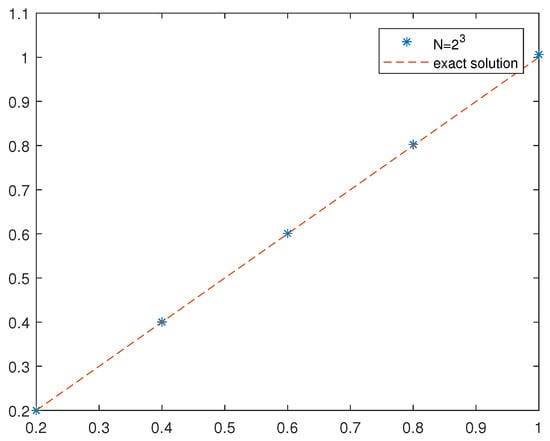
By applying the numerical method for $N=2^4,2^5,2^6,2^7$, and $2^8$, the obtained results at $t=0.4$ are shown in Table 3. As λ was not equal to μ, we first applied the Richardson $h^{2+\lambda }$ extrapolation, and then adopted the Richardson $h^{2+\mu }$ extrapolation. By comparing $E_h,E_{1,i}$ and $E_{2,i}$, these results verify the theoretical results, and we can see that the extrapolation improved the accuracy dramatically. When N = 8, 16, 32, 64, 128, the CPU time(s) are 1.43, 2.41, 3.99, 17.46, and 21.36 s, respectively. The exact solution and the approximation when N=8 are plotted in Figure 1.

Table 3. Numerical results at $t=0.4$ of Example 3.

N	${\mathit{E}}_{\mathit{h}}$	Rate	${\mathit{E}}_{1,\mathit{i}}$	${\mathit{E}}_{2,\mathit{i}}$	Posteriori Errors
$2^4$	$9.36\times {10}^{-5}$	—	—	—	—
$2^5$	$3.23\times {10}^{-5}$	$2^{1.53}$	$4.12\times {10}^{-6}$	—	$2.82\times {10}^{-5}$
$2^6$	$1.06\times {10}^{-5}$	$2^{1.61}$	$6.00\times {10}^{-7}$	$8.89\times {10}^{-7}$	$9.99\times {10}^{-6}$
$2^7$	$3.41\times {10}^{-6}$	$2^{1.63}$	$1.17\times {10}^{-7}$	$8.70\times {10}^{-8}$	$3.30\times {10}^{-6}$
$2^8$	$1.10\times {10}^{-6}$	$2^{1.65}$	$2.31\times {10}^{-8}$	$1.68\times {10}^{-8}$	$1.07\times {10}^{-6}$

Figure 1. The absolute errors and the approximations when N = 2${}^3$.

8. Conclusions

In this paper, by using the improved trapezoidal quadrature formula and linear interpolation, we obtained the approximate equation for non-linear Volterra integral equations with vanishing delay and weak singular kernels. The approximate solutions were obtained by an iterative algorithm, which possessed a high accuracy order $O(h^{2+\gamma })$. Additionally, we analyzed the existence and uniqueness of both the exact and approximate solutions. The significance of this work was that it demonstrated the efficiency and reliability of the Richardson extrapolation. The computational findings were compared with the exact solution: we found that our methods possess high accuracy and low computational complexity, and the results showed good agreement with the theoretical analysis. For future work, we can apply this method for solving two-dimensional delay integral equations.

References

- Avaji, M.; Hafshejani, J.; Dehcheshmeh, S.; Ghahfarokhi, D. Solution of delay Volterra integral equations using the Variational iteration method. J. Appl. Sci. 2012, 12, 196–200. [Google Scholar] [CrossRef]
- Williams, L.R.; Leggett, R.W. Nonzero Solutions of Nonlinear Integral Equations Modeling Infectious Disease. Siam J. Math. Anal. 1982, 13, 121. [Google Scholar] [CrossRef]
- Volterra, V. On some questions of the inversion of definite integrals. (Sopra alcune questioni di inversione di integrali definiti). Ann. Mat. Pura Appl. 1897, 25, 139–178. [Google Scholar] [CrossRef]
- Yang, K.; Zhang, R. Analysis of continuous collocation solutions for a kind of Volterra functional integral equations with proportional delay. J. Comput. Appl. Math. 2011, 236, 743–752. [Google Scholar] [CrossRef]
- Xie, H.; Zhang, R.; Brunner, H. Collocation methods for general Volterra functional integral equations with vanishing delays. SIAM J. Sci. Comput. 2011, 33, 3303–3332. [Google Scholar] [CrossRef]
- Ming, W.; Huang, C.; Zhao, L. Optimal superconvergence results for Volterra functional integral equations with proportional vanishing delays. Appl. Math. Comput. 2018, 320, 292–301. [Google Scholar] [CrossRef]
- Mokhtary, P.; Moghaddam, B.P.; Lopes, A.M.; Machado, J.A.T. A computational approach for the non-smooth solution of non-linear weakly singular Volterra integral equation with proportional delay. Numer. Algorithms 2019, 83, 987–1006. [Google Scholar] [CrossRef]
- Gu, Z.; Chen, Y. Chebyshev spectral-collocation method for a class of weakly singular Volterra integral equations with proportional delay. J. Numer. Math. 2014, 22, 311–342. [Google Scholar] [CrossRef]
- Zhang, R.; Zhu, B.; Xie, H. Spectral methods for weakly singular Volterra integral equations with pantograph delays. Front. Math. China 2014, 8, 281–299. [Google Scholar] [CrossRef]
- Brunner, H. Collocation Methods for Volterra Integral and Related Functional Differential Equations; Cambridge University Press: Cambridge, UK, 2004. [Google Scholar]
- Zhang, G.; Song, M. Impulsive continuous Runge—Kutta methods for impulsive delay differential equations. Appl. Math. Comput. 2019, 341, 160–173. [Google Scholar] [CrossRef]
- Shu, H.; Xu, W.; Wang, X.; Wu, J. Complex dynamics in a delay differential equation with two delays in tick growth with diapause. J. Differ. Equ. 2020, 269, 10937–10963. [Google Scholar] [CrossRef]
- Fang, J.; Zhan, R. High order explicit exponential Runge—Kutta methods for semilinear delay differential equations. J. Comput. Appl. Math. 2021, 388, 113279. [Google Scholar] [CrossRef]
- Song, H.; Xiao, Y.; Chen, M. Collocation methods for third-kind Volterra integral equations with proportional delays. Appl. Math. Comput. 2021, 388, 125509. [Google Scholar]
- Brunner, H. The numerical solution of weakly singular Volterra functional integro-differential equations with variable delays. Commun. Pure Appl. Anal. 2006, 5, 261–276. [Google Scholar] [CrossRef]
- Huang, C. Stability of linear multistep methods for delay integro-differential equations. Comput. Math. Appl. 2008, 55, 2830–2838. [Google Scholar] [CrossRef]
- Sheng, C.; Wang, Z.; Guo, B. An hp-spectral collocation method for nonlinear Volterra functional integro-differential equations with delays. Appl. Numer. Math. 2016, 105, 1–24. [Google Scholar] [CrossRef]
- Abdi, A.; Berrut, J.P.; Hosseini, S.A. The Linear Barycentric Rational Method for a Class of Delay Volterra Integro-Differential Equations. J. Sci. Comput. 2018, 75, 1757–1775. [Google Scholar] [CrossRef]
- Yaghoobi, S.; Moghaddam, B.P.; Ivaz, K. An efficient cubic spline approximation for variable-order fractional differential equations with time delay. Nonlinear Dyn. 2017, 87, 815–826. [Google Scholar] [CrossRef]
- Rahimkhani, P.; Ordokhani, Y.; Babolian, E. A new operational matrix based on Bernoulli wavelets for solving fractional delay differential equations. Numer. Algorithms 2017, 74, 223–245. [Google Scholar] [CrossRef]
- Rakhshan, S.A.; Effati, S. A generalized Legendre—Gauss collocation method for solving nonlinear fractional differential equations with time varying delays. Appl. Numer. Math. 2019, 146, 342–360. [Google Scholar] [CrossRef]
- Zuniga-Aguilar, C.J.; Gomez-Aguilar, J.F.; Escobar-Jimenez, R.F.; Romero-Ugalde, H.M. A novel method to solve variable-order fractional delay differential equations based in lagrange interpolations. Chaos Solitons Fractals 2019, 126, 266–282. [Google Scholar] [CrossRef]
- Xu, X.; Huang, Q. Superconvergence of discontinuous Galerkin methods for nonlinear delay differential equations with vanishing delay. J. Comput. Appl. Math. 2019, 348, 314–327. [Google Scholar] [CrossRef]
- Bellour, A.; Bousselsal, M. A Taylor collocation method for solving delay integral equations. Numer. Algorithms 2014, 65, 843–857. [Google Scholar] [CrossRef]
- Darania, P.; Sotoudehmaram, F. Numerical analysis of a high order method for nonlinear delay integral equations. J. Comput. Appl. Math. 2020, 374, 112738. [Google Scholar] [CrossRef]
- Khasi, M.; Ghoreishi, F.; Hadizadeh, M. Numerical analysis of a high order method for state-dependent delay integral equations. Numer. Algorithms 2014, 66, 177–201. [Google Scholar] [CrossRef]
- Bica, A.M.; Popescu, C. Numerical solutions of the nonlinear fuzzy Hammerstein-Volterra delay integral equations. Inf. Sci. 2013, 223, 236–255. [Google Scholar] [CrossRef]
- Mosleh, M.; Otadi, M. Least squares approximation method for the solution of Hammerstein-Volterra delay integral equations. Appl. Math. Comput. 2015, 258, 105–110. [Google Scholar] [CrossRef]
- Zhang, X. A new strategy for the numerical solution of nonlinear Volterra integral equations with vanishing delays. Appl. Math. Comput. 2020, 365, 124608. [Google Scholar]
- Lima, P.; Diogo, T. Numerical solution of a nonuniquely solvable Volterra integral equation using extrapolation. J. Comput. Appl. Math. 2002, 140, 537–557. [Google Scholar] [CrossRef]
- Sidi, A. Practical Extrapolation Methods; Cambridge University Press: Cambridge, UK, 2003. [Google Scholar]
- Tao, L.; Jin, H. High Precision Algorithm for Integral Equations; China Science Press: Beijing, China, 2013. [Google Scholar]
- Tao, L.; Yong, H. Extrapolation method for solving weakly singular nonlinear Volterra integral equations of the second kind. J. Math. Anal. Appl. 2006, 324, 225–237. [Google Scholar] [CrossRef]
- Navot, J. A Further Extension of the Euler-Maclaurin Summation Formula. J. Math. Phys. 1962, 41, 155–163. [Google Scholar] [CrossRef]
- Tao, L.; Yong, H. A generalization of Gronwall inequality and its application to weakly singular Volterra integral equation of the second kind. J. Math. Anal. Appl. 2003, 282, 56–62. [Google Scholar] [CrossRef]
- Qin, Y. Integral and Discrete Inequalities and Their Applications; Springer International Publishing: Berlin/Heidelberg, Germany, 2016. [Google Scholar]
Publisher’s Note: MDPI stays neutral with regard to jurisdictional claims in published maps and institutional affiliations. |
© 2021 by the authors. Licensee MDPI, Basel, Switzerland. This article is an open access article distributed under the terms and conditions of the Creative Commons Attribution (CC BY) license (https://creativecommons.org/licenses/by/4.0/).