On the Connection between the GEP Performances and the Time Series Properties

Abstract

Artificial intelligence (AI) methods are interesting alternatives to classical approaches for modeling financial time series since they relax the assumptions imposed on the data generating process by the parametric models and do not impose any constraint on the model’s functional form. Even if many studies employed these techniques for modeling financial time series, the connection of the models’ performances with the statistical characteristics of the data series has not yet been investigated. Therefore, this research aims to study the performances of Gene Expression Programming (GEP) for modeling monthly and weekly financial series that present trend and/or seasonality and after the removal of each component. It is shown that series normality and homoskedasticity do not influence the models’ quality. The trend removal increases the models’ performance, whereas the seasonality elimination results in diminishing the goodness of fit. Comparisons with ARIMA models built are also provided.

1. Introduction

Financial time series analysis and forecasting have been interesting research fields for decades. Time series analysis may explain the law governing the data generating process, while good models may provide accurate predictions of its future behavior, supporting the decisions for profitable trading strategies [1,2].

From the apparition of the Box–Jenkins methodology [3] for times series analysis and forecast, ARIMA and SARIMA models have been extensively used to forecast financial time series [4,5]. In 1989, Hamilton [6] introduced the Markov Switching Model, which became one of the most popular models used for the nonlinear series, involving multiple equations that characterize the series behavior in different regimes [7]. The switching mechanism has also been incorporated in conditional variance models, such as stochastic volatility models [8] or GARCH [9]. Recent studies suggest that GARCH [10,11] can be a promising alternative to the traditional SARIMA method in forecasting problems, especially for nonlinear data. Still, it was shown that it is difficult to find such models with very high accuracy for long series with high variability.

The efficient market hypotheses, which assert that the market is efficient, attracted many criticisms from behavioral economists or psychologists. Introduced by Lo [12], for the reconciliation of the economic theories based on the efficient market hypothesis with behavioral economics, the adaptive market hypotheses apply the principles of evolution (competition, adaptation, and natural selection) [13]. The present study is in line with this theory.

Last period, artificial intelligence methods were extensively used for modeling financial series [14,15] because the traditional statistical methods cannot capture high nonlinearity and discontinuities. It seems that the evolutionary algorithms have the learning capacity of capturing the nonlinear future (which is dominant in financial series) [16,17], having the advantage to not rely on a specific form of the fitting model. Approaches like support vector regression [15,18,19], neural networks [14,20], or hybrid algorithms provided [13,21] valuable solutions to modeling economic and financial problems.

Part of the family of evolutionary techniques, the genetic programming paradigm, is defined as a generalization of Holland’s genetic algorithms. Starting from Koza’s seminal work [22], many algorithms have been developed as alternatives to genetic programming. One of them is Gene Expression Programming (GEP) [23], which was successfully used for modeling economics problems. For example, Huang et al. [24] used the GEP to generate trading signals for stocks, Chen et al. [16,25] utilized the Sortino ratio for fund selection, followed by the application of GEP for evolving dynamic trading strategies for them. Modeling economics problems, forecasting mutual funds, and financial indices’ evolution have also been conducted by other scientists [13,15,25,26,27,28,29,30,31,32,33].

Despite the significant number of articles in this field, only one investigated the relationship between the statistical properties of some financial series and the AI models’ goodness of fit. Still, it refers to the generalized regression neural networks [14]. Therefore, this study will fill a gap in this field. We analyze the statistical properties of different financial time series and investigate the connection between these properties and the GEP models’ goodness of fit. Comparisons of these models with the classical ARIMA are also provided, showing better performances of the GEP models. The research is important for selecting the best model from a diversity of options.

2. Materials and Methods

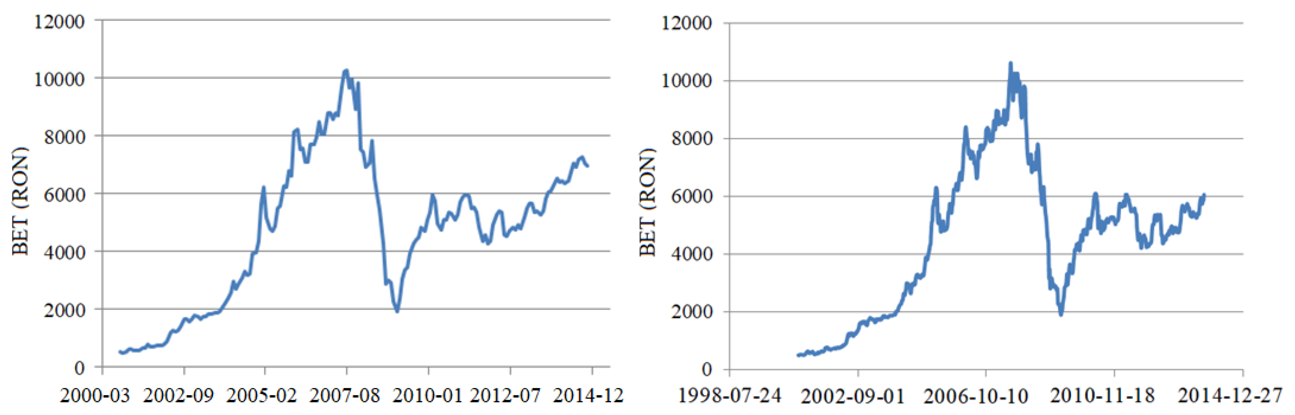
2.1. Studied Data and Statistical Tests

The data studied here consist of the BET index closing values, monthly series registered during October 2000–September 2014, and weekly series recorded in the period 1 October 2000–29 September 2014, downloaded from the website of the Bucharest Stock Exchange (BSE) [34]. Both series are complete, without gaps. The BET monthly and weekly series are represented in Figure 1.

BET, the first index developed by BSE, is a free-float weighted capitalization index with ten constituents being the reference index for BSE. BET reflects the performance of the most traded Romanian companies, listed at BVB, meeting the highest standards in the fields of investor relations and corporate governance. Constituents’ weights are capped quarterly to ensure that they fulfill the standards for portfolio diversification [35].

Since the series presents high variability, we took the logarithms of their values. The resulted monthly and weekly data series are denoted by S_m and S_w, respectively.

Statistical tests have been performed at the significance level of 5% for S_m, S_w, and their subseries determined after the change point detection. The null and alternative hypotheses (denoted by H₀ and H₁, respectively) of these tests are presented in

Table 1. Tests performed for data analysis.

No.	Type of Test	Null and Alternative Hypotheses	Tests Performed
I.	Normality	H0: The series is Gaussian H1: The series is not Gaussian	Robust Jarque-Bera [36], Anderson-Darling, and Shapiro-Wilk tests [37]
II.	Homoskedasticity	H0: The series is homoskedastic H1: The series is heteroskedastic	Levene test [38]
III.	Randomness	H0: The series comes from a random process H1: The series does not come from a random process	Runs test [39,40] Autocorrelation function [41]
IV.	Trend existence	H0: The series does not have a monotonic trend H1: The series has a monotonic trend	Mann-Kendall test [42]
V.	Unit root tests	H0: The series has a unit root H1: The series is stationary	Augmented Dickey-Fuller test (ADF) [43], Phillips-Perron test(PP) [44]
VI.	Stationarity	H0: The series is stationary (a) in level or (b) around a deterministic trend H1: The series is not stationary (a) in level or (b) around a deterministic trend	KPSS test [45]
VII.	Breakpoint	H0: The series has no breakpoint H1: The series has at least a breakpoint	Pettitt test [46], CUSUM [47], mDP [48]

, together with the references. Since the statistical tests are well-known, they are not discussed in detail here. For a deeper insight into them, readers may refer to [36,37,38,39,40,41,42,43,44,45,46,47,48,49].

2.2. Methods

For modeling purposes, gene expression programming (GEP) was used.

GEP is an algorithm for implementing symbolic regression, that does not request the advanced specification of the form of the function be determined.

In GEP, an individual is a solution to the problem, with all the individuals (e.g., the problem’s solutions) forming a population. GEP individuals are represented by hierarchical mathematical expressions, encoded as multi-genic linear chromosomes of a fixed length, which are linear strings of functional symbols (+, −, ∗, /, and functions—exponential, trigonometric, logarithmic, etc.), variables (containing the lagged values of the time series), and constants [13].

A gene is composed of a head (that may contain any symbol) and a tail (containing only constants and variables). The user must set the number of genes and the set of symbols before running the algorithm.

The word generation describes an iteration of the algorithm, pointing out the evolutionary aspect of the search process. The initial generation of individuals is randomly selected.

An iteration of the algorithm consists of modifying the individuals and choosing them based on their quality. The individuals’ modifications are realized by applying genetic operators: crossover, mutation, and transposition. Crossover combines the features of two or more parent individuals into one or more children. The mutation alters an individual, modifying some of its features. The gene transposition randomly chooses one of the chromosome’s genes and moves it in the place of another gene.

The fitness function evaluates the solution quality.

GEP was used with good results for solving symbolic regression problems and time series forecasting. In the context of time series modeling, a candidate solution is a mathematical expression formed by functions, variables, and constants, and as a consequence, it is represented as a parse tree of the mathematical expression [20,23].

If (x_t) (t = 1,…,n) represent the values of the data series and ${\left(\widehat{x_t}\right)}_{t=1, \dots ,n}$ are those computed by the algorithm, GEP aims to determine a function f that estimates the registered value at a moment t (t < n), as best as possible, such that $\widehat{x_t}=f\left(x_{t-1}, \dots ,x_{t-w}\right),$ where w is a window size, and $x_{t-1}, \dots ,x_{t-w}, 0\le t-w\le n$ are the previous w values.

The analytical form of the function is not specified, being the result of the evolution of the mathematical expressions in the algorithm.

The basic structure of the gene expression algorithm is [23]:

(1)

Create chromosomes of the initial population;

(2)

Express chromosomes and evaluate their fitness;

• If the stopping criterion is satisfied, designate results and stop;
• If stopping criterion is not satisfied, go to the next step;

(3)

Select chromosomes and keep the fittest for the next generation;

(4)

Perform genetic modifications via genetic operators and gene recombination;

(5)

Select next-generation individuals;

(6)

Go to (2).

The termination criterion is the number of generations.

The accuracy of a model for a series of n observations is measured by the correlation between the actual and predicted values, the root mean squared error (RMSE), the mean squared error (MSE), the mean absolute error (MAE), and the mean absolute percentage error (MAPE) [13,14].

The settings for GEP parameters utilized in the present study (typical in the literature) are: the population size—50, the number of genes per chromosome—4, the gene head length—8, the maximum generations—2000, and the number of generations without improvement—1000. The settings of the evolution rate were: mutation rate—0.044, inversion rate—0.1, transposition rates—0.1, recombination rates: one point—0.3, two-point—0.3, gene rate—0.1. Other settings, recommended by the literature [13,16,22,23] and used for running the algorithm are:

• The window size, w, was considered between 1 and 12. In the following, we report only the overall best result experiments;
• The mutation rate of random constants: 0.01;
• Maximum number of iterations: 1000;
• Functions used in expressions: addition, subtraction, multiplication, division, square root;
• Linking function: addition.
• The fitness function is the mean squared error (MSE):

$$MSE=\sqrt{\frac{1}{n}{\displaystyle \sum _{i=1}^n{\left(x_i-{\widehat{x}}_i\right)}^2}}$$

(1)

where $x_i$ is the actual value and ${\widehat{x}}_i$ is the computed value.

The best solution is the one with the smallest fitness.

The studied series was divided into two parts, the first one for training (70% of data) and the rest for the test (30% of data). The model was built using the training data (the algorithm learns the data on this set) and was validated on the test set.

The GEP was chosen for modeling purposes, since it is computationally faster than the methods based on neural networks and support vector regression, and generally gives better results in comparison to them.

For details about GEP and its applications, readers may refer to [20,23,49].

ARIMA models have been built as benchmark models for the series and their subseries determined by the change points.

A linear process ($X_t$)($t\in Z$) is called autoregressive of p order—AR(p)—if

$$X_t={\displaystyle \sum }_{i=1}^p{\phi }_i{X}_{t-i}+{\epsilon }_t,{\phi }_p\ne 0, t\in Z$$

(2)

where $\left({\epsilon }_t, t\in Z\right)$ is a white noise with the variance σ².

Defining

$$\mathsf{\Phi }\left(z\right)=1-{\phi }_{1}z-\dots -{\phi }_p{z}^p,$$

(3)

the Equation (2) becomes

$$\left(1-{\phi }_{1}B-\dots -{\phi }_p{B}^p\right)X_t={\epsilon }_t$$

(4)

or

$$\mathsf{\Phi }\left(B\right)X_t={\epsilon }_t$$

(5)

where (${\epsilon }_t, t\in Z$) is a white noise with the variance ${\mathsf{\sigma }}^2,$ B is the backshift operator (defined by $B(X_t)=X_{t-1}$) and $B^k\left(X_t\right)=X_{t-k}.$

A linear process ($X_t$) ($t\in Z$) is called moving average of q order—MA(q)—if

$$X_t={\epsilon }_t-{\displaystyle \sum }_{j=1}^q{\theta }_j{\epsilon }_{t-j}+{\epsilon }_t, {\theta }_q\ne 0, t\in Z$$

(6)

where $\left({\epsilon }_t, t\in Z\right)$ is a white noise with the variance σ².

Defining

$$\mathsf{\Theta }\left(z\right)=1-{\theta }_{1}z-\dots -{\theta }_q{z}^q,$$

(7)

the relation (6) becomes

$$\mathsf{\Theta }\left(B\right){\epsilon }_t=X_t$$

(8)

A linear process ($X_t$) ($t\in Z$) is called an autoregressive moving average of p, q orders ARMA(p, q) if

$$\mathsf{\Phi }\left(B\right)X_t=\mathrm{c}+\mathsf{\Theta }\left(B\right){\epsilon }_t$$

where $\left({\epsilon }_t, t\in Z\right)$ is a white noise with the variance σ². The constant c is called drift.

An autoregressive integrated moving average process ARIMA (p, d, q) is defined by the equation

$$\mathsf{\Phi }\left(B\right){\mathsf{\Delta }}^d{X}_t=\mathsf{\Theta }\left(B\right){\epsilon }_t$$

(9)

where ${\mathsf{\Delta }}^d{X}_t=$(1 − B)^d$X_t$ (d > 0) the absolute values of Φ şi Θ are greater than 1 and $\left({\epsilon }_t, t\in Z\right)$ is a centered white noise.

To select the best ARIMA model, the Akaike (AIC) criterion was used. The lower the AIC is, the better the model is.

For a deeper insight into ARIMA models, the reader may refer to [41].

Statistical tests and modeling were performed using the R and DTREG software.

3. Results and Discussion

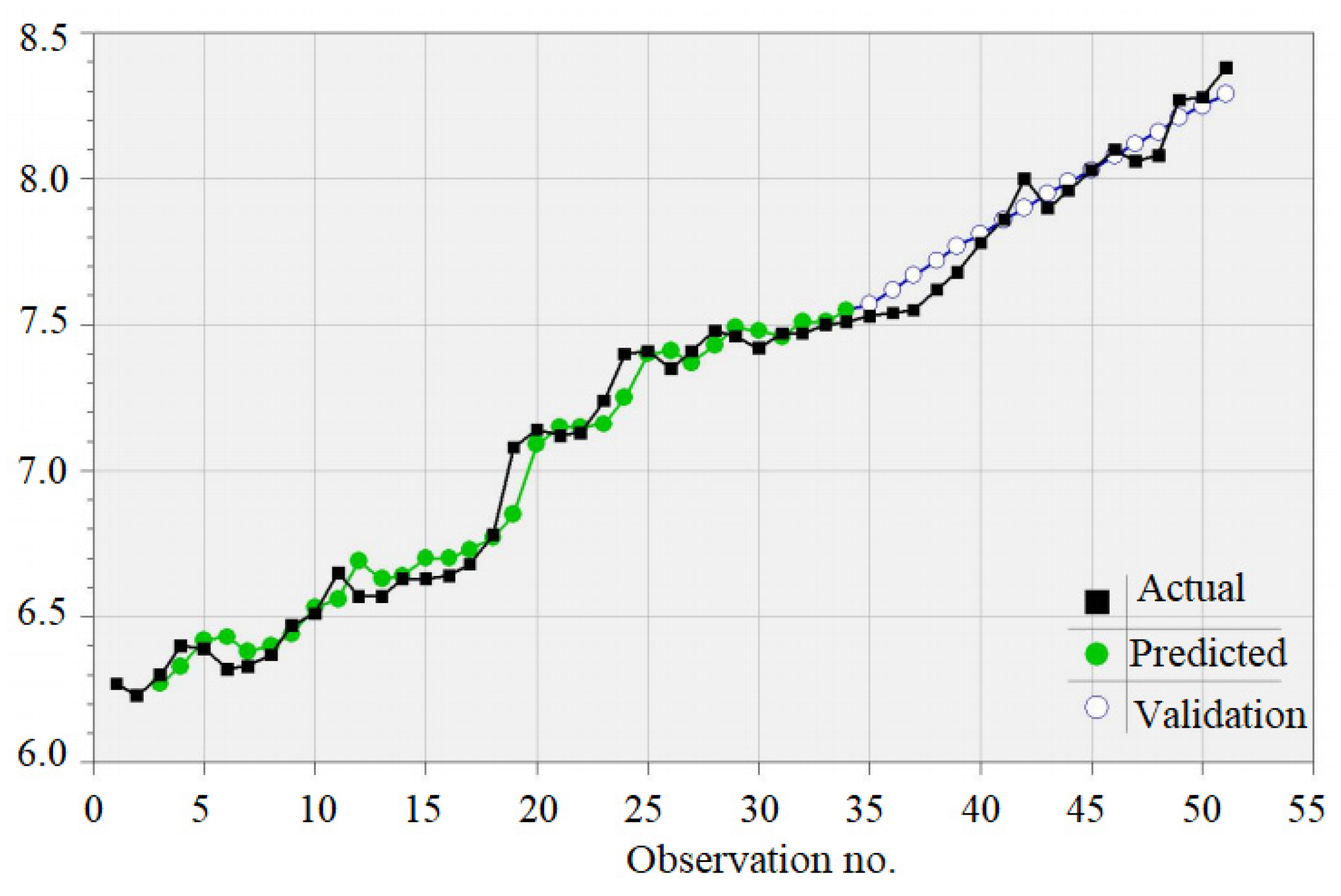
3.1. Results of Statistical Analysis and the GEP Models for the Monthly Series

The results of the statistical analysis of the lnBET monthly series are the following. The normality and homoskedasticity hypotheses were rejected. After the application of the runs test, the null hypothesis was rejected. The analysis of the correlogram confirms the existence of the data autocorrelation. After performing the Mann–Kendall test, the alternative hypothesis of the existence of a monotonic trend could not be rejected. Both ADF and PP tests did not support the rejection of the existence of a unit root, while the KPSS rejected the hypothesis of series’ stationarity in level or around a deterministic trend. After taking the first-order difference, the ADF and PP tests rejected the existence of the unit root, while the KPSS test did not reject the hypothesis of the stationarity in level and around a deterministic trend.

The Pettitt test provides December 2004 (the 51st value of the series) as a breakpoint, while the mDP algorithm and CUSUM detected December 2004, November 2007 (86th value of the series), and March 2009 (102nd value of the series) as change points.

The same statistical tests have been performed for each subseries, detected after the segmentation. Here are the notations used in the rest of the paper for the above monthly series: S_m is lnBET, S1_m—the series containing the first 51 values of S series (October 2000–December 2004), S2_m—the series containing the values from the 52nd one to the 86th one (January 2005–November 2007), S3_m—the series containing 16 values recorded from December 2007 to March 2009, S4_m—the series registered in the period April 2009 –September 2014 (the last 66 values), U1_m—the series recorded between January 2005 and September 2014.

For each monthly series and subseries, the Mann–Kendall test [42] was used for testing the hypothesis that the series does not have a monotonic trend (H₀) against the existence of such a trend (H₁).

The results of all the tests are presented in

Table 2. Results of statistical tests on the monthly series.

	Type of Test	Series
		S_m	S1_m	S2_m	S3_m	S4_m	U1_m
I.	Normality	yes	yes	no	no	no	yes
II.	Homoskedasticity	yes	no	yes	no	no	yes
III.	Randomness	yes	yes	yes	yes	yes	yes
IV.	Trend existence	yes	yes	yes	yes	yes	no
V.	Unit root	no	no	no	no	no	no
VI.	a. Level stationarity	yes	yes	yes	yes	yes	yes
	b. Trend stationarity	yes	yes	yes	no	yes	yes

, where yes means that H₀ is rejected, and no means that H₀ cannot be rejected.

For building GEP models for the monthly series, the window size, w, was selected between 1 and 12, considering the possible existence of a seasonal component. The performances of the best models are presented in

Table 3. Performances of the best models built for the monthly series with lag 1 variables as regressors.

Series	Training					Test
	S_m	S1_m	S2_m	S3_m	S4_m	S_m	S1_m	S2_m	S3_m	S4_m
Correlation actual- predicted values	0.965	0.893	0.850	0.785	0.743	0.617	0.980	0.570	0.577	0.960
RMSE	0.213	0.213	0.102	0.234	0.101	0.405	0.141	0.070	0.130	0.096
MSE	0.053	0.045	0.010	0.016	0.010	0.164	0.020	0.004	0.016	0.009
MAE	0.091	0.087	0.072	0.118	0.057	0.355	0.114	0.055	0.118	0.086
MAPE	1.205	1.323	0.830	1.529	0.690	4.129	1.421	0.608	1.529	0.979
Removed trend	none	none	none	none	none	none	none	none	none	none

,

Table 4. The goodness of fit indicators for the best models built for the monthly series with lag 1 and lag 12 variables as regressors.

Series	Training				Test
	S_m	S1_m	S2_m	S4_m	S_m	S1_m	S2_m	S4_m
Correlation actual-predicted values	0.965	0.895	−0.292	0.743	0.558	0.980	0.200	−0.874
RMSE	0.228	0.212	0.275	0.096	0.147	0.226	0.097	0.239
MSE	0.052	0.044	0.075	0.009	0.021	0.051	0.009	0.057
MAE	0.091	0.087	0.193	0.056	0.123	0.184	0.074	0.215
MAPE	1.203	1.320	2.239	0.669	1.419	2.274	2.811	2.451

,

Table 5. The goodness of fit indicators for the best models built for U1_m.

Indicators	Regressors: Lag 1 and Lag 12		Regressors: Lag 1
	Training Test		Training Test
Correlation actual-predicted values	0.958	0.515	0.956	−0.933
RMSE	0.101	0.136	0.104	0.183
MSE	0.010	0.018	0.010	0.033
MAE	0.073	0.114	0.074	0.151
MAPE	0.868	1.312	0.879	1.729

,

Table 6. The equations of the trend for the monthly series and subseries.

	Trend Equation	Variance Explained by the Trend
S_m	Yt = 7.2878 + 0.0112t	47.938%
S1_m	Yt = 6.1794 + 0.0422t	97.307%
U1_m	Yt = 8.5511 + 0.3236$e^{-0.0264t}$	7.392%
S2_m	Yt = 8.5607 + 0.0202t	84.604%
S3_m	Yt = 10.2396 − 1.0992$e^{-0.0604t}$	92.758%
S4_m	Yt = 8.3897 + 0.03742$e^{-0.0388t}$	54.772%

Note. Y_t denotes the trend and t is the time.

and

Table 7. Performances of the best models built for the detrended monthly series with lag 1 variable as regressors.

Indicators/Series	Training					Test
	S_md	S1_md	S2_md	S3_md	S4_md	S_md	S1_md	S2_md	S3_md	S4_md
Correlation actual- predicted values	0.988	0.988	0.927	0.810	0.576	0.975	0.980	0.567	0.699	0.942
RMSE	0.130	0.070	0.071	0.124	0.084	0.485	0.062	0.073	0.150	0.034
MSE	0.017	0.005	0.005	0.015	0.007	0.236	0.003	0.005	0.022	0.001
MAE	0.078	0.054	0.058	0.097	0.053	0.426	0.050	0.056	0.115	0.025
MAPE	1.006	0.791	0.664	1.126	0.633	4.956	0.630	0.625	1.482	0.290
Removed trend	linear	linear	linear	exp	exp	linear	linear	linear	exp	exp

for the training and test sets.

Table 3, Table 4 and Table 5 contain the results of the modeling of the monthly series without the trend removal, when the regressors were lag 1, and lag 1 and lag 12 variables, respectively. Since S3_m is too short, the model with lag 1 and lag 12 variables could not be built.

When analyzing the goodness of fit indicators for the series S_m and S1_m, one can see that the models’ performances on the training sets are not significantly different when lag 1 and lag 12 variables, or only lag 1 variables are considered.

The two-sided Diebold–Mariano test [50] was also used to cross-validate these findings. The null hypothesis was (H₀) Both models have the same accuracy, and the alternative was (H₁) The models do not have the same accuracy.

The p-values were 0.341 (0.532), when comparing the models for S_m (S1_m) on the training set. Therefore, the null hypothesis could not be rejected.

The model for S_m is better on the test set when using both regressors than when using only the first one (lag 1 variable), in terms of all indicators but the correlation between the actual and predicted values. The result of the Diebold–Mariano test confirms this assertion. This time the null hypothesis was the same as previously, while the alternative one was (H_1′) The model obtained using both regressors is better than the models obtained utilizing lag 1 regressor.

Comparing the goodness of fit indicator, the results for the S1_m model are better when considering only the lag 1 regressor. Still, the two-sided Diebolo–Mariano test does not reject the null hypothesis.

The models obtained for S2_m and S4_m are better when using only the lag 1 variable, than when using lag 1 and lag 12 because a negative correlation between the actual and predicted values is noticed in the second case.

From the point of view of the correlation between actual and predicted values, GEP models with lag 1 regressors perform satisfactorily on both training and test sets, the best results being obtained for S1_m and S4_m. Since the models with lag 1 variables as regressors are better, in terms of correlation between the actual and predicted values, we kept these models for further comparisons.

For U1_m (Table 5), the quality of the model obtained with lag 1 variable is worse than that obtained with lag 1 and lag 12 as regressors on the test set (see the negative value of the correlation between actual and predicted values), but on the training one, the results are not significantly different (through applying the Diebold–Mariano two-sided test).

GEP models have been built for the detrended series and subseries, with the same variables as regressors. The models with significant coefficients and the highest variance of the series explained by the model (among the linear, exponential, polynomial of second and third degrees, and logarithmic) have been chosen to express the trend. The best trends were found to be linear or exponential, as presented in Table 6.

For S1_m, S3_m, and S2_m, the variance of the data series explained by the models is very high.

The following notations are adopted for the monthly detrended series and subseries: S_md, S1_md, S2_md, S3_md, S4_md, and U1_md, respectively.

Table 7,

Table 8. Performances of the best models built for the detrended monthly series and subseries with lag 1 and lag 12 variables as regressors.

Indicators/Series	Training				Test
	S_md	S1_md	S2_ md	S4_md	S_md	S1_md	S2_md	S4_md
Correlation actual-predicted values	0.989	0.991	0.928	0.989	0.448	0.839	0.444	0.448
RMSE	0.129	0.061	0.075	0.121	0.656	0.295	0.108	0.656
MSE	0.016	0.003	0.005	0.016	0.431	0.087	0.011	0.431
MAE	0.078	0.048	0.059	0.078	0.587	0.239	0.088	0.587
MAPE	1.009	0.711	0.681	1.009	6.828	3.023	0.977	6.828
Removed trend	linear	linear	linear	linear	linear	linear	linear	linear

and

Table 9. Performances of the best models built for U1_md.

Indicators	Regressors: Lag 1 and Lag 12		Regressors: Lag 1
	Training	Test	Training	Test
Correlation actual-predicted values	0.958	0.168	0.954	−0.916
RMSE	0.102	0.171	0.106	0.180
MSE	0.010	0.029	0.011	0.032
MAE	0.077	0.152	0.077	0.148
MAPE	0.902	1.754	0.904	1.694
Removed trend	linear	linear	exp	exp

contain the modeling results after the trend removal.

Table 7 shows that the trend removal improved the models’ performances (most significantly for S1_m and S4_m) on both training and test series, when the regressors were the lag 1 variables. Indeed, the MAPEs values diminished after the trend removal for all but the S_m series on the test set.

For example, Figure 2 presents the chart of S1_md (corresponding to the data from Table 7, columns 3 and 8). The equation of the detected linear trend in this model is:

Y_t = 6.179 + 0.042t

(10)

where t = 1,…,51 is the number of the month, and Y_t is the trend. The standard errors of the coefficients are respectively 0.0235 and 0.0142.

The equation of the GEP model is:

$$y_t=0.151y_{t-1}^2+0.7745y_{t-1}$$

(11)

The standard errors of the coefficients are respectively 0.0121 and 0.0415. All the model’s coefficients are significant, at a significance level of 0.05.

From Table 8, one remarks that the algorithm learns the input data well for the monthly series and its subseries, after the trend elimination. It better performs, in terms of correlation between the actual and predicted values on the test sets S2_md and S4_md.

A significantly diminished MAPE was computed for the S2_md test set. When the regressors are lag 1 and lag 12 variables, a notable improvement of the models is noticed only on the training set. The algorithm learns data well, but it cannot use what it learned on the test sets. Overall, the models’ performances are comparable or better with one regressor (Table 7) than with two regressors (Table 8).

The best models for U1_md have been obtained for two regressors (columns 2 and 3 from Table 9). The models for U1_md are better than those for U1, in terms of RMSE, MSE, MAE, and MAPE. Comparing the results from Table 5 and Table 9, one may remark that the trend removal contributed to improving the models’ quality when using lag 1 variables as regressors. Still, the model is not satisfactory, in terms of the correlation between actual and predicted values on the test series.

The next stage of this analysis was building the deseasonalized series (and subseries) and the corresponding GEP models. For this aim, the classical decomposition method was employed. The equation is:

$$y_t=Y_t+S_t+{\epsilon }_t$$

(12)

where $y_t$ is the series to be decomposed, $Y_t$ is the trend, $S_t$ is the seasonality index, and ${\epsilon }_t$, the random variable.

The difference $y_t-S_t$ is by definition the deseasonalized series.

In the following, the deseasonalized monthly series S is denoted by S_ms.

Analogous notations are used for the monthly subseries.

The performances of the best models are presented in

Table 10. Performances of the best models built for the deseasonalized monthly series its subseries with lag 1 variables as regressors.

Indicators/Series	Training				Test
	S_ms	S1_ms	S2_ms	S4_ms	S_ms	S1_ms	S2_ms	S4_ms
Correlation actual-predicted values	0.065	0.911	0.855	0.743	0.617	0.961	0.442	0.960
RMSE	0.231	0.198	0.096	0.101	0.405	0.212	0.105	0.096
MSE	0.053	0.039	0.009	0.010	0.164	0.044	0.011	0.009
MAE	0.091	0.080	0.055	0.057	0.355	0.187	0.083	0.086
MAPE	1.205	1.206	0.635	0.690	4.129	2.314	0.910	0.979
Removed trend	none	none	none	none	none	none	none	none

and

Table 11. Performances of the best models built for U1_ms.

Indicators/Series	Regressors: Lag 1 and Lag 12		Regressors: Lag 1
	Training	Test	Training	Test
Correlation actual-predicted values	0.958	0.420	0.956	−0.933
RMSE	0.102	0.112	0.104	0.184
MSE	0.010	0.031	0.011	0.034
MAE	0.152	0.097	0.075	0.151
MAPE	0.902	0.857	0.879	1.727
Removed trend	none	none	none	none

.

For S_ms, the correlation between the actual and predicted values on the training set is close to zero. On the test set, the same indicator is higher. Still, it remains lower than for the raw series or the detrended one. Generally, the models for the deseasonalized subseries are worse than those for the raw and detrended series.

For example, in Figure 3, one may see the modeling errors for S4_ms (Table 10, columns 5 and 9) which are very low compared to the data values (that are in the interval (7.916, 8.932)). The equation of the corresponding GEP model is

$$y_t=(2.7144406/\sqrt{y_{t-1}})+ y_{t-1}-0.9135744.$$

(13)

For U1_ms, the best model has been obtained for lag 1 and 12 as regressors.

To conclude, removing the seasonality did not improve the modeling quality.

3.2. Results of Statistical Analysis and the GEP Models for the Monthly Series

The change point determined by the Pettitt test for the weekly series is 215 (26 December 2004), and those found by mDP are 215 (26 December 2004), 365 (9 December 2007), 435 (26 April 2009). In what follows, the weekly series is denoted by S_w, and the subseries determined by the change points are denoted, respectively, by S1_w (containing the values 1–215), S2_w (containing the values 216–365), S3_w (containing the values 366–435), S4_w (containing the values 436–717), and U1_w (containing the values 216–717). The subseries and the fitted linear trend are presented in Figure 4.

Table 12. The equations of the trend for the weekly series and subseries.

	Trend Equation	Variance Explained by the Trend
S_w	Yt = 7.2800 + 0.0026t	47.650%
S1_w	Yt = 6.1372 + 0.0100t	97.412%
U1_w	Yt = 8.7731 − 0.0005 t	5.589%
S2_w	Yt = 8.5569 + 0.0047t	86.379%
S3_w	Yt = 11.3341 − 2.1602$e^{0.0081t}$	89.660%
S4_w	Yt = 8.4420 + 0.0117$e^{0.0137t}$	49.732%

contains the equations of the trend lines of the weekly series. The coefficients and the models are significant at a 0.05 significance level (based on the t-test and the F-test). The trend determined for the series and subseries is the best fit for the data series, selected from a set of deterministic models (linear, exponential, polynomial of the second and third-order, logarithmic, and power functions).

The results of the statistical tests on the weekly series are presented in

Table 13. Results of statistical tests on the weekly series.

	Type of Test	Series
		S_w	S1_w	S2_w	S3_w	S4_w	U1_w
I.	Normality	yes	yes	yes	yes	yes	yes
II.	Homoskedasticity	yes	yes	yes	yes	yes	yes
III.	Randomness	yes	yes	yes	yes	yes	yes
IV.	Trend existence	yes	yes	yes	yes	yes	yes
V.	Unit root	no	no	no	no	no	no
VI.	a. Level stationarity	yes	yes	yes	yes	yes	yes
	b. Trend stationarity	yes	yes	yes	yes	yes	yes

. For all tests except normality and homoskedasticity, they are similar to those for the monthly series. To summarize, the hypotheses that the series are Gaussian, homoskedastic, stationary (in trend and level), and are not random, have been rejected, while the unit root hypothesis could not be rejected. Therefore, the series differentiation has been performed for finding the best ARIMA model (presented in the next section).

A window size from one to five has been considered when selecting the best GEP models for the weekly series. Therefore, in the models, the regressors were the lagged variables from one to five. These lag values have been selected because the actual values could be influenced by the values from the same week (and taking into account that during Saturdays and Sundays, the stocks are not traded at BSE). The best GEP models for the weekly series are presented in

Table 14. Performances of the best models built for S_w and its subseries.

Series	Training						Test
	S_w	S1_w	S2_w	S3_w	S4_w	U1_w	S_w	S1_w	S2_w	S3_w	S4_w	U1_w
Correlation actual-predicted values	0.992	0.976	0.957	0.952	0.930	0.991	0.610	0.968	0.604	0.268	0.901	0.916
RMSE	0.111	0.102	0.053	0.101	0.052	0.048	0.226	0.080	0.055	0.216	0.042	0.063
MSE	0.012	0.010	0.003	0.010	0.003	0.002	0.051	0.006	0.003	0.047	0.002	0.004
MAE	0.034	0.032	0.030	0.055	0.027	0.032	0.197	0.066	0.045	0.149	0.031	0.055
MAPE	0.448	0.493	0.339	0.638	0.323	0.380	2.294	0.828	0.491	1.887	0.356	0.642
Regressors (lag)	1 & 5	1	1 & 5	1	1 & 5	1 $÷$ 5	1 & 5	1	1 & 5	1	1 & 5	1 $÷$ 5

.

The models for S1_w, S3_w, and S4_w are good on both training and test sets. The correlations between actual and predicted values on the training sets are high for the other subseries, but they are much lower for the test set (0.610 for S_w and 0.268 for S3_w). On the same test sets, MAPEs are 2.294 and 1.887, confirming that the algorithm does not apply what it learned on the test sets S_w and S3_w. Since the data series are not monthly or annual, the seasonal component does not appear.

The study results on the detrended series are presented in

Table 15. Performances of the best models built for the S_w and its subseries, after the trend removal. The detrended series are denoted by S_wd, S1_wd, S2_wd, S3_wd, S4_wd, and U1_wd.

Series	Training						Test
	S_wd	S1_wd	S2_wd	S3_wd	S4_wd	U1_wd	S_wd	S1_wd	S2_wd	S3_wd	S4_wd	U1_wd
Correlation actual-predicted values	0.998	0.997	0.982	0.981	0.944	0.989	0.556	0.976	0.600	0.213	0.938	0.836
RMSE	0.060	0.033	0.034	0.065	0.046	0.050	0.487	0.058	0.059	0.204	0.045	0.187
MSE	0.004	0.001	0.001	0.004	0.002	0.002	0.237	0.003	0.003	0.041	0.002	0.035
MAE	0.032	0.025	0.025	0.043	0.026	0.032	0.439	0.049	0.046	0.142	0.037	0.152
MAPE	0.405	0.367	0.285	0.505	0.307	0.380	5.101	0.620	0.507	1.803	0.423	1.740
Removed trend	lin.	lin.	lin.	exp	exp	lin	lin	lin.	lin.	exp	exp	lin
Regressors (lag)	1 & 5	1 $÷$ 5	1 & 5	1	1	1	1 & 5	1 $÷$ 5	1 & 5	1	1	1

. The best models are those for S1_wd and S4_wd. Considering all indicators but the correlation between actual and predicted values, the second place is occupied by the model for S2_wd, whereas taking into account this indicator, the model for U1_wd is in second place. The worst model is for S3_wd. The trend removal improved the model quality (compared to the raw monthly series) for the training series and S1 test set.

For the test set, the models for S1_wd and U1_wd are worse than S_w and U1_wd, respectively. The models for S2_w and S2_wd are comparable. The model for S3_w (S4_wd) is better than for S3_wd (S4_w), only based on the correlation between the actual and predicted values.

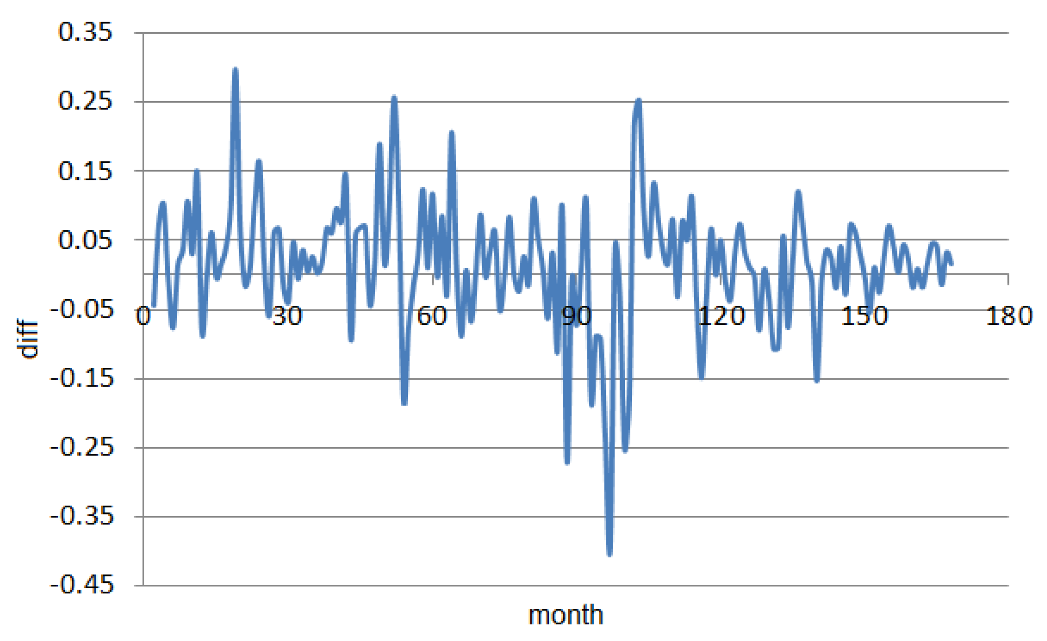
3.3. ARIMA Models for Monthly Series

The best ARIMA models for the monthly series are presented in the following. The lnBET series and subseries present a unit root, so the best models are obtained after taking the first-order difference of the raw series. Therefore, the goodness of fit coefficients will be smaller for the differentiated series (Figure 5) than for the raw series. This aspect should be taken into consideration when comparing the GEP and ARIMA models.

The best ARIMA models for the monthly series are presented in

Table 16. ARIMA models for the monthly series and subseries.

Series	Model Type	Coefficients			The Goodness of Fit Indicators
		AR1	Drift	MA1	RMSE	MSE	MAE	MAPE
S_m	ARIMA (0,1,1) with drift	-	0.2449	0.0156	0.0875	0.0076	0.0621	0.7638
S1_m	ARIMA (0,1,0) with drift	-	0.0422	-	0.0707	0.0050	0.0531	0.7386
S2_m	ARIMA (0,1,0)	-	-	-	0.0755	0.0057	0.0551	0.6203
S3_m	ARIMA (0,1,0) with drift	-	−0.0949	-	0.1508	0.0227	0.1187	1.4401
S4_m	ARIMA (0,1,1)	-	-	0.2774	0.0552	0.0030	0.0432	0.5073
U1_m	ARIMA (1,1,0)	0.2152	-	-	0.0893	0.0080	0.0630	0.7375

. For S1_m, S2_m, and S3_m, they are the differentiated series with or without drift. The models for S_m and S4_m are ARIMA, for which the autoregressive part is missing; for U1_m, it is an ARIMA whose moving average part is absent.

To validate the ARIMA models, the hypothesis that the residual forms a white noise has been tested by using the Anderson–Darling (A–D) test (for normality), the Levene test (for homoskedasticity), and plotting the autocorrelation and partial autocorrelation functions (ACF and PACF). For the last two functions, the lag at which the correlation appears is listed, while p-values (with three decimals) are displayed for the other tests. If the correlation is absent, ‘none’ is inserted in

Table 17. Results of the statistical tests on the residual from ARIMA models for the monthly series.

		A–D	Levene	ACF	PACF	Remark
S_m	ARIMA (0,1,1) with drift	0.000	0.012	4	4	Yes
S1_m	ARIMA (0,1,0) with drift	0.195	0.708	none	none	No
S2_m	ARIMA (0,1,0)	0.335	0.199	none	none	No
S3_m	ARIMA (0,1,0) with drift	0.942	0.179	none	none	No
S4_m	ARIMA (0,1,1)	0.247	0.017	6	6	Yes
U1_m	ARIMA (1,1,0)	0.000	0.000	none	none	Yes

Note. Yes means that the hypothesis that the residual forms a white noise could be rejected.

that summarizes the results.

Among the ARIMA models for the monthly series, only three are correct from a statistical viewpoint, those for S1_m, S2_m, and S3_m. These are kept for comparisons, given that only valid models can be employed for a possible forecast. The GEP models for S_m, S4_m, and U1_m (Table 4 and Table 5) are kept.

Comparing the models for S2_m (Table 4), it results that the GEP one is the best on the test set (showing that the GEP algorithm learned the data well, and applied what it learned on the new dataset). The same is true for S3_m considering all indicators but MAPE, which is slightly higher for S3_m (the test set).

For a fair comparison, the GEP has been run for S1_m, S2_m, and S3_m without dividing the series into two parts, for training and test. It resulted in:

• For S1_m, RMSE = 0.1788, MSE = 0.0320, MAE = 0.0759, MAPE = 1.1035;
• For S2_m, RMSE = 0.09165, MSE = 0.0084, MAE = 0.0638, MAPE = 0.7226;
• For S3_m, RMSE = 0.2200, MSE = 0.0484, MAE = 0.1594, MAPE = 1.8826.

Therefore, in these cases, ARIMA models are the best.

The ARIMA models for the monthly detrended series are presented in

Table 18. ARIMA models for monthly detrended series.

Series	Model Type	Coefficients			The Goodness of Fit Indicators
		AR Coefficients	Drift	MA1	RMSE	MSE	MAE	MAPE
S_md	ARIMA (0,1,1)	-	-	0.2462	0.0875	0.0077	0.0626	111.8606
S1_md	ARIMA (1,0,0) with 0 mean	-	0.7873	-	0.6720	0.4516	0.0530	41.9276
S2_md	ARIMA (1,0,0) with 0 mean	AR1 = 0.6492	-	-	0.0693	0.0048	0.0552	197.9489
S3_md	ARIMA (0,1,0)	-	-	-	0.2260	0.0511	0.1675	65.7451
S4_md	ARIMA (2,0,0)	AR1 = 1.2211 AR2 = −0.3352	-	-	0.0540	0.0029	0.0417	103.3804
U1_md	ARIMA (3,0,1)	AR1 = 2.0902 AR2 = −1.2549 AR3 = 0.1561	-	−0.9868	0.0858	0.0074	0.0610	87.0538

.

Among them, there are an ARMA(3,1) (for U1_d) and three AR (for S1_d, S2_d, and U1_d) models. At first sight, all of them have significantly higher MAPE than the corresponding GEP models (Table 7 and Table 9). Being a non-dimensional indicator, MAPE is most suitable for comparing different kinds of models. Based on this, GEP models are more competitive.

The results of the models’ validation are contained in

Table 19. Results of the statistical tests on the residual from ARIMA models for the monthly detrended series.

Series	Model Type	A–D	Levene	ACF	PACF	Remark
S_md	ARIMA (0,1,1)	0.000	0.001	4	4	Yes
S1_md	ARIMA (1,0,0) with 0 mean	0.248	0.843	none	none	No
S2_md	ARIMA (1,0,0) with 0 mean	0.005	0.032	none	none	Yes
S3_md	ARIMA (0,1,0)	0.089	0.237	none	none	No
S4_md	ARIMA (2,0,0)	0.164	0.012	4	4	Yes
U1_md	ARIMA (3,0,1)	0.005	0.000	none	none	Yes

Note. Yes means that the hypothesis that the residual forms a white noise could be rejected.

. Based on this, only two models (Table 18) should be compared to the GEP ones, S1_md and S3_md. For these series, all the indicators of the GEP models are lower than the corresponding ones for ARIMA. Therefore, the best performances are noticed for all the GEP detrended series.

The ARIMA models for the monthly deseasonalized series are given in

Table 20. ARIMA models for the monthly deseasonalized series.

		Coefficients			The Goodness of Fit Indicators
Series	Model Type	AR1	Drift	MA1	RMSE	MSE	MAE	MAPE
S_ms	ARIMA (0,1,1) with drift	-	0.01564	0.0156	0.0904	0.0080	0.0635	0.7816
S1_ms	ARIMA (0,1,0) with drift	-	0.0424	-	0.0740	0.0055	0.0540	0.0127
S2_ms	ARIMA (0,1,0) with drift	-	0.0156	-	0.0572	0.0033	0.0422	0.4753
S4_ms	ARIMA (0,1,0) with drift		0.0154	-	0.0606	0.0037	0.0431	0.5044
U1_ms	ARIMA (0,1,0)	-	-	-	0.0954	0.0091	0.0654	0.7698

, and the results of their validation are in

Table 21. Results of the statistical tests on the residual from ARIMA models for the monthly deseasonalized series.

Series	Model Type	A–D	Levene	ACF	PACF	Remark
S_ms	ARIMA (0,1,1) with drift	0.942	0.001	4	4	Yes
S1_ms	ARIMA (0,1,0) with drift	0.017	0.723	none	none	Yes
S2_ms	ARIMA (0,1,0) with drift	0.061	0.833	none	none	No
S4_ms	ARIMA (0,1,0) with drift	0.001	0.017	none	none	Yes
U1_ms	ARIMA (0,1,0)	0.000	0.000	1	1	Yes

Note. Yes means that the hypothesis that the residual forms a white noise could be rejected.

. Among the models, only that for S2_ms was validated (the hypothesis that the residual forms a white noise could not be rejected), so only the quality of this model should be discussed. The corresponding goodness of fit indicators in the ARIMA are smaller than those in the GEP model for S2_ms (Table 15). Still, for a relevant comparison of both models, the entire series has been used for building a GEP model. The indicators that characterize it are RMSE = 0.0523, MSE = 0.0027, MAE = 0.0384, MAPE = 0.4237. Therefore, the GEP model is the best one.

Comparison of the ARIMA models for the raw series, the detrended and deseasonalized ones shows that:

• In terms of MAPE, the models for the detrended series are the worst.
• Taking into account RMSE, MSE, and MAE, the raw series models have similar performances with those for the detrended series for all but S3. Still, the model for S2_md is worse than for S2, since the first one does not satisfy the hypotheses on the residuals.
• In terms of MAPE, the ARIMA models for S2_ms and S4_ms are better than those of S2_m and S4_m. Even if the MAPE for S1_ms is smaller than for S1_m, the residual is not white noise, so the first model cannot be considered better than the corresponding one for the raw data series.
• Comparative results have been obtained for U1_m and U1_ms.
• The other goodness of fit indicators generally have comparative values for the rest of the initial and deseasonalized series.

3.4. ARIMA Models for Weekly Series

The same procedure was followed for studying the weekly series. The ARIMA models for the series and the detrended ones are given in

Table 22. ARIMA models for weekly series S_w, S1_w, S2_w, S3_w, S4_w, and U1_w.

Series	Model Type	Coefficients			The Goodness of Fit Indicators
		AR Coef.	Drift	MA Coef.	RMSE	MSE	MAE	MAPE
S_w	ARIMA (1,0,5)	AR1 = −0.9765	-	MA1 = 0.0167 MA2 = −0.8277 MA3 = 0.0373 MA4 = −0.1195 MA5 = −0.0816	0.0373	0.0014	0.0260	0.3219
S1_w	ARIMA (0,1,0) with drift	-	0.0101	-	0.0320	0.0010	0.0242	0.3404
S2_w	ARIMA (0,1,0)	-	0.0041	-	0.0342	0.0012	0.0258	0.2910
S3_w	ARIMA (0,1,0) with drift	-	−0.017	-	0.0681	0.0046	0.0471	0.0012
S4_w	ARIMA (4,1,1) with drift	AR1 = −0.6230 AR2 = 0.1165 AR3 = 0.0737 AR4 = −0.1307	0.0030	MA1 = 0.5924	0.0292	0.0009	0.0208	0.2444
U1_w	ARIMA (3,1,0) with drift	AR1 = 0.0034 AR2 = 0.1779 AR3 = 0.0934	-	-	0.0391	0.0015	0.0267	0.3123

and

Table 23. ARIMA models for detrended weekly series S_wd, S1_wd, S2_wd, S3_wd, S4_wd, and U1_wd.

Series	Model Type	Coefficients			The Goodness of Fit Indicators
		AR	Drift	MA1	RMSE	MSE	MAE	MAPE
S_wd	ARIMA (0,0,1) with 0 mean	-	-	0.2462	0.0875	0.0077	0.0626	111.8606
S1_wd	ARIMA (1,0,0) with 0 mean	-	0.7873	-	0.6720	0.4516	0.0530	41.9276
S2_wd	ARIMA (1,0,0) with 0 mean	AR1 = 0.6492	-	-	0.0693	0.0048	0.0552	197.9489
S3_wd	ARIMA (0,1,0)	-	-	-	0.2260	0.0511	0.1675	65.7451
S4_wd	ARIMA (2,0,0)	AR1 = 1.2211 AR2 = −0.3352	-	-	0.0540	0.0029	0.0417	103.3804
U1_wd	ARIMA (3,0,1)	AR1 = 2.0902 AR2 = −1.2549 AR3 = 0.1561	-	−0.9868	0.0858	0.0074	0.0610	87.0538

.

The output of the tests for validating the models is contained in

Table 24. Tests of the residuals in ARIMA models for the weekly series S_w, S1_w, S2_w, S3_w, S4_wd, and U1_w.

Series	Model Type	A–D	Levene	ACF	PACF	Remark
S_w	ARIMA (1,0,5)	0.000	0.000	none	none	Yes
S1_w	ARIMA (0,1,0) with drift	0.004	0.130	11	11	Yes
S2_w	ARIMA (0,1,0)	0.117	0.287	none	none	No
S3_w	ARIMA (0,1,0) with drift	0.000	0.285	2	3	Yes
S4_w	ARIMA (4,1,1) with drift	0.000	0.000	none	none	Yes
U1_w	ARIMA (3,1,0) with drift	0.000	0.000	12	12	Yes

Note. Yes means that the hypothesis that the residual forms a white noise could be rejected.

and

Table 25. Tests of the residuals in ARIMA detrended models for weekly series S_wd, S1_wd, S2_wd, S3_wd, S4_wd, and U1_wd.

Series	Model Type	A–D	Levene	ACF	PACF	Remark
S_w	ARIMA (0,0,1) with 0 mean	0.000	0.000	12	12	Yes
S1_w	ARIMA (1,0,0) with 0 mean	0.003	0.146	none	11	Yes
S2_w	ARIMA (1,0,0) with 0 mean	0.087	0.317	10	11	Yes
S3_w	ARIMA (0,1,0)	0.000	0.352	none	none	Yes
S4_w	ARIMA (2,0,0)	0.000	0.000	none	none	Yes
U1_w	ARIMA (3,0,1)	0.000	0.000	12	11	Yes

Note. Yes means that the hypothesis that the residual forms a white noise could be rejected.

.

Table 24 shows that all but the ARIMA model for S2_w do not satisfy the hypothesis that the residual series form a white noise.

To compare the models for S2_w, the GEP algorithm has been run without dividing the series into training and test. The following values of the indicators have been obtained: RMSE = 0.0477, MSE = 0.0023, MAE = 0.0285, MAPE = 0.3222 (higher than the corresponding values in the ARIMA model). Therefore, ARIMA performs better than GEP only on S2_w.

Table 25 shows that the ARIMA models for the detrended weekly series cannot be validated. Furthermore, MAPE is extremely high by comparison to those of the GEP models for the same series, and of ARIMA models for the raw weekly data. So, the trend removal does not lead to the quality augmentation.

4. Conclusions

Financial time series are characterized by nonlinearity and high variability, often accompanied by heteroskedasticity and non-stationarity, which make the deterministic methods unsuitable for modeling such series. Different stochastic models rely on restrictive assumptions on the data generating processes. The artificial intelligence methods do not impose such restrictions, making them good options when other kinds of algorithms cannot be used, or satisfactory models cannot be found by other approaches.

Despite their advantages, the relationship between the statistical properties of the data series—normality, homoscedasticity, autocorrelation, stationarity, and the trend existence—and the quality of the models built for the series utilizing AI techniques was not investigated. Knowledge on the performances of different algorithms applied on time series with the same statistical properties would eliminate some modeling options, and reduce the time of searching for the appropriate approach. Such modeling is suitable not only for financial time series but for other fields as well, according to the statistical characteristics of a series.

Therefore, in this article, we built GEP and ARIMA models for lnBET series and subseries, to determine if the statistical properties are connected to the goodness of fit of such models. The modeling results show that:

(1)

The normality and homoskedasticity do not have a major influence on the models’ performances;

(2)

The trend removal results in better GEP models;

(3)

The seasonality elimination does not lead to an improvement of the modeling quality.

(4)

The trend removal results in worse ARIMA models;

(5)

Generally, GEP performed better than ARIMA on the study series.

Remark (1) does not seem surprising, since we are dealing with point forecasts and performance measures of conditional location parameters of the conditional density.

The first three findings are in concordance with the results from [14], which refers to GRNN models.

The study should be extended on simulated and other real data series for collecting more evidence on the connection between the models’ performances and the series statistical characteristics.

References

1. Sinclair, T.M.; Stekler, H.O.; Kitzinger, L. Directional forecasts of GDP and inflation: A joint evaluation with an application to Federal Reserve predictions. Appl. Econ. 2008, 40, 2289–2297. [Google Scholar] [CrossRef]
2. Wagner, N.; Michalewicz, Z.; Khouja, M.; Mcgregor, R.R. Time series forecasting for dynamic environments: The dyfor genetic program model. IEEE Trans. Evol. Comput. 2007, 11, 433–452. [Google Scholar] [CrossRef] [Green Version]
3. Box, G.; Jenkins, G. Time Series Analysis: Forecasting and Control; Holden-Day: San Francisco, FA, USA, 1970. [Google Scholar]
4. Li, Z.; Han, J.; Song, Y. On the forecasting of high-frequency financial time series based on ARIMA model improved by deep learning. J. Forecast. 2020, 39, 1081–1097. [Google Scholar] [CrossRef]
5. Pahlavani, M.; Roshan, R. The Comparison among ARIMA and hybrid ARIMA-GARCH Models in Forecasting the Exchange Rate of Iran. Int. J. Bus. Dev. Stud. 2015, 7, 31–50. [Google Scholar]
6. Hamilton, J. Time Series Analysis; Princeton University Press: Princeton, NJ, USA, 1994. [Google Scholar]
7. Kuan, C.-M. Lecture on the Markov switching model. Inst. Econ. Acad. Sin. 2002, 8, 1–30. [Google Scholar]
8. Harvey, A.C.; Ruiz, E.; Shephard, N. Multivariate stochastic variance models. Rev. Econ. Stud. 1994, 61, 247–264. [Google Scholar] [CrossRef] [Green Version]
9. Gray, S.F. Modeling the conditional distribution of interest rates as a regime switching process. J. Financ. Econ. 1996, 42, 27–62. [Google Scholar] [CrossRef]
10. Chatfield, C. Time Series Forecasting; Chapman and Hall Text in Statistical Science: London, UK, 2000. [Google Scholar]
11. Lee, C.F.; Chen, G.-M.; Rui, O.M. Stock returns and volatility on China’s stock markets. J. Fin. Res. 2014, 24, 523–543. [Google Scholar] [CrossRef]
12. Lo, A.W. The Adaptive Markets Hypothesis: Market Efficiency from an evolutionary perspective. J. Portf. Manag. 2004, 30, 15–29. [Google Scholar] [CrossRef]
13. Bărbulescu, A.; Băutu, E. A hybrid approach for modeling financial time series. Int. Arab J. Inf. Technol. 2012, 9, 327–335. [Google Scholar]
14. Bărbulescu, A. Do the time series statistical properties influence the goodness of fit of GRNN models? Study on financial series. Appl. Stoch. Model. Bus. 2018, 34, 586–596. [Google Scholar] [CrossRef]
15. Simian, D.; Stoica, F.; Bărbulescu, A. Automatic Optimized Support Vector Regression for Financial Data Prediction. Neural Comput. Appl. 2020, 32, 2383–2396. [Google Scholar] [CrossRef]
16. Chen, S. Genetic Algorithms and Genetic Programming in Computational Finance; Kluwer Academic Publishers: Amsterdam, The Nederlands, 2002. [Google Scholar]
17. Karathanasopoulos, A.; Sermpinis, G.; Laws, J.; Dunis, C. Modelling and trading the Greek stock market with Gene Expression and Genetic Programing algorithms. J. Forecast. 2014, 33, 596–610. [Google Scholar] [CrossRef] [Green Version]
18. Peng, X. TSVR: An efficient twin support vector machine for regression. Neural Netw. 2010, 23, 365–372. [Google Scholar] [CrossRef] [PubMed]
19. Cao, L.; Tay, F.E.H. Financial forecasting using support vector machines. Neural Comput. Appl. 2001, 10, 184–192. [Google Scholar] [CrossRef]
20. Emad, W.S.; Danil, V.P.; Donald, C.W. Comparative study of stock trend prediction using time delay, recurrent and probabilistic neural networks. IEEE Trans. Neural Netw. 1998, 9, 1456–1470. [Google Scholar]
21. Lin, C.T.; Prasad, M.; Saxena, A. An Improved Polynomial Neural Network Classifier Using Real Coded Genetic Algorithm. IEEE Trans. Syst. Man Cybern. Syst. 2015, 45, 1389–1401. [Google Scholar] [CrossRef]
22. Koza, J.R. Genetic programming as a means for programming computers by natural selection. Stat. Comput. 1994, 4, 87–112. [Google Scholar] [CrossRef]
23. Ferreira, C. Gene Expression Programming: Mathematical Modeling by an Artificial Intelligence, 2nd ed.; Springer: Berlin/Heidelberg, Germany, 2006. [Google Scholar]
24. Huang, C.H.; Yang, C.B.; Chen, H.H. Trading strategy mining with gene expression programming. In Proceedings of the 2013 International Conference on Applied Mathematics and Computational Methods in Engineering, Rhodes Island, Greece, 21–27 September 2013; pp. 37–42. [Google Scholar]
25. Chen, H.H.; Yang, C.B.; Peng, Y.H. The trading on the mutual funds by gene expression programming with Sortino ratio. Appl. Soft Comput. 2014, 15, 219–230. [Google Scholar] [CrossRef]
26. Lee, C.-H.; Yang, C.-B.; Chen, H.-H. Taiwan stock investment with gene expression programming. Procedia Comput. Sci. 2014, 35, 137–146. [Google Scholar] [CrossRef] [Green Version]
27. Sermpinis, G.; Laws, J.; Karathanasopoulos, A.; Dunis, C. Forecasting and trading the EUR/USD exchange rate with Gene Expression and Psi Sigma Neural Networks. Expert Syst. Appl. 2012, 31, 8865–8877. [Google Scholar] [CrossRef]
28. Bărbulescu, A.; Dumitriu, C.S. Artificial intelligence models for financial time series. Ovidius Univ. Ann. Econ. Sci. Ser. 2021, in press. [Google Scholar]
29. Ariton, V.; Palade, V.; Postolache, F. Combined deep and shallow knowledge in a unified model for diagnosis by abduction. EuroEconomica 2008, 1, 33–42. [Google Scholar]
30. Dragomir, F.L. Modeling Resource in E-Commerce. In Proceedings of the 10th International Conference on Knowledge Management: Projects, Systems and Technologies, Bucharest, Romania, 23–24 November 2017; Security and Defence Faculty “Carol I” National Defence University: Bucharest, Romania, 2017; pp. 38–41. [Google Scholar]
31. Dragomir, F.L. Models of Digital Markets. In Proceedings of the 10th International Conference on Knowledge Management: Projects, Systems and Technologies, Bucharest, Romania, 23–24 November 2017; Security and Defence Faculty “Carol I” National Defence University: Bucharest, Romania, 2017; pp. 47–51. [Google Scholar]
32. Bărbulescu, A.; Dumitriu, C.S. Markov Switching Model for Financial Time Series. Ovidius Univ. Ann. Econ. Sci. Ser. 2021, in press. [Google Scholar]
33. Postolache, F.; Bumbaru, S.; Ariton, V. Complex systems virtualization in the current’s economical context. EuroEconomica 2010, 3, 29–50. [Google Scholar]
34. Bucharest Stock Exchange. Available online: http://www.bvb.ro (accessed on 10 April 2019).
35. Bucharest Exchange Trading. Available online: www.bvb.ro/info/indices/2017/2017.10.10%20-%20BET%20Factsheet.pdf (accessed on 10 April 2019).
36. Gel, Y.R.; Gastwirth, J.L. A robust modification of the Jarque-Bera test of normality. Econ. Lett. 2008, 99, 30–32. [Google Scholar] [CrossRef]
37. Razali, N.M.; Yap, B.W. Power comparisons of Shapiro–Wilk, Kolmogorov–Smirnov, Lilliefors and Anderson–Darling tests. J. Stat. Model. Anal. 2011, 2, 21–33. [Google Scholar]
38. Levene, H. Robust Test for Equality of Variances. In Contributions to Probability and Statistics: Essays in Honor of Harold Hotelling; Olkin, I., Ed.; Stanford University Press: Palo Alto, CA, USA, 1960; pp. 278–292. [Google Scholar]
39. Gibbons, J.D.; Chakraborti, S. Nonparametric Statistical Inference, 4th ed.; Marcel Dekker: New York, NY, USA, 2003. [Google Scholar]
40. Wald, A.; Wolfowitz, J. On a test whether two samples are from the same population. Ann. Math. Stat. 1940, 11, 147–162. [Google Scholar] [CrossRef]
41. Brockwell, P.J.; Davis, R.A. Introduction to Time Series and Forecasting; Springer: New York, NY, USA, 2002. [Google Scholar]
42. Kendall, M.G. Rank Correlation Methods, 5th ed.; Oxford University Press: London, UK, 1990; pp. 56–80. [Google Scholar]
43. Dickey, D.A.; Fuller, W.A. Distribution of the estimators for autoregressive time series with a unit root. J. Am. Stat. Assoc. 1979, 74, 427–431. [Google Scholar]
44. Phillips, P.C.B.; Perron, P. Testing for a unit root in time series regression. Biometrika 1988, 75, 335–346. [Google Scholar] [CrossRef]
45. Kwiatkowski, D.; Phillips, P.C.B.; Schmidt, P.; Shin, Y. Testing the null hypothesis of stationarity against the alternative of a unit root. J. Econ. 1992, 54, 159–178. [Google Scholar] [CrossRef]
46. Pettitt, A.N. A non-parametric approach to the change-point problem. Appl. Stat. 1979, 28, 126–135. [Google Scholar] [CrossRef]
47. Hawkins, D.M.; Olwell, D.H. Cumulative Sum Charts and Charting for Quality Improvement; Springer: New York, NY, USA, 1998. [Google Scholar]
48. Gedikli, A.; Aksoy, H.; Unal, N.E.; Kehagias, A. Modified dynamic programming approach for offline segmentation of long hydrometeorological time series. Stoch. Environ. Res. Risk Assess. 2010, 24, 547–557. [Google Scholar] [CrossRef]
49. Bărbulescu, A. Studies on Time Series. Applications in Environmental Sciences; Springer: New York, NY, USA, 2016. [Google Scholar]
50. Diebold, F.X.; Mariano, R.S. Comparing the predictive accuracy. J. Bus. Econ. Stat. 1995, 13, 253–263. [Google Scholar]
Figure 1. BET monthly (left-hand side) and weekly series (right-hand side).
Mathematics 09 01853 g001
Figure 2. The best model for S1_m (with lag 1 regressor) when a linear trend was removed.
Mathematics 09 01853 g002
Figure 3. The best model for S4_ms (with lag 1 regressor).
Mathematics 09 01853 g003
Figure 4. The weekly series and subseries.
Mathematics 09 01853 g004
Figure 5. The monthly differentiated series.
Mathematics 09 01853 g005