Abstract
Recently, there seems to be an increasing amount of interest in the use of the tail conditional expectation (TCE) as a useful measure of risk associated with a production process, for example, in the measurement of risk associated with stock returns corresponding to the manufacturing industry, such as the production of electric bulbs, investment in housing development, and financial institutions offering loans to small-scale industries. Companies typically face three types of risk (and associated losses from each of these sources): strategic (S); operational (O); and financial (F) (insurance companies additionally face insurance risks) and they come from multiple sources. For asymmetric and bounded losses (properly adjusted as necessary) that are continuous in nature, we conjecture that risk assessment measures via univariate/bivariate Kumaraswamy distribution will be efficient in the sense that the resulting TCE based on bivariate Kumaraswamy type copulas do not depend on the marginals. In fact, almost all classical measures of tail dependence are such, but they investigate the amount of tail dependence along the main diagonal of copulas, which has often little in common with the concentration of extremes in the copula’s domain of definition. In this article, we examined the above risk measure in the case of a univariate and bivariate Kumaraswamy (KW) portfolio risk, and computed TCE based on bivariate KW type copulas. For illustrative purposes, a well-known Stock indices data set was re-analyzed by computing TCE for the bivariate KW type copulas to determine which pairs produce minimum risk in a two-component risk scenario.
1. Introduction
In practice, insurance companies retain amounts of capital from which they can draw upon, in the (unfavorable) event that premium revenues become inadequate to pay out claims. The appropriate determination of such amounts is quite a difficult task. At the outset, the procedure should be able to resolve with accuracy the underlying probability distribution of the losses that it is experiencing. As a next step, a judicious choice/selection needs to be made in terms of a risk measure (or a set of risk measures) that is expected to perform in the most efficient way. For a detailed mathematical derivation in the context of the TCE for a continuous random variable Y that indicates the loss incurred, see [1] and the references cited therein. Consider a loss random variable Y having a density (and distribution) function given by (and , respectively). Then, the tail function of Y is It can be considered as the value of a total claim for an actuary firm in the context of a portfolio of investments made by a single individual or by the entire firm as a whole.
The tail conditional expectation (henceforth, in short, TCE) is defined as
This can be interpreted as the mean of very bad losses. It provides an average amount of the tail of the distribution which is usually based on the p-th quantile of the loss distribution with the property The associated TCE is given by
where
There exists a vast literature on the evaluation of TCE of random losses corresponding to several well-known probability distributions (mostly in the continuous case for the obvious reason as mentioned earlier due to [1]). For example, TCEs for the univariate and multivariate normal family have been extensively discussed in [2] However, a major drawback to this is that all members of the elliptical family are symmetric. Arguably, the first work which this author can cite in investigating the tail conditional expectation risk measure in non-symmetric loss distributions domain is by [3]. However, in the context of bounded dependent risks (and associated losses), it is desirable to have available flexible probability models with analytic expressions for the corresponding marginal distributions as well as its’ quantile functions. Noticeably, in the case of unbounded losses, it might be useful on certain occasions to transform the risks to take on values in the interval in order to take advantage of the flexible arrays of bivariate models that exist in the literature, such as beta and Kumaraswamy. In this paper, we consider a more useful two-parameter absolutely continuous probability distribution called Kumaraswamy (1980) distribution. The Kumaraswamy distribution (henceforth, in short, the distribution) on the interval , has its probability density function (p.d.f.) and its c.d.f. with two shape parameters and given by
If a random variable Y has (3) as its density, then we will write The KW distribution enjoys some interesting properties which establishes its flexibility in modeling bounded data—for more details, see [4].
Because of these striking advantages, it is imperative to explore and develop the expressions for TCE when the underlying losses have univariate/bivariate and multivariate Kumaraswamy models. Let us suppose that an actuary firm operates n lines of business and the risk managers are interested in knowing the amount of risk hidden in line The answer to this query would be to find the associated TCE. Then, the allocation of the ℓ-th line of business of the actuary firm on its total risk capital will be:
where Certainly, due to the additive property of conditional expectation, the sum of all marginal risks is equal to the total risk measure for the whole company, meaning that:
One important thing to remember is that tail conditional expectations arising from each individual components do not add up to the TCE in totality. This is because:
Alternatively, we may write this as
The rest of the paper is organized as follows. In Section 2, we provide expressions for tail conditional expectation when the underlying loss distribution is a continuous and univariate Kumaraswamy distribution. Section 3 provides portfolio risk evaluation with TCE for non-negative independent losses, under the KW distributional assumption.
In Section 4, we derive the representation of TCE in the context of various dependent bivariate Kumaraswamy distributions. In Section 5, we provide a copula-based representation of TCE based on several bivariate Kumaraswamy type copulas. For illustrative purposes, a well-known financial (European stock indices data for a specific time period) is considered to compute TCE measures based on bivariate KW type copulas and to determine the lowest risk on a two-component risk scenario in Section 6. Some concluding remarks are presented in Section 7.
2. TCE Formula Based on Univariate Kumaraswamy Distribution
Let us consider Kumaraswamy distributed loss random variable Y with two shape parameters as in (3). Let u be such that and let denote the u-th quantile of the distribution of which in this case is Then, we have the following theorem which represents the expression of TCE related to univariate Kumaraswamy loss.
Theorem 1.
Let Then, the tail conditional expectation of Y is given by
Proof.
Clearly, Therefore:
Hence, the proof. □
3. Portfolio Risk Evaluation with TCE for Non-Negative Independent Losses
In the case of uncertainty arising from different resources, it is quite legitimate to ask how to break down the total level of uncertainty to these sources. Let us assume that the total loss is given by where each represents the claim arising from actuarial firm-related business. Evidently, from [2] (and the references cited therein), and using the result on the additivity of expectation, the tail conditional expectation allows for a natural decomposition of the total loss:
TCE-based allocation formulas for symmetric distributions, having an elliptical dependence structure, were studied in [5]. It is well established that under the assumption of non-negative, asymmetric risk portfolios, the associated computation of TCE is different than the cases where the non-negative risks are symmetric. Then, note that the distribution function of the convolution of two independent non-negative random variables X and Y with support on may be written as
Then, we use the following Lemma (see Lemma p. [6] for details) which represents an expression for the allocation strategy covering non-negative risks in the most general form:
Then, we consider the expression for TCE for non-negative independent losses when the underlying losses are Kumaraswamy (in the bivariate case, ) with the following assumptions:
- and are independent.
We make a note here that one may obtain (using (8)) the denominator of (9), which can be written as
We conjecture here that it is possible to extend this idea to the multivariate Kumaraswamy cases, despite their computational complexity involving special functions. Then, we consider the following Lemma which represents the distribution of the sum of two independent Kumaraswamy distributions.
Lemma 1.
Let us define with and that they are independent. The cumulative distribution function (c.d.f.) of the sum denoted by will be:
Proof.
The cumulative distribution function of S will be:
In our case, Therefore, from (8), we have:
after some algebra. Then, we state the following Theorem which represents the contribution of the marginal loss (say), given that the aggregate risk S is bigger than any shortfall □
Theorem 2.
If the marginal loss and with S defined earlier, then:
Proof.
Since,
Again, Therefore, the integral in the numerator in (9) will be:
after some algebraic simplification. Our result immediately follows by substituting (14) and (13) in (9). Similarly, one can obtain an analogous expression for which will be:
Hence, the expression for TCE for non-negative independent losses when the underlying losses are Kumaraswamy (in the bivariate case) will be:
where the expressions for individual TCE are provided in (12) and (15) and can be obtained by using (10) and doing some standard algebraic computation. □
4. TCE for Dependent Bivariate Kumaraswamy Distributions
It is more practical to consider the dependent risk scenario. We consider two particular bivariate dependent Kumaraswamy models, namely the Dirichlet bivariate and the Libby–Novick–Jones–Olkin–Liu bivariate Kumaraswamy distribution (for details, see [7]).
4.1. The Dirichlet Bivariate Kumaraswamy Model
The corresponding joint density is of the form:
The marginal densities are, by construction, of the Kumaraswamy type. Thus:
and:
Note that, here, and are dependent (for details, see [7]). Then, using known results for the Beta and the Dirichlet distributions, we may verify that:
Theorem 3.
Proof.
We have:
after some algebraic simplification.
Then, we consider the numerator integral of (9) in this case, which is given by
after some algebraic simplification and successive expansion. Consequently, the expression for will be obtained by substituting (18) in (9). Similarly, one can obtain an analogous expression for which will be given by
Hence, the expression of TCE in the bivariate Dirichlet Kumaraswamy distribution will be given by
where the conditional expectations are given in (16) and (19). □
4.2. The Libby–Novick–Jones–Olkin–Liu Bivariate Kumaraswamy Model
The corresponding joint density is of the form:
From [4], p. 236:
Furthermore, the marginal distribution of will be:
Similarly:
In this case, the associated c.d.f. will be:
where:
where the incomplete beta function.
Therefore:
As before, one can obtain from (10) on using (21) and marginal survival functions of and , which are available in closed form in this case.
Then, we consider the numerator integral of (9) in this case, which is given by
after some algebraic simplification and successive expansion. Consequently, the expression for will be obtained by substituting (22) in (9) and will be given by
Similarly, one can obtain an analogous expression for which will be given by
where:
Hence, the expression of TCE in the bivariate dependent LNJOL Kumaraswamy distribution will be given by
where the individual conditional expectations are given previously.
5. Copula-Based Conditional Tail Expectation for Kumaraswamy Dispersion Models
In a risk assessment paradigm, several useful risk evaluation measures have been suggested, such as the value at risk (VaR), the tail conditional expectation (TCE), the distorted risk measures (DRM), and distortion risk measures based on copula (DRMC, in short)—for pertinent reference in this context, see [8] and the references cited therein. For a real number in the TCE of a risk Y will be:
where is the th order quantile corresponding to the cumulative distribution function (c.d.f.) In practice, the expectation of Y is computed when the conditional event is fixed (for example, to be equal to 90% or 95%). Then, let us assume that we encounter with a bivariate random risk (or losses) represented by It is quite obvious that the TCE of is unrelated to Consequently, if we want to control the overflow of the two risks and at the same time, the above formula of TCE does not provide a satisfactory remedy to this problem; therefore, one might require a separate formula of TCE which takes into account the excess of the two risks and Then, we deal with the amount:
If the bivariate random risks are independent in nature, then the expression in (23) only defined the TCE of a univariate risk, for a fixed conditional event Therefore, the case of independence is of much importance. Recently, dependence is beginning to play a vital role in portfolio risk modeling. For relative merits and demerits between the assumption(s) of independent and dependent risks, see, [9] and the references cited therein. However, in reality, the dependence assumption appears to be more reasonable. The above risk measure in (24) is known as the copula conditional tail expectation (CCTE); for details, see [10]. Let be the market-determined values of a portfolio of assets over m periods, and be the negative log return (loss) over the t-th period. Then, given a positive number , a very small quantity (almost close to 0), the VaR of Y at the confidence level will be:
For a detailed study on the computation of VaR used in the pure copula method, we refer the interested reader to [11]. Then, we state the following proposition (according to Proposition (p. 85, [9]) which represents a useful formula to compute the copula-based CCTE (equivalently, TCE in our terminology) given as follows. However, we slightly modified the original proposition (which was not clearly mentioned in [9]) to make it a correct one.
Proposition 1.
Let be a bivariate absolutely continuous random variable with joint distribution function represented by the copulaAssuming thathas a finite mean and c.d.f.Then, for a fixed θ and for allthe copula conditional tail expected ofis given by
whereis the quantile function of Then, we consider two particular dependent bivariate Kumaraswamy type copulas (for details on these bivariate KW type copulas, see [12]).
- Bivariate Kumaraswamy (type-I) CopulaThe associated copula density will be:
- Bivariate Kumaraswamy (type-II) CopulaFrom [13] p. 6, the bivariate copula:for any . Then, the associated density will be:
6. Application
In this section, we re-analyze a data set involving 500 observations from four European stock indices return series calculated by during the period from July 1991 to June 1993, a data set which is available in “QRM and datasets packages” in R software. This data set was independently analyzed by [10] assuming a two-parameter Gamma distribution. This data set involves a record on everyday closing prices of prime European stock indices, for example: Germany DAX (Ibis), Switzerland SMI, France CAC and UK FTSE. Note that the information collected from these data are on weekdays, during which usual business activities can be observed. We conjecture at this point that copulabased bivariate KW type models would be reasonable for computing TCE measures and determine the minimum risk for two-component risks. In Table 1, the estimated value of Kendall’s tau between the four Market Index returns as a measure of dependence are given in tabular form. With the assumption that bivariate KW (Type I) copula and bivariate KW (Type II) copula represent our four dependence structures, we obtain the estimated values of the dependence parameters for the 6 pairwise distribution functions, as reported in Table 2 and Table 3, respectively.

Table 1.
Kendall’s tau matrix estimates from four European stock indices returns.
Table 2.
Fitted copula parameter for the bivariate KW (Type I) copula.
Table 3.
Fitted copula parameter for the bivariate KW (Type II) copula.
The smallest value in Table 4 produces the lowest risk. Consequently, the less risky paired components are: and where X is the target risk and Y is the associated risk. We also utilized bivariate Gaussian copula (Ref: https://arxiv.org/pdf/0912.2816.pdf, Equation (2.1), (accessed on 15 December 2009)) to compute TCE to determine the minimum risk for a two-component risk scenario. The results are given in Appendix A. From the results, it is evident that by using the Gaussian copula (for several of the estimated choices of the dependence parameter from the above data), the results are less efficient in the sense that the computed TCE risk measures, in several cases (see Table A2, values, for example, (i) row 5, columns 1–3; (ii) row 4, column 4), which have quite large values. Therefore, one cannot make a decision on the minimum risk(s) for this particular data set based on a Gaussian copula. The reason being for this particular data set that it must be the case that the measures of tail dependence (as quantified by the TCE) are heavily dependent on the marginal distributions, which is contrary to the general perception that “When it comes to quantifying the extent of tail dependence, it is generally agreed that measures of tail dependence must be independent of the marginal distributions of the risks but rather solely copula-dependent” (for details, see [6] and the references cited there in). Consequently, the efficiency of KW-based bivariate copula in terms of TCE measures is established in this context. The results corresponding to the Gaussian copula are given in the Appendix A.
Table 4.
TCE Risk measures for and with bivariate Gaussian copula with (left panel) and bivariate Gaussian copula with (right panel).
7. Conclusions
In this paper, we focused our attention on the computation of TCE when the underlying portfolio losses are from a bounded risk (individually and/or component wise for two and higher dimensions), preferably following a univariate KW distribution. We also considered independent and dependent bivariate KW distribution for a two-dimensional portfolio risk and computed the associated TCE. This class of distributions may serve as error distribution for generalized linear models in the sense developed by [14]. In this study, we explored the possibility of having bivariate KW-based copulas that may be utilized for assessing risk (in the form of TCE measures), especially in situations where bounded losses are available and easy to deal with. In addition, for illustrative purposes, based on a real-life data set (stock market data), we computed CCTE measures based on two types of bivariate KW copulas and identified which pairs would provide less risk based on the computed values of the associated TCE. Anyone believing that their data (absolutely continuous in nature) are a distributed bivariate Kumaraswamy model as considered herein may find this work self-contained.
Author Contributions
Conceptualization, I.G.; formal analysis, I.G.; investigation, I.G. and F.J.M.; methodology, I.G.; Validation, I.G. and F.J.M.; Writing—original draft, I.G.; Writing—review and editing, I.G. and F.J.M. All authors have read and agreed to the published version of the manuscript.
Funding
This work was partially supported by the Fundação para a Ciência e a Tecnologia (Portuguese Foundation for Science and Technology) through the project UIDB/00297/2020 (Centro de Matemática e Aplicações).
Institutional Review Board Statement
Not applicable.
Informed Consent Statement
Not applicable.
Data Availability Statement
Not applicable.
Conflicts of Interest
The authors declare no conflict of interest.
Appendix A
For the European stock indices data, as indicated previously, for illustrative purposes, we considered the bivariate normal copula as a probable candidate to identify the less risky paired components. It is defined as follows:
where is the joint distribution function of a bivariate normal vector with zero means, unit variances and correlation Table A1 summarizes the estimate of the copula parameter for the six pairs of data when fitted with the bivariate normal copula.
Table A1.
Fitted copula parameter for the Gaussian copula.
Table A1.
Fitted copula parameter for the Gaussian copula.
| Variable | DAX | SMI | CAC | FTSE |
|---|---|---|---|---|
| DAX | 1 | 0.8649 | 0.5893 | 0.3231 |
| SMI | 0.8649 | 1 | 0.4529 | 0.8524 |
| CAC | 0.5893 | 0.4529 | 1 | 0.6372 |
| FTSE | 0.3231 | 0.8524 | 0.6372 | 1 |
In Table A2, we calculated for a fixed level the TCE risk measures for all the cases for the bivariate Gaussian copula, the results of which are summarized in Table 4.
Table A2.
TCE risk measures for and with bivariate Gaussian copula left panel (with ) and right panel (with ).
Table A2.
TCE risk measures for and with bivariate Gaussian copula left panel (with ) and right panel (with ).
| Variable | DAX | SMI | CAC | FTSE |
|---|---|---|---|---|
| DAX | — | 19.4533 | 25.6072 | 26.1129 |
| SMI | 29.4561 | — | 23.4038 | 22.6875 |
| CAC | 34.6823 | 18.6045 | — | 28.5331 |
| FTSE | 32.5709 | 27.4533 | 26.7138 | — |
For illustrative purposes, we provided Figure A1 on TCE measures computed from bivariate KW (type-I) copula, bivariate KW (type-II) copula, and the bivariate Gaussian copula for two selected values of = 0.9, 0.95. From these two graphs, it can be observed that for the stock return data, Gaussian copula-based TCE has more dependence on the marginals, and as a consequence, it fails to capture the tail conditional risk for several paired stock indices to obtain which pairs have the minimum risk. In these graphs, the X axis represents the values of the parameters of the KW distribution (i.e., both a and b, which are rotated from the starting value from to . The reason being, for all the paired data sets, the estimated values of the two parameters for the two parameter KW distribution, and estimated values of a and b appear to be the following:
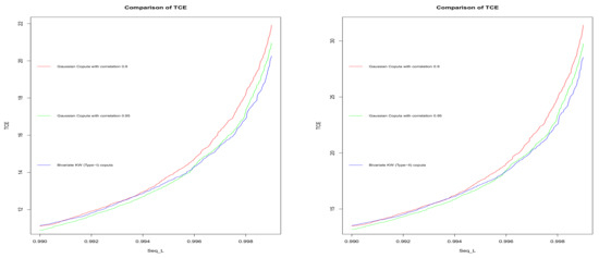
Figure A1.
Comparison of TCE measures based on the bivariate KW (type-I) copula, a bivariate KW (type-II) copula with a bivariate Gaussian copula for the selected parameter choices of KW distribution obtained from the stock return data.
References
- Artzner, P.; Delbaen, F.; Eber, J.M.; Heath, D. Coherent Measures of Risk. Math. Financ. 1999, 9, 203–228. [Google Scholar] [CrossRef]
- Panjer, H.H.; Jing, J. Solvency and Capital Allocation. Research Report 01-14; Institute of Insurance and Pension Research, University of Waterloo: Waterloo, ON, Canada, 2001. [Google Scholar]
- Landsman, Z.; Valdez, E. Tail Conditional Expectation for Exponential Dispersion Models. ASTIN Bull. J. IAA 2005, 35, 189–209. [Google Scholar] [CrossRef] [Green Version]
- Arnold, B.C.; Ghosh, I. Bivariate beta and Kumaraswamy Models developed using the Arnold-Ng bivariate beta distribution. Revstat Stat. J. 2017, 5, 223–250. [Google Scholar]
- Landsman, Z.; Valdez, E. Tail Conditional Expectation for Elliptical Distributions. N. Am. Actuar. J. 2003, 7, 55–71. [Google Scholar] [CrossRef] [Green Version]
- Furman, E.; Kuznetsov, A.; Su, J.; Zitikis, R. Tail dependence of the Gaussian copula revisited. Insur. Math. Econ. 2016, 69, 97–103. [Google Scholar] [CrossRef] [Green Version]
- Arnold, B.C.; Ghosh, I. Some alternative Bivariate Kumaraswamy models. Commun. Stat. Theory Methods 2017, 46, 9335–9354. [Google Scholar] [CrossRef]
- Lin, F.; Peng, L.; Xie, J.; Yang, J. Stochastic distortion and its transformed copula. Insur. Math. Econ. 2018, 79, 148–166. [Google Scholar] [CrossRef]
- Brahim, B.; Fatah, B.; Djabrane, Y. Copula conditional tail expectation for multivariate financial risks. Arab. J. Math. Sci. 2018, 24, 82–100. [Google Scholar] [CrossRef]
- Brahimi, B. Involving copula functions in conditional tail expectation. arXiv 2012, arXiv:1205.4345. [Google Scholar]
- Ouyang, Z.-S.; Liao, H.; Yang, X.-Q. Modeling dependence based on mixture copulas and its application in risk management. Appl. Math. J. Chin. Univ. 2009, 24, 393–401. [Google Scholar] [CrossRef]
- Ghosh, I.; Ray, S. Some alternative bivariate Kumaraswamy type distributions via copula with application in risk management. J. Stat. Theory Pract. 2016, 10, 693–706. [Google Scholar] [CrossRef]
- Ghosh, I. Bivariate Kumaraswamy Models via Modified FGM Copulas: Properties and Applications. J. Risk Financ. Manag. 2017, 10, 19. [Google Scholar] [CrossRef] [Green Version]
- Nelder, J.A.; Wedderburn, R.W. Generalized linear models. J. R. Stat. Soc. Ser. A 1972, 135, 370–384. [Google Scholar] [CrossRef]
Publisher’s Note: MDPI stays neutral with regard to jurisdictional claims in published maps and institutional affiliations. |
© 2021 by the authors. Licensee MDPI, Basel, Switzerland. This article is an open access article distributed under the terms and conditions of the Creative Commons Attribution (CC BY) license (https://creativecommons.org/licenses/by/4.0/).