Abstract
Artificial neural network (ANN) inherently cannot explain in a comprehensible form how a given decision or output is generated, which limits its extensive use. Fuzzy rules are an intuitive and reasonable representation to be used for explanation, model checking, and system integration. However, different methods may extract different rules from the same ANN. Which one can deliver good quality such that the ANN can be accurately described by the extracted fuzzy rules? In this paper, we perform an empirical study on three different rule extraction methods. The first method extracts fuzzy rules from a fuzzy neural network, while the second and third ones are originally designed to extract crisp rules, which can be transformed into fuzzy rules directly, from a well-trained ANN. In detail, in the second method, the behavior of a neuron is approximated by (continuous) Boolean functions with respect to its direct input neurons, whereas in the third method, the relationship between a neuron and its direct input neurons is described by a decision tree. We evaluate the three methods on discrete, continuous, and hybrid data sets by comparing the rules generated from sample data directly. The results show that the first method cannot generate proper fuzzy rules on the three kinds of data sets, the second one can generate accurate rules on discrete data, while the third one can generate fuzzy rules for all data sets but cannot always guarantee the accuracy, especially for data sets with poor separability. Hence, our work illustrates that, given an ANN, one should carefully select a method, sometimes even needs to design new methods for explanations.
1. Introduction
Artificial neural networks (ANNs) become more and more important in many fields, such as science, medicine, and industry [1,2,3,4,5,6] since they can approximate a system based on only data, without the knowledge of concrete requirements or behavior model of the system [7]. For example, in an intelligent self-adaptive software system, there usually have two kinds of components: the subsystem components describing the system’s behavior and the adaptation component making self-adaptation decisions; we usually cannot describe the behavior of the adaptation component due to the uncertain and unpredictable environment. So, ANNs are usually applied to describe the adaptation components [7].
Coming with their advantages, however, ANNs are usually black boxes and inherently have the inability to explain the process of decision making and output generation in a comprehensible form. The lack of interpretability limits their extensive usage, especially in safety-critical domains, such as unmanned aerial vehicles, unmanned ground vehicles, and autonomous vehicles. Hence, except the successful applications of machine learning models, there has been a growing demand for explainable artificial intelligence (XAI) [8,9,10]. Interpretable local surrogates, occlusion analysis, gradient-based techniques, and layerwise relevance propagation are four kinds of post hoc methods for XAI [8]. However, these methods cannot naturally explain system behavior. The rule-based explanation provides a way to reveal the hidden knowledge of a network intuitively and approximate the network’s predictive behavior [11]. Especially, fuzzy rules can not only provide an intuitive explanation but also support rigorous semantic analysis and prediction inference [12]. Hence, in this paper, we focus on XAI via fuzzy rules.
Three kinds of techniques have been proposed for rule extraction from ANNs: decomposition techniques which work on the neuron-level, pedagogical techniques which regard the whole network as a black box, and eclectics techniques that combine both decomposition and pedagogical approaches [13]. These techniques usually focus on crisp rule extraction [14,15,16,17]. In Reference [14], rules are extracted based on (continuous) Boolean function approximation of each perceptron. Decision trees are widely used in rule extraction from neural networks. For example, in Reference [15], a decision tree is generated from a trained neural network, and rules are then extracted from the decision tree. This method is extended to extract rules from ensemble neural networks [18] and deep neural networks [19,20].
However, crisp rules are lack of flexibility, adaptation, and cognitive understanding. Compared with crisp rules, fuzzy rules provide a reasonable and cognitive format to explain ANNs with the following advantages.
- Combining numeric and linguistic, a fuzzy inference system is not only understandable but also has well-defined semantics. It can be used in a complementary way with other model languages for property analysis.
- Fuzzy rules provide an interface between data and variable symbols, and the variables can be reconfigured in the running time. Thus, the running data can be incorporated into the model. Via fuzzy inference reasoning, fuzzy rules show great adaptation.
- If ANNs are to be integrated within traditional software systems that need to be verified, then ANNs must meet requirements. Rule extraction algorithms provide a mechanism for either partially or completely decompiling a trained ANN. This allows us to compare extracted rules and the software specification if we have.
There are a few works on the ANN explanation by fuzzy rules. The authors in Reference [21] proposed a method to generated Sugeno fuzzy rules from sample data through learning; the methods in References [22,23] extracted Sugeno fuzzy rules based on the continuous activation functions of ANNs. However, for the interpretability purpose, Mamdani fuzzy rules are preferred since they are more intuitive and interpretable and have widespread acceptance [24]. The first method is to generate fuzzy rules from data directly [25,26,27]. For example, in Reference [25], an algorithm is proposed to generate Mamdani fuzzy rules directly from data, which has been widely applied to design fuzzy controllers [28,29]. Note that this method can also be regarded as a pedagogical technique to explain an ANN since we can generate fuzzy rules from the training data of an ANN or the sample data computed by the ANN, which, in turn, can approximate the whole network. Fuzzy rules can also be extracted from fuzzy neural networks (FNNs) [30,31,32]. For example, in Reference [30], a fuzzy neural network, combining with the fuzzification layer and a three-layer ANN, is proposed to extract fuzzy rules according to casual index. Even though the methods in References [14,15] are designed for the extraction of crisp rules, they can also be applied to generate fuzzy rules from ANNs via fuzzification.
Even though some methods have been proposed for fuzzy rule extraction, they are evaluated on some specific data sets. There is no study on the evaluation of explanation accuracy with various data sets, which is important for their further applications. That is: which method can deliver an accurate fuzzy rule-based explanation for ANNs trained from various data sets? In this paper, we will exam three typical decomposition methods, i.e., References [14,15,30], to show their quality. The first method [30] extracts fuzzy rules from an FNN. In the network, the data of each input variable is first transformed to a membership value vector related to its fuzzy numbers; taking the membership value vectors as the input layer, an ANN is trained, where the output layer is the membership value vectors of the output variables. Then, by computing causal index for each pair of input neurons and output neurons, i.e., the partial derivations of output neurons with respect to input neurons, fuzzy rules can be extracted to approximate the neural network. Rather than using a fuzzy neural network, the second method [14] and the third method [15] extract rules from a well-trained ANN, which can be translated to fuzzy rules. In Reference [14], the behavior of each perceptron is approximated by (continuous) Boolean functions with respect to its input neurons, and a set of logical expressions are generated to approximate the whole network, from which we can generate fuzzy rules with two fuzzy numbers for each variable. In Reference [15], after dividing the continuous domain of each continuous output variable into discrete intervals by clustering, a set of decision trees are built for each type of output cluster. Based on the trees, a set of continuous/discrete rules are extracted, and we can generate fuzzy rules by designing proper fuzzy numbers for each variable.
To compare their qualities, focusing on discrete, continuous, and hybrid data sets, we compare the generated fuzzy rules with a standard pedagogical method [25], as this method can be used to generate a benchmark of fuzzy rules to show the knowledge learned by a convergent NN. The results show that the causal index-based method [30] is not robust and cannot generate proper fuzzy rules to describe the data sets; the logical expression-based method [14] can generate proper fuzzy rules on discrete data sets, but induce high errors on continuous or hybrid data sets due to the 2-fuzzy-number fuzzification; the decision tree-based method [15] can usually generate approximate fuzzy rules on discrete, continuous, and hybrid data sets, but cannot guarantee the accuracy for data sets with poor separability. Hence, there are no general methods to extract fuzzy rules that can explain different ANNs accurately. It guides us to develop new methods to extract fuzzy rules from ANNs for explanation.
The paper is organized as follows. Section 2 gives a brief review of the three rule extraction methods. Section 3 introduces the data sets, the trained ANNs, and the measures for comparison of different fuzzy rules. Section 4, Section 5 and Section 6 perform the detailed evaluations on the three methods, respectively. The conclusion is shown in Section 7.
2. Review of Methods to Extract Fuzzy Rules
In this section, we give a brief review of the three selected rule extraction methods from neural networks, i.e., References [14,15,30]. The method in Reference [30], denoted as iDRF-1, trains an FNN and then extracts fuzzy rules. The methods in References [14,15], denoted as iDRF-2 and iDRF-3, extract rules using Boolean functions and decision trees, respectively, from a well-trained ANN. We also state how to transfer the generated rules to fuzzy ones based on the inherent structure of these rules.
2.1. The Algorithm of iDRF-1
iDRF-1 first transfers the training input and output data into membership values, which are applied to train a neural network, and then extracts fuzzy rules by computing casual index, which can evaluate the relationship between the input and output neurons.
Suppose there are n input variables and m output variables , and each variable has three fuzzy numbers with membership functions , , and , , . The architecture of the FNN is shown in Figure 1. Based on this structure, the network training and rule extraction can be done as follows.
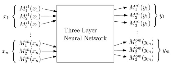
Figure 1.
The architecture of FNN: A normal three-layer neural network that takes the membership values of the input and output variables’ fuzzy numbers as input and output data.
- Step 1: Compute membership values for each training data. Given the set of training data with , they are first converted to membership values , where , , , ⋯, , , , , , , …, , , , based on their corresponding membership functions.
- Step 2: Train a fuzzy neural network. Taking as inputs of the input neurons and as the reference outputs of output neurons, an ANN, consisting of an input layer, a hidden layer and an output layer, is trained using back-propagation algorithm.
Steps 1 and 2 train an FNN. Based on the trained neural, Steps 3–8 describe the process to extract a fuzzy rule based on a representative input pattern .
- Step 3: Compute causal index for each pair of input neurons and output neurons:where , , , and .
- Step 4: Select the output variable. First, compute the relative causal index for each output variable :and the variable with the maximal is selected as the output variable, denoted as .
- Step 5: Select the output fuzzy number for . Compute the relative causal index for each fuzzy number v of :and the fuzzy number with the maximal , denoted as , is the selected fuzzy number.
- Step 6: Transfer negative causal indexes to positive ones. For each input variable , if ,and repeat for and .
- Step 7: Select the input fuzzy number for each input variable. For each input variable , compute the relative causal index related to its fuzzy numbers :and the fuzzy number with the maximal value, say , is determined as the fuzzy number for .
- Step 8: Extract a fuzzy rule. The final generated fuzzy rule is:
2.2. The Algorithm of iDRF-2
iDRF-2 extracts rules from an ANN using (continuous) Boolean functions to approximate the behavior of neurons. The ANN is trained by either discrete variables whose domain of discussion is , or continuous variables whose domain of discussion is the continuous domain . This is because any discrete variable can be transformed to Boolean dummy variables whose values are 0 or 1, and any continuous data can be normalized to The activation function for each neuron is a monotone increasing function whose range is , e.g., the sigmoid function. The main idea to extract rules from such a trained ANN is that the value at each neuron is approximated by a Boolean value, and the relation between its input neurons and itself is described as a Boolean function. For example, as shown in Figure 2, the values of are 0 or 1. There are total combinations, denoted as , in the input space. The Boolean value of the output neuron can be computed based on the following Boolean function:
where
is a real value of the output neuron, which is computed based on the trained neural network, and
with for and for in . The existence condition of each element in (1) based on the trained weights is described in Theorem 1.
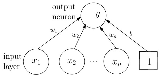
Figure 2.
A single layer perceptron in the trained neural network.
Theorem 1
([14]). For each perceptron in a trained ANN, suppose the activation function S and the trained weights are , …, , b. Let . If , then exists in the approximate Boolean function.
By substituting the Boolean functions of hidden neurons into the output neurons’ Boolean functions, we can obtain the Boolean functions of the output neurons with respect to the input neurons. The method is also extended to continuous variables. Given a real polynomial function , where a and b are real values, . If is a multivariate polynomial function, then . Then, three logical operations are defined: , and . Based on the above definitions, given a perceptron shown in Figure 2, the output neuron can be approximated by a continuous Boolean function: , where with or , and can be determined based on Theorem 1.
We point out that each rule extracted from Reference [14] can be translated to a fuzzy rule, where each linguistic variable in the fuzzy rules has only two fuzzy numbers, and , and the membership functions are and , respectively. For example, if there exists a rule , the corresponding fuzzy rule is:
2.3. The Algorithm of iDRF-3
Focusing on both discrete and continuous data, the authors in Reference [15] proposed a decision tree-based rule extraction from a trained three-layer ANN, i.e., the input layer, a hidden layer, and the output layer. By clustering on the continuous values and generating the boundaries of clusters, a decision tree of each perceptron can be extracted. The detailed process is as follows.
- Step 1: Select a target pattern and set the corresponding output unit. In this step, the continuous domain is discretized into a set of intervals by clustering, each of which is regarded as a pattern.
- Step 2: Build a decision tree to describe the relationship between the target pattern and the activation patterns of hidden neurons. Here, the activation patterns are also generated by clustering on the data computed by the samples. In the tree, the target pattern is the class variable and the activation patterns are attributes. Based on the decision tree, we can extract intermediate rules, simplify the rules, and eliminate redundant rules.
- Step 3: For all hidden neurons, build a decision tree between each hidden neuron and the input neurons. In this tree, the input variables of sample data are the attribute variable, and the discretized patterns generated in Step 2 are the class variables. Similarly, we extract a set of input rules, simplify these rules, and eliminate redundant rules.
- Step 4: Generate the total rules by substituting the input rules for the intermediate rules. Thus, we can generate the total rules, which describe the relationships between the selected output pattern and the input patterns.
- Step 5: Merge the total rules for simplification by integrating continuous ranges with the hill-climbing approach.
- Step 6: For all possible output patterns, repeat Steps 1–5, and we can extract all rules that can approximate the trained ANN.
Similarly, the extracted rules can be translated to a set of fuzzy rules, where the input and output patterns are fuzzy numbers, and their membership functions are determined based on the clustering results. For example, suppose the continuous domain of a continuous variable is , which is divided into three intervals after clustering: , , . We then have three fuzzy numbers, denoted as L, M, and H, and their membership functions are shown in Figure 3.
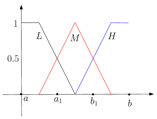
Figure 3.
The membership functions of the fuzzy numbers related to a variable x.
3. Experiment Preparations
This section gives the preparations of the comparison experiments. Specifically, we introduce the sets of training data used in this paper, the neural networks trained by the data sets, and the measure for comparison.
3.1. Training Data Sets
In this paper, we focus on three kinds of data sets: discrete data sets, continuous data sets, and hybrid data sets.
3.1.1. Discrete Training Data
As shown in Table 1, the sets of discrete data are generated from three basic logical operators: , , and , which have been widely used, such as References [14,16,25]. Based on the five discrete data sets, we will train three ANNs to approximate the execution of , , and , respectively.

Table 1.
The sets of discrete training data.
3.1.2. Continuous Training Data
The continuous training data sets are generated from two continuous multi-variable functions:
Here, the input variables are and , and the output variable is y. All of them are continuous domains, and the ranges of input variables are both . The input training data is , where .
3.1.3. Hybrid Training Data
We apply the iris data set as our hybrid training data. In the iris data set, the input variables are four flower features: sepal length, sepal width, petal length, and petal width. They are continuous values and determine the flower types, i.e., Setosa, Versicolor, and Virginica. Hence, the output is the flower type, which is a discrete variable. Figure 4 shows the distribution of the three kinds of flowers with respect to the normalized petal length and petal width. We can find that, with these two features, the flower can almost be classified. Hence, for simplicity, we select these two features as the input neurons of an ANN.
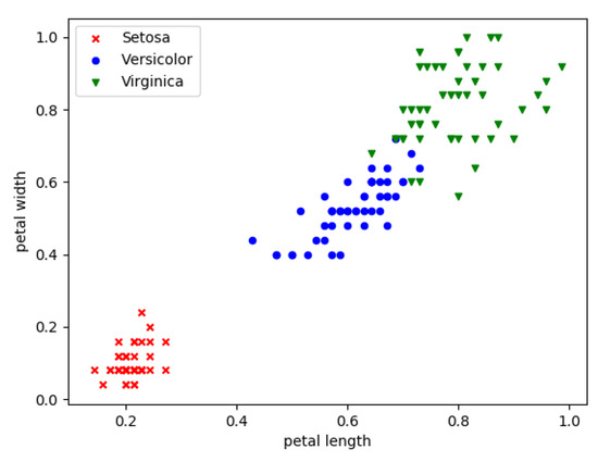
Figure 4.
The relationship between features and types in the iris data set.
3.2. The Architectures of the Trained ANNs
Based on the three kinds of training data sets, we can train an ANN for each data set using the back-propagation algorithm. For the discrete and continuous data sets, we use networks, i.e., 2 input neurons, 4 hidden neurons, and 1 output neuron, while, for the iris data set, a network is applied. Hence, the trained ANNs are shown in Figure 5. The accuracy is 1, 1, 1, 1, 0.932, and 0.967, respectively.
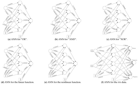
Figure 5.
The trained ANNs for different data sets.
3.3. Similarity Measure among Fuzzy Rules
Given a fuzzy rule benchmark and the set of fuzzy rules extracted from an ANN, we need to evaluate how consistent the two rule sets is. The basic measure is the accuracy of the generated rules, compared with the benchmark, i.e., how many rules are in the benchmark. There may also have rules that are not in the benchmark. We also need to evaluate the inaccuracy of such rules with respect to the benchmark.
There are some measures proposed to describe the relation between two fuzzy numbers [33,34,35]. They usually focus on their membership functions. However, in this paper, we focus on the interpretability of ANNs using fuzzy rules, rather than using fuzzy rules to approximate the original system or as a predictor, so we use an index-based measure, which is a rough but intuitive measure, to describe the difference of two fuzzy numbers related to a variable. The basic idea is that the difference between two fuzzy numbers whose strict 0-cuts are disjoint is larger than the two sets whose strict 0-cuts are overlapped.
Definition 1.
Given a variable x and the set of its fuzzy numbers A, its index function is defined as , where is the set of positive integers.
For example, given the fuzzy numbers shown in Figure 3, we have , , and . Based on the index function, we use the index vector to represent a fuzzy rule.
Definition 2.
Given a fuzzy rule r: “IF is and … and is , THEN is and … and is ”, the index vector of the rule is .
Based on Definition 2, we represent a fuzzy rule by a point in the Euclidean space. Since all the rules describe the same system, the index vector of each rule has the same dimensions. So, we can describe the difference of two rules by the distance of their index vectors and evaluate the difference between a rule and the benchmark.
Definition 3.
Given an extracted rule r and the corresponding rule benchmark , , the difference between r and is . The difference between r and is .
For example, given an extracted rule r:
and a benchmark rule :
where each variable has three fuzzy numbers: small, middle, and large, then their difference is . Clearly, if a rule is in the benchmark set, the difference between the rule and the benchmark is 0. Based on Definition 3, we define the similarity measure of the set of generated rules with respect to its benchmark.
Definition 4.
Given the benchmark set of rules and a set of extracted rules , where and . The inaccuracy of R, denoted as , is defined as .
4. Evaluation on iDRF-1
In this section, we evaluate iDRF-1 on the three data sets. Each variable is fuzzified by three fuzzy numbers: S (small), M (middle), and L (large), whose membership functions are shown in Figure 6, where and .
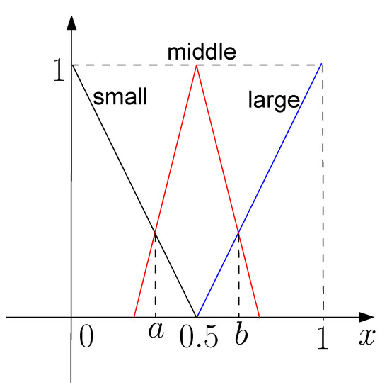
Figure 6.
Fuzzy numbers and their membership functions in iDRF-1.
4.1. Fuzzy Rule Generation Using DFR
Before extracting fuzzy rules via iDRF-1, we first apply DFR [25] to generate the benchmark of fuzzy rules for each data set. In this method, fuzzy rules are generated from data directly. The inputs of the proposed algorithm is the set of training data pairs, each of which contains the values of input and output variables. It contains the following steps.
- Step 1: Fuzzification. This step divides the domain of discussion of the input and output variables into a set of fuzzy regions using triangle membership functions.
- Step 2: Fuzzy rule generation. Each training data will generates a fuzzy rule by assigning each variable with the fuzzy number with the maximal membership value.
- Step 3: Rule simplification. For each rule generated from a data, a degree, which is the product of the membership values and the priori data confidence, is assigned to it. For each group of conflict rules, i.e., the rules with the same IF part but different THEN parts, only the one that has the maximum degree is selected.
- Step 4: Rule base determination. The final rule base consists of the rules generated from data and those from human experts.
Hence, with the same membership functions, we can generate fuzzy rules for each data set. Table 2 and Table 3 give the fuzzy rules for the three discrete data sets and for the two continuous data sets, respectively. The fuzzy rules extracted from the iris data set are:
Table 2.
The benchmark of fuzzy rules for discrete data sets.
Table 3.
The benchmark of fuzzy rules for continuous data sets.
- IF is S and is S, THEN is Setosa;
- IF is M and is M, THEN is Versicolor;
- IF is M and is L, THEN is Virginica;
- IF is L and is M, THEN is Virginica;
- IF is L and is L, THEN is Virginica.
4.2. Rule Extraction from FNNs
In this section, we describe the fuzzy rules extracted from the FNNs. The architecture of each FNN is after fuzzification.
4.2.1. Discrete Data Sets
Table 4 gives the rules for discrete data sets based on iDRF-1. Based on Table 4, we can find that iDRF-1 may generate wrong rules. For example, in the rules for the “OR” operator, the first two rules are consistent with the rules in the benchmark set given in Table 2, while the third rule is wrong. However, even though the second rule is in the benchmark set, it is extracted from the sample pattern “ is small and is large”, i.e., the sample data . It is generated from a wrong data pattern. Moreover, the two consistent rules for “AND” are generated from wrong data patterns, while the three consistent rules for “XOR” are generated from the right data patterns.
Table 4.
Fuzzy rules generated from discrete data sets with iDRF-1.
4.2.2. Continuous Data Sets
Table 5 shows the rules generated for the two continuous data sets with iDRF-1. These rules are generated from nine input data samples, which represent nine data patterns: . Each input data is computed as the mean of the training data with the same data pattern. From Table 5, all the rules generated for the linear function are in the set of benchmark rules given in Table 3, while the second and third rules for the nonlinear function are inconsistent with those in Table 3. Moreover, some input data patterns return wrong rules. For the linear function, the input data pattern (S, M) generates the first rule in Table 5, the input data patterns (M, S) and (M, M) generate the third rule in Table 5, and the patterns (M, L), (L, M) and (L, L) generate the fifth rule in Table 5. For the nonlinear function, the three input patterns, i.e., (M, M), (M, L), and (L, M), generate the right fuzzy rules.
Table 5.
Fuzzy rules generated for continuous data sets.
4.2.3. The iris Data Set
The rules generated for the iris data set is as follows.
- IF is middle and is middle, THEN is Versicolor;
- IF is small and is small, THEN is Setosa;
- IF is large and is large, THEN is Virginica.
Even though the rules generated by iDRF-1 are in the benchmark of fuzzy rules, they are extracted from wrong input data patterns. Actually, the three rules are extracted from the input patterns (small, small), (middle, middle), and (large, large), respectively.
4.3. Analysis and Evaluation on iDRF-1
In this subsection, we give more detailed analysis of iDRF-1 based on the generated rules. Table 6 gives the statistic data of the generated data by iDRF-1 on different data sets. The second column shows the number of extracted rule, and the third and fourth columns show the accuracy and inaccuracy of the generated rules.
Table 6.
Statistic data of the extracted fuzzy rules.
Based on the results, we can find that the generated rules by iDRF-1 are not accurate, and, in most of the data sets, wrong rules are generated. What is worse, iDRF-1 is not robust and not reliable. We need to point out that the rules shown above are only for some trial, and different trials will generate different rules even though the accuracy is almost the same. In the interpretability of ANNs, we do not know the ground truth of fuzzy rules; thus, we have no criteria to select which the best trial to generate fuzzy rules.
In conclusion, iDRF-1 is not suitable to extract fuzzy rules to explain the relationship between input and output data. Hence, iDRF-1 cannot be used as an explanation of ANNs.
5. Evaluation on iDRF-2
In this section, we first generate fuzzy rules using iDRF-2. For comparison, with the membership functions computed from iDRF-2, we generate fuzzy rules based on DFR. Finally, we give an evaluation on iDRF-2.
5.1. (Continuous) Logical Expressions and Fuzzy Rule Generation
As described in Section 2.2, given the trained ANNs shown in Figure 5, each discrete variable is approximated by two values (i.e., 0 or 1), and each continuous variable x is approximated by two functions (i.e., x or 1 − x). Hence, we can obtain the (continuous) logical expressions based on iDRF-2. The results are shown in Table 7, where “” represents “”, "" represents “”, and represents the negative of . Note that, in the continuous logical expression, means , while means .
Table 7.
Rules extracted by DFR and iDRF-2.
Based on the logical expression, we can obtain the related fuzzy rules. Take the logical expression for the nonlinear function as an example. If and , , so we have ; if and , , so we have ; similarly, if and , ; if and , . Hence, we have the following fuzzy rules:
- IF is S and is S, THEN y is S,
- IF is L and is S, THEN y is L,
- IF is S and is L, THEN y is L,
- IF is L and is L, THEN y is S.
Similarly, we can generate fuzzy rules for other data sets.
5.2. Fuzzy Rule Generation Using DFR
Now, we apply DFR to generate fuzzy rules from data directly. Based on the logical expression, we can fuzzify each variable into two fuzzy numbers: S (small) and L (large), whose membership functions are given in Figure 7. Hence, based on DFR, we find that the rules for the discrete data sets are the same as those given in Table 2, and the rules for the linear function are:
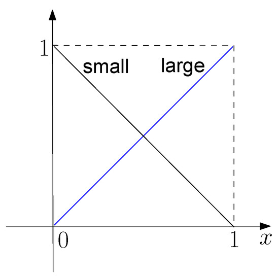
Figure 7.
Membership functions for a variable associated with two fuzzy numbers.
- IF is S and is S, THEN y is S;
- IF is S and is L, THEN y is S;
- IF is L and is S, THEN y is S;
- IF is L and is L, THEN y is L.
The rules for the iris data set are:
- IF is S and is S, THEN y is Setosa;
- IF is S and is L, THEN y is Versicolor;
- IF is L and is S, THEN y is Versicolor;
- IF is L and is L, THEN y is Virginica.
Note that we cannot generate proper rules for the nonlinear function based on DFR since each potential IF part has multiple THEN parts with the same rule degree.
5.3. Analysis and Evaluation on iDRF-2
Table 7 also gives a comparison of the generated rules based on DFR and iDRF-2. In the table, the third column shows the number of rules generated by DFR where each variable is associated with two fuzzy numbers (i.e., S and L), and the fourth column shows the number of rules generated by iDRF-2 where the first and the second items represent the numbers of rules in and not in the set of rules generated by DFR, respectively. We can find that except for the nonlinear function, with 2-fuzzy-number fuzzification, the accuracy of iDRF-2 is 100%, and inaccuracy is 0, which means the rules generated by iDRF-2 are the same as those generated by DFR. Hence, iDRF-2 performs well if each variable is fuzzified with two fuzzy numbers.
However, the main limitation of iDRF-2 is that it can only deal with the situation that each variable can be fuzzified with two fuzzy numbers directly or after some transformation. Hence, iDRF-2 can be used and perform well for data with discrete domains since the discrete domains can be reduced to domain by dummy variables, which can be well fuzzified with two fuzzy numbers. For the continuous domains, if a variable is fuzzified with only two fuzzy numbers, it may induce large errors or inaccuracy. For example, Figure 8 shows the data distribution of the linear function data set, where the points show the distribution of the fuzzy numbers of y with respect to the input variables, and the alphabets show the output fuzzy numbers of the generated rules with respect to the combinations of the input fuzzy numbers. For the 2-fuzzy-number fuzzification, there are 25% data whose relationship between the input and output variables cannot be represented by the generated rules (Figure 8a), while, for 3-fuzzy-number fuzzification, 22% data cannot be described correctly by the generated rules (Figure 8b). Using DFR, we can get higher accuracy with more fuzzy numbers, which cannot be achieved by iDRF-2.
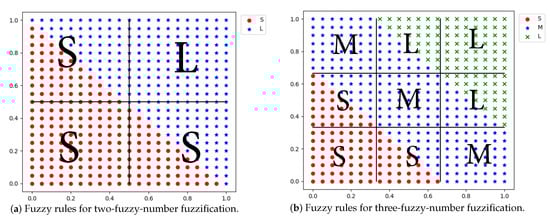
Figure 8.
Data distributions and generated fuzzy rules on the linear function data set.
In conclusion, iDRF-2 can generate accurate fuzzy rules to describe the relation of discrete data sets but does not perform well in continuous and hybrid data sets. Hence, it can be used to explain ANNs which are applied in discrete domains but is not suitable to explain ANNs trained in continuous domains.
6. Evaluation on iDRF-3
In this section, we evaluate the performance of iDRF-3.
6.1. Clustering and Fuzzy Rule Generation
Based on iDRF-3, we first generate the hidden-output and input-hidden decision trees. To generate the hidden-output decision tree, we need to compute the values of the hidden neurons based on the training data. In the sequel, we give the detailed procedure for each data set.
6.1.1. Discrete Data Sets
Given the training data and the well-trained ANNs, we can compute the values of the four hidden neurons, denoted as . Based on the data set , we can build the decision tree for the hidden-output layer. Take the “XOR” data set as an example, whose trained ANN is shown in Figure 5c, and the values of the input, hidden, and output neurons are shown in Table 8.
Table 8.
The values of input, hidden, and output neurons for the “XOR” data set.
Based on the hidden and output data, we can build a hidden-output decision tree for each target output. Figure 9a shows the hidden-output decision tree for the target . Based on the decision tree, we have an intermediate rule: . Then, we can build the input-hidden decision tree with the target , which is shown in Figure 9b. Based on this decision tree, we have and . Hence, we can extract the following rules for the target : “IF and , THEN ” and “IF and , THEN ”. Similarly, for the target , the decision trees are shown in Figure 10, and we can obtain the rules: “IF and , THEN ” and “IF and , THEN ”. For the data sets of “AND” and “OR”, we can do the same procedure and generate the rules.
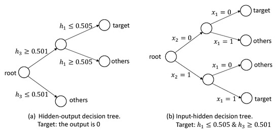
Figure 9.
The hidden-output decision tree for the target in the “XOR” data set.
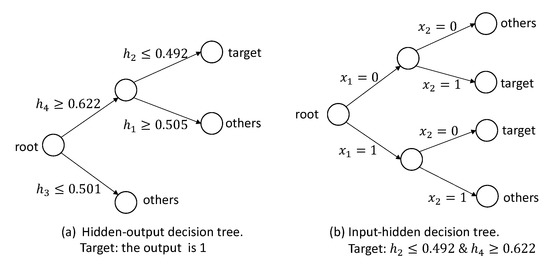
Figure 10.
The hidden-output decision tree for the target in the “XOR” data set.
6.1.2. Continuous Data Sets
For the continuous data sets, we first use k-mean to cluster the output values into three categories. For each category, we then build the related hidden-output and input-hidden decision trees. For example, in the data set of the linear function, the output is clustered into three discrete ranges: , , and . Figure 11a shows the decision tree whose target is that the output is in the first discrete range, and we can extract a rule “IF & →”. Figure 11b represents the input-hidden tree with the target & , where each rectangle represents a path in the tree that leads to the target leaf, and the number in it denotes the number of samples belonging to this path. For example, the largest rectangle represents the path “ & → & ”, and there are 64 samples satisfying this path. For simplicity and to reduce over-fitting, this decision tree is then pruned by omitting the rectangles with a few samples and approximating some adjacent rectangles with one rectangle. Hence, the decision tree in Figure 11b is pruned to three rectangles, i.e., the three large blue rectangles, which can extract three rules: “ & → target”, “ & → target”, and “ & → target”. Finally, we can generate the following input-output rules:
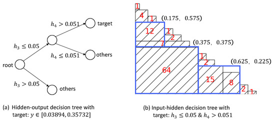
Figure 11.
Decision trees for the target .
- & →;
- & →;
- & →.
Similarly, the decision trees for the range is shown in Figure 12. We can extract the following rules:
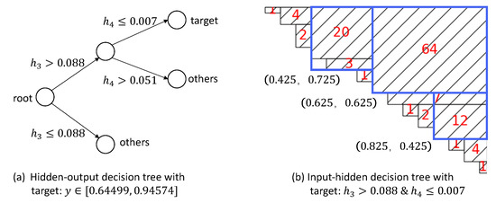
Figure 12.
Decision trees for the target .
- & →;
- & →;
- & →.
Figure 13 shows the decision trees for the middle range. For the input-hidden tree, it is hard to find proper pruning directly. However, based on the results of the other two ranges, we can find that we can partition each input variable into , , and . Based on such a partition, as shown in Figure 13b, we can obtain the following rules:
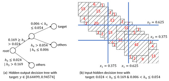
Figure 13.
Decision trees for the target .
- & →;
- & →;
- & →.
6.1.3. iris Data Set
In the iris data set, the output variable is discrete, so we can build decision trees for each discrete value. First, for the type “Setosa”, the decision trees are shown in Figure 14. Based on the decision trees, we can extract the following rule: . Second, for the type “Versicolor”, the pruned decision trees are shown in Figure 15, and we can extract a rule: . Based on the decision trees, shown in Figure 16, for the target Virginica, we can extract rules: , and .
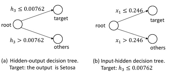
Figure 14.
The decision trees for the target Setosa.
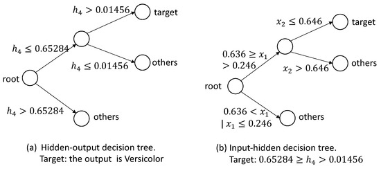
Figure 15.
The decision trees for the target Versicolor.
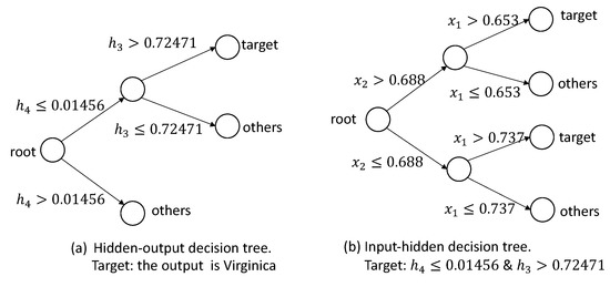
Figure 16.
The decision trees for the target Virginica.
Based on these rules, we fuzzify either input variable into S, M, and L, whose membership functions are shown in Figure 6 with and , and generate fuzzy rules:
- IF is S, THEN y is Setosa;
- IF is M and is S, THEN y is Versicolor;
- IF is M and is M, THEN y is Versicolor;
- IF is L, THEN y is Virginica.
6.2. Fuzzy Rule Generation Using DFR
For the discrete data sets, no matter what kinds of membership functions applied, the generated fuzzy rules using iDRF-3 are the same as those generated with DFR, consisting of those given in Table 2. For the continuous data sets, if the membership functions are determined with the results of data clustering, then the fuzzy rules generated by DFR and iDRF-3 are the same, which have the same formula with those in Table 3. Based on the new membership functions, we can obtain the fuzzy rules for the iris data set using DFR, which is shown as follows.
- IF is S and is S, THEN y is Setosa;
- IF is M and is M, THEN y is Versicolor;
- IF is M and is L, THEN y is Virginica;
- IF is L and is M, THEN y is Virginica;
- IF is L and is L, THEN y is Virginica.
6.3. Analysis and Evaluation of iDRF-3
Based on the generated fuzzy rules from DFR and iDRF-3, the discrete and continuous data sets, DFR and iDRF-3 are consistent. For the hybrid data set, comparing the two sets of fuzzy rules by DFR and iDRF-3, we can find that, in the set of fuzzy rules generated by iDRF-3, there are four rules that DFR does not generate: “IF is S and is M, THEN y is Setosa”, “IF is S and is L, THEN y is Setosa”, “IF is M and is S, THEN y is Versicolor”, and “IF is L and is S, THEN y is Virginica”, while the rule “IF is L and is M, THEN y is Virginica” does not exist in the rules generated by iDRF-3.
The reason for the missing of the four rules using DFR is that there is no data related to these four rules, which means that their degrees are 0, so DFR does not generate these rules, while iDRF-3 focuses on the boundaries that can separate different kinds of data without considering the region without any data. This means the extracted rules may contain empty regions using the generated boundary. Moreover, to reduce over-fitting, we prune some branches of the decision trees since there are a few samples in the leaf nodes with large depth. This will result in the missing of some fuzzy rules generated by DFR since they only contain very few samples. However, one drawback of iDRF-3 is that, sometimes, it is not easy to extract proper rules from the decision trees and compute a unified membership function for a variable among different output targets, especially for data with poor separability.
In conclusion, both DFR and iDRF-3 can generate proper fuzzy rules for discrete, continuous, and hybrid data sets, but may induce errors. Hence, iDRF-3 can be applied to explain ANNs trained by discrete, continuous, and hybrid data sets, and cannot guarantee the accuracy if we have no knowledge of the data relations (e.g., separability).
7. Conclusions
In this paper, we evaluate the performance of three widely-used methods to explain ANNs with fuzzy rules. The results show that the method based on causal index cannot explain ANNs, while the method based on Boolean logical expression can be used to explain ANNs trained by discrete data sets, and the method based on decision trees can be used to explain ANNs on all data sets but cannot guarantee the accuracy for data with poor separability. We find that, even though some methods have been proposed to extract fuzzy rules from ANNs trained by specific data sets, there is no general method to extract fuzzy rules from ANNs trained by different data sets. Users must carefully select proper methods for rule extraction based on the applications. It is necessary to develop new extraction methods to explain general ANNs in terms of fuzzy rules.
In the future, we will evaluate the three methods on more data sets and investigate other methods for the fuzzy rule-based explanation of ANNs. Since each method has its own limitations, we need to investigate novel methods to explain ANNs using fuzzy rules. Finally, we will also focus on the explanation of deep neural networks.
Author Contributions
Data curation, X.T.; Formal analysis, X.T. and Y.Z.; Investigation, X.T. and Y.Z.; Methodology, Y.Z. and Z.D.; Project administration, Z.D. and Y.L.; Supervision, Z.D.; Writing—original draft, Y.Z.; Writing—review and editing, Z.D. and Y.L. All authors have read and agreed to the published version of the manuscript.
Funding
This research was supported by National Nature Science Foundation of China (Grant Nos.61751210).
Institutional Review Board Statement
Not applicable.
Informed Consent Statement
Not applicable.
Data Availability Statement
Not applicable.
Conflicts of Interest
The authors declare no conflict of interest.
References
- Schütt, K.T.; Arbabzadah, F.; Chmiela, S.; Müller, K.R.; Tkatchenko, A. Quantum-chemical insights from deep tensor neural networks. Nat. Commun. 2017, 8, 1–8. [Google Scholar] [CrossRef]
- Shang, M.; Luo, X.; Liu, Z.; Chen, J.; Yuan, Y.; Zhou, M. Randomized latent factor model for high-dimensional and sparse matrices from industrial applications. IEEE/CAA J. Autom. Sin. 2018, 6, 131–141. [Google Scholar] [CrossRef]
- Liu, L.; Liu, Y.J.; Tong, S. Neural networks-based adaptive finite-time fault-tolerant control for a class of strict-feedback switched nonlinear systems. IEEE Trans. Cybern. 2018, 49, 2536–2545. [Google Scholar] [CrossRef]
- Zhou, H.; Zhao, H.; Zhang, Y. Nonlinear system modeling using self-organizing fuzzy neural networks for industrial applications. Appl. Intell. 2020, 50, 1657–1672. [Google Scholar] [CrossRef]
- El Hamidi, K.; Mjahed, M.; El Kari, A.; Ayad, H. Adaptive control using neural networks and approximate models for nonlinear dynamic systems. Model. Simul. Eng. 2020, 2020, 8642915. [Google Scholar]
- Amisha, P.M.; Pathania, M.; Rathaur, V.K. Overview of artificial intelligence in medicine. J. Fam. Med. Prim. Care 2019, 8, 2328–2331. [Google Scholar] [CrossRef]
- Ding, Z.; Zhou, Y.; Zhou, M. Modeling self-adaptive software systems with learning Petri nets. IEEE Trans. Syst. Man Cybern. Syst. 2015, 46, 483–498. [Google Scholar] [CrossRef]
- Samek, W.; Montavon, G.; Lapuschkin, S.; Anders, C.J.; Müller, K.R. Explaining deep neural networks and beyond: A review of methods and applications. Proc. IEEE 2021, 109, 247–278. [Google Scholar] [CrossRef]
- Holzinger, A. From machine learning to explainable AI. In Proceedings of the 2018 World Symposium On Digital Intelligence For Systems And Machines (DISA), Košice, Slovakia, 23–25 August 2018; pp. 55–66. [Google Scholar]
- Bau, D.; Zhu, J.Y.; Strobelt, H.; Lapedriza, A.; Zhou, B.; Torralba, A. Understanding the role of individual units in a deep neural network. Proc. Natl. Acad. Sci. USA 2020, 117, 30071–30078. [Google Scholar] [CrossRef]
- Craven, M.W. Extracting Comprehensible Models from Trained Neural Networks. Ph.D. Thesis, Department of Computer Sciences, University of Wisconsin-Madison, Madison, WI, USA, 1996. [Google Scholar]
- Ding, Z.; Zhou, Y.; Zhou, M. Modeling self-adaptive software systems by fuzzy rules and Petri nets. IEEE Trans. Fuzzy Syst. 2017, 26, 967–984. [Google Scholar] [CrossRef]
- Hailesilassie, T. Rule extraction algorithm for deep neural networks: A review. Int. J. Comput. Sci. Inf. Secur. 2016, 14, 376–381. [Google Scholar]
- Tsukimoto, H. Extracting rules from trained neural networks. IEEE Trans. Neural Netw. 2000, 11, 377–389. [Google Scholar] [CrossRef] [PubMed]
- Sato, M.; Tsukimoto, H. Rule extraction from neural networks via decision tree induction. In Proceedings of the International Joint Conference on Neural Networks, Washington, DC, USA, 15–19 July 2001; Volume 3, pp. 1870–1875. [Google Scholar]
- Fu, L. Rule generation from neural networks. IEEE Trans. Syst. Man Cybern. 1994, 24, 1114–1124. [Google Scholar]
- Taha, I.A.; Ghosh, J. Symbolic interpretation of artificial neural networks. IEEE Trans. Knowl. Data Eng. 1999, 11, 448–463. [Google Scholar] [CrossRef]
- Hayashi, Y.; Sato, R.; Mitra, S. A new approach to three ensemble neural network rule extraction using recursive-rule extraction algorithm. In Proceedings of the 2013 International Joint Conference on Neural Networks (IJCNN), Dallas, TX, USA, 4–9 August 2013; pp. 1–7. [Google Scholar]
- Zilke, J.R.; Mencía, E.L.; Janssen, F. Deepred–rule extraction from deep neural networks. In Proceedings of the International Conference on Discovery Science, Bari, Italy, 19–21 October 2016; pp. 457–473. [Google Scholar]
- Bologna, G.; Hayashi, Y. A rule extraction study on a neural network trained by deep learning. In Proceedings of the 2016 International Joint Conference on Neural Networks (IJCNN), Vancouver, BC, Canada, 24–29 July 2016; pp. 668–675. [Google Scholar]
- Lo, J.-C.; Yang, C.-H. A heuristic error-feedback learning algorithm for fuzzy modeling. IEEE Trans. Syst. Man Cybern. Part A Syst. Hum. 1999, 29, 686–691. [Google Scholar]
- Benítez, J.M.; Castro, J.L.; Requena, I. Are artificial neural networks black boxes? IEEE Trans. Neural Netw. 1997, 8, 1156–1164. [Google Scholar] [CrossRef]
- Castro, J.L.; Mantas, C.J.; Benítez, J.M. Interpretation of artificial neural networks by means of fuzzy rules. IEEE Trans. Neural Netw. 2002, 13, 101–116. [Google Scholar] [CrossRef]
- Fahmy, R.; Zaher, H. A comparison between fuzzy inference systems for prediction (with application to prices of fund in Egypt). Int. J. Comput. Appl. 2015, 109, 6–11. [Google Scholar] [CrossRef]
- Wang, L.; Mendel, J.M. Generating fuzzy rules by learning from examples. IEEE Trans. Syst. Man Cybern. 1992, 22, 1414–1427. [Google Scholar] [CrossRef]
- Guillaume, S. Designing fuzzy inference systems from data: An interpretability-oriented review. IEEE Trans. Fuzzy Syst. 2001, 9, 426–443. [Google Scholar] [CrossRef]
- Duţu, L.C.; Mauris, G.; Bolon, P. A fast and accurate rule-base generation method for Mamdani fuzzy systems. IEEE Trans. Fuzzy Syst. 2018, 26, 715–733. [Google Scholar] [CrossRef]
- Kim, D. An implementation of fuzzy logic controller on the reconfigurable FPGA system. IEEE Trans. Ind. Electron. 2000, 47, 703–715. [Google Scholar]
- Tzou, Y.-Y.; Lin, S.-Y. Fuzzy-tuning current-vector control of a three-phase PWM inverter for high-performance AC drives. IEEE Trans. Ind. Electron. 1998, 45, 782–791. [Google Scholar] [CrossRef]
- Enbutsu, I.; Baba, K.; Hara, N. Fuzzy rule extraction from a multilayered neural network. In Proceedings of the International Joint Conference on Neural Networks (IJCNN), Seattle, WA, USA, 8–12 July 1991; Volume 2, pp. 461–465. [Google Scholar]
- Wu, S.; Er, M.J.; Gao, Y. A fast approach for automatic generation of fuzzy rules by generalized dynamic fuzzy neural networks. IEEE Trans. Fuzzy Syst. 2001, 9, 578–594. [Google Scholar]
- Leng, G.; McGinnity, T.M.; Prasad, G. An approach for on-line extraction of fuzzy rules using a self-organising fuzzy neural network. Fuzzy Sets Syst. 2005, 150, 211–243. [Google Scholar] [CrossRef]
- Setnes, M.; Babuska, R.; Kaymak, U.; van Nauta Lemke, H.R. Similarity measures in fuzzy rule base simplification. IEEE Trans. Syst. Man Cybern. Part B (Cybern.) 1998, 28, 376–386. [Google Scholar] [CrossRef]
- Johanyák, Z.C.; Kovács, S. Distance based similarity measures of fuzzy sets. In Proceedings of the 3rd Slovakian-Hungarian Joint Symposium on Applied Machine Intelligence, Herl’any, Slovakia, 21–22 January 2005; Volume 2005. [Google Scholar]
- McCulloch, J.; Wagner, C.; Aickelin, U. Measuring the directional distance between fuzzy sets. In Proceedings of the 2013 13th UK Workshop on Computational Intelligence (UKCI), Guildford, UK, 9–11 September 2013; pp. 38–45. [Google Scholar]
Publisher’s Note: MDPI stays neutral with regard to jurisdictional claims in published maps and institutional affiliations. |
© 2021 by the authors. Licensee MDPI, Basel, Switzerland. This article is an open access article distributed under the terms and conditions of the Creative Commons Attribution (CC BY) license (https://creativecommons.org/licenses/by/4.0/).