Delay Stability of n-Firm Cournot Oligopolies

Abstract

The dynamic behavior of n-firm oligopolies is examined without product differentiation and with linear price and cost functions. Continuous time scales are assumed with best response dynamics, in which case the equilibrium is asymptotically stable without delays. The firms are assumed to face both implementation and information delays. If the delays are equal, then the model is a single delay case, and the equilibrium is oscillatory stable if the delay is small, at the threshold stability is lost by Hopf bifurcation with cyclic behavior, and for larger delays, the trajectories show expanding cycles. In the case of the non-equal delays, the stability switching curves are constructed and the directions of stability switches are determined. In the case of growth rate dynamics, the local behavior of the trajectories is similar to that of the best response dynamics. Simulation studies verify and illustrate the theoretical findings.

1. Introduction

Examining oligopoly models is a very frequently studied research area in mathematical economics. Based on the pioneering work of Cournot [1], many researchers were devoted to this interesting and challenging model and its variants and extensions. One frequently studied extension is obtained by considering the dynamic behavior of the firms. These models can be divided into several categories including linear and nonlinear models, discrete and continuous time scales, best response, and gradient adjustments. For discrete time scales Theocharis [2] showed that the equilibrium of n-firm linear oligopolies without product differentiation is asymptotically stable if $n=2$, marginally stable if $n=3$ and unstable if $n>3$. For continuous time scales, McManus and Quandt [3] showed that the equilibrium is always asymptotically stable in the linear case regardless of the values of the positive speeds of adjustments. These classical results already indicated that the dynamic properties of the equilibrium strongly depends on the selection of time scales. Several generalizations and extensions were then introduced and studied in the literature. The early results up to the mid-70s are summarized in Okuguchi [4] and their multiproduct generalizations are presented in Okuguchi and Szidarovszky [5]. Different aspects of the classical Theocharis model were then examined by several authors including Canovas et al. [6], Hommes et al. [7], Lampart [8], Puu [9,10], Matsumoto and Szidarovszky [11] among others. Nonlinear models are discussed in Bischi et al. [12] and their extensions including delays are examined in Matsumoto and Szidarovszky [13].

In this paper, we reconsider the classical Theocharis model by examining the dynamic behavior of linear n-firm oligopolies without product differentiation and with the additional assumption that the firms face both implementation and information delays. As it is well known that in the linear case best response and gradient adjustment processes are equivalent with different speeds of adjustments, we deal only with best response dynamics. It is assumed that the firms face equal delays in both types. If the implementation and information delays are equal, then the model is equivalent with a single delay case mathematically. In this case, we show that the equilibrium is oscillatory asymptotically stable if the common delay is sufficiently small, at the threshold Hopf bifurcation occurs with cyclic and for larger delays expanding cyclic trajectories. If the delays are different, then a two-delay model is obtained. The stability switching curves are first constructed and then the directions of stability switches are determined. Growth rate dynamics result in nonlinear systems, their local linearizations around the equilibrium result in linear dynamics, that is equivalent to the best response case. So the local dynamics of the two systems are equivalent. Simulation studies verify and illustrate the theoretical findings of the paper. Even in the very special case of linear models, our analysis discovered several aspects of the dynamics which were not studied in the literature before. The importance of examining linear models is verified in addition to the fact that linearized nonlinear models have the same mathematical structures.

This paper develops as follows. Section 3 introduces the best response dynamics. First stability switching curves are constructed and then the case of equal delays is discussed in detail. Growth rate dynamics are introduced in Section 4. First, the stability switching curves are shown and then the directions of stability switches are determined. In both sections, numerical results and simulation studies verify and illustrate the theoretical results. Section 5 offers conclusions and outlines further research directions.

2. Model

The classical oligopoly model is presented reconsidering the classical results of Theocharis [2] and McManus and Quandt [3]. In the model, n firms are producing a homogeneous output. The price function is assumed to be linear,

$$p=a-b\sum _{j=1}^n{x}_j$$

where $a>0$ is the maximum price, $b>0$ is the slope of the price function and $x_j$ is firm j’s output. The production cost is also assumed to be linear with no fixed cost. The marginal cost of firm j is denoted by $c_j,$ being positive. The profit function of firm $i$ is defined by

$${\pi }_i=\left(a-b\sum _{j=1}^n{x}_j\right)x_i-c_i{x}_i.$$

Under the Cournot competition, the firms decide how much to produce. As we focus only on interior solutions (If the optimal output level of a firm is zero, then the firm leaves the industry, so we can igonore such firms), the first-order condition of firm i for profit maximization is

$$\frac{\partial {\pi }_i}{\partial x_i}=a-2b{x}_i-b\sum _{j\ne i}^n{x}_j-c_i=0$$

and the second-order condition is satisfied,

$$\frac{{\partial }^2{\pi }_i}{\partial x_i^2}=-2b<0.$$

The best reply function is obtained through the first-order condition and depends on the choices of other firms,

$$x_i^{*}=\frac{a-c_i-b{\sum }_{j\ne i}^n{x}_j}{2b}.$$

Let us introduce a new notation,

$${\alpha }_i=\frac{a-c_i}{2b},\beta =\frac{1}{2}\mathrm{and}Q=\sum _{j=1}^n{x}_j$$

and make the conventional assumption:

Assumption 1.

$c_i=c$ for all $i$ and $a>c$.

Assumption 1 implies ${\alpha }_i=\alpha >0$ for all i. As each firm makes an optimal choice at the Cournot equilibrium, its best reply function is written as

$$x_i^{*}=\frac{\alpha -\beta Q^{*}}{1-\beta }.$$

The aggregate output of all firms is obtained by adding the individual outputs,

$$Q^{*}=\sum _{i=1}^n{x}_i^{*}=n\frac{\alpha -\beta Q^{*}}{1-\beta }$$

that is solved for $Q^{*}$ to have

$$Q^{*}=\frac{n\alpha }{1+\left(n-1\right)\beta }.$$

Substituting $Q^{*}$ into the best reply gives the individual output values at the Cournot equilibrium,

$$x_i^e=\frac{\alpha }{1+\left(n-1\right)\beta }\mathrm{for}i=1,2,\dots ,n.$$

3. Best Reply Dynamics

Dynamic interpretation of the oligopoly model depends on how to define a learning process on how each firm observes its competitors’ choices. Theocharis (1960) constructs the best reply dynamics with naive expectations in discrete time scales,

$$x_i(t+1)=\alpha -\beta \sum _{j\ne i}^n{x}_j\left(t\right)$$

where the adjustment to the optimal output in each period is perfect. His provocative result shows that the stability of the Cournot equilibrium is determined only by the number of the firms in an industry as mentioned in the Introduction. McManus and Quandt (1961) makes two reasonable modifications of Theocharis’ assumptions: the discrete-time scales are replaced with continuous-time scales and the imperfect adjustment assumption is adopted in which the direction of output change is proportional to the discrepancy between the optimal and actual values,

$${\dot{x}}_i\left(t\right)=k_i\left[\alpha -\beta \sum _{j\ne i}^n{x}_j\left(t\right)-x_i\left(t\right)\right]\mathrm{with}{k}_i>0.$$

It is demonstrated that the Cournot equilibrium is always stable when the adjustment speeds are the same (i.e., $k_i=k$). Their result is in sharp contrast to Theocharis’ result. We also note that this result remains true if all adjustment speeds are positive.

3.1. Stability Switching

In this study, we move one step forward from the McManus and Quandt model and introduce implementation delays (i.e., ${\tau }_1>0$) on the firm’s own production and information delays (${\tau }_2>0$) on the competitors’ productions,

$${\dot{x}}_i\left(t\right)=k\left[\alpha -\beta \sum _{j\ne i}^n{x}_j(t-{\tau }_2)-x_i(t-{\tau }_1)\right]\mathrm{for}i=1,2,\dots ,n.$$

(1)

Notice that dynamic system (1) has the Cournot equilibrium as the steady-state and its homogeneous part is

$${\dot{x}}_i\left(t\right)=k\left[-x_i(t-{\tau }_1)-\beta \sum _{j\ne i}^n{x}_j(t-{\tau }_2)\right]\mathrm{for}i=1,2,\dots ,n.$$

(2)

The characteristic equation is

$$\phi \left(\lambda \right)=\left(\begin{array}{cccc}\lambda +k{e}^{-\lambda {\tau }_1}& k\beta e^{-\lambda {\tau }_2}& \cdots & k\beta e^{-\lambda {\tau }_2}\\ k\beta e^{-\lambda {\tau }_2}& \lambda +k{e}^{-\lambda {\tau }_1}& \cdots & k\beta e^{-\lambda {\tau }_2}\\ ·& ·& \cdots & \cdots \\ k\beta e^{-\lambda {\tau }_2}& k\beta e^{-\lambda {\tau }_2}& \cdots & \lambda +k{e}^{-\lambda {\tau }_1}\end{array}\right)=0.$$

With new notation,

$$\mathit{D}=diag{\left(\lambda +k{e}^{-\lambda {\tau }_1}-k\beta e^{-\lambda {\tau }_2},\dots ,\lambda +k{e}^{-\lambda {\tau }_1}-k\beta e^{-\lambda {\tau }_2}\right)}_{(n,n)}$$

$$\mathit{a}={\left(k\beta e^{-\lambda {\tau }_2}\right)}_{(n,1)}\mathrm{and}\mathit{b}={\left(1\right)}_{(n,1)},$$

the characteristic equation can be written as

$$\begin{array}{ccc}\hfill \phi \left(\lambda \right)& =& det\left(\mathit{D}+{\mathit{ab}}^T\right),\hfill \\ & =& det\mathit{D}det\left(\mathit{I}+{\mathit{D}}^{-1}{\mathit{ab}}^T\right),\hfill \\ & =& det\mathit{D}\left[1+{\mathit{b}}^T{\mathit{D}}^{-1}\mathit{a}\right].\hfill \end{array}$$

Hence

$$\begin{array}{ccc}\hfill \phi \left(\lambda \right)& =& {\left[\lambda +k{e}^{-\lambda {\tau }_1}-k\beta e^{-\lambda {\tau }_2}\right]}^n\left[1+\frac{nk\beta e^{-\lambda {\tau }_2}}{\lambda +k{e}^{-\lambda {\tau }_1}-k\beta e^{-\lambda {\tau }_2}}\right]\hfill \\ & =& {\left(\lambda +k{e}^{-\lambda {\tau }_1}-k\beta e^{-\lambda {\tau }_2}\right)}^{n-1}\left(\lambda +k{e}^{-\lambda {\tau }_1}+k\beta (n-1)e^{-\lambda {\tau }_2}\right).\hfill \end{array}$$

It follows that we have two possibilities to solve $\phi \left(\lambda \right)=0$,

$$\begin{array}{c}\left(\mathrm{i}\right)\lambda +k{e}^{-\lambda {\tau }_1}-k\beta e^{-\lambda {\tau }_2}=0,\\ \left(\mathrm{ii}\right)\lambda +k{e}^{-\lambda {\tau }_1}+k\beta (n-1)e^{-\lambda {\tau }_2}=0.\end{array}$$

Without delays ${\tau }_1={\tau }_2=0,$ the eigenvalues are negative,

$${\lambda }_1=-k(1-\beta )<0\mathrm{and}{\lambda }_2=-k\left[1+\beta (n-1)\right]<0,$$

implying that the equilibrium is asymptotically stable.

For positive delays, we follow the method discussed in Matsumoto and Szidarovszky [13] based on Gu et al. [14]. Consider equation (i) first. As $\lambda =0$ does not solve equation (i), it can be rewritten as

$$1+a_1\left(\lambda \right)e^{-\lambda {\tau }_1}+a_2\left(\lambda \right)e^{-\lambda {\tau }_2}=0$$

(3)

where

$$a_1\left(\lambda \right)=\frac{k}{\lambda }\mathrm{and}{a}_2\left(\lambda \right)=-\frac{k\beta }{\lambda }.$$

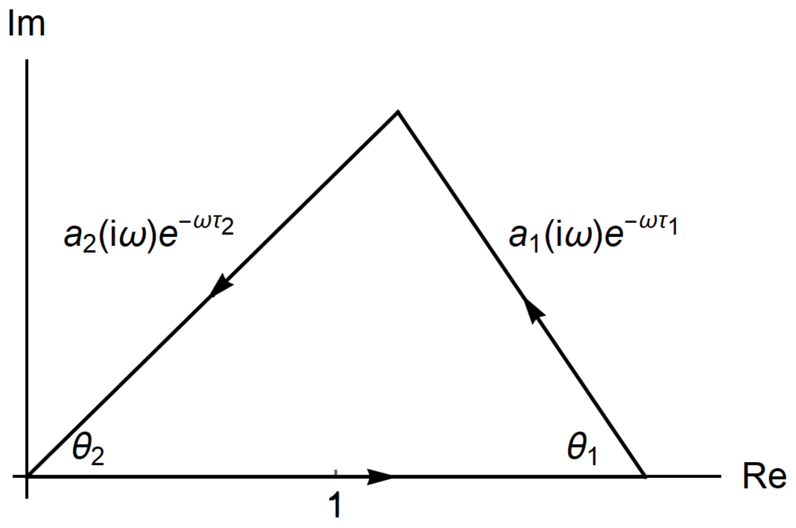
Equation (3) must have a pair of pure imaginary solutions when a stability switch occurs. Hence let $\lambda =i\omega$ with $\omega >0$ (It is possible to take its conjugate with $\omega <0$. Even so, we can arrive at the same result.) and we may consider the three terms in (3) as three vectors in the complex plane with the magnitudes $1,\left|a_1\left(i\omega \right)\right|$ and $\left|a_2\left(i\omega \right)\right|$, respectively. Equation (3) means that if we put these vectors head to tail, they form a triangle with the internal angles ${\theta }_1$ and ${\theta }_2$ as illustrated in Figure 1.

Figure 1. Triangle conditions.

These vectors form a triangle if and only if the sum of the lengths of any two adjacent line segments is not shorter than the length of the remaining line segment:

$$\left|a_1\left(i\omega \right)\right|+\left|a_2\left(i\omega \right)\right|\ge 1$$

and

$$-1\le \left|a_1\left(i\omega \right)\right|-\left|a_2\left(i\omega \right)\right|\le 1.$$

For $\lambda =i\omega ,$

$$a_1\left(i\omega \right)=-i\frac{k}{\omega }\mathrm{and}{a}_2\left(\lambda \right)=i\frac{k\beta }{\omega }$$

where the absolute values are

$$\left|a_1\left(i\omega \right)\right|=\frac{k}{\omega }\mathrm{and}\left|a_2\left(i\omega \right)\right|=\frac{k\beta }{\omega }$$

and the arguments are

$$arg\left[a_1\left(i\omega \right)\right]=\frac{3\pi }{2}\mathrm{and}arg\left[a_2\left(i\omega \right)\right]=\frac{\pi }{2}.$$

From the triangle conditions, we have the interval of $\omega$ for which $\lambda =i\omega$ can be a solution of equation (i) for some ${\tau }_1$ and ${\tau }_2$,

$$\omega \in I=\left[\frac{1}{2}k,\frac{3}{2}k\right].$$

The internal angles of ${\theta }_1$ and ${\theta }_2$ are calculated by the law of cosine as

$${\theta }_1\left(\omega \right)={cos}^{-1}\left[\frac{4{\omega }^2+3k^2}{8k\omega }\right]$$

and

$${\theta }_2\left(\omega \right)={cos}^{-1}\left[\frac{4{\omega }^2-3k^2}{4k\omega }\right].$$

For any $\omega \in I,$ we may find all pairs of $({\tau }_1,{\tau }_2)$ satisfying (3) as follows:

$${\tau }_1^{\pm }(\omega ,{\ell }_1)=\frac{1}{\omega }\left[\frac{3}{2}\pi +\left(2{\ell }_1-1\right)\pi \pm {\theta }_1\left(\omega \right)\right]$$

(4)

and

$${\tau }_2^{\mp }(\omega ,{\ell }_2)=\frac{1}{\omega }\left[\frac{1}{2}\pi +\left(2{\ell }_2-1\right)\pi \mp {\theta }_2\left(\omega \right)\right].$$

(5)

Since a symmetric triangle can be formed below the horizontal axis in Figure 1, four inner angles are defined, $\pm {\theta }_1\left(\omega \right)$ and $\mp {\theta }_2\left(\omega \right)$(double-sign correspondence). By the definitions of the interior angles, we have the followings:

$$arg\left(a_1\left(\omega \right)e^{-i\omega {\tau }_1}\right)+2{\ell }_1\pi \pm {\theta }_1\left(\omega \right)=\pi$$

and

$$arg\left(a_2\left(\omega \right)e^{-i\omega {\tau }_2}\right)+2{\ell }_2\pi \mp {\theta }_2\left(\omega \right)=\pi$$

for ${\ell }_1=0,1,2,\dots$ and ${\ell }_2=0,1,2,\dots$ Solving these equations for ${\tau }_1$ and ${\tau }_2$ yields (4) and (5). So we have two sets of line segments,

$$C_1^{+}({\ell }_1,{\ell }_2)=\left\{\left.({\tau }_1^{+}(\omega ,{\ell }_1),{\tau }_2^{-}(\omega ,{\ell }_2))\right|\omega \in I,\left({\ell }_1,{\ell }_2\right)\in \mathit{Z}\right\}$$

and

$$C_1^{-}({\ell }_1,{\ell }_2)=\left\{\left.({\tau }_1^{-}(\omega ,{\ell }_1),{\tau }_2^{+}(\omega ,{\ell }_2))\right|\omega \in I,\left({\ell }_1,{\ell }_2\right)\in \mathit{Z}\right\}.$$

As ${\ell }_1$ is the horizontal shift parameter and ${\ell }_2$ is the vertical shift parameter, changing these values shifts these segments accordingly. Connecting these segments creates the stability switching curve (SSC, henceforth) under equation (i).

We now turn attention to equation (ii) that can be written as

$$1+b_1\left(\lambda \right)e^{-\lambda {\tau }_1}+b_2\left(\lambda \right)e^{-\lambda {\tau }_2}=0$$

(6)

where

$$b_1\left(\lambda \right)=\frac{k}{\lambda }\mathrm{and}{b}_2\left(\lambda \right)=\frac{k\beta (n-1)}{\lambda }.$$

With $\lambda =i\omega ,$

$$b_1\left(i\omega \right)=-i\frac{k}{\omega }\mathrm{and}{b}_2\left(i\omega \right)=-i\frac{k\beta (n-1)}{\omega },$$

their absolute values are

$$\left|b_1\left(i\omega \right)\right|=\frac{k}{\omega }\mathrm{and}\left|b_2\left(i\omega \right)\right|=\frac{k\beta (n-1)}{\omega },$$

and their arguments are

$$arg\left(b_1\left(i\omega \right)\right)=\frac{3}{2}\pi \mathrm{and}arg\left(b_2\left(i\omega \right)\right)=\frac{3}{2}\pi .$$

By the triangle conditions, the domains of $\omega$ are defined, respectively, by

$$I_2=\left[\frac{1}{2}k,\frac{3}{2}k\right]\mathrm{if}n=2$$

and

$$I_n=\left[\frac{n-3}{2}k,\frac{n+1}{2}k\right]\mathrm{if}n\ge 3.$$

As in the same way, the internal angles denoted as ${\overline{\theta }}_1$ and ${\overline{\theta }}_2$ generated under equation (ii) are obtained as

$${\overline{\theta }}_1\left(\omega \right)={cos}^{-1}\left[\frac{4{\omega }^2-k^2\left(n-3\right)\left(n+1\right)}{8k\omega }\right]$$

and

$${\overline{\theta }}_2\left(\omega \right)={cos}^{-1}\left[\frac{4{\omega }^2+k^2\left(n-3\right)\left(n+1\right)}{4k(n-1)\omega }\right].$$

For any $\omega \in I_2$ or $I_n,$ we may find all pairs of $({\tau }_1,{\tau }_2)$ satisfying (6) as follows:

$${\overline{\tau }}_1^{\pm }(\omega ,m_1)=\frac{1}{\omega }\left[\frac{3}{2}\pi +\left(2m_1-1\right)\pi \pm {\overline{\theta }}_1\left(\omega \right)\right]$$

(7)

and

$${\overline{\tau }}_2^{\mp }(\omega ,m_2)=\frac{1}{\omega }\left[\frac{3}{2}\pi +\left(2m_2-1\right)\pi \mp {\overline{\theta }}_2\left(\omega \right)\right].$$

(8)

As before, we have again two sets of line segments,

$$C_2^{+}(m_1,m_2)=\left\{\left.({\overline{\tau }}_1^{+}(\omega ,m_1),{\overline{\tau }}_2^{-}(\omega ,m_2))\right|\omega \in I_2\mathrm{or}{I}_n,(m_1,m_2)\in \mathit{Z}\right\}$$

and

$$C_2^{-}(m_1,m_2)=\left\{\left.({\overline{\tau }}_1^{-}(\omega ,m_1),{\overline{\tau }}_2^{+}(\omega ,m_2))\right|\omega \in I\mathrm{or}{I}_n,(m_1,m_2)\in \mathit{Z}\right\}$$

which are shifted horizontally and vertically by changing the values of $m_1$ and $m_2$. Connecting these segments creates again the stability switching curves under equation (ii).

3.2. Equal Delays

Having found the delays’ critical values, we may draw attention to the equal delay case before proceeding further with the different delay case. When the delays are equal, conditions (i) and (ii) are changed to

$$\begin{array}{c}\left(\mathrm{i}\right)\prime \lambda +k{e}^{-\lambda \tau }-k\beta e^{-\lambda \tau }=0,\\ \left(\mathrm{ii}\right)\prime \lambda +k{e}^{-\lambda \tau }+k\beta (n-1)e^{-\lambda \tau }=0.\end{array}$$

For $\lambda =i\omega$ with $\omega >0,$ equation (i)’ is

$$i\omega +k(1-\beta )\left(cos\omega \tau -isin\omega \tau \right)=0.$$

Separating the real and imaginary parts gives the equations,

$$\begin{array}{c}k(1-\beta )cos\omega \tau =0\\ k(1-\beta )sin\omega \tau =\omega \end{array}$$

from which

$$cos\omega \tau =0,sin\omega \tau =1\mathrm{and}\omega =\frac{k}{2}.$$

Hence the critical values of $\tau$ for equation (i)’ are determined as

$${\tau }_{\ell }^{*}=\frac{2}{k}\left(\frac{\pi }{2}+2\ell \pi \right)\mathrm{for}\ell =0,1,2,\dots$$

(9)

Similarly, for equation (ii)’, we have

$$cos\omega \tau =0,sin\omega \tau =1\mathrm{and}\omega =\frac{k\left(n+1\right)}{2}.$$

Hence the critical values of $\tau$ are determined as

$${\tau }_m^{*}\left(n\right)=\frac{2}{k(n+1)}\left(\frac{\pi }{2}+2m\pi \right)\mathrm{for}m=0,1,2,...$$

(10)

It is confirmed that

$${\tau }_0^{*}\left(n\right)<{\tau }_0^{*}\mathrm{for}\mathrm{any}n\ge 2.$$

Therefore stability switching occurs when $\tau ={\tau }_0^{*}\left(n\right).$ To check the direction of stability switches, we select $\tau$ as the bifurcation parameter and consider the eigenvalues as functions of $\tau ,\lambda =\lambda \left(\tau \right).$ Then we differentiate equation (ii)’ with respect to $\tau$,

$${\lambda }^{\prime }+k(1+(n-1)\beta )e^{\lambda \tau }\left(-{\lambda }^{\prime }\tau -\lambda \right)=0$$

and solving this for ${\lambda }^{\prime }$ gives

$${\lambda }^{\prime }=\frac{-{\lambda }^2}{1+\lambda \tau }.$$

The sign of the real part for $\lambda =i\omega$ is positive,

$$\mathrm{Re}\left[{\left({\lambda }^{\prime }\right)}_{\lambda =i\omega }\right]=\frac{{\omega }^2}{1+{\left(\omega \tau \right)}^2}>0.$$

As equations (i)’ is obtained from (ii)’ with $n=0,$ this derivation also applies to equation (i)’.

Hence we have the following result when the delays are equal:

Theorem 1.

The Cournot equilibrium is locally asymptotically stable for $\tau <{\tau }_0^{*}\left(n\right),$ loses its stability at $\tau ={\tau }_0^{*}\left(n\right)$ and stability cannot be regained for $\tau >{\tau }_0^{*}\left(n\right)$ where

$${\tau }_0^{*}\left(n\right)=\frac{\pi }{k(n+1)}.$$

Theorem 1 is numerically confirmed when

$$\alpha =10,k=0.5.$$

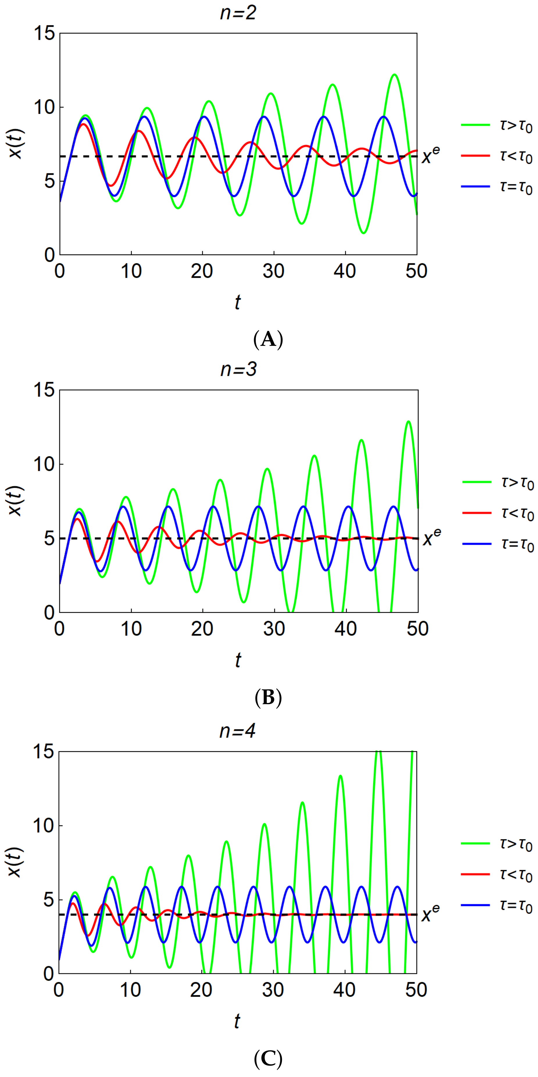
We perform simulations with three different values of $n,n=2,n=3$, and $n=4$. The simulations are done with Mathematica, ver. 12.1. The corresponding critical values of $\tau$ are

$${\tau }_0^{*}\left(2\right)=\frac{2\pi }{3},{\tau }_0^{*}\left(3\right)=\frac{\pi }{2}\mathrm{and}{\tau }_0^{*}\left(4\right)=\frac{2\pi }{5}$$

which imply that the stability region becomes smaller as n increases. This is also clear from the form of ${\tau }_0^{*}\left(n\right)$ in Theorem 1. In each simulation below, we take $\tau ={\tau }_0^{*}\left(n\right)-0.2$ for the red convergent curve and $\tau ={\tau }_0^{*}\left(n\right)+0.1$ for the divergent green curve and assume constant functions for $t\le 0$.

In duopoly, the initial functions are defined as

$${\phi }_1\left(t\right)=x_1^e-3\mathrm{and}{\phi }_2\left(t\right)=x_2^e-2\mathrm{for}t\le 0.$$

In tiropoly and quartopoly, the appropriate functions are similarly defined and the initial values are selected from the neighborhood of the equilibrium point. Although it is clear that the simulation results strongly depend on the model’s specification, we can see the followings from those simulations illustrated in Figure 2A–C:

Figure 2. (A) Oscillatory dynamics in duopoly. (B) Oscillatory dynamics in triopoly. (C) Oscillatory dynamics in quartopoly.

(1)

Theorem 1 is numerically confirmed for $n=2,3,4$; it is seen that the Cournot equilibrium is stable for $\tau <{\tau }_0^{*}\left(n\right),$ loses stability, and bifurcates to a cyclic oscillation for $\tau ={\tau }_0^{*}\left(n\right)$.

(2)

The trajectories are oscillatory because only complex roots can solve the characteristic equations.

(3)

It is further confirmed that the trajectories are oscillatory expanding for $\tau >{\tau }_0^{*}\left(n\right)$ and thus sooner or later become negative, losing economic meaning.

(4)

The time at which the negative production takes place the first time becomes smaller as n increases. Indeed, the green curve first crosses the horizontal axis at $t\simeq 32.012$ in triopoly in Figure 2B and at $t\simeq 25.423$ in quartopoly in Figure 2C. Although it is not illustrated in Figure 2A, the trajectory becomes negative at $t\simeq 59.641$ in duopoly.

Results (3) and (4) are inevitable because the best reply functions are linear and the resultant dynamical system does not have enough nonlinearities to prevent the trajectories from becoming negative. We also have essentially the same results in the case of different delays.

4. Growth Rate Dynamics

In this section, we make one modification to the delay best reply dynamical system, (1), and pursue the possibility of bounded dynamics when the system includes some nonlinearities. In particular, the growth rate adjustment is assumed in which the growth rate of output is controlled by the difference between the optimal output and the actual output,

$$\frac{{\dot{x}}_i\left(t\right)}{x_i\left(t\right)}=k\left[\alpha -x_i(t-{\tau }_1)-\beta \sum _{j\ne i}^n{x}_j(t-{\tau }_2)\right]\mathrm{for}i=1,2,\dots ,n.$$

(11)

System (11) has the same stationary point as system (1). The homogeneous part of its linearized version is

$${\dot{x}}_i\left(t\right)=K\left[-x_i(t-{\tau }_1)-\beta \sum _{j\ne i}^n{x}_j(t-{\tau }_2)\right]\mathrm{for}i=1,2,\dots ,n,$$

(12)

where

$$K=k{x}^e.$$

Comparing (12) with (2) reveals that only the adjustment parameters are different. Thus, the formulas for the critical delays in (4), (5), (7) and (8) obtained in the best reply dynamic system can be applied to the growth rate dynamical system (12) if k is replaced with $K$.

The remaining part of this section is divided into two. The stability switching curves under the growth rate dynamics are constructed and numerical simulations are performed in the first subsection. The stability index is examined to provide theoretical backgrounds with the directions of stability switches for the numerical results in the second part.

4.1. Stability Switching Curves

It is assumed henceforth that K replaces k. Then the pairs of (${\tau }_1^{+}(\omega ,{\ell }_1),{\tau }_2^{-}(\omega ,{\ell }_2)$) and (${\tau }_1^{-}(\omega ,{\ell }_1),{\tau }_2^{+}(\omega ,{\ell }_2)$) in (4) and (5) satisfy the following characteristic equation,

$$\lambda +K{e}^{-\lambda {\tau }_1}-K\beta e^{-\lambda {\tau }_2}=0$$

(13)

where the definitions of ${\theta }_1$ and ${\theta }_2$ should be changed to

$${\theta }_1\left(\omega \right)={cos}^{-1}\left[\frac{4{\omega }^2+3K^2}{8K\omega }\right],$$

(14)

$${\theta }_2\left(\omega \right)={cos}^{-1}\left[\frac{4{\omega }^2-3K^2}{4K\omega }\right]$$

(15)

and the interval $\omega$ is redefined by

$$I=\left[\frac{1}{2}K,\frac{3}{2}K\right].$$

We then have two sets of line segments in the first quadrant of the (${\tau }_1,{\tau }_2$) plane,

$$L_1^{+}({\ell }_1,{\ell }_2)=\left\{\left.({\tau }_1^{+}(\omega ,{\ell }_1),{\tau }_2^{-}(\omega ,{\ell }_2))\right|\omega \in I,({\ell }_1,{\ell }_2)\in \mathit{Z}\right\}$$

(16)

and

$$L_1^{-}({\ell }_1,{\ell }_2)=\left\{\left.({\tau }_1^{-}(\omega ,{\ell }_1),{\tau }_2^{+}(\omega ,{\ell }_2))\right|\omega \in I,({\ell }_1,{\ell }_2)\in \mathit{Z}\right\}$$

(17)

similar to the case of best reply dynamics. Lemma 1 characterizes the relations of the segments $L_1^{+}({\ell }_1,{\ell }_2)$ and $L_1^{-}({\ell }_1,{\ell }_2)$ for the extreme values of $\omega$ in interval I.

Lemma 1.

$L_1^{+}({\ell }_1,{\ell }_2+1)=L_1^{-}({\ell }_1,{\ell }_2)$ holds for the initial point of I, $\omega =K/2,$ and $L_1^{-}({\ell }_1,{\ell }_2)=L_1^{+}({\ell }_1,{\ell }_2)$ holds for the terminal point of I, $\omega =3K/2$.

Proof. 

Substituting $\omega =K/2$ into (14) and (15) gives

$${\theta }_1(K/2)={cos}^{-1}\left(1\right)=0\mathrm{and}{\theta }_2(K/2)={cos}^{-1}(-1)=\pi$$

implying that

$${\tau }_1^{\pm }(K/2,{\ell }_1)=\frac{2}{K}\left(\frac{3}{2}\pi +\left(2{\ell }_1-1\right)\pi \right)$$

and

$${\tau }_2^{+}(K/2,{\ell }_2+1)={\tau }_2^{-}(K/2,{\ell }_2)=\frac{2}{K}\left(\frac{1}{2}\pi +2{\ell }_2\pi \right).$$

Hence $L_1^{+}({\ell }_1,{\ell }_2+1)=L_1^{-}({\ell }_1,{\ell }_2)$ at the initial point of I. In the same way, for $\omega =3K/2,$

$${\theta }_1(3K/2)={cos}^{-1}\left(1\right)=0\mathrm{and}{\theta }_2(3K/2)={cos}^{-1}\left(1\right)=0$$

implying that

$${\tau }_1^{+}(3K/2,{\ell }_1)={\tau }_1^{-}(3K/2,{\ell }_1)=\frac{2}{3K}\left(\frac{3}{2}\pi +\left(2{\ell }_1-1\right)\pi \right)$$

and

$${\tau }_2^{-}(3K/2,{\ell }_2)={\tau }_2^{+}(3K/2,{\ell }_2)=\frac{2}{3K}\left(\frac{1}{2}\pi +\left(2{\ell }_2-1\right)\pi \right).$$

Hence $L_1^{+}({\ell }_1,{\ell }_2)=L_1^{-}({\ell }_1,{\ell }_2)$ at the terminal point of I. This completes the proof. □

Pairs of (${\overline{\tau }}_1^{+}\left(m_1\right),{\overline{\tau }}_2^{-}\left(m_1\right)$) and (${\overline{\tau }}_1^{-}\left(m_2\right),{\overline{\tau }}_2^{+}\left(m_2\right)$) from (7) and (8) satisfy the characteristic equation,

$$\lambda +K{e}^{-\lambda {\tau }_1}+K\beta (n-1)e^{-\lambda {\tau }_2}=0$$

(18)

where the definitions of ${\overline{\theta }}_1$ and ${\overline{\theta }}_2$ should be changed to

$${\overline{\theta }}_1\left(\omega \right)={cos}^{-1}\left[\frac{4{\omega }^2-K^2\left(n-3\right)\left(n+1\right)}{8K\omega }\right]$$

(19)

and

$${\overline{\theta }}_2\left(\omega \right)={cos}^{-1}\left[\frac{4{\omega }^2+K^2\left(n-3\right)\left(n+1\right)}{4K(n-1)\omega }\right]$$

(20)

and the interval for $\omega$ is defined, respectively, by

$$I_2=\left[\frac{1}{2}K,\frac{3}{2}K\right]\mathrm{if}n=2$$

and

$$I_n=\left[\frac{n-3}{2}K,\frac{n+1}{2}K\right]\mathrm{if}n\ge 3.$$

We also have two line segments of (${\tau }_1,{\tau }_2$),

$$L_2^{+}(m_1,m_2)=\left\{\left.({\overline{\tau }}_1^{+}(\omega ,m_1),{\overline{\tau }}_2^{-}(\omega ,m_2))\right|\omega \in I_2\mathrm{or}{I}_n,(m_1,m_2)\in \mathit{Z}\right\}$$

(21)

and

$$L_2^{-}(m_1,m_2)=\left\{\left.({\overline{\tau }}_1^{-}(\omega ,m_1),{\overline{\tau }}_2^{+}(\omega ,m_2))\right|\omega \in I\mathrm{or}{I}_n,(m_1,m_2)\in \mathit{Z}\right\}$$

(22)

similarly to the case of best reply dynamics. Similarly to Lemma 1, we have the followings:

Lemma 2.

In the case of $n=2,L_2^{+}(m_1,m_2+1)=L_2^{-}(m_1,m_2)$ holds for the initial point of $I_2$, $\omega =K/2,$ and $L_2^{-}(m_1,m_2)=L_2^{+}(m_1,m_2)$ holds for the terminal point of $I_2$, $\omega =3K/2$.

Notice that for $n=3,$

$$\underset{\omega \to 0}{lim}{\tau }_1^{\pm }(\omega ,m_1)=\infty \mathrm{and}\underset{\omega \to 0}{lim}{\tau }_2^{\pm }(\omega ,m_2)=\infty .$$

The equality of the segments does not hold at the initial point of $I_3$ but only at the terminal point which can be proved similarly to Lemma 1.

Lemma 3.

In the case of $n=3,L_2^{+}(m_1,m_2)=L_2^{-}(m_1,m_2)$ holds for the terminal point of $I_3$, $\omega =2K.$

If $n\ge 4$, then the following result holds.

Lemma 4.

In the case of $n\ge 4,L_2^{+}(m_1,m_2)=L_2^{-}(m_1+1,m_2)$ holds for the initial point of $I_n$, $\omega =(n-1)K/2$ and $L_2^{+}(m_1,m_2)=L_2^{-}(m_1,m_2)$ holds for the terminal point $\omega =(n+1)K/2$.

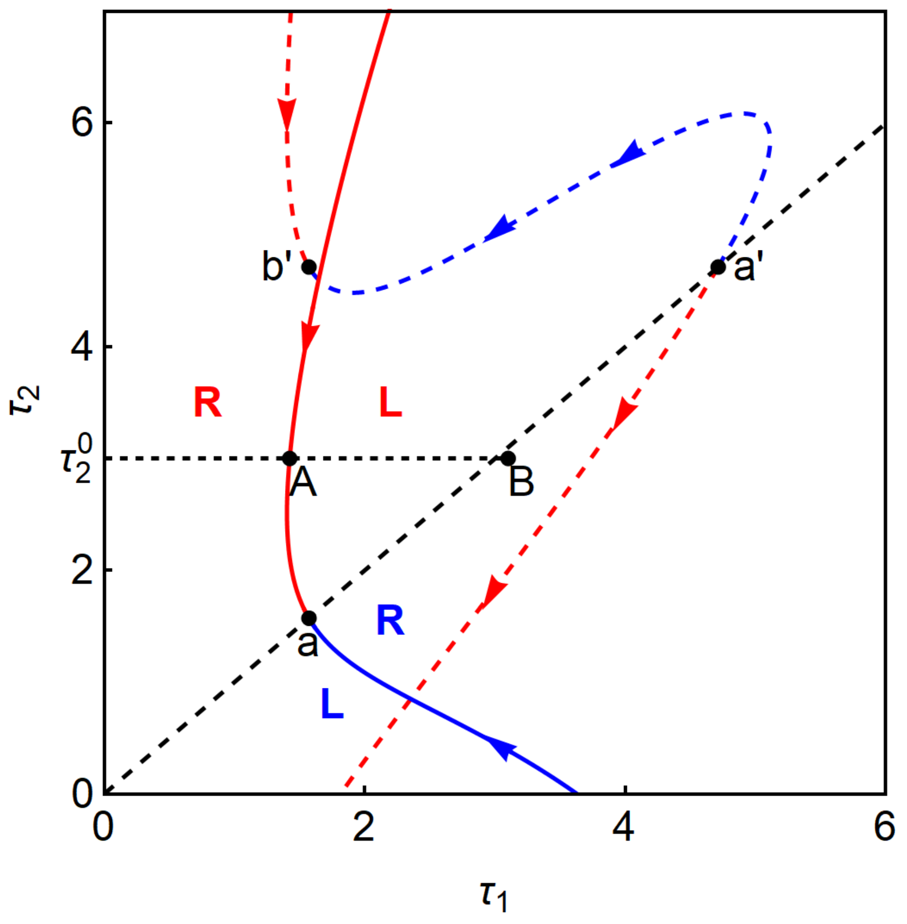
In the following, we will construct stability switching curves. To this end, we specify the parameters’ values as $\alpha =10$ and $k=0.1.$ In Figure 3, the dotted red loci are described by $L_1^{-}({\ell }_1,{\ell }_2)$ with ${\ell }_1=0$ and ${\ell }_2=0,1$ and the dotted blue locus by $L_1^{+}(0,1)$. The black point $a^{\prime }$ is the initial point of $L_1^{+}(0,1)$ and $L_1^{-}(0,0)$ and its coordinates are

$$a^{\prime }=\left(\frac{3}{2}\pi ,\frac{3}{2}\pi \right)$$

at which $L_1^{+}(0,1)=L_1^{-}(0,0)$ holds by Lemma 1. The black point $b^{\prime }$ is the terminal point of $L_1^{+}(0,1)$ and $L_1^{-}(0,1)$ and its coordinates are

$$b^{\prime }=\left(\frac{1}{2}\pi ,\frac{3}{2}\pi \right)$$

at which $L_1^{+}(0,1)=L_1^{-}(0,1)$ holds by Lemma 1. The blue and red solid curves are described by $L_2^{+}(0,0)$ and $L_2^{-}(0,0).$ They are connected at point a,

$$a=\left(\frac{1}{2}\pi ,\frac{1}{2}\pi \right)$$

at which $L_2^{+}(0,0)=L_2^{-}(0,0)$ by Lemma 2.

Figure 3. Stability switching curve (SSC) with $n=2$.

The dotted and solid curves are smoothly connected as is seen in Figure 3. As a result, the (${\tau }_1,{\tau }_2$) region is divided into two subregions by the stability switching curve connecting the left-most parts among the segments of $L_2^{\pm }(0,0),L_1^{\pm }(0,1)$, and $L_1^{-}(0,1).$ As the Cournot equilibrium is stable when there are no delays, it is stable in the region including the origin and left to the connecting curve.

We want to investigate the influence of ${\tau }_1$ and ${\tau }_2.$ Two simulations in the case of $n=2$ are performed with initial functions,

$${\phi }_1\left(t\right)=x_1^e-2\mathrm{and}{\phi }_2\left(t\right)=x_2^e+1\mathrm{for}t\le 0.$$

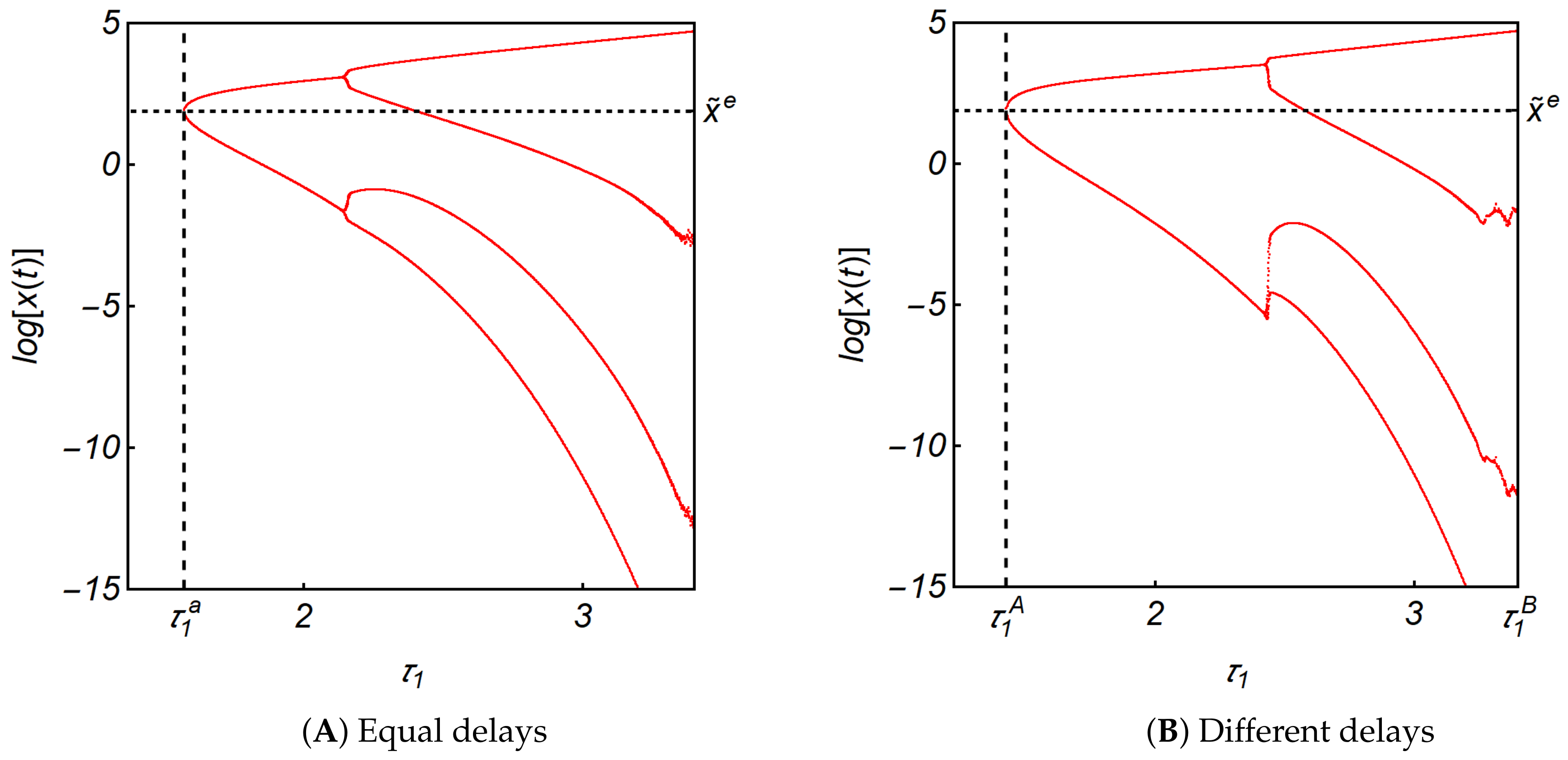
The first simulation result along the diagonal is presented in Figure 4A. The delays increase from ${\tau }_i=0$ to ${\tau }_i=3.4$ with an increment of $0.003$ along the diagonal. The Cournot equilibrium is asymptotically stable for smaller delays and becomes unstable through a Hopf bifurcation at

$${\tau }_i^a={\tau }_0^{*}\left(2\right)=\frac{1}{2}\pi \mathrm{for}i=1,2,$$

producing a limit cycle that further bifurcates to a multi-periodic cycle for larger delays. The second result with the different two delays is given in Figure 4B. The value of ${\tau }_1$ increases from ${\tau }_1={\tau }_1^A\left(\simeq 1.423\right)$ to ${\tau }_1={\tau }_1^B(=3.4)$ along the dotted horizontal line at ${\tau }_2=3$. More precisely, the bifurcation diagrams with two delays are constructed in the following procedure with Mathematica, version 12.1. The value of ${\tau }_2$ is fixed at $3,$ and the value of ${\tau }_1$ is increased from ${\tau }_{min}={\tau }_1^A$ to ${\tau }_{max}={\tau }_1^B$ with an increment $({\tau }_{max}-{\tau }_{min})/1000$. For each value of ${\tau }_1,$ dynamic system (11) runs for $0\le t\le T(=2000),$ and the data for $t\le T-100$ are discarded to get rid of the initial disturbance. The local maxima and minima out of the remaining data are plotted against this ${\tau }_1$ value. Then the value of ${\tau }_1$ is increased and then the same procedure is repeated until ${\tau }_1$ arrives at ${\tau }_{max}.$ The following bifurcation diagrams are obtained in the same way. The resulting bifurcation diagram shows that the dynamic system experience similar dynamics. The stability of the equilibrium point is confirmed for the zero delay and holds for ${\tau }_1<{\tau }_1^A$ and ${\tau }_2=3.$ In both diagrams (and the following diagrams), notation ${\tilde{x}}^e=log\left[x^e\right]$ is used.

Figure 4. Bifurcation diagrams with $n=2$.

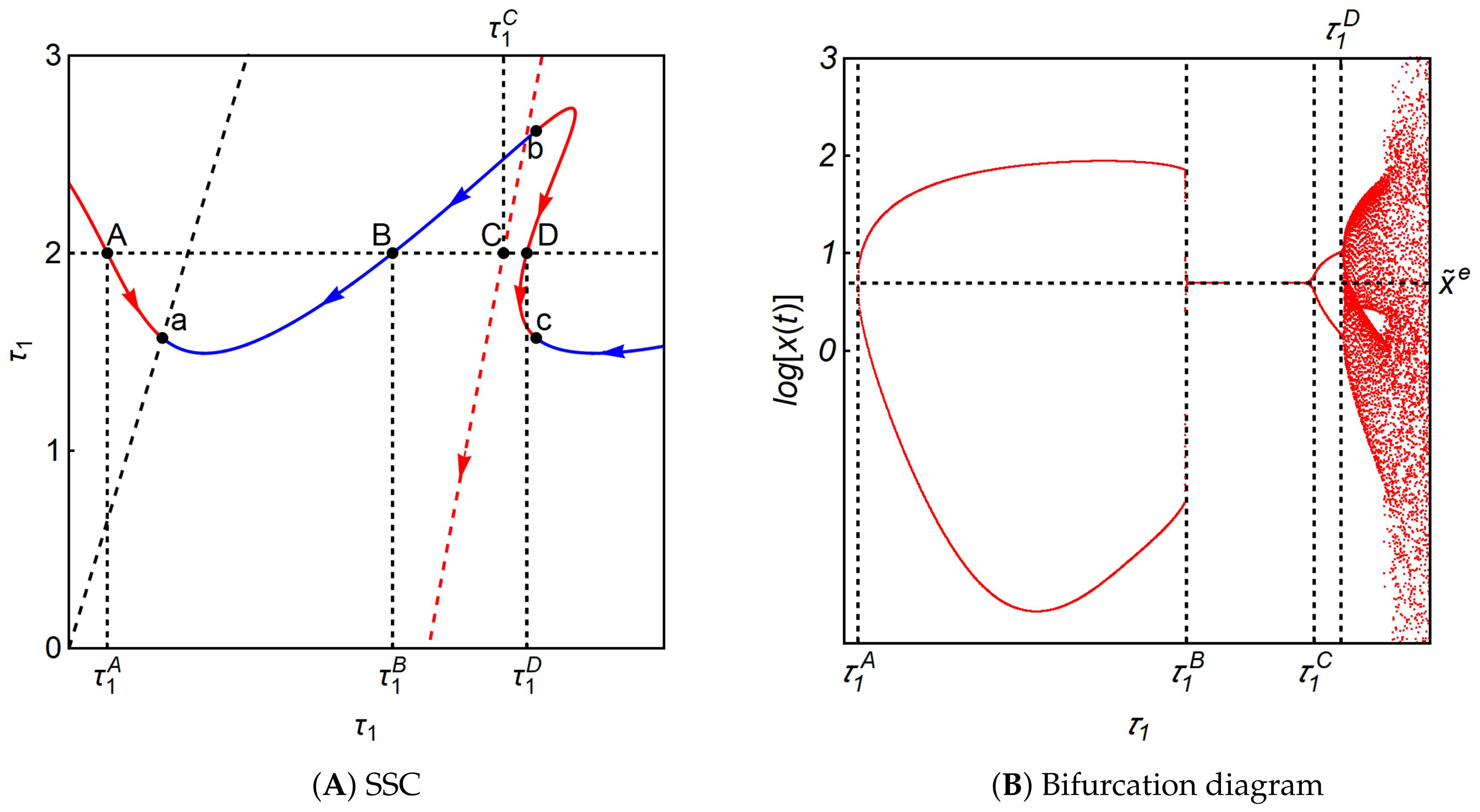
We now increase the number of firms to $3.$Figure 5A shows the stability switching curves. The line segments of $L_2^{+}(0,0)$ (i.e., the solid blue curve) and $L_2^{-}(0,0)$ (i.e., the solid red curve) take the L-shaped profile and rotate counter-clockwise at point a to the extent that the solid red curve is located furthermost to the left. By Lemma 4, both line segments head to point $a,$ the terminal point as $\omega$ increases to $2K.$ We simulate the model (11) along the diagonal (i.e., ${\tau }_1={\tau }_2$) and the dotted horizontal line at ${\tau }_2=3$ (i.e., ${\tau }_1\ne {\tau }_2$) in Figure 5A. As we find qualitatively no big differences between these simulation results as in Figure 4A,B, we depict only the bifurcation diagram with different delays in Figure 5B. It is seen that alá “period-doubling bifurcation” occurs in which the Cournot equilibrium is asymptotically stable for ${\tau }_1<{\tau }_1^A$(≃1.136), loses stability at ${\tau }_1={\tau }_1^A$ and bifurcates to a limit cycle from which new limit cycles emerge having a doubled period of the cycle as ${\tau }_1$ increases from ${\tau }_1^A.$ We also see that further increasing ${\tau }_1$ gives rise to complicated dynamics that suddenly shrinks to a limit cycle with multiple local maxima and minima at some critical point.

Figure 5. Dynamic properties of Equation (11) with $n=3$.

In the case of $n=4$, as is seen in Figure 6A, the solid red and blue segments rotate counter-clockwise further at point a, leading to that the red segment crosses the vertical axis. In Figure 6B, we see that the bifurcation diagram gets more complicated and various dynamics can emerge.

Figure 6. Dynamic properties of Equation (11) with $n=4$.

Lastly, we simulate system (11) with $n=9.$ The shape of the stability switching curve is different from those with smaller n. In Figure 7A, the positive-sloping dotted line is the diagonal, the dotted-red line is $L_2^{-}(0,0)$ as before and the black dots are the starting or ending points of the segments. A remarkable difference is that the solid red-blue segments consist of the wave-shaped curve. Accordingly, the bifurcation diagram is obtained along the horizontal dotted line at ${\tau }_2=2$ and exhibits a different route to chaos. The stability of the Cournot equilibrium is lost at ${\tau }_1={\tau }_1^A$ (≃0.646), regained at ${\tau }_1={\tau }_1^B$ (≃5.441), and then lost again at ${\tau }_1={\tau }_1^C$ (≃7.306). Unstable oscillatory trajectories get complicated for ${\tau }_1>{\tau }_1^D$ (≃7.697). It is known that time delays destabilize dynamic systems. This simulation, however, indicates that time delays can also stabilize the systems.

Figure 7. Dynamic properties of Equation (11) with $n=9$.

Dynamic system (11) examines the birth of complicated dynamics through a period-doubling bifurcation and the occurrence of stability loss and gain. Needless to say, time delays play prominent roles. In addition, taking account of the fact that only the firm’s number is different in those numerical studies, the larger number could influence the system’s dynamics by increasing the degree of interactions among the firms.

4.2. Stability Index

We compute the stability index to provide a theoretical background for finding directions of stability switches. First, we denote the second and third vectors of (3) by $Q_1$ and $Q_2,$

$$Q_1=a_1\left(i\omega \right)e^{-i\omega {\tau }_1}=-i\frac{K}{\omega }\left(cos\omega {\tau }_1-isin\omega {\tau }_1\right)$$

and

$$Q_2=a_2\left(i\omega \right)e^{-i\omega {\tau }_2}=i\frac{K\beta }{\omega }\left(cos\omega {\tau }_2-isin\omega {\tau }_2\right).$$

Having $Q_1$ and $Q_2,$ we further denote the real and imaginary parts by the followings:

$$R_1=\mathrm{Re}{Q}_1=-\frac{K}{\omega }sin\omega {\tau }_1\mathrm{and}{I}_1=\mathrm{Im}{Q}_1=-\frac{K}{\omega }cos\omega {\tau }_1$$

and

$$R_2=\mathrm{Re}{Q}_2=\frac{K\beta }{\omega }sin\omega {\tau }_2\mathrm{and}{I}_2=\mathrm{Im}{Q}_2=\frac{K\beta }{\omega }cos\omega {\tau }_2.$$

Finally, the stability index is defined as follows:

$$\begin{array}{ccc}\hfill S& =& R_2{I}_1-R_1{I}_2\hfill \\ & =& \frac{K^2\beta }{{\omega }^2}\left(sin\omega {\tau }_{1}cos\omega {\tau }_2-cos\omega {\tau }_{1}sin\omega {\tau }_2\right),\hfill \end{array}$$

hence

$$S=\frac{K^2\beta }{{\omega }^2}sin\left[\omega \left({\tau }_1-{\tau }_2\right)\right].$$

(23)

In the same way, we denote the second and third vectors of (6) by ${\overline{Q}}_1$ and ${\overline{Q}}_2,$

$${\overline{Q}}_1=b_1\left(i\omega \right)e^{-i\omega {\tau }_1}=-i\frac{K}{\omega }\left(cos\omega {\tau }_1-isin\omega {\tau }_1\right)$$

and

$${\overline{Q}}_2=b_2\left(i\omega \right)e^{-i\omega {\tau }_2}=-i\frac{K\beta (n-1)}{\omega }\left(cos\omega {\tau }_2-isin\omega {\tau }_2\right).$$

The real and imaginary parts are the followings:

$${\overline{R}}_1=\mathrm{Re}{\overline{Q}}_1=-\frac{K}{\omega }sin\omega {\tau }_1\mathrm{and}{\overline{I}}_1=\mathrm{Im}{\overline{Q}}_1=-\frac{K}{\omega }cos\omega {\tau }_1$$

and

$${\overline{R}}_2=\mathrm{Re}{\overline{Q}}_2=-\frac{K\beta (n-1)}{\omega }sin\omega {\tau }_2\mathrm{and}{\overline{I}}_2=\mathrm{Im}{\overline{Q}}_2=-\frac{K\beta (n-1)}{\omega }cos\omega {\tau }_2,$$

moreover, the stability index is as follows:

$$\begin{array}{ccc}\hfill \overline{S}& =& {\overline{R}}_2{\overline{I}}_1-{\overline{R}}_1{\overline{I}}_2\hfill \\ & =& -\frac{K^2\beta (n-1)}{{\omega }^2}\left(sin\omega {\tau }_{1}cos\omega {\tau }_2-cos\omega {\tau }_{1}sin\omega {\tau }_2\right).\hfill \end{array}$$

Hence

$$\overline{S}=-\frac{K^2\beta (n-1)}{{\omega }^2}sin\left[\omega \left({\tau }_1-{\tau }_2\right)\right].$$

(24)

We call the direction of the curve that corresponds to increasing $\omega$ the positive direction. We also call the region on the left-hand side the region on the left when we head in the positive direction of the curve. Region on the right is defined similarly. Concerning the stability changes, we have the following result from Matsumoto and Szidarovszky (2018) that is based on Gu et al. (2005):

Theorem 2.

Let $\left({\tau }_1,{\tau }_2\right)$ be a point on the stability switching curves, when $i\omega$ is a simple pure complex eigenvalue. Assume we look toward increasing values of ω on the curve, and a point $\left({\tau }_1,{\tau }_2\right)$ moves from the region on the right to the region on the left. A pair of eigenvalues crosses the imaginary axis to the right if $S>0$ or $\overline{S}>0$. If $S<0$ or $\overline{S}<0$, then crossing is in the opposite direction.

The condition of the theorem is satisfied if all $i\omega$ egenvalues are single. It can be proved that the multiple eigenvalues, if any, are isolated from each other, so do the corresponding points on the stability switching curve. Hence at these points, the directions of stability switching are the same as those in the points of their neighborhoods.

We now compute the stability index on the solid red segment of the stability switching curve in Figure 3. The red segment is a locus of the following points,

$$L_2^{-}(0,0)=\left\{\left.\left({\overline{\tau }}_1^{-}(\omega ,0),{\overline{\tau }}_2^{+}(\omega ,0)\right)\right|\omega \in \left[\frac{1}{2}K,\frac{3}{2}K\right]\right\}$$

From (7) and (8), we have

$$\begin{array}{ccc}\hfill \omega \left({\overline{\tau }}_1^{-}(\omega ,0)-{\overline{\tau }}_2^{+}(\omega ,0)\right)& =& \left[\frac{3}{2}\pi -\pi -{\overline{\theta }}_1\left(\omega \right)\right]-\left[\frac{3\pi }{2}-\pi +{\overline{\theta }}_2\left(\omega \right)\right]\hfill \\ & =& -\left[{\overline{\theta }}_1\left(\omega \right)+{\overline{\theta }}_2\left(\omega \right)\right]\hfill \end{array}$$

implying

$$sin\left[\omega \left({\tau }_1-{\tau }_2\right)\right]=-sin\left[{\overline{\theta }}_1\left(\omega \right)+{\overline{\theta }}_2\left(\omega \right)\right]<0$$

when ${\theta }_1+{\theta }_2<\pi$. If ${\theta }_1+{\theta }_2=\pi ,$ then the triangle reduces to a line such that

$$\left|a_1\left(i\omega \right)\right|-\left|a_2\left(i\omega \right)\right|=\pm 1.$$

That is, in Equation (13),

$$\frac{K}{\omega }-\frac{K\beta }{\omega }=\frac{K}{2\omega }=1$$

showing that $\omega =\pi /2$ being the left endpoint of interval I, given for $\omega$, which gives the common starting point of two line segments. In the case of Equation (18),

$$\frac{K}{\omega }-\frac{K\beta (n-1)}{\omega }=\frac{K}{\omega }\left(\frac{3-n}{2}\right).$$

If $n=2,$ this equals $+1$ if $\omega =K/2,$ which is the initial point of I. If $n=3,$ then this expression is always zero, so cannot be $+1$ or $-1$. If $n>3$, then this expression can be only $-1$, when $\omega =K(n-3)/2$, which is the left endpoint of interval $I_n$ which gives again the common starting point of two line segments. In these points, the direction of stability switching is the same as that in the two connecting segments. So in the rest of the discussion, we will assume that ${\theta }_1+{\theta }_2<\pi$. Hence the stability index $\overline{S}$ is positive on the solid red segments of the stability switching curve. In Figure 3, the arrows on the solid red segment indicate the positive direction and the red R and L mean the right and left regions along the red segment. As (${\tau }_1,{\tau }_2$) moves from the R-region to the L-region and $\overline{S}>0$, Theorem 2 implies that a solution pair of (18) crosses the imaginary axis to the right. That is, stability is lost. As seen in Figure 4B, the stability is lost at point A with ${\tau }_1={\tau }_1^A$ when ${\tau }_1$ increases along the horizontal dotted line at ${\tau }_2^0=3.$

Similarly, we can compute the stability index on the solid blue segment,

$$L_2^{+}(0,0)=\left\{\left.\left({\overline{\tau }}_1^{+}(\omega ,0),{\overline{\tau }}_2^{-}(\omega ,0)\right)\right|\omega \in \left[\frac{1}{2}K,\frac{3}{2}K\right]\right\}.$$

From (7) and (8) with K,

$$\begin{array}{ccc}\hfill \omega \left({\overline{\tau }}_1^{+}(\omega ,0)-{\overline{\tau }}_2^{-}(\omega ,0)\right)& =& \left[\frac{3}{2}\pi -\pi +{\overline{\theta }}_1\left(\omega \right)\right]-\left[\frac{3\pi }{2}-\pi -{\overline{\theta }}_2\left(\omega \right)\right]\hfill \\ & =& {\overline{\theta }}_1\left(\omega \right)+{\overline{\theta }}_2\left(\omega \right).\hfill \end{array}$$

Then

$$sin\left[\omega \left({\overline{\tau }}_1^{+}(\omega ,0)-{\overline{\tau }}_2^{-}(\omega ,0)\right)\right]=sin\left[{\overline{\theta }}_1\left(\omega \right)+{\overline{\theta }}_2\left(\omega \right)\right]>0.$$

The stability index $\overline{S}$ is negative,

$$\overline{S}=-\frac{K^2\beta (n-1)}{{\omega }^2}sin\left[{\overline{\theta }}_1\left(\omega \right)+{\overline{\theta }}_2\left(\omega \right)\right]<0.$$

The blue L and R denote the right-region and the left-region with respect to the solid blue segment. Hence the stability is lost when a pair of $({\tau }_1,{\tau }_2)$ crosses the blue segment from the L-region to the R-region.

Consider the stability switching on the dotted red segment located in the upper-left corner of Figure 3. The segment is described by

$$L_1^{-}(0,1)=\left\{\left.\left({\tau }_1^{-}(\omega ,0),{\tau }_2^{+}(\omega ,1)\right)\right|\omega \in \left[\frac{1}{2}K,\frac{3}{2}K\right]\right\}.$$

Then

$$\omega \left({\tau }_1^{-}(\omega ,0)-{\tau }_2^{+}(\omega ,1)\right)=-\pi -\left({\theta }_1\left(\omega \right)+{\theta }_2\left(\omega \right)\right).$$

The stability index is positive

$$S=\frac{K^2\beta }{\omega }sin\left[{\theta }_1\left(\omega \right)+{\theta }_2\left(\omega \right)\right]>0$$

showing that crossing these segments from R to $L,$ stability is lost.

In the lower part of Figure 3, there is a small segment of $L_1^{-}(0,0)$ where

$$L_1^{-}(0,0)=\left\{\left.{\tau }_1^{-}(\omega ,0),{\tau }_2^{+}(\omega ,0)\right|\omega \in \left[\frac{1}{2}K,\frac{3}{2}K\right]\right\},$$

so

$$\begin{array}{ccc}\hfill \omega \left({\tau }_1^{-}(\omega ,0)-{\tau }_2^{+}(\omega ,0)\right)& =& \left[\frac{3}{2}\pi -\pi -{\theta }_1\left(\omega \right)\right]-\left[\frac{1}{2}\pi +\pi -{\theta }_2\left(\omega \right)\right]\hfill \\ & =& \pi -\left[{\theta }_1\left(\omega \right)+{\theta }_2\left(\omega \right)\right].\hfill \end{array}$$

Then

$$sin\left[\omega \left({\tau }_1^{-}(\omega ,0)-{\tau }_2^{+}(\omega ,0)\right)\right]=sin\left[{\overline{\theta }}_1\left(\omega \right)+{\overline{\theta }}_2\left(\omega \right)\right]>0$$

meaning that crossing this segment from the stable region, at least one eigenvalue changes the sign of its real part from negative to positive, implying stability loss.

5. Concluding Remarks

In this paper, n-firm dynamic oligopolies were examined without product differentiation and with linear price and cost functions. Continuous time scales were assumed reconsidering the classical dynamic model of McManus and Quandt (1961) with the best response dynamics. Without delays, the equilibrium is always asymptotically stable without delays regardless of the values of the positive adjustment speeds. We examined how this stability is lost when the firms face implementation and information delays. For the sake of mathematical simplicity, it was assumed that the firms have the same marginal costs and identical delays in both types. If these delays are equal, then a single-delay model is obtained. If the delay is sufficiently small, then the equilibrium is oscillatory stable, at the threshold, the trajectories show cyclic behavior and for larger delays, the cycles become expanding. If the delays are different, then in the resulting two-delay case the stability switching curves were first constructed and then the directions of the stability switches were determined. Growth rate dynamics brought nonlinearities into the model, but their linearized version is identical with best response dynamics, so shows similar local dynamics. Numerical results and simulation studies verify and illustrate the theoretical findings.

This research can be continued in two different ways. One is the consideration of different model modifications such as product differentiation, multi-product models, oligopsonies, labor-managed, and rent seeking oligopolies, including market saturation to mention only a few. The other research direction could be to examine nonlinear models, the local dynamics are similar to that of linear models, however with very different global dynamic behavior.

References

- Cournot, A. Recherches sur les Principes Mathématiques de la Théorie des Richessess; Hachette: Paris, France, 1833. [Google Scholar]
- Theocharis, T.D. On the stability of the Cournot solution on the oligopoly problem. Rev. Econ. Stud. 1960, 27, 133–134. [Google Scholar] [CrossRef]
- McManus, M.; Quandt, R. Comments on the stability of the Cournot oligopoly model. Rev. Econ. Stud. 1961, 28, 136–139. [Google Scholar] [CrossRef]
- Okuguchi, K. Expectations and Stability in Oligopoly Models; Springer: Berlin, Germany, 1976. [Google Scholar]
- Okuguchi, K.; Szidarovszky, F. The Theory of Oligopoly with Multi-Product Firms, 2nd ed.; Springer: Berlin, Germany, 1999. [Google Scholar]
- Ćanovas, J.; Puu, T.; Ruiz, M. The Cournot-Theocharis problem reconsidered. Chaos Solitions Fractals 2008, 37, 1025–1039. [Google Scholar] [CrossRef]
- Hommes, C.; Ochea, M.; Tuinstra, J. Evolutionary competition between adjustment processes in Cournot oligopoly: Instability and complex dynamics. Dyn. Games Appl. 2018, 8, 822–843. [Google Scholar] [CrossRef]
- Lampart, M. Stability of the Cournot equilibrium for a Cournot oligopoly model with n-competitors. Chaos Solitions Fractals 2012, 45, 1081–1085. [Google Scholar] [CrossRef]
- Puu, T. On the stability of Cournot equilibrium when the number of competitors increases. J. Econ. Behav. Organ. 2008, 66, 445–456. [Google Scholar] [CrossRef]
- Puu, T. Rational expectations and the Cournot-Theocharis problem. Discret. Dyn. Nat. Soc. 2006, 2006, 32103. [Google Scholar] [CrossRef]
- Matsumoto, A.; Szidarovszky, F. Theocharis problem reconsidered in differentiated oligopoly. Discret. Dyn. Nat. Soc. 2014, 2014, 630351. [Google Scholar] [CrossRef]
- Bischi, G.-I.; Chiarella, C.; Kopel, M.; Szidarovszky, F. Nonlinear Oligopolies: Stability and Bifurcations; Springer: Berlin, Germany, 2010. [Google Scholar]
- Matsumoto, A.; Szidarovszky, F. Dynamic Oligopolies with Time Delays; Springer Nature: Berlin/Heidelberg, Germany, 2018. [Google Scholar]
- Gu, K.; Nicolescu, S.-I.; Chen, I. On the stability crossing curves for general systems with two delays. J. Math. Appl. 2005, 3311, 231–253. [Google Scholar] [CrossRef]
© 2020 by the authors. Licensee MDPI, Basel, Switzerland. This article is an open access article distributed under the terms and conditions of the Creative Commons Attribution (CC BY) license (http://creativecommons.org/licenses/by/4.0/).