Optimising the Preparedness Capacity of Enterprise Resilience Using Mathematical Programming

Abstract

In today’s volatile business arena, companies need to be resilient to deal with the unexpected. One of the main pillars of enterprise resilience is the capacity to anticipate, prevent and prepare in advance for disruptions. From this perspective, the paper proposes a mixed-integer linear programming (MILP) model for optimising preparedness capacity. Based on the proposed reference framework for enterprise resilience enhancement, the MILP optimises the activation of preventive actions to reduce proneness to disruption. To do so, the objective function minimizes the sum of the annual expected cost of disruptive events after implementing preventive actions and the annual cost of such actions. Moreover, the algorithm includes a constraint capping the investment in preventive actions and an attenuation formula to deal with the joint savings produced by the activation of two or more preventive actions on the same disruptive event. The management and business rationale for proposing the MILP approach is to keep it as simple and comprehensible as possible so that it does not require highly mathematically skilled personnel, thus allowing top managers at enterprises of any size to apply it effortlessly. Finally, a real pilot case study was performed to validate the mathematical formulation.

1. Introduction

The frequency and intensity of disasters continue to increase [1], which is why supply chains and enterprises need to be flexible, agile, robust, organised, prepared and active in order to face any crisis in an efficient way.

Some studies and reports say that many organisations go out of business within two or three years after they experience a major disruption [2]. Therefore, companies in today’s volatile business arena need to be designed to incorporate event readiness, provide an efficient and effective response, and be capable of recovering to their original state or even a better post-disaster state. The capacity to do so has been defined as enterprise resilience when it involves the intra-company level or a single company and supply chain resilience when it affects different entities of the supply chain (inter-company level) [3].

Enterprise resilience is the capacity to avoid, absorb, adapt to and recover from disruptions [4]. Woods [5] defined enterprise resilience as the capacity to anticipate unsafe and unexpected events for organisational survival in the face of threats, including preventing or mitigating failures in the system. Along the same line, Gilly et al. [6] understood enterprise resilience as an active capacity of the company to resist an external event, and a more proactive capacity to anticipate events and thus open new development pathways.

From the previous definitions of enterprise resilience, it is observed that one of the main pillars is the capacity of enterprises to anticipate, prevent and prepare in advance for disruptions. Therefore, enterprises should pay attention to their preparedness capacity to bolster resilience. Firms should implement the necessary actions to improve their preparedness capacity, which in turn will enhance their enterprise resilience capacity. The literature reveals that there are two main types of action to face disruptions, depending on the timeline when they are implemented [7]. Mitigation actions are implemented prior to the occurrence of disruptions and are proactive by nature, and contingency policies are reactive, implemented to recover once a disruption has already occurred. This paper is focused on mitigation policies, as they serve to improve the preparedness perspective of enterprise resilience. More concretely, the mitigation actions considered in this research are focused on preventing disruptions by implementing preventive actions that will try to reduce (i) the probability of occurrence, (ii) the severity of disruptive events or (iii) both.

Coutu [8] stated that enterprise resilience is an organisation’s ability to face reality with staunchness, make meaning of hardship and improvise solutions from thin air. It is broadly recognised that in order to be resilient, organisations need to have a certain degree of ability to improvise in stressful situations. However, it is also true that resilient organisations need to be prepared for the expected, but more importantly for the unexpected. Then, there is a need to develop preparedness actions to guarantee enterprise resilience to face disruptions. The complexity that enterprises deal with daily makes decision-making for enhancing enterprise resilience non-trivial, and it is best facilitated with the aid of mathematical models. For this reason, the main objective of this paper is to propose a mixed-integer linear programming (MILP) model that offers valuable information to support enterprises in their decision-making process related to enhancing the preparedness capacity to be more resilient.

The remainder of this paper is organised as follows. In Section 2, we review relevant literature. Section 3 defines the data modelling approach to characterize the preparedness capacity from the AS IS and TO BE model perspectives. Section 4 develops a MILP model to optimise the activation of a set of preventive actions that enhance the preparedness capacity to reduce enterprises’ proneness to disruptions. In Section 5, a piloting case study is performed at a company in the foam sector. An analysis of the results is performed to provide the enterprise with valuable information to facilitate the decision-making process regarding the progress of its readiness to face disruptions. Finally, Section 6 concludes the paper and defines further research lines.

2. Literature Foundations

Dalziell and McManus [9], Paries [10] and Haimes et al. [11] studied the emergent properties of resilience and considered that it cannot be directly measured as an assessment of the AS IS status. Nevertheless, it is necessary to analyse, in a certain instance, how much an enterprise is prepared to face specific disruptive events. In addition to this, having a great understanding of the AS IS state is as important as improving the current status towards an enhanced preparedness capacity status (TO BE) to deal with an unstable environment.

The literature review offers attempts to assess and enhance the resilience capacity of enterprises and supply chains. However, most of them are conceptual approaches, which are highly valuable contributions for the scientific knowledge theoretical building but are not practically useful for real application. Table 1 offers an overview of these approaches, as proposed by various authors; the review is based on the work performed by [12] and highlights the limitations hindering their practical application.

Table 1. Analysis of approaches related to enterprise resilience enhancement.

	Reference	Approach Orientation	Scope
	Woods et al. [13]	Conceptual Framework	Enterprise
Approach	This approach is based on the principle that in order to achieve resilience, organizations need support for decisions about production/safety trade-offs. Enterprises require mechanisms to analyse when to relax the pressure on throughput and efficiency goals, i.e., making a sacrifice decision; how to help organizations decide when to relax production pressure to reduce vulnerability. To do so, the authors point out the following aspects: (i) Management commitment, (ii) Reporting culture, (iii) Learning culture, (iv) Preparedness/Anticipation, (v) Flexibility and (vi) Opacity (and its corollary, Observability).
Limitation	L1. Conceptual approach, not practically implementable.
	Dalziell et al. [9]	Indicators	Enterprise
Approach	The authors explain that resilience is a function of the vulnerability and adaptive capacity of the company. They use a systematic view of the company and state that one of the key aspects that defined a system is its purpose. Therefore, since a company is a system, the authors directly relate its resilience capacity with the ability to achieve its objectives and purposes. Companies usually map their mission through a series of key performance indicators (KPIs). The ease with which key performance indicators can drift to undesirable levels of instability is a function of the vulnerability of the system. Furthermore, the time it takes for such performance indicators to recover and achieve resilience is a function of the adaptive capacity.
Limitation	L2. Excessive specificity of the approach. The definition of KPIs based on the mission of the company means that each company has different measurable metrics. This characteristic implies that each enterprise deals with the resilience enhancement in a different way.
	McManus et al. [14]	Indicators/Methodology	Enterprise
Approach	This approach considers that the resilience of an organization involves three main axes: (i) situation awareness, (ii) management of the keystone vulnerabilities of an organization and (iii) the adaptive capacity. Based on these three main pillars, the authors develop the model called Relative Overall Resilience, by defining 15 indicators to assess resilience capacity. An extended version of this study may be found in Lee et al. [15].
Limitations	L2. Excessive specificity of the approach. The 15 indicators used to assess enterprise resilience are defined through case studies of organizations. For this reason, the generalizability of the research results is limited to the organizations participating in these case studies. L3. Resilience assessment but not enhancement. This approach offers information about the resilience profile of a company, but it does not offer any additional information regarding how to improve enterprise resilience.
	Falasca et al. [16]	Indicators	Supply chain
Approach	A simulation-based framework that incorporates the following three determinants of resilience: density, complexity, and node criticality into the process of supply chain design. An updated research related to this area was carried out by Kim et al. [17], who propose a set of a metrics for supply network resilience in terms of the total number of node/arc disruptions.
Limitations	L4. Lack of optimisation It does not incorporate cost data into the agents’ decision-making function, thus limiting the possibilities of performing relevant trade-off analyses. The approach tests supply chain responses to different strategies for improving. disaster resilience but it does not look at the determination of an “optimal” strategy under different conditions.
	Stolker et al. [18]	Indicators	Enterprise
Approach	This attempt applies multi-attribute utility theory to measure the management performance of operational resilience in an organization. The approach analyses some elements such as: understanding mission-critical processes, risk management performance, reward system, and cultural aspects.
Limitations	L4. Lack of optimisation.
	Erol et al. [19]	Conceptual Framework	Supply chain
Approach	Conceptual framework focused on extended enterprises and based on the key attributes of enterprise resilience: agility, flexibility, adaptability, interoperability and connectivity. Achieving resilience requires the application of two enablers: (i) the capability of an enterprise to become more connected and responsive to the environment, stakeholders and competitors; and (ii) the alignment of information technology with business goals.
Limitations	L1. Conceptual approach, not practically implementable.
	Barroso et al. [20]	Methodology/Indicators	Supply Chain
Approach	This approach defines a methodology to assess resilience in SCs through value stream mapping to offer a clear view and understanding of supply chain entities’ actual capabilities. Two performance measures are defined for the assessment: supply chain cost and lead time.
Limitations	L2. Excessive specificity of the approach. This study only analyses a very particular case study. L3. Resilience assessment but not enhancement. This research assesses supply chain resilience; however, it does not suggest strategies to improve this capacity.
	Carvalho et al. [21]	Indicators/Methodology	Supply chain
Approach	This research uses a combination of simulation and a case study to design supply chains more resilient to disturbances. In this research, the simulation study is used to evaluate the effects of strategies on the behaviour of some entities of a Portuguese automotive supply chain and to explore if the strategies are effective in overcoming the negative effects of the disturbance: “supply delay”.
Limitation	L2. Excessive specificity of the approach.
	Cabral et al. [22]	Indicators	Enterprise/Supply chain
Approach	This approach proposes an integrated lean, agile, resilient and green analytic network process model to support decision-making in choosing the most appropriate practices and KPIs to be implemented by companies in a supply chain.
Limitation	L2. Excessive specificity of the approach. Limited number of practices and KPIs.
	Soni et al. [23]	Indicators	Supply chain
Approach	This research proposes a model using graph theory which holistically considers all the major enablers of resilience (supply chain agility, collaboration among players, information sharing, sustainability in supply chain, risk and revenue sharing, trust among players, supply chain visibility, creating risk management culture, adaptive capability and supply chain structure) and their interrelationships for analysis using an interpretive structural modeling approach.
Limitation	L3. Resilience assessment but not enhancement. L4. Lack of optimisation The approach quantifies resilience by a single numerical index but it does not offer insights about how to enhance resilience and which are the best strategies to achieve it.
	Munoz et al. [24]	Indicators	Supply chain
Approach	Proposal of a model to assess a set of metrics for operational supply chain resilience in terms of recovery, impact, performance loss, profile length, and weighted-sum.
Limitation	L2. Excessive specificity of the approach. This approach is limited in scope to a serial three-tier supply chain with no backlog.

Apart from the previous attempts, we have only found one contribution that offers a more practical approach, namely the Supply Chain Resilience Assessment and Management (SCRAM^TM) tool defined by [25]. By measuring vulnerability factors such as turbulence, deliberate threats, external pressures, and resource limits, among others, and capability factors such as flexibility, efficiency, visibility, and adaptability, among others, the tool provides an evaluation of the resilience in a supply chain. However, the main limitation is related to its industry-specificity or even firm and product-level particularities, which requires the definition of more specialized metrics. Although these tools shed light on assessing resilience, the resilience subject is under-researched and warrants further study.

Based on the analysis performed in Table 1, some limitations regarding published enterprise and supply chain resilience research have been identified. These main limitations, as well as how the present research will deal with them, are presented in Table 2.

Table 2. Advances beyond the state of the art (SoA).

Limitations	Progress Beyond the SoA
L1. Conceptual approach, not practically implementable.	This research defines a simple but effective MILP that can be applied without difficulty in any enterprise. The mathematical formulation has been proposed from a management and business perspective in order to make it as simple and comprehensible as possible so that it does not require highly mathematically skilled personnel, thus allowing top managers to apply it easily. Moreover, a pilot case study has been performed in a real company to validate the mathematical formulation and to show how the mathematical formulation could be applied.
L2. Excessive specificity of the approach.	The present research is based on Sanchis et al. [12] framework that encompasses 71 disruptive events that enterprises consider as threats to their continuity. Moreover, the current version of the framework also provides a set of 403 preventive actions from among whom to choose the most adequate actions to prepare in advance for disruptive events. The framework has been defined as a living approach. New disruptive events and preventive actions that companies wish to analyse may be included whenever required. Besides, it is important to highlight the generality of the approach taken in this research that allows it to be applied to any type of company, of any size and sector. Finally, the mathematical formulation offers a generic and easy-to-use mechanism to guarantee that it can be applied effortlessly.
L3. Resilience assessment but not enhancement.	Most of the studies found in the literature review are mainly focused on measuring how resilient organisations are, but they do not offer guidelines and/or recommendations on how to enhance the resilience capacity. The present research optimises the activation of a set of preventive actions that enhance the preparedness capacity to reduce enterprises’ proneness to disruptions and offers valuable information to support enterprises in their decision-making process aimed at becoming more resilient.
L4. Lack of optimisation

From a mathematical viewpoint, there are also very few approaches related to (i) enterprise resilience enhancement and (ii) the improvement of its constituent capacities: preparedness, adaptive and recovery. Manopiniwes and Irohara [26] developed a stochastic linear mixed-integer programming model for integrated decisions in the preparedness and response stages of pre- and post-disaster operations, taking into account three key areas of emergency logistics: facility and stock prepositioning, evacuation planning and relief vehicle planning. Sanchis and Poler developed a quantitative approach to enhance enterprise resilience by selecting optimal preventive actions using dynamic programming [27].

The use of sourcing strategies to achieve supply chain resilience under disruptions based on the definition of a scenario-based mathematical model including disruption risks and operational risks was developed in [28]. Other studies, such as [29], propose an optimisation model, and its solution determines the rerouting strategy for product flow through the supply chain under disruptions.

Other efforts have been made towards the development of fuzzy mathematical models, such as that defined in [30] for assessment of organisational resilience potential in small to medium-sized enterprises (SMEs) of the process industry. Other studies use fuzzy Delphi techniques such as [2], which defined an integrated Delphi–fuzzy logic framework for measuring SC resilience, and [31] which applied fuzzy Delphi mechanisms and a fuzzy best–worst method to identify and prioritize the relevant disaster resilience indicators for SMEs. A fuzzy linear programming enterprise input–output model was developed in [32] to determine optimal adjustments in production levels of multi-product systems when a crisis is induced by a loss of resource inputs. Another work related to resilience and mathematical modelling is that developed in [33] with the definition of a fuzzy multicriteria decision-making approach (using a fuzzy analytic hierarchical process and the fuzzy Technique for Order Preference by Similarity to Ideal Solution) to evaluate and rank organisational resilience factors with respect to user preference orders.

Tukamuhabwa et al. [34] stated that only limited research has been conducted on choosing and implementing an appropriate set of strategies to improve the capacity of resilience. Moreover, research in enterprise and supply chain resilience covers only specific contexts, such as disaster relief (e.g., [1]) and particular areas such sourcing, routing or production (e.g., [28,29,32], respectively). Based on this, and to the best of our knowledge, there have been only a very few studies addressing the optimisation of the resilient capacity of organisations to face disruptions, and those that are found are specifically focused on specific contexts and particular crises. Shirali et al. [35] also stated that sophisticated safety management systems have contributed to decreasing the number of usual accidents, but these classical approaches may not have been sufficient to prevent the occurrence of extraordinary incidents such as the COVID-19 pandemic that we are currently experiencing. There is no clear answer as to how to overcome such high-impact but low-probability events. However, it seems that some companies cope far better than others when they are resilient [36]. Consequently, there is a need for new approaches to enhance the resilience capacity.

For all these aspects, this paper proposes a mathematical formulation to optimise the implementation of actions that enhance the preparedness capacity to be more resilient. This research is based on the enterprise resilience conceptual reference framework defined by Sanchis et al. [12], shown in Figure 1. The framework is composed of three main sections:

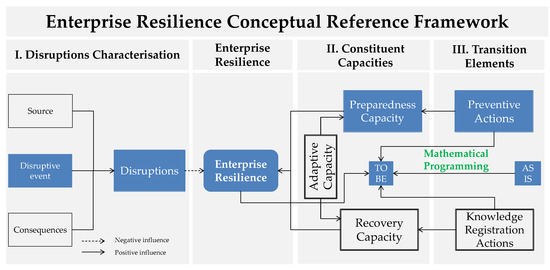
Figure 1. Enterprise resilience conceptual reference framework (based on [12]).

• Disruption characterisation
  This section, based on the categorisation framework of disruption defined in [37], is in turn composed of the following:
  • Source, divided into (i) the level at which the disruptive event originated and (ii) the origin and suborigin of the disruptive event. More information can be found in [38].
  • Disruptive event per se, considered as a situation that causes a disturbance to a company’s daily operations. The framework contains 71 of the most common disruptive events suffered by companies.
  • Consequences, which are a set of related effects that a specific disruptive event occurrence may cause.
• Constituent capacity
  In order to deal with the negative effects of disruptions, companies should be as resilient as possible. To accomplish this, the framework is focused on three main capacities of enterprise resilience:
  • Preparedness: the readiness capacity to face disruptions, assessing whether companies have the knowledge, means and resources to be able to anticipate different disruptions [39].
  • Adaptivity: defined as the degree to which the system can modify its circumstances and move towards a condition of stability [40]. Sandanam et al. [41] defined it as the capacity to respond to challenges through learning, managing risk and impacts, developing knowledge, and devising novel solutions. The dynamic nature of adaptive capacity allows companies to be prepared in advance and recover after having been impacted by a disruptive event. Following [42], the dynamism of adaptive capacity is the reason why it is considered in the framework as an intrinsic characteristic of the capacities of preparedness and recovery and not a constituent capacity, per se, of enterprise resilience.
  • Recovery: the ability to respond to and bounce back from a disruptive situation, which is key to bolstering enterprise resilience.
• Transition elements
  In order to enhance preparedness and recovery capacities, companies need to take different actions. In the first case, the framework proposes preventive actions as proactive mechanisms to face inevitable disruptive events. In the second case, the framework points to knowledge management to guarantee that the necessary knowledge is available to be reused when necessary and facilitate the recovery process.
  • Preventive actions are policies and/or actions that are carried out in an attempt to reduce the probability of the occurrence or severity of a disruptive event or both [20]. They are proactive by nature. In case of inevitable disruptive events, effort should be focused on mitigating the negative consequences.
  • Regarding knowledge registration actions, Dalziell et al. [9] explained that one of the ways in which a system can recover from adverse situations is to apply available responses to deal with disruptive events. To do so, profound knowledge of the available responses to disruptive events that have already occurred is required in order to reuse the knowledge generated in past recovery actions.

In summary, when a disruptive event occurs, a company is pushed from a state of relative equilibrium to another state characterised by instability. The ease with which the enterprise is moved to this new unstable state is a measure of its vulnerability [9], understood as a lack of preparedness capacity to deal with disruptive events, while the ease with which the enterprise responds is a measure of its recovery capacity. In both cases, companies will be more prepared and will recover more efficiently if they adapt more easily to changes. In order to enhance the preparedness and recovery capacities of enterprise resilience, the framework defines as proactive mechanisms the preventive actions to anticipate and be prepared for disruptive events and the knowledge registration actions to ensure that knowledge is available when required for reactive purposes. As mentioned above, this paper is only focused on mitigation policies, as they are the ones that will serve to improve the preparedness perspective of enterprise resilience. Figure 1 shows all the elements of the enterprise resilience conceptual reference framework; only the ones in blue, related to preparedness capacity, are analysed in this study through mathematical programming.

3. Data Modelling Approach

This section defines the data modelling approach to characterize preparedness capacity from the AS IS and TO BE model perspectives. Figure 2 shows a summary of the data-modelling approach, which consists of three main sections: (i) data definition, (ii) nomenclature definition and (iii) transformation of the data into the nomenclature used for application in the mathematical formulation through data processing.

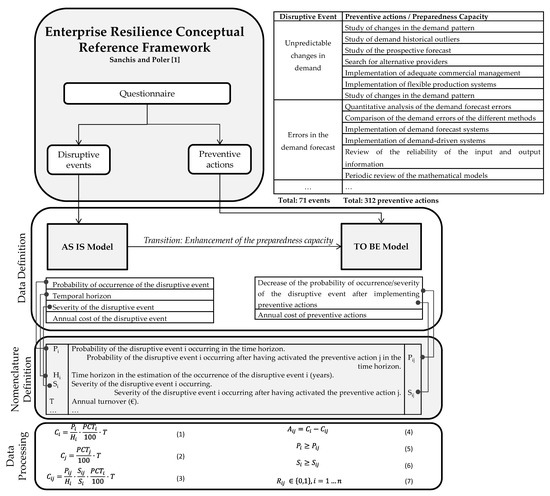
Figure 2. Data-modelling approach.

3.1. Data Definition

The necessary data to quantify the current preparedness capacity status (AS IS) and related to the future ideal situation (TO BE) were gathered through a questionnaire. The study of Munoz and Dunbar [24] utilised disruptions as experimental inputs for their simulation model. Our research also identifies disruptions as the main element to analyse the preparedness capacity of enterprise resilience. A framework for data collection was designed and a questionnaire was developed to facilitate the process of data capture. The current version of the questionnaire contains 71 disruptive events to be analysed.

Tukamuhabwa et al. [34] identified a wide range of strategies for improving resilience, focusing on increasing flexibility, creating redundancy, forming collaborative supply chain relationships and improving supply chain agility. However, such a proposal does not offer concrete actions to be implemented to improve the capacity of resilience. To overcome this, and based on the conceptual framework developed in [12], the present research offers, by defining specific preventive actions per disruptive event, a set of concrete actions to be activated in order to enhance the pre-disruption capacity of enterprise resilience. Tarafdar and Qrunfleh [43] theoretically explained and empirically demonstrated how information systems’ capability for agility also contributes to effecting a positive relationship between agile supply chain strategy and supply chain performance. For this reason, many of the preventive actions defined are related to information systems to build resilient companies. Currently, the framework for data collection offers 403 preventive actions.

The disruptive events included in the framework were identified and selected based on an exhaustive literature review, in which the most worrisome disruptive events were identified. Two types of bibliographical source were used in this identification. Firstly, the scientific literature was reviewed. However, studies focused on identifying the most common risks are scarce [4,20,44,45,46,47,48]. For this reason, alternative information sources were used. This second type of information was obtained from reports published by well-known consulting firms that issue risk-ranking studies annually [49,50,51,52,53,54,55,56,57].

The definitions of the preventive actions were based on two approaches: (i) the conceptual approach, in which for each disruptive event, the most appropriate preventive actions were identified based on the literature review, and (ii) a Delphi study, in which a panel of experts collaborated to assess the set of preventive actions defined in the previous phase. Besides the assessment, the experts also proposed more preventive actions based on their experience and background. This iterative process was repeated in two consecutive rounds until the results obtained were the same and the assessment was finished.

3.1.1. Definition of Input Data Required to Analyse the AS IS State

The necessary input data were divided into two main streams, one related to the AS IS situation and one that covers the TO BE situation. Table 3 offers an overview of the required information of the current status in order to analyse preparedness capacity.

Table 3. Input data required to analyse current (AS IS model) preparedness capacity.

AS IS Situation	Description
Probability of occurrence of disruptive event	The likelihood that a disruptive event will occur. Enterprises have to estimate the probability of occurrence according to a 5-level Likert scale (very high (VH), high (H), medium (M), low (L), and very low (VL)). Based on studies performed by Lichtenstein and Newman [58], Moore [59], Boehm [60], Hamm [61], Conrow [62] and Hillson [63], whose main aim was to determine the numerical values for each scale range, the present research uses values proposed in [63]: VH, 80.1%; H, 64.5%; M, 43.3%; L, 18%; and VL, 8.1%.
Temporal horizon	The time horizon, defined as a future point in time when the occurrence of disruptive events will be evaluated. In this research, three temporal horizons are considered: long-term (more than 10 years), medium-term (between 5 and 10 years, average 5 years) and short-term (next year). Quantification of the time horizon is used to differentiate between more and less habitual disruptive events at the same probability level.
Severity of disruptive event	The most likely consequences of a potential disruptive event. In other words, the harshness assigned to the consequences if a specific disruptive event materializes. Severity is assessed through a 5-level Likert scale in the same way as probability of occurrence. In light of this, the numerical values of severity levels are based on previous works developed by Fine [64], Dickson [65], Romero et al. [66] and Smith [67]. In this research, the values for severity are the averages defined by Patterson and Neailey [68]: VH, 95.5%; H, 70.5%; M, 35.5%; L, 13.0%; and VL, 2.5%.
Annual cost of disruptive event	The monetary amount that it would cost if a specific disruptive event materialised. If the company is working at a normal level of operation and a disruptive event occurs, this cost is the amount of money that the company will have to invest to return from the unstable state to the normal state of operation. Users of the questionnaire provide this piece of information as a percentage of annual turnover.

3.1.2. Definition of Input Data Required to Analyse TO BE Situation

Once the current preparedness capacity has been characterised and it is shown how vulnerable an enterprise is, a roadmap should be defined. This roadmap will include a set of optimal preventive actions to be implemented to achieve the ideal future situation in relation to the ability to be prepared in advance to face disruptive events.

The necessary input data to characterise the TO BE situation and define the roadmap are shown in Table 4.

Table 4. Input data required to analyse future (TO BE model) preparedness capacity.

TO BE Situation	Description
Decreased probability of occurrence/severity of disruptive event	The main goal of implementing preventive actions is to diminish the probability of occurrence and/or the severity of disruptive events. Therefore, it is necessary to estimate the new range to which the probability and severity are reduced in order to quantify the improvement after such actions.
Annual cost of preventive actions	The annual cost of implementing/activating a specific preventive action. The following assumptions are considered with regard to preventive actions: The cost of preventive actions will always be lower than the cost of disruptive events. Otherwise, companies would never implement them, since it would be more profitable to let disruptive events happen. Preventive measures will always reduce the probability of occurrence and/or severity of disruption. Otherwise, it would not be necessary to invest in them; it would be better to wait for the impact and then apply recovery policies. The cost of a specific preventive action is estimated annually. For example, implementing information backups need an initial investment of €10,000. The enterprise estimates that yearly maintenance will cost €1000 and this backup system will be used for 5 years, so the annual cost of the preventive action will be €3000. For other preventive actions that must be implemented repeatedly every year, estimating the annual cost is much easier. The data are provided as a percentage of the company’s annual turnover.

3.2. Nomenclature Definitions

Table 5 shows the nomenclature used to define the MILP model.

Table 5. Nomenclature of mixed-integer linear programming (MILP) model.

Indices
i	Disruptive events that may potentially occur
j	Preventive actions for enhancing preparedness capacity to face disruptive events
Parameters
Pi	Probability of disruptive event i occurring in the time horizon
Pij	Probability of disruptive event i occurring after implementing preventive action j in the time horizon
Hi	Time horizon for estimating the occurrence of disruptive event i (years)
Si	Severity of disruptive event i
Sij	Severity of disruptive event i after implementing preventive action j
T	Annual turnover (€)
PCTi	Cost of disruptive event i as % of annual turnover if it occurs
PCTj	Cost of preventive action j as % of annual turnover
Rij	Binary parameter that relates disruptive event i and preventive action j
Ci	Expected annual cost of disruptive event i (€)
Cj	Annual cost of preventive action j (€)
Cij	Expected annual cost of disruptive event i after implementing preventive action j (€)
Aij	Annual savings by implementing preventive action j for disruptive event i (€)
Decision variables
Ej	Binary variable indicating whether preventive action j is activated or not (1 if activated, 0 if not)
CDi	Expected annual cost of disruptive event i after implementing one or several preventive actions j (€)
Ai	Annual savings by activating one or several preventive actions for disruptive event i (€).

3.3. Data Processing

The questionnaire allows users to provide information for only those disruptive events they wish to analyse, which allows enterprises to solely focus on the main worrisome disruptive events. However, as mentioned above, the data provided through the questionnaire by end users need to be processed in order to be used as input data for MILP. Taking into account that companies provide cost information through the questionnaire as a percentage of annual turnover, the expected annual cost of disruptive event i is calculated by (1):

$$C_i=\frac{P_i}{H_i}·\frac{PC{T}_i}{100}·T.$$

(1)

In the same way, the annual cost of preventive action j is calculated as indicated in (2):

$$C_j=\frac{PC{T}_j}{100}·T.$$

(2)

The expected annual cost of disruptive event i after implementing preventive action j is shown in (3):

$$C_{ij}=\frac{P_{ij}}{H_i}·\frac{S_{ij}}{S_i}·\frac{PC{T}_i}{100}·T.$$

(3)

Therefore, if the company implements preventive actions that enhance its preparedness capacity, the cost of the disruptive event is estimated to be lower, which will result in savings according to (4):

$$A_{ij}=C_i-C_{ij}.$$

(4)

It is assumed that the probability of occurrence of a disruptive event is equal to or higher than the probability of occurrence of the same event after a preventive action is implemented. In light of this, the same applies to severity, as shown in (5) and (6):

$$P_i\ge P_{ij},$$

(5)

$$S_i\ge S_{ij}.$$

(6)

In addition, R_ij is a binary parameter that indicates the relationship between disruptive event i and preventive actions j. If the value of R_ij is 1, preventive action j has a relationship with disruptive event i, reducing its probability of occurrence and/or severity. If the value of R_ij is 0, it means that preventive action j has no influence on disruptive event i, as indicated in (7):

$$R_{ij} \in \left\{0,1\right\}, i=1\dots n.$$

(7)

4. Mixed-Integer Linear Programming Model

This section formulates the mathematical programming by defining the MILP model following the nomenclature described in Section 3.2.

The objective function of Model (8) is to minimize the expected annual cost of disruptive events after implementing preventive actions, and the annual cost of preventive actions to be implemented is calculated as:

$$Minimize z= {\displaystyle \sum }_{i=1}^{n}C{D}_i+{\displaystyle \sum }_{j=1}^m{C}_j·E_j$$

(8)

Subject to the following:

Constraint (9) ensures that the total cost of preventive actions to be implemented is less than the monetary resources the company is willing to invest to enhance its preparedness capacity, that is, investment in enterprise resilience:

$${\displaystyle \sum }_{j=1}^m{C}_j·E_{j }\le I.$$

(9)

Constraint (10) calculates the expected annual cost of disruptive event i after implementing preventive actions as the difference between the expected annual cost and the annual savings that the disruptive event would generate after one or several preventive actions are activated. This value cannot be less than zero.

$$C{D}_i\ge C_i- A_i 1\le i\le n$$

(10)

Constraint (11), involving a formula that calculates a measured quantity, indicates the total savings the company would experience in the disruptive event analysed after implementing the preventive actions by E_j = 1.

$$A_i={\displaystyle \sum }_{j=1}^m{A}_{ij}·R_{ij}·E_j, 1\le i\le n$$

(11)

However, there is an aspect to be considered when a combination of preventive actions that affect the same disruptive event is activated. In this case, improvements in terms of savings are not necessarily the sum of savings provided by all activated preventive actions. This can be illustrated with examples related to the analysis of combined drug effects [69]. The study of dose-effect relationships when multiple drugs are used [70] presents the same casuistry as the analysis of the saving-effect relationship when multiple preventive actions are activated. Following this research stream, we found that Belen’kii et al. [71] defined the antagonistic drug concept (or depotentiation, negative interaction, negative synergy, etc.) as the joint effect of two or more drugs in such a way that the combined effect is less than the sum of the effects produced by each agent separately [72,73]. Based on this pattern, and as suggested in [27], the antagonism related to preparedness capacity is considered as joint savings produced by the activation of two or more preventive actions in such a way that the combined savings is less than the sum of the savings produced by each preventive action separately.

One potential solution to overcome the antagonism effect is to ask enterprises through the questionnaire about the savings generated by different combinations of preventive actions. However, based on their experience, enterprises reported that this solution was not practicable because the estimation process is complex and time-consuming. For this reason, an attenuation formula of savings after activating two or more preventive actions for the same disruptive event was defined. The attenuation formula is based on research by Sanchis and Poler [27] and is expressed in (12):

$${\mu }_i=\alpha ·\frac{\beta }{k_i}$$

(12)

where α is a parameter between 0 and 1; β is a parameter between 0 and k_i; and $k_i$ is the number of preventative actions activated for the same disruptive event i. The values of α and β will depend on the degree to which the end user wishes to attenuate the savings when more than one preventive action is activated.

When the MILP model is computed and the optimal solution is obtained, if two or more preventive actions are activated for the same disruptive event, the attenuation formula is applied, and the model is recalculated successively until there is no further attenuation. The attenuation algorithm iteratively applies MILP to calculate the optimal set of preventive actions j (optimal set of E_j values) based on the previous A_ij values. If MILP results in changes to E_j, savings A_ij for each disruptive event i is then attenuated by factor μ_i, which corresponds to the updated E_j value (bar the largest Aij for each event i). MILP is recalculated with the updated A_ij values until two equal consecutive solutions are obtained. To validate the MILP model with an exploratory approach, a case study of a company is presented in Section 5.

5. Application to a Foam Company

This application involves an international company that designs, engineers, and provides advanced foam solutions for a wide range of technical applications from insoles for footwear to soundproofing solutions for the building industry. The company operates across Europe, North America and Asia and its headquarters are located in eastern Spain.

5.1. Input Data

The company participating in this case study was interested in analysing four types of disruptive events, those related to supply (S), environment (ET), finances (F) and legislation (L), with a total of 21 disruptive events studied. Moreover, the company chose 83 preventive actions as mitigation actions to improve its preparedness capacity. A summary of the disruptive events related to supply aspects and the preventive actions to be activated is shown in Table 6 [74]. In this case, the enterprise wanted to analyse 7 events and selected 28 preventive actions to prepare in advance to face such events.

Table 6. Summary of disruptive events related to supply aspects and preventive actions (based on [74]).

#D	Disruptive Event	#A	Preventive Actions
S1	Poor quality of raw materials or components supplied	S1.1	Search for alternative raw materials or components
		S1.2	Search for alternative suppliers
		S1.3	Certify (audit) supplier quality
		S1.4	Implement quality systems agreed with suppliers
		S1.5	Conduct pre-production inspection
		S1.6	Maintain safety stock
S2	Limiting changes in capacity of suppliers	S2.1	Search for alternative suppliers
		S2.2	Define long-term contractual agreements with suppliers
		S2.3	Implement continuous monitoring systems of suppliers/materials
		S2.4	Adopt backward vertical integration
S3	Geographic dispersion of suppliers (time difference, language, proximity)	S3.1	Search for alternative suppliers
		S3.2	Promote closer relationships
		S3.3	Implement real-time communication systems
S4	Delay in supply of raw materials or components	S4.1	Implement penalties for delays
		S4.2	Search for alternative suppliers
		S4.3	Encourage collaborative work with suppliers and joint problem-solving to establish realistic replenishment systems
		S4.4	Maintain safety stock
S5	Shortage of raw materials	S5.1	Search for alternative raw materials or components
		S5.2	Define new compositions of products
		S5.3	Define complementary products that do not require scarce raw materials and replace current products
		S5.4	Implement reverse logistics and recycling systems
S6	Price fluctuations of materials supplied	S6.1	Analyse seasonality and trends (supply-demand balance) of raw material prices
		S6.2	Search for alternative raw materials or components
		S6.3	Search for alternative suppliers
		S6.4	Closely monitor commodity markets; make strategic purchases
S7	Withdrawal of key supplier	S7.1	Increase the supply base
		S7.2	Partner with suppliers (temporary union of companies)
		S7.3	Use vertical backward integration of all or part of the supply function

In the case of environmental and context-related events, the enterprise was also willing to analyse 7 events, for a total of 27 proposed preventive actions, as shown in Table 7.

Table 7. Summary of disruptive events related to environmental and context-related aspects and preventive actions.

#D	Disruptive Event	#A	Preventive Actions
ET1	Fire	ET1.1	Train personnel on security measures for fire protection
		ET1.2	Ensure constant revision and maintenance of fire hoses
		ET1.3	Maintain insurance contracts that include anti-fire clauses
		ET1.4	Implement anti-fire measures
		ET1.5	Conduct periodic fire drills
ET2	Increase of competitors	ET2.1	Conduct periodic analysis of the competition
		ET2.2	Use benchmarking
		ET2.3	Define differentiation strategies from competitors
ET3	Entry of new competitors in emerging countries	ET3.1	Analyse potential patents and intellectual property rights to protect products/processes of focal firm
		ET3.2	Define policies that foster creation of high reputation and brand loyalty of focal firm
		ET3.3	Define product differentiation policies
ET4	Facilities are exposed to severe natural disasters	ET4.1	Define business continuity plans
		ET4.2	Define emergency evacuation protocols
		ET4.3	Train personnel in security measures for protection
		ET4.4	Conduct periodic drills
		ET4.5	Simulate disaster scenarios and establish specific measures based on simulation results
ET5	Geopolitical instability in countries where enterprise has facilities	ET5.1	Define a structured, analytical and comparative approach to potential political changes and government policies around the world
		ET5.2	Define and analyse indicators related to degree of uncertainty in strategic countries that could lead to adverse changes in operations of focal firm
		ET5.3	Conduct strategic planning regarding locations of new facilities of focal firm considering the situation of governments in such countries
		ET5.4	Simulate geopolitical scenarios and establish specific measures based on simulation results
ET6	Industrial espionage	ET6.1	Define policies to periodically change passwords and protocols that allow access to different levels of information
		ET6.2	Define employment contracts with formal descriptions of activities that can be considered as espionage (or may favour it due to the absence of due diligence) and specify consequences for workers
		ET6.3	Have specific and constantly updated protection programs (anti-spyware, antivirus, firewall)
ET7	Sabotage, theft, vandalism, kidnapping and extortion	ET7.1	Develop educational programme for physical protection of facilities
		ET7.2	Control and register dissatisfied employees or those who often have a negative attitude against regulations established by focal firm
		ET7.3	Establish policies to promote satisfaction of personnel of focal firm
		ET7.4	Establish efficient system of identifying, registering and controlling persons, packages and vehicles

With regard to financial issues, the enterprise selected 4 disruptive events as the most worrisome, with 14 preventive actions (Table 8).

Table 8. Summary of disruptive events related to financial aspects and preventive actions.

#D	Disruptive Event	#A	Preventive Actions
F1	Restricted access to credit	F1.1	Create a reserve fund and define policies that maintain a percentage of monetary reserve
		F1.2	Study the viability of turning to supply chain financing instruments
		F1.3	Study and analyse policies supported by public institutions to fund companies (e.g., Official Credit Institute and Enisa in Spain)
		F1.4	Request credit through reciprocal guarantee companies that act as guarantors of financing, assuming credit risks
F2	Changes in interest rates	F2.1	Negotiate with banks on variable interest rate
		F2.2	Study the advisability of investing in products with a fixed interest rate
		F2.3	Study the advisability of investing in or asking for funding to foreign entities or currency (e.g., swiss franc - CHF)
F3	Changes in currency exchange rates	F3.1	Define a standard conversion method to the reference currency when registering accounting information
		F3.2	Define hedging strategies to neutralize or reduce the risk of exposure to fluctuations in exchange rates
		F3.3	Sign contracts for future commercial transactions at an exchange rate agreed upon in the present
F4	Cash problems	F4.1	Search for a sponsor
		F4.2	Create reserve fund and define policies that maintain a percentage of monetary reserve
		F4.3	Study the viability of turning to supply chain financing instruments
		F4.4	Provide inventory liquidation with discount

The last group of disruptive events that the enterprise wanted to analyse is related to legislation issues, with 3 events and 14 preventive actions, as shown in Table 9.

Table 9. Summary of disruptive events related to environmental and context-related aspects and preventive actions.

#D	Disruptive Event	#A	Preventive Actions
L1	New and more restrictive legislation of imports/exports	L1.1	Design and develop flexible, fast and easily reconfigurable processes
		L1.2	Design and develop easily adaptable products that meet the most stringent requirements of new regulations (weight, composition, presentation, identification, labelling)
		L1.3	Participate in lobbying activities exerting pressure to influence decisions about legislation
		L1.4	Monitor import and export trade regimes constantly
		L1.5	Monitor countries under embargo constantly and study alternatives for such countries
L2	Changes in legislation involving changes in company processes	L2.1	Train employees in legal issues
		L2.2	Define and implement publicity activities among customers about potential changes in the focal company’s processes from a positive approach; e.g., more environmentally friendly
		L2.3	Design and develop flexible, fast and easily reconfigurable processes
		L2.4	Implement continuous monitoring systems to control new or existing regulations/laws that could affect company’s processes
		L2.6	Participate in lobbying activities exerting pressure to influence decisions about legislation
L3	Changes in legislation involving changes in our products	L3.1	Train employees in legal issues
		L3.2	Define and implement publicity activities among customers about potential changes in focal company’s products from a positive viewpoint; e.g., higher security
		L3.3	Design and develop easily adaptable products that meet the most stringent requirements of new regulations (weight, composition, presentation, identification, labelling)
		L3.4	Implement continuous monitoring systems to control new or existing regulations/laws that could potentially affect company’s products

In Table 6, three preventive actions apply to different disruptive events, e.g., the preventive action “Search for alternative raw materials or components” (S1.1, S5.1 and S6.2) applies to three different events. The same occurs with preventive actions shown in Table 10.

Table 10. Preventive actions that apply to multiple disruptive events.

D	A	Preventive Action
S1, S5, S6	S1.1, S5.1, S6.2	Search for alternative raw materials or components
S1, S2, S3, S4, S6	S1.2, S2.1, S3.1, S4.2, S6.3	Search for alternative suppliers
S1, S4	S1.6, S4.4	Maintain safety stock
ET1, ET4	ET1.5, ET4.4	Conduct periodic drills
F1, F4	F1.1, F4.2	Create a reserve fund and define policies that maintain a percentage of monetary reserve
	F1.2, F4.3	Study the viability of turning to supply chain financing instruments
L1, L2	L1.1, L2.3	Design and develop flexible, fast and easily reconfigurable processes
	L1.3, L2.6	Participate in lobbying activities exerting pressure to influence decisions about legislation
L1, L3	L1.2, L3.3	Design and develop easily adaptable products that meet the most stringent requirements of new regulations (weight, composition, presentation, identification, labelling)
L2, L3	L2.1, L3.1	Train employees in legal issues
	L2.2., L3.2	Define and implement publicity activities among customers about potential changes in focal company’s processes/products from a positive approach

The C_j of such preventive actions is the same, as they are equal. For this reason, if in the optimal solution one of these preventive actions is activated, the MILP only records C_j once, but the profits of activation, in terms of savings, are applied to all disruptive events to which it is related. From 83 preventive actions selected by the company, only 68 are unique actions.

The data related to the response of the company to the questionnaire is available in Appendix A (Table A1).

In order to compute the company’s responses, the data was processed according to the data of Table 3 and Table 4:

• Temporal horizon: short (S): 1 year; medium (M): 5 years; long (L): 10 years
• Probability: very low (VL): 8.1%; low (L): 18%; medium (M): 43.3%; high (H): 64.5%; very high (VH): 80.1% [63]
• Severity: very low (VL): 2.5%; low (L): 13%; medium (M): 35.5%; high (H): 70.5%; very high (VH): 95.5% [68]

Moreover, if two or more preventive actions are activated for the same disruptive event and attenuation of savings has to be applied, the company defined α as 0.3 and β as 1. It is worth mentioning that the lower α is, the greater the attenuation, and the lower β is, the less the attenuation.

5.2. Implementation and Resolution

The proposed model was developed using Julia for Mathematical Optimisation (JuMP), an algebraic modelling language embedded in Julia, a high-level, high-performance, open-source multi-platform programming language for technical computing. It is dynamically typed, provides multiple dispatch, and is designed for parallelism and distributed computation. It matches the performance of languages such as C and FORTRAN without the hassle of low-level code [75]. In order to select this language, different algebraic modelling languages were analysed, including A Mathematical Programming Language (AMPL), General Algebraic Modeling System (GAMS), Linear, Interactive, and Discrete Optimizer (LINGO) and Mathematical Programming Language (MPL), among others.

JuMP was finally selected, as it is an open-source modelling language that allows users to express a wide range of optimisation problems (linear, mixed-integer, quadratic, conic-quadratic, semidefinite and nonlinear) in a high-level algebraic syntax [76]. Moreover, JuMP takes advantage of advanced features of Julia programming such as user-friendliness, speed, solver independence, access to advanced algorithmic techniques and ease of embedding [75].

The resolution was carried out with Computational Infrastructure for Operations Research (COIN-OR) branch and cut (Cbc) [77], an open-source optimisation solver of mixed-integer programming, programmed in C++.

Finally, it is worth mentioning that the input data and model solution values were processed with MariaDB. The experiment was run on a thin client server with an Intel^® Xeon^® CPU ES-2620 O @2.00 GHz 2.00 GHz processor and 2.00 GB of RAM. The solving time was less than one minute.

5.3. Evaluation of Results

Based on the values of C_i, disruptive events related to environmental aspects such as accidents and manmade circumstances, among others, are the most critical as they represent more than 77% of the expected annual cost of all disruptive events analysed, followed by supply (more than 9%), financial (more than 7%) and legislative events.

Moreover, it is important to highlight that four disruptive events (ET4, ET5, ET1 and ET3) represent 70% of the total expected annual cost of all disruptive events, which means that preventive measures should be addressed to prepare the company to face such events, as long as such actions are optimal (in monetary terms) to improve the current preparedness capacity. To do so, the company participating in this validation is willing to invest €15,000 annually to enhance its preparedness capacity. Through computation of MILP, in 16 of 21 analysed disruptive events, preventive actions are activated. In addition, in five of the events (S1, S6, ET1, ET5 and ET6), more than one preventive action is activated, and for this reason the attenuation formula is applied in order to attenuate the savings of the joint activation of two preventive actions. In this case, MILP is iterated until two consecutive solutions are equal. In this case, and as shown in Table 11, five iterations are needed. Detailed results are available in Appendix A (Table A2).

Table 11. Input data and results of analysis of preparedness capacity of enterprise resilience (costs are in €).

							Iteration 1		Iteration 2		Iteration 3		Iteration 4		Iteration 5
#	#D	$\frac{\mathit{P}\mathit{C}{\mathit{T}}_{\mathit{i}}}{100}·\mathit{T}$	Ci	#	#A	Cj	Ej	CDi	Ej	CDi	Ej	CDi	Ej	CDi	Ej	CDi
1	S1	30.000	19.350	1	S1.1	950	1	0	1	2767	1	2767	1	2767	1	2767
				2	S1.2	900	1		1		1		1		1
				3	S1.3	1500
				4	S1.4	3000
				5	S1.5	550
				6	S1.6	8000
2	S2	7.500	1.350	2	S2.1	900	1	997	1	997	1	997	1	997	1	997
				7	S2.2	500
				8	S2.3	1000
				9	S2.4	7250
3	S3	15.000	2.700	2	S3.1	900	1	452	1	452	1	452	1	452	1	452
				10	S3.2	800
				11	S3.3	1500
4	S4	35.000	6.300	2	S4.2	900	1	3172	1	3172	1	3172	1	3172	1	3172
				6	S4.4	8000
				12	S4.1	1500
				13	S4.3	2500
5	S5	50.000	21.650	1	S5.1	950	1	6644	1	6644	1	6644	1	6644	1	6644
				14	S5.2	6000
				15	S5.3	6800
				16	S5.4	5000
6	S6	10.000	866	1	S6.2	950	1	0	1	278	1	278	1	278	1	278
				2	S6.3	900	1		1		1		1		1
				17	S6.1	500
				18	S6.4	1500
7	S7	8.000	1.032	19	S7.1	900		1032		1032		1032		1032		1032
				20	S7.2	3000
				21	S7.3	7250
8	ET1	400.000	72.000	22	ET1.1	2000	1	5070	1	23,918	1	23,918	1	23,918	1	23,918
				23	ET1.2	4000
				24	ET1.3	20,000
				25	ET1.4	8000
				26	ET1.5	1500	1
9	ET2	15.000	1.935	27	ET2.1	550		1935		1935		1935		1935		1935
				28	ET2.2	400
				29	ET2.3	1500
10	ET3	50.000	40.050	30	ET3.1	8000		12,367		20,167		20,167		20,167		20,167
				31	ET3.2	1.500	1		1		1		1		1
				32	ET3.3	750	1
11	ET4	400.000	173.200	26	ET4.4	1500		1228		0		0		0		3860
				33	ET4.1	1500							1		1
				34	ET4.2	1200					1
				35	ET4.3	800	1		1						1
				36	ET4.5	1250			1		1		1		1
12	ET5	250.000	108.250	37	ET5.1	2000	1	768		768		54,509		54,509		54,509
				38	ET5.2	2000			1
				39	ET5.3	15,000
				40	ET5.4	1250	1		1		1		1		1
13	ET6	75.000	32.475	41	ET6.1	1500		13,500	1	0	1	3229	1	6075	1	3229
				42	ET6.2	350	1		1		1				1
				43	ET6.3	2000
14	ET7	35.000	3.031	44	ET7.1	500		3031		3031		3031		3031		3031
				45	ET7.2	1000
				46	ET7.3	2500
				47	ET7.4	12,000
15	F1	10.000	6.450	48	F1.1	2500		2362		6450		2362		6450		2362
				49	F1.2	800	1				1				1
				50	F1.3	800
				51	F1.4	1500
16	F2	15.000	12.015	52	F2.1	1500		12,015		12,015		12,015		12,015		12,015
				53	F2.2	3000
				54	F2.3	2700
17	F3	8.000	5.160	55	F3.1	550		5160		5160		5160		5160		5160
				56	F3.2	2000
				57	F3.3	1000
18	F4	25.000	16.125	48	F4.2	2500		151		5451		4656		5451		4656
				49	F4.3	800	1				1				1
				58	F4.1	1000	1		1		1		1		1
				59	F4.4	2500
19	L1	15.000	9.675	60	L1.1	8000		1784		1784		1784		1784		1784
				61	L1.2	5000
				62	L1.3	2500
				63	L1.4	1000
				64	L1.5	550	1		1		1		1		1
20	L2	20.000	12.900	60	L2.3	8000		6496		6496		92		92		6496
				62	L2.6	2500
				65	L2.1	600	1		1		1		1		1
				66	L2.2.	2000							1		1
				67	L2.4	1000					1
21	L3	18.000	11.610	61	L3.3	5000		5846		5846		5846		0		5846
				65	L3.1	600	1		1		1		1		1
				66	L3.2	2000							1		1
				68	L3.4	1000
Total CDi								84,010		108,363		154,045		155,928		164,309
Total Cj								14,950		14,900		14,850		15,000		14,950
Total z								98,960		123,263		168,895		170,928		179,259

Table 11 also shows, for each disruptive event and iteration, which preventive actions are activated (E_j = 1) to enhance the preparedness capacity. The CD_i column represents the expected annual cost of disruptive events after activating optimal preventive actions. In the first iteration, disruptive events related to supply and context or the environment are those in which more preventive actions are activated. For disruptive events related to financial aspects, only F1 and F4 benefit from the activation of preventive actions. With regard to legislation aspects, in the three analysed events, preventive actions are applied. After the attenuation of savings when more than one preventive action was activated for the same disruptive event, the CD_i column of iteration 5 shows the final optimal results. Figure 3 shows these results as the decreased C_i percentage after activating the optimal set of preventive actions.

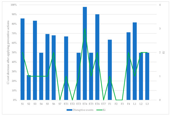
Figure 3. C_i cost decrease after activating k_i preventive actions.

In the case that no preventive actions are activated (e.g., S7, ET2, ET7, F2 and F4), the percentage is null as CD_i = C_ij. The maximum K_i is related to disruptive event ET4. In this case three preventive actions are activated. In disruptive events S1, S6, ET6, F4, L2 and L3, the optimal solution activates two actions and in S2–S5, ET1, F1 and L1, only one action. The attenuation of savings caused by several preventive actions acting on the same disruptive event reduces their attractiveness; in subsequent iterations they may be replaced by other actions that might act on different events. Therefore, the effect of attenuation is diversification in preventive actions activated, thus mitigating a larger share of disruptive events. Figure 4 shows the AS IS and TO BE model in terms of expected annual cost of disruptive events before (AS IS) and after (TO BE) activating one or several preventive actions. The TO BE model has a smaller area than the AS IS model, which means that the decrease in expected annual cost is worth considering. The smaller the area of the TO BE model, the more prepared the company will be to face unforeseen situations related to supply, environmental, financial and legislative issues. Based on Figure 4, the costliest disruptive events are those related to environmental aspects. However, these are also the events for which the annual savings by implementing preventive actions is the highest of the four types. In this case, annual savings account for almost 75% of expected annual cost, followed by supply events, with an annual savings of 71%. The annual savings for legislation aspects is 58%, and events related to financial aspects have less savings: the preventive actions reduce the expected annual cost by only 39% because there are two events (F2 and F3) with no actions.

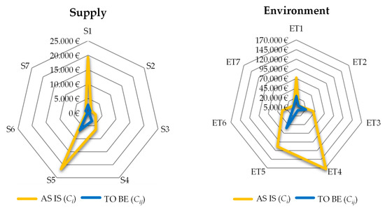
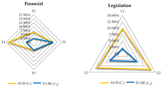
Figure 4. AS IS and TO BE models in terms of in terms of expected annual cost (€) for supply (S), environment (ET), financials (F) and legislation (L) aspects.

All in all, Figure 5 shows the results in an aggregated way. The expected annual cost of the TO BE model is reduced by 70%, without considering the cost of implementing the optimal set of preventive actions, and by 67% considering such cost. In light of this, it is important to highlight that the investment to activate the preventive actions of the optimal solution (C_j) represents only 4% of the reduction in expected annual cost (CD_i – C_ij), demonstrating that a small investment is required to substantially improve the preparedness capacity.

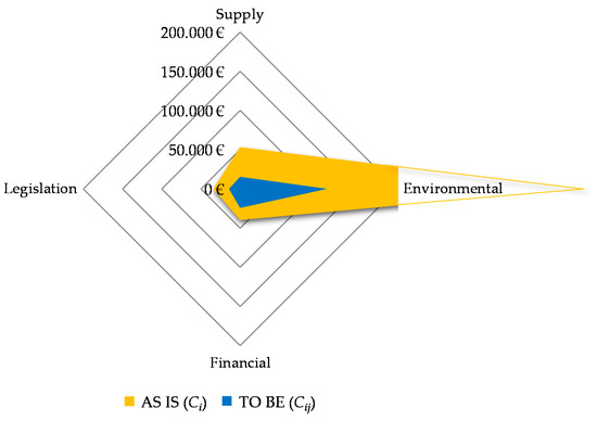
Figure 5. AS IS and TO BE models in terms of in terms of expected annual cost (€).

Finally, we would like to mention, just out of curiosity, that while performing this study (September 2019), the region where the company is located suffered a cold drop (gota fría in Spanish). This is an archaic meteorological term used popularly in Spain which has commonly come to refer to any high-impact rainfall event occurring in the autumn along the country’s Mediterranean coast [78]. This is related to disruptive event ET4. If the company had implemented preventive actions in advance, the effects of the cold drop would have been less, since it would have been more prepared. More information about strategies for improving flood resilience can be found in [79].

6. Conclusions and Further Research

Based on the conceptual reference framework for enhancing enterprise resilience developed in [12], this paper gathered data from a real company, through an online questionnaire, about which disruptive events kept them up at night and which preventive actions they thought were suitable for implementation to enhance their preparedness capacity. In light of this, the company provided specific data related to the AS IS model, that is, their current situation and at what level they would like to be prepared (TO BE model). All of this information was processed to apply the defined MILP model.

The MILP model minimises the expected annual cost of disruptive events after implementing a set of preventive actions and the annual cost of actions to be implemented. Moreover, it considers that enterprises have limited resources to implement such actions. At this point, it is also important to highlight the ease with which mathematical programming provides the optimal solution with a very modest effort.

The results of the application to the real enterprise show that the reduction in expected annual cost is substantial with an investment that, according to the company, does not represent a great effort. Therefore, and based on the results, it seems that the improvement in resilience capacity by enhancing the preparedness capacity is considerable.

Without practical and easy-to-use mechanisms for enhancing the preparedness capacity of enterprise resilience, enterprises will remain reluctant to invest in potentially resilience-enhancing actions and will thus remain vulnerable to disruptions. For this reason, the mathematical approach defined is not very difficult and does not require highly mathematically skilled personnel. The ease of the proposed MILP allows managers to apply it effortlessly. One of the challenges when defining the MILP was to try to define it as simply as possible, in order to facilitate its adoption not only in large companies, but also small and medium-sized enterprises (SMEs) with limited resources. In this way, SMEs could make decisions based on the results of this model to improve their preparedness capacity in advance to face adverse situations. For example, after the hard months following the first coronavirus outbreak, many companies began to take decisions and actions to be prepared for the possibility of a new outbreak. The comprehensibility of the mathematical formulation proposed in this research could be of utmost utility for enterprises of any size to identify the optimal preparatory actions in anticipation of a second COVID-19 outbreak.

From a scientific point of view, this study gives a reason to define a simple but effective approach, allowing top managers to decide which preventive actions are the optimal ones to implement in order to face up to unexpected disruptive events and to improve the proactive perspective of enterprise resilience capacity. The findings of this research suggest that with a small investment in enterprise resilience, it is possible to considerably enhance the preparedness capacity. This shows that preventive actions can be very efficient (cost-savings ratio), thus validating the appropriateness of the actions defined in the framework developed by [12]. According to the case study results, the cost of implementing the preventive actions contemplated in the MILP solution only represents, in this case, 4% of the reduction in the annual expected cost of disruptions, and the enhancement in the preparedness capacity is around 67%. These enticing results might encourage top managers to use this contribution.

Further research will focus on undertaking a sensitivity analysis considering the effect on the outcome of varying the input data. This might help guide managers in prioritizing mitigation strategies that are more economically attractive.

Moreover, the current mathematical formulation offers highly relevant information about the optimal preventive actions to implement in order to improve preparedness capacity. However, it does not provide information about the optimal sequence of implementation. Further research will be focused on working in optimisation and prioritisation of implementation, considering the enterprise’s resource availability over time.

Another research line will be aimed at optimising the preparedness capacity at the inter-company level, that is, involving the whole supply chain. In this case, the focus of optimisation will evolve from an intra-company to an inter-company perspective, taking into account (i) the specific singularities and difficulties of the inter-company level, and (ii) the relationships among various preventive actions to be implemented by different entities of the supply chain. Moreover, it is planned to study how activating preventive actions by a particular entity of the supply chain influences, in a positive or negative way, other entities of the supply network.

References

- Day, J.M. Fostering emergent resilience: The complex adaptive supply network of disaster relief. Int. J. Prod. Res. 2014, 52, 1970–1988. [Google Scholar] [CrossRef]
- Kumar, S.; Anbanandam, R. An integrated Delphi—Fuzzy logic approach for measuring supply chain resilience: An illustrative case from manufacturing industry. Meas. Bus. Excell. 2019, 23, 350–375. [Google Scholar] [CrossRef]
- Ponomarov, S.Y.; Holcomb, M.C. Understanding the concept of supply chain resilience. Int. J. Logist. Manag. 2009, 20, 124–143. [Google Scholar] [CrossRef]
- Madni, A.M.; Jackson, S. Towards a Conceptual Framework for Resilience Engineering. IEEE Syst. J. 2009, 3, 181–191. [Google Scholar] [CrossRef]
- Woods, D.D. Essential Characteristics of Resilience. In Resilience Engineering: Concepts and Precepts; Hollnagel, E., Woods, D.D., Leveson, N., Eds.; Ashgate: Hampshire, UK, 2006; pp. 21–34. [Google Scholar]
- Gilly, J.; Kechidi, M.; Talbot, D. Resilience of organisations and territories: The role of pivot firms. Eur. Manag. J. 2014, 32, 596–602. [Google Scholar] [CrossRef]
- Tomlin, B. On the value of mitigation and contingency strategies for managing supply chain disruption risks. Manag. Sci. 2006, 52, 639–657. [Google Scholar] [CrossRef]
- Coutu, D.L. How Resilience works. Harv. Bus. Rev. 2002, 80, 46–56. [Google Scholar]
- Dalziell, E.; Mcmanus, S.T. Resilience, Vulnerability, and Adaptive Capacity: Implications for System Performance. Int. Forum Eng. Decis. Mak. 2004, 17. [Google Scholar]
- Paries, J. Complexity, Emergence, Resilience. In Resilience Engineering: Concepts and Precepts; Hollnagel, E., Woods, D.D., Leveson, N., Eds.; Ashgate Press: Hampshire, UK, 2006; pp. 43–53. [Google Scholar]
- Haimes, Y.Y.; Crowther, K.; Horowitz, B.M. Preparedness: Balancing Protection with Resilience in Emergent Systems. Syst. Eng. 2008, 11, 287–308. [Google Scholar] [CrossRef]
- Sanchis, R.; Canetta, L.; Poler, R. A Conceptual Reference Framework for Enterprise Resilience Enhancement. Sustainability 2020, 4, 1464. [Google Scholar] [CrossRef]
- Woods, D.; Wreathall, J. Managing Risk Proactively: The Emergence of Resilience Engineering; Ohio University: Columbus, OH, USA, 2003. [Google Scholar]
- Mcmanus, S.; Seville, E.; Brunsdon, D.; Vargo, J. Resilience management: A framework for assessing and improving the resilience of organizations. Resilient. Organ. Res. Rep. 2007, 1, 79. [Google Scholar]
- Lee, V.; Vargo, J.; Seville, E. Developing a tool to measure and compare organizations’ resilience. Nat. Hazards Rev. 2013, 14, 29–41. [Google Scholar] [CrossRef]
- Falasca, M.; Zobel, C.W.; Cook, D. A Decision support framework to assess supply chain resilience. In Proceedings of the 5th International ISCRAM Conference, Washington, DC, USA, 4–7 May 2008; pp. 596–605. [Google Scholar]
- Kim, Y.; Chen, Y.S.; Linderman, K. Supply network disruption and resilience: A network structural perspective. J. Oper. Manag. 2015, 33, 43–59. [Google Scholar] [CrossRef]
- Stolker, R.; Karydas, D.; Rouvroye, J. A comprehensive approach to assess operational resilience. In Proceedings of the Third Resilience Engineering Symposium 2008, Antibes-Juan-les-Pins, France, 28–30 October 2008; pp. 247–253. [Google Scholar]
- Erol, O.; Sauser, B.J.; Mansouri, M. A framework for investigation into extended enterprise resilience. Enterp. Inf. Syst. 2010, 4, 111–136. [Google Scholar] [CrossRef]
- Barroso, A.; Machado, V.H.C. Supply Chain Resilience Using the Mapping Approach. Supply Chain Manag. 2011, 161–184. [Google Scholar]
- Carvalho, H.; Barroso, A.P.; Machado, V.H.; Azevedo, S.; Cruz-Machado, V. Supply chain redesign for resilience using simulation. Comput. Ind. Eng. 2012, 62, 329–341. [Google Scholar] [CrossRef]
- Cabral, I.; Grilo, A.; Cruz-Machado, V. A decision-making model for lean, agile, resilient and green supply chain management. Int. J. Prod. Res. 2012, 50, 4830–4845. [Google Scholar] [CrossRef]
- Soni, U.; Jain, V.; Kumar, S. Measuring supply chain resilience using a deterministic modeling approach. Comput. Ind. Eng. 2014, 74, 11–25. [Google Scholar] [CrossRef]
- Munoz, A.; Dunbar, M. On the quantification of operational supply chain resilience. Int. J. Prod. Res. 2015, 53, 6736–6751. [Google Scholar] [CrossRef]
- Pettit, T.J.; Croxton, K.L.; Fiksel, J. Ensuring supply chain resilience: Development and implementation of an assessment tool. J. Bus. Logist. 2013, 34, 46–76. [Google Scholar] [CrossRef]
- Manopiniwes, W.; Irohara, T. Stochastic optimisation model for integrated decisions on relief supply chains: Preparedness for disaster response. Int. J. Prod. Res. 2017, 55, 979–996. [Google Scholar] [CrossRef]
- Sanchis, R.; Poler, R. Enterprise Resilience Assessment-A Quantitative Approach. Sustainability 2019, 11, 4327. [Google Scholar] [CrossRef]
- Namdar, J.; Li, X.; Sawhney, R.; Pradhan, N. Supply chain resilience for single and multiple sourcing in the presence of disruption risks. Int. J. Prod. Res. 2018, 56, 2339–2360. [Google Scholar] [CrossRef]
- Wang, X.; Herty, M.; Zhao, L. Contingent rerouting for enhancing supply chain resilience from supplier behavior perspective. Int. Trans. Oper. Res. 2016, 23, 775–796. [Google Scholar] [CrossRef]
- Aleksić, A.; Stefanović, M.; Arsovski, S.; Tadić, D. An assessment of organizational resilience potential in SMEs of the process industry, a fuzzy approach. J. Loss Prev. Process Ind. 2013, 26, 1238–1245. [Google Scholar] [CrossRef]
- Fatrias, D.; Hendrawan, D.; Fithri, P.; Rusman, M. An Application of Combined Fuzzy MCDM Techniques in Structuring Disaster Resilience Indicators for Small and Medium Enterprises: A Case Study. In Proceedings of the 2019 IEEE 6th International Conference on Industrial Engineering and Applications, Tokyo, Japan, 12–15 April 2019; pp. 639–643. [Google Scholar]
- Tan, R.; Aviso, K.; Cayamanda, C.; Chiu, A. A fuzzy linear programming enterprise input–output model for optimal crisis operations in industrial complexes. Int. J. Prod. Econ. 2016, 181, 410–418. [Google Scholar] [CrossRef]
- Tadić, D.; Aleksić, A.; Stefanović, M.; Arsovski, S. Evaluation and ranking of organizational resilience factors by using a two-step fuzzy AHP and fuzzy TOPSIS. Math. Probl. Eng. 2014, 2014. [Google Scholar] [CrossRef]
- Tukamuhabwa, B.R.; Stevenson, J.; Busby, J.; Zorzini, M. Supply chain resilience: Definition, review and theoretical foundations for further study. Int. J. Prod. Res. 2015, 53, 5592–5623. [Google Scholar] [CrossRef]
- Shirali, G.A.; Shekari, M.; Angali, K.A. Quantitative assessment of resilience safety culture using principal components analysis and numerical taxonomy: A case study in a petrochemical plant. J. Loss Prev. Process Ind. 2016, 43, 277–284. [Google Scholar] [CrossRef]
- Tang, C.S. Perspectives in Supply Chain Risk Management. Int. J. Prod. Econ. 2006, 103, 451–488. [Google Scholar] [CrossRef]
- Sanchis, R.; Poler, R. Enterprise resilience assessment: A categorisation framework of disruptions. Dir. Organ. 2014, 54, 45–53. [Google Scholar]
- Sanchis, R.; Poler, R. Origins of Disruptions Sources Framework to Support the Enterprise Resilience Analysis. IFAC-PapersOnLine 2019, 52, 2062–2067. [Google Scholar] [CrossRef]
- Sanchis, R.; Poler, R. Definition of a framework to support strategic decisions to improve Enterprise Resilience. IFAC Proc. Vol. (IFAC-PapersOnline) 2013, 46, 700–705. [Google Scholar] [CrossRef]
- Luers, A.L.; Lobell, D.B.; Sklar, L.S.; Addams, C.L.; Matson, A. A method for quantifying vulnerability, applied to the agricultural system of the Yaqui Valley, Mexico. Glob. Environ. Chang. 2003, 13, 255–267. [Google Scholar] [CrossRef]
- Sandanam, A.; Diedrich, A.; Gurney, G.G.; Richardson, T.D. Perceptions of cyclone preparedness: Assessing the role of individual adaptive capacity and social capital in the Wet Tropics, Australia. Sustainability 2018, 10, 1165. [Google Scholar] [CrossRef]
- Christopher, M. Managing risk in the supply chain. Supply Chain Pract. 2005, 7, 4. [Google Scholar]
- Tarafdar, M.; Qrunfleh, S. Agile supply chain strategy and supply chain performance: Complementary roles of supply chain practices and information systems capability for agility. Int. J. Prod. Res. 2017, 55, 925–938. [Google Scholar] [CrossRef]
- Svensson, G. A conceptual framework of vulnerability in firms’ inbound and outbound logistics flows Go. Int. J. Phys. Distrib. Logist. Manag. 2002, 32, 110–134. [Google Scholar] [CrossRef]
- Peck, H. Creating Resilient Supply Chains: A Practical Guide. Cranfield Univ. 2003, 1–95. [Google Scholar]
- Hamel, G.; Valikangas, L. The quest for resilience. Harv. Bus. Rev. 2003, 81, 52–65. [Google Scholar]
- Sheffi, Y.; Rice, J.B., Jr. A Supply Chain View of the Resilient Enterprise. MIT Sloan Manag. Rev. 2005, 47, 41–48. [Google Scholar]
- Pettit, T.J.; Fiksel, J.; Croxton, K.L. Ensuring Supply Chain Resilience: Development of a Conceptual Framework. J. Bus. Logist. 2010, 31, 1–21. [Google Scholar] [CrossRef]
- Binder Dijker Otte. BDO Technology Risk Factor Report. 2017. Available online: https://www.bdo.com/getattachment/d10c417f-beb7-4bb9-8835-2b2ec727ce2b/attachment.aspx?2017-Technology-Riskfactor-ReportBrochure_WEB.pdf (accessed on 30 January 2020).
- Economist Group. 2008 Survey. Economist Intelligence Unit. Managing Risk Through Financial Processes: Embedding Governance, Risk, and Compliance; EIU: London, UK, 2008. [Google Scholar]
- Deloitte. The Ripple Effect. How Manufacturing and Retail Executives View the Growing Challenge of Supply Chain Risk; Deloitte Development LLC: New York, NY, USA, 2013. [Google Scholar]
- World Economic Forum. Insight Report. Global Risks 2014; World Economic Forum: Geneva, Switzerland, 2014. [Google Scholar]
- Business Continuity Institute. Supply Chain Resilience Report. 2015. Available online: http://www.bcifiles.com/bci-supply-chain-resilience-2015.pdf (accessed on 20 October 2016).
- Ernst & Young. Business Pulse. Exploring dual Perspectives on the Top10 Risks and Opportunities in 2013–2015; EYGM: London, UK, 2015. [Google Scholar]
- AON Risk Solutions. Global Risk Management Survey—Executive Summary; Aon plc (NYSE:AON): London, UK, 2017. [Google Scholar]
- Business Continuity Institute. BCI Supply Chain Resilience Report 2018; Caversham: Berkshire, UK, 2018. [Google Scholar]
- World Economic Forum. The Global Risks Report 2019; World Economic Forum: Geneva, Switzerland, 2019. [Google Scholar]
- Lichtenstein, S.; Newman, J.R. Empirical scaling of common verbal phrases associated with numerical probabilities. Psychon. Sci. 1967, 9, 563–564. [Google Scholar] [CrossRef]
- Moore, P.G. The Business of Risk; Cambridge University Press: Cambridge, UK, 1983. [Google Scholar]
- Boehm, B. Software Risk Management; Springer: Berlin/Heidelberg, Germany, 1989. [Google Scholar]
- Hamm, R.M. Selection of Verbal Probabilities: A Solution for Some Problems of Verbal Probability Expression. Organ. Behav. Hum. Decis. Process 1991, 48, 193–223. [Google Scholar] [CrossRef]
- Conrow, E.H. Effective Risk Management: Some Keys to Success; Wiley Online Library: Hoboken, NJ, USA, 2003. [Google Scholar]
- Hillson, D. Describing Probability: The Limitations of Natural Language; Project Management Institute: Newtown Squarel, PA, USA, 2005. [Google Scholar]
- Fine, W.T. Mathematical Evaluations for Controlling Hazards; (No. NOLTR-71-31); Naval Ordnance Lab White OAK: Silver Spring, MD, USA, 1971. [Google Scholar]
- Dickson, T.J. Calculating Risks: Fine’s Mathematical Formula 30 Years Later. Aust. J. Outdoor Educ. 2001, 6, 31–39. [Google Scholar] [CrossRef]
- Romero, J.C.R.; Rubio Gámez, M. Manual Para la Formación de Nivel Superior en Prevención de Riesgos Laborales; Ediciones Díaz de Santos: Madrid, Spain, 2005. [Google Scholar]
- Smith, R.M. How to uncover program cost risks. AACE Int. Trans. 1991, F6-1–F6-6. [Google Scholar]
- Patterson, F.; Neailey, K. A risk register database system to aid the management of project risk. Int. J. Proj. Manag. 2002, 205, 365–374. [Google Scholar] [CrossRef]
- Chou, T.C.; Talalay, P. Analysis of combined drug effects: A new look at a very old problem. Trends Pharmacol. Sci. 1983, 4, 450–454. [Google Scholar] [CrossRef]
- Chou, T.C.; Talalay, P. Quantitative Analysis of Dose-Effect Relationships: The Combined Effects of Multiple Drugs or Enzyme Inhibitors. Adv. Enzym. Regul. 1984, 22, 27–55. [Google Scholar] [CrossRef]
- Belen’kii, M.S.; Schinazi, R.F. Multiple drug effect analysis with confidence interval. Antivir. Res. 1994, 25, 1–11. [Google Scholar] [CrossRef]
- Berenbaum, M.C. Synergy, additivism and antagonism in immunosuppression. A critical review. Clin. Exp. Immunol. 1977, 28, 1. [Google Scholar]
- Pelikan, E.W. Glossary of Terms and Symbols Used in Pharmacology. Pharmacology and Experimental Therapeutics Department at Boston University School of Medicine. 2004. Available online: http://www.bumc.bu.edu/busm-pm/academics/resources/glossary/ (accessed on 20 April 2019).
- Sanchis, R.; Poler, R. Mitigation proposal for the enhancement of enterprise resilience against supply disruptions. IFAC-PapersOnLine 2019, 52, 2833–2838. [Google Scholar] [CrossRef]
- Dunning, I.; Huchette, J.; Lubin, M. JuMP: A modeling language for mathematical optimization. SIAM Rev. 2017, 59, 295–320. [Google Scholar] [CrossRef]
- NumFOCUS. Jump. Available online: https://jumdev/JuMjl/dev (accessed on 3 August 2020).
- Forrest, J.; Lougee-Heimer, R. CBC User Guide. Emerg. Theory Methods Appl. 2005, 257–277. [Google Scholar] [CrossRef]
- Martín León, F. Agencia Estatal de Meteorología. Las Gotas Frías/DANAs: Ideas y Conceptos Básicos. 2003. Available online: https://www.aemet.es/documentos/es/conocermas/recursos_en_linea/publicaciones_y_estudios/estudios/dana_ext.pdf (accessed on 13 September 2019).
- Driessen, P.P.; Hegger, D.L.; Kundzewicz, Z.W.; Van Rijswick, H.F.; Crabbé, A.; Larrue, C.; Matczak, P.; Pettersson, M.; Priest, S.; Suykens, C.; et al. Governance strategies for improving flood resilience in the face of climate change. Water 2018, 10, 1595. [Google Scholar] [CrossRef]
© 2020 by the authors. Licensee MDPI, Basel, Switzerland. This article is an open access article distributed under the terms and conditions of the Creative Commons Attribution (CC BY) license (http://creativecommons.org/licenses/by/4.0/).