Abstract
This paper presents current knowledge about the structure and function of the lymphatic system. Mathematical models of lymph flow in the single lymphangion, the series of lymphangions, the lymph nodes, and the whole lymphatic system are considered. The main results and further perspectives are discussed.
1. Introduction
The lymphatic system (LS) in the human body complements the cardiovascular system and provides drainage of interstitial fluid through a complex system of lymphatic vessels and lymph nodes. Various molecules, pathogens, and immune cells are transported in the organism along the LS. It performs drainage, transport, immune, and deposit functions, namely, lymph accumulation in the lymphatic capillary network, lymph nodes, and spleen.
For a long time, the role of the LS was underestimated and it was not sufficiently well studied. Only in the 20th century, its importance for normal functioning in humans and its role in the pathogenesis of various diseases were realized [1]. One of the most common disorders related to the LS is lymphedema, which can develop as a result of surgical treatment and because of other reasons. It is also reported that solid tumors can create metastases due to malignant cells travelling along the LS [2]. Recent observations correlate plastic bronchitis with dysfunction of the LS [3]. Other examples (lymphangioleiomyomatosis, Kaposi’s sarcoma, lymphoceles, lymphatic malformations, and chylothorax) can be found in [1,4].
The presence of lymphatic structures—meningeal lymphatics or dural lymphatics—in the brain was recently discovered [5,6], opposing the previous belief that there are no lymphatic vessels in the brain. This discovery can be important for understanding the pathogenesis of neural diseases, including Alzheimer’s disease, and for the development of efficient treatments of neurological disorders [7].
Despite progress in investigations of the LS, the parameters of lymph flow in the human body remain basically unknown because of their difficulty to be investigated: lymphatic vessels are small, so it is hard to place sensors; lymphs are low scattering and its signals are near the noise threshold, so the Doppler-type technique has failed until recently; the LS starts from the interstitial space, so contrast cannot be injected globally; and the LS contains lymph nodes filtrating lymphs, so regional injections allow contrasting lymphs only to the first node. Moreover, injections of contrast alter the interstitial pressure and, therefore, the measured parameters. Modern methods of lymph investigation in vivo [8] are more suitable for lymphangiography than for determination of the flow parameters. Data about lymph flow velocity are usually calculated by dividing the length of the imaged vessel by the time of observation [9,10,11,12,13,14], which allows getting mean lymph velocity but not the the characterization of lymph pulsations. Moreover, these techniques are invasive and can alter the flow [15]. Recently, a Doppler optical coherence tomography platform with Doppler algorithm operating on low signal-to-noise measurements has been developed [16] to get lymph flow characteristics. It allows getting parameters of lymph flow in vivo including visualization of its pulsating nature. This approach has certain limitations which do not allow using it widely. However, it can open new perspectives in the determination of lymph flow parameters.
Some data about lymph flow are available from in vitro experiments. In the common setup, a part of the cattle mesenteric lymphatic vessel is fixed in the bath with a special solution and the pressure at both ends, the diameter, and the output flux are measured [17,18,19,20]. These data can differ from those under physiological conditions [15], but they are used in mathematical models as model parameters and for checking the model output. Mathematical models are used for investigation of lymph flow in the series of contracting parts of lymphatic vessels called lymphangions. The underlying assumptions in these models are essential, and depending on them, the models give different, sometimes opposite results (e.g., [21,22], see Section 3.2). In what follows, we consider lymph transport in different parts of the LS, the influence of valves and contractions on the flow, their modeling, and results. We will illustrate the main approaches to lymph flow modeling on the example of the models described in [23,24] including models developed in the last years and will consider some possible applications.
2. Transport Function of the LS
The lymphatic system (LS) includes lymphatic vessels and lymph nodes. It complements the cardiovascular system and performs drainage, transport, immune, and deposit functions. About 10% of blood goes to the LS in the process of capillary filtration [25,26]. The total lymph flux returning to the venous system is 2–4 L/day [25,26,27,28]. The LS absorbs excess fluid, waste products, and large molecules from the interstitial space and transports it to the veins of the cardiovascular system—to the left and right venous angles between neck veins—so the LS starts from the interstitial space and opens into the upper vena cava (Figure 1A). The initial part of the LS is called initial lymphatics. They absorb lymph (tissue fluids, cells, and large extracellular molecules) from the interstitial space. Initial lymphatics have one layer of endothelial cells and no or almost no basal membrane. They connect with anchoring filaments to the surrounding extracellular matrices, and this positioning prevents them from collapsing even under increased pressure in the interstitial fluid. Endothelial cells of initial lymphatics form junctions, where big cells can go into, and prevent lymphs from going out from the initial lymphatics into the interstitial space (Figure 1B). These overlapping cells are called primary (flap) valves. Here and below, anatomical descriptions are provided according to [1,27,29,30,31].
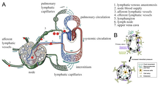
Figure 1.
Structure of the lymphatic system (LS): (A) adapted from [23,34] with permission. Lymphs enter the LS through the initial lymphatics (lymphatic capillaries), goes to larger lymphatic vessels, and is filtrated in lymph nodes. Then, it is collected in the trunks and ducts, which are the largest lymphatic vessels with respect to their diameter. Ducts open to the neck veins, which in turn open to the upper vena cava, and thus, lymphs return to the blood circulatory system. (B) Initial lymphatics (lymphatic capillaries): adapted from [35] with permission. Lymphs enter the lymphatic capillary through junctions between endothelial cells (ECs). These junctions are called primary (flap) valves because they prevent lymphs from leaving the lymphatic capillary. Capillaries are surrounded by the intermittent basement membrane. ECs connect to the surrounding extracellular matrix with anchoring filaments. Anchoring filaments prevent lymph capillaries from collapsing even in increased interstitial pressure (black arrow).
From the initial lymphatics, the lymph goes to the collectors, which have three layers of cells similar to blood vessels. There are secondary valves in these collectors which prevent the backward flow of lymphs. These valves consist of two or three leaflets located along with the flow (Figure 2A). Valves divide lymphatic vessels into functional parts, and the parts between adjacent valves are called lymphangions (Figure 2B). These lymphangions can produce active contractions. Contractions in the vessels with valves provide the unidirectional flow of lymph (Figure 2B), which is a characteristic property of lymph flow in the LS.
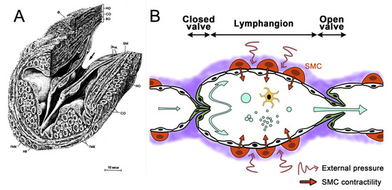
Figure 2.
Structure of the lymphatic vessels: (A) microscopic view of an open secondary valve in the lymphatic vessel. Reprinted from [36] with permission. The arrow indicates the direction of lymph flow. (B) A scheme of lymph flow in the lymphatic vessel with secondary valves: republished from [35] with permission. Secondary valves allow lymphs to flow in one direction and restricts flow in the backward direction. The part of the lymphatic vessel between adjacent valves is called a lymphangion. There are smooth muscle cells (SMCs) in the vessel wall which allow wall contractions. Lymphs flow in the vessel under active (intrinsic) contractions of the lymphatic vessel wall and under passive (extrinsic) contractions having external nature.
The network of lymphatic vessels is highly unstructured and contains many lymph nodes, and its hierarchical structure is shown in Figure 3. Numerous lymph nodes contained in the LS are lymphoid organs actively participating in the transport function of the LS [32].
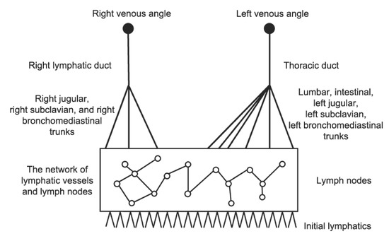
Figure 3.
A schematic representation of the LS. From the bottom to the top: the LS starts from the initial lymphatics and then the network of lymphatic vessels and lymph nodes, followed by trunks and ducts. The right lymphatic duct collects lymphs from the right part of the head and body and opens to the right venous angle. The thoracic duct collects lymphs from the left part of the head and body and both lower extremities. It opens to the left venous angle between neck veins. About 1/4 of lymphs goes to the right lymphatic duct, and 3/4 go to the thoracic duct [27,28].
It is believed now that lymph flows in the LS are because of the pressure gradient between the interstitial space and the upper vena cava and because of passive (extrinsic) contractions which are caused by the movements of muscle tissues, the diaphragm, and big blood vessels nearby and of active (intrinsic) contractions which are spontaneous contractions of lymphangions. The precise mechanism of active contractions is not yet well known [33]. One of the open questions is whether active contractions can produce enough force to drive the lymphs throughout the whole LS. The lymph flow cycle includes the entrance of lymphs into the initial lymphatics, the flow into lymphangions, and the flow into lymph nodes. The biomechanics of lymph flow in all these steps is not yet elucidated.
The majority of models of lymph flow in the lymphangion or series of lymphangions are based on the zero-dimensional (including lumped ones) [17,22,37,38] or one-dimensional (including quasi-one-dimensional ones) [18,39,40,41] approaches. “Lumped” models here are models based on electrical circuit theory, where the network of vessels is substituted with the circuit and where the voltage, current, and charge are equivalent to pressure, lymph flux, and mass, respectively [38,42,43]. Zero-dimensional models are models with no space distribution of velocity (flux) and pressure functions. Quasi-one-dimensional models are one-dimensional models in which the cross section may change. A three-dimensional formulation for lymph flow in the single lymphangion is considered in [44]. In the works [40,45], models of lymph flow in the whole LS are developed on the basis of zero-dimensional and quasi-one-dimensional approaches, respectively. The influence of valves and contractions on the flow distinguishes lymph flows from other physiological flows.
3. Flow in Lymphangions
We will describe lymph flow in this section using the quasi-one-dimensional approach [40] and other models when they are available. This approach is widely used to model systemic blood circulation [46,47] and, more recently, to model lymph flow in the lymphatic vessels [18,40,41]. In this approach, fluid flow is described by a system of hemodynamic equations which are derived from mass and momentum conservation (or from the Navier–Stocks equations [48]):
where is fluid velocity, is pressure, is cross sections area, is density, x is spatial coordinate, and t is time. The external force corresponds to viscous friction. Systems (1) and (2) are completed by the relation between the cross-sectional area s and pressure p. While this system is suitable to describe blood flow in arteries and veins, it cannot be used to describe lymph flow in lymphatic vessels without modifications because of the presence of valves and vessel wall contractions.
3.1. Influence of Valves
Secondary valves in lymphatic vessels prevent backward flow of lymphs and provide its unidirectional flow. Some investigations report that valves are included in the contraction of lymphangion [31]. Leaflets of valves can influence the flow. The models of secondary valves are usually limited by the absence of backward flow and sometimes by the resistance to the incoming flow.
Secondary valves can prolapse in a high adverse pressure gradient, and the presence of backward flow is one of the diagnostic criteria for lower limb lymphedema [49]. However, it is not known whether it is the reason for or a consequence of the disease [17]. Some models of valves include the possibility of prolapse.
There are several ways to represent the influence of valves on the lymph flow. One of them is to consider adjacent lymphangions as two segments connected with the bifurcation point. In this representation, the flow in each vessel is described by System (1, 2) and a closing relation. At the point of bifurcation, conditions on the pressure and flux are stated. Valves are taken into account in the flux condition at the bifurcation point, and the simplest model for their behavior is as follows [17,37]:
where is the lymph flux through the valve. Condition (3) restricts the backward lymph flow through the valve. Valve resistance to the incoming flow is considered in [37] on the basis of the data from [50].
A valve model in blood vessels for lumped and one-dimensional approximations is proposed in [51]. It is sufficiently simple and detailed to describe normal functioning of valves and their pathologies. This model is used in [39] to describe the valve influence on lymph flow. The equation for time-varying flux through valve has the following form:
where is pressure drop on the valve and where , , are functions of lymphatic inertia (proportional to ), Bernoulli resistance (proportional to ), and viscose resistance to flow (proportional to ), respectively.
In [22], the valve resistance changes in time, depending on pressure gradient in the lymphangion:
The transition from the maximal resistance to the minimal occurs when pressure difference before and after the valve reaches some threshold value is sufficient to open a valve. The second sigmoid describes the prolapse effect at the large adverse pressure gradient . In this formulation, resistance to backward flow has a large but limited value.
Another way to model the valve influence on lymph flow is to take it into account in the right-hand part of Equation (2). The valve provides some force influencing the flow in one direction but not in the opposite direction. This approach is used in [52] to model valve functioning in blood vessels. In [40], the valves in trunks and ducts are modelled by Equation (3). The valve influence in the smaller vessels is modelled by the following force in the right-hand side of the momentum equation:
where is a viscosity coefficient, considered as a function of velocity u having a sigmoidal form. This function characterizes friction force acting on flow in the backward direction. The sigmoidal form of this coefficient describes valve resistance to the upcoming flow. A similar approach was used in [41].
The choice of the valve model depends on the modeling task. If valve resistance to the flow is not important in the investigation, the simple boundary Condition (3) is sufficient. Formulas (4) and (5) allow for consideration of changing the valve resistance. Formula (6) is suitable for modeling multiple valves in big networks of lymphatic vessels [40]. It also allows for application of analytical methods to study lymph flow [53].
3.2. Influence of Contractions
Lymph flow in lymphatic vessels is influenced by active and passive contractions. Active contractions include a tonic part induced by intravascular pressure, and phase contractions are spontaneous and periodic (Figure 4). Active contractions are determined by lymphatic vessel wall properties and lymph chemical composition, while passive contractions occur due to some external reasons (e.g., muscle contractions or diaphragm movement). Biophysics of active contractions is not yet known. Many investigations consider the influence of different humoral factors on the amplitude, phase, and period of contractions, but a consistent theory does not exist. One more important question is about the coordination of contractions of adjacent lymphangions [17,22], since these data cannot be obtained from physiological experiments.
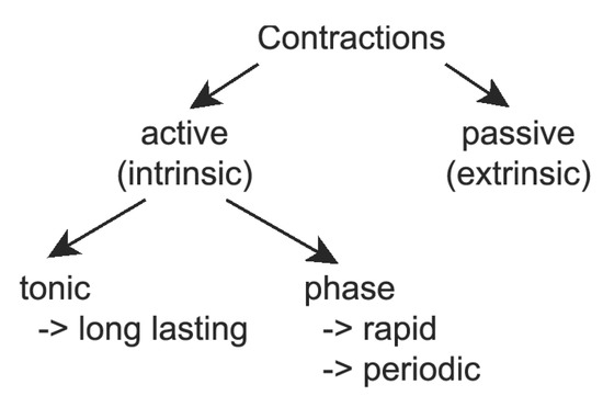
Figure 4.
Classification of lymphatic contractions: Active (intrinsic) contractions are caused by the vessel wall properties and the lymph formulae. Passive (extrinsic) contractions occur because of external factors. Active contractions can be divided into two parts: tonic response and phase contractions. The tonic response is a long-lasting variation of elastic properties of the vessel wall, and phase contractions are rapid and periodic. All these types of contractions can be modelled together [17] or separately [18,22,37,38,39,41,54,55]
In early works, contractions of lymphangions were modeled using the same approach as in the models of heart pumping with time-varying elasticity [17]:
where is dead volume (theoretical volume at zero pressure), is measured volume, and is transmural pressure. Therefore, passive and active contractions are taken into account in this model. This model was extended in [21], where contractions of two and more (up to four) lymphangions and their coordination were investigated. In this series of works, it was demonstrated that coordination of lymphangions minimally affects lymph flow. However, later investigations showed opposite results [22]. Both works are supported by physiological experiments, and, as discussed in [23], the reason for such a difference can be related to their design, in particular, the presence of valves can be essential.
Lymphangion contractions depend on the pressure gradient. Lymphangions contract if the pressure gradient is negative, and they act as passive conduits if the pressure gradient is positive [56]. Active contractions decrease flow under a positive pressure gradient [17,18]. Therefore, under these conditions, more effective drainage occurs without contractions. This result can bring a new understanding of lymphedema pathogenesis and treatment [17]. In particular, the reduction of pumping activity in some edemas can facilitate drainage of excessive fluid [17], while it is conventionally considered a pathogenesis of the disease.
Both components of active contractions are considered together in (7) [17,21]. In other models, they can be singled out in the pressure–area relationship closing Systems (1) and (2). They are considered below in Section 3.2.1 and Section 3.2.2, and passive contractions are considered in Section 3.2.3.
3.2.1. Modelling of Tonic Response
Tonic response determines how the vessel wall reacts to changing pressure inside the lumen. It is reported in [31] that elastic properties of lymphatic vessels are close to elastic properties of veins. More precise characteristic of lymph vessels is not yet determined.
In the quasi-one-dimensional approach, elastic properties of the vessel wall are usually taken into account in the third equation (also called state equation, tube law, or pressure–area relationship), which closes Systems (1) and (2) and describes dependence of the cross-sectional area on the intraluminal pressure:
Despite the existence of models concerning the cell structure of blood vessels, in the majority of investigations, empirical curves for the s–p relationship are used [57]. Similar representations are also used for all existing models of lymph flow on the basis of physiological experiments [18,22,37,39]. Despite the similarity of s–p curves for different pressure–area dependencies, mathematical solutions (in particular, the velocity of small perturbations) can differ significantly [57]. Let us consider implementations of tonic reactions in different models of lymph flow in lymphatic vessels.
The simplest pressure–area relationship with a linear dependence is used in [40]:
where is the minimum cross-sectional area at pressure and where is the coefficient characterising vessel elasticity. A nonlinear pressure–area relationship
is considered in [37]. Here, h is the lymphangion wall thickness, r is the time-dependent radius, is the resting radius, and E is the elasticity coefficient (Young’s module). Let us note that E in (10) has an opposite meaning compared to in (9): for larger E, the wall is more rigid. The tonic part is represented by the first term in brackets, while characterises phase contractions and is external passive pressure considered as a given function. In this formulation of the pressure–area relationship, the assumption of the thin vessel wall is imposed, i.e., wall thickness is supposed to be much smaller than lymphangion radius. A thick wall model is considered in [18]:
where is the transmural pressure (gradient between pressure inside of the vessel p and outside of the vessel ), and are the internal and external vessel radius respectively, is the radius variation caused by the pressure difference, and is the Poisson ratio. This formulation takes into account tube tension T resulting from longitudinal bending of the vessel and the damping term with coefficient . The damping term serves as a natural regularization for the explicit numerical scheme [18], helping to avoid the numerical instability observed in [45].
Another dependence was used in [22,55]:
where d is diameter, and and are some parameters. The exponent describes wall-stiffening with strain at positive transmural pressure, and the cubic term describes a progressively diminishing vessel compliance at negative transmural pressure. Two more refined forms of this relation are used by the same authors in [58]. A similar approach with more parameters is used in [39]. These parameters are determined by fitting the data from physiological experiments.
These models describe the elastic properties of lymphatic vessels. The parameters of Equation (9) can be directly measured from the physiological experiments (for s linearly depending on p). In (10) and (11), the additional model for Young’s module E is required [59]. Formula (12) closely represents the considered physiological experiment. However, as discussed in [57], the same s–p dependence can give different solutions depending on the exact s–p function. Since the level of uncertainty in parameter determination for lymph flow is very high, a more complex model does not necessarily work better. Therefore, the final choice of the model depends on the modelling task.
3.2.2. Phase Contractions
Phase contractions represent another type of active contraction. They provide lymph propagation in the low or inverse pressure gradient between the interstitial space and the upper vena cava. Lymphedema is associated with failure of these contractions. The precise mechanism of phase contractions is not known. It is generally recognized that phase contractions are periodic and have relaxation and contraction times and that the amplitude of contractions seems to depend on the lymph volume inside the lymphangion just before contraction (diastolic volume). During the contraction phase, the lymphangion diameter can decrease up to 40% compared to its relaxed state [60]. The lymphangion length also decreases in the contraction, but existing mathematical models do not take it into account because of its small contribution compared to the diameter decrease. Furthermore, in some investigations, valves are reported to actively participate in contraction activity [31]. In the existing mathematical models, the valves are considered as a passive mechanism restricting backward flow.
It is not known whether the contractions can produce sufficient force to provide lymph flow against the gravity force in low or inverse pressure gradients between the interstitial space and upper vena cava. The models of lymph flow in the series of contracting lymphangions and in the whole LS are developed to answer this question [17,22,37,38,61]. In [61], and this question is answered positively with the developed mathematical model (Section 4). However, the evaluated parameters exceed the physiological values reported in [31,62].
A 3D model for different types of phase contractions shows that lymph flow velocity can be approximated by Poiseuille profile [44].
Since the precise mechanism of phase contractions is not known, they are modelled by some periodic, usually trigonometric, function. For example, active contractions in [40] have the following form:
where is the phase part of active contractions to be added in Equation (9) and where A, , and a are the parameters of a contraction wave: amplitude, wave length, and wave velocity, respectively.
An analytical estimate of pumping efficiency in the vessel with valves described by (6) is presented in [53]. It is shown that increased frequency of contractions leads to an increase in output flux. The same is true for increased amplitude. These results are extended in [63], where lymph flow is considered in a detailed graph of the LS (Figure 5c).

Figure 5.
Examples of graphs of the LS: (a) The graph from [45], reprinted with permission. The graph contains 29 vessels including 297 lymphangions. The thoracic duct and its feeders are presented, and other parts have less detailed descriptions. (b) The graph from [65], reprinted with permission. The graph contains the majority of vessels presented in the anatomical model. The algorithm resolves mismatches from the anatomical model. Both ducts are presented. (c) The graph from [40]. The graph is spatially oriented, and thus calculations with respect to gravity force are possible [61]. The vessel network includes lymph nodes. Both ducts are presented. Also presented are zoom-ins on the region with the right and the left venous angles (top) and the region of the cisterna chyli (bottom).
The trigonometric function is also used in [37], taking into account the current volume of lymphs in lymphangions and relax time: if these thresholds are not reached, contraction does not happen; otherwise, contractions are modelled by sinus function with an amplitude depending on lymphangion volume. A threshold value for the pressure to activate a fixed impulse is also used in [38], and this is a rare example of the work where lymphangion contraction duality is taken into account. Namely, contractions under negative pressure gradient are triggered if internal pressure in the lymphangion rises above a pressure threshold value, and it acts as a simple conduit under positive pressure gradient. This model reproduces a pulsating flow, and it can be used for the construction of big vessel networks.
Both sinus waves, simple like in (13) and with time delay like in [37], are used in [18], showing good correlation with the results of physiological experiments. It is supposed that contraction waves in lymphatic vessel networks propagate in the backward direction, from downstream to upstream, and that this behavior should be more efficient. Backward propagation (against the valves) of contraction waves was recorded in these experiments [18]. Cosine waves are used in [22] for every segment in the chain of lymphangions, and their propagation is investigated. All models reproduce the pulsating nature of lymph flow.
Phase contractions with switching from the minimal to the maximal values
in tube law are modelled in [39]. Tonic , phase , and passive components are taken into account. Parameter is a state of contractions (designated by s in original work), which is a solution of the Electro-Fluid-Mechanical contraction (EFMC) model based on the FitzHugh–Nagumo model for action potentials [64], and is a function of a cross-sectional area similar to (12).
In this model, lymphatic vessel contraction activation is similar to heart pacemakers. According to this assumption, the FitzHugh–Nagumo model is modified and used to describe calcium-dependent contractions. Modeling results are in agreement with the experimental trends. To our knowledge, this is the first model of lymph flow dynamics where humoral factors influencing contractions are taken into account. The EFMC model opens new perspectives in the study of humoral influence on the lymph flow contractions in models of lymph flow dynamics.
3.2.3. Passive Contractions
Passive contractions are determined by external factors, such as muscle contractions, massage, diaphragm movement, etc. They are independent of the characteristics of lymphatic vessels and of the lymph chemical composition. Passive contractions are usually modeled as some function of pressure outside the vessel wall, and they are taken into account in (, see (11)). Consideration of passive contractions can be essential in models of systemic lymph flow, e.g., in [40], because big muscles, especially of the lower limbs, and diaphragm excursions can have a significant effect on lymph flow. In models of contractions in one lymphangion or a series of lymphangions, the function of external pressure corresponds to the pressure inside the bath containing lymph vessel segment in in vitro experiments.
4. Systemic Lymph Flow and Graphs of the LS
The LS is highly unstructured, and it has almost no tree structure (Figure 3). As a consequence, the construction of graphs of the LS is quite difficult. However, there are several works where this attempt was implemented.
A graph of the LS was constructed in [45] (Figure 5a), and to our knowledge, it is the first reported attempt to consider systemic lymph flow. This graph starts from the interstitial space in several organs and contains feeders of the thoracic duct and the thoracic duct itself, while the right lymphatic duct is not included. It has 296 lymphangions, some of which represent lymph nodes. Lymph flow in the lymphangions is described with the zero-dimensional model from [37], and the pressure equilibrium and flux conservation are imposed in the bifurcation points. This model gives a description of fluid exchange in the interstitial space with equations similar to those describing flow in lymphangions but including flux from the interstitial space instead of flux from the previous lymphangion. Flux in the interstitial space is given by a model of Starling law for fluid exchange, and it takes into account hydraulic and osmotic pressure. The model for tissue fluid exchange was further developed in [62] with the one-dimensional approach, including the influence of anchoring filaments and primary valves in the initial lymphatics. This systemic model shows the pulsating nature of lymph flow from the thoracic duct that is consistent with physiological observations. The parameters of the flow were in agreement with available physiological data.
The algorithm of automatic construction of a graph of the LS is suggested in [65]. The data from the Plastic Boy project [66] is used as a source of anatomical structure. These data are not suitable for calculations as-is, and the constructed algorithm turns this image into a consistent graph of the LS (Figure 5b). Structural analysis of the LS is provided, including the average degree of lymph nodes (how many vessels connected to the node). This algorithm can be applied to other anatomical models. The presence of a graph of the lymphatic system makes it possible to analyze the redistribution of lymph flow in the human lymphatic system in case of damage and/or difficulty in the outflow of lymphs from individual lymph nodes, which will allow for prediction of the effects of various injuries and changes in the organs of the human lymphatic system as well as for prediction of the best methods for correcting these problems.
One more graph of the LS is constructed in [40] (Figure 5c). It is anatomically adequate, spatially oriented, and topology consistent with a similar graph of the cardiovascular system [47]. The graph contains 271 collecting lymphatic vessels, thousands of lymphangions, and 161 lymph nodes. Groups of lymph nodes form the basis of the graph, and it contains 46 main groups [54]. Flow in the vessels is described by the quasi-one-dimensional equations including valve and active contraction influence, and the conditions of pressure equilibrium and mass conservation are imposed in the bifurcation points. The model of active pumping in this graph and its influence on the total flow are investigated without the influence of gravity force [63] and with influence of gravity force [61]. The increase in amplitude and frequency of phase contractions is shown to increase the output flux. Also, the elasticity and contractions of lymph nodes have a considerable effect on the output flux [63]. Therefore, the lymph nodes affect the transport function of the LS, and it is consistent with physiological observations [32]. The frequency of contractions, required to get output flux in physiology adequate intervals, is higher than reported in the physiological experiments [31,62]; however, in vivo parameters can also differ from them [15]. The consideration of passive contractions, which are not included in the model now, may allow for a reduction in the frequency. The results show that active contractions can produce enough force to make lymphs flow though the whole LS against the pressure gradient [61].
The approach used to construct a spatially oriented graph in [65] requires source images to contain information about both lymph nodes and lymphatic vessels. Another approach is used to create a graph in [40]. The basis of this graph is the regional groups of lymph nodes which connect according to the communication matrix filled in with data from [29]. This approach can be used to construct personalized graphs of the LS by extracting information about lymph nodes from MRI images and by connecting them with vessels using the communication matrix according to some anatomical source (i.e., [29]). The described concept could be the first step towards the creation of personalized graphs of the LS.
5. Lymph Drainage and Flow in Initial Lymphatics
The LS starts from the initial lymphatics (lymphatic capillaries, terminal lymphatics), where lymphs arrive from the interstitial space. Characteristic features of lymph drainage from the interstitial space are the influence of primary valves, which allow lymphs to enter the LS and which stop it from flowing out of the lymphatic capillaries, and the presence of anchoring filaments, which prevent initial lymphatics from collapse even in excess pressure in the interstitial fluid (Figure 1B).
In contrast to models of secondary valves, models of the primary valves often take into account the geometry of the valve—the curvature of the cell [67,68].
Flow into the initial lymphatics can be described by a system of ordinary differential equations, including flux and pressure balance and taking into account osmotic pressure according to Starling’s hypothesis [45]. Another model takes into account the primary valves influence given by Condition (3) and anchoring filaments with additional force in the pressure–area relationship similar to (10) [62]. This model describes pumping of income lymph flow in the LS due to fluctuations in the interstitial fluid pressure and to the suction effect of adjacent pumping lymphatic vessels.
Primary valve dynamics can also be described by the Stockes equation [67]:
where T is a unit tissue thickness, is pressure inside the fluid gap between the cells, Q is flux through the gap, and is dynamic viscosity. This equation must be solved simultaneously with the equation for cell deflection :
where is transendothelial pressure drop, is pressure inside the lumen, and E is Young’s module. Flux through the gap is given by the following expression:
where is flow velocity. Simulation results demonstrate primary valve dynamics for this model: the flux nonlinearly depends on pressure p with positive pressure gradient , and it equals 0 for negative pressure gradient.
This model was extended in [69], where a more precise description of flow around the overlapping endothelial cells is considered in the same geometry. The computational results correspond to the available physiological data.
The geometrical structure of the interstitial space with initial lymphatics and blood capillaries is considered in [68], and a mechanical model for primary valve dynamics concerning their curvatures is used to describe flow through the junctions between endothelial cells. As a result of this two-dimensional analysis, the formula for lymph flux per unit length q in terms of the pressure difference between blood and lymphatic capillaries was obtained:
where is the critical pressure needed to open a valve, is a dimensionless parameter that describes the effect of geometry on the fluid flux, k is permeability of intestitium, is viscosity of interstitial fluid, and is radius of the blood capillary. This model describes fluid exchange between blood and lymphatic capillaries through the interstitial space.
All considered models describe periodical entering of lymphs into the initial lymphatics. They provide more precise boundary conditions for models of flow in the lymphangions, and they can be used to describe lymph drainage in the investigations of lymphedema pathology.
6. The Structure and Function of the Lymph Node
Lymph nodes (LNs), which represent an important part of the lymphatic system, in addition to merging lymph flows, perform a number of functions related to the human immune system. This is due to the fact that they contain localized populations of cells that perform protective functions in the body. Thus, populations of T-lymphocytes are located in the so-called T-cell zone and B-lymphocytes are grouped in B-cell follicles, which are involved in the production of antibodies specific for the antigens entering the body. Dendritic and fibroblastic reticular cells are also present in the T-cell zone and are involved in all aspects of the functioning of lymph nodes. Figure 6 shows the key elements of the structure of the lymph node. These data are provided according to [70,71,72].
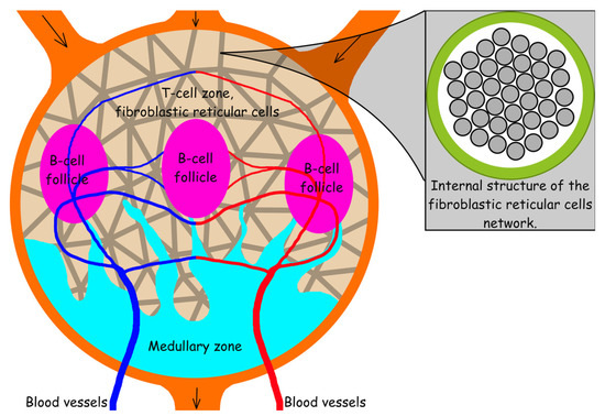
Figure 6.
Lymph node scheme illustrating its key elements: the scheme shows subcapsular sinus (orange), medullary zone (azure), B-cell follicles (purple), T-cell zone, a network of fibroblastic cells (gray lines against the background of the T-cell zone), afferent (introducing lymph) and efferent (excreting lymph), as well as blood vessels.
In the lymph node, T and B lymphocytes are in an inactive, naive state. The populations of these cells are regulated by fibroblastic reticular cells (FRC) secreting interleukin-7, which is a survival factor for naive lymphocytes [73]. The FRC network is also involved in maintaining the structural integrity of the entire organ through threads formed by polymerized collagen (Figure 6) secreted by fibroblastic reticular cells. The process of immune response in LNs begins with the helper T lymphocyte that has detected the antigen or with another activated antigen-presenting cell [74]. In this case, a cascade process occurs: T helper lymphocytes start activation of resting antigen-presenting cells, T effector lymphocytes and B-lymphocytes, and interleukin-2 is produced to increase the proliferative activity of T and B-lymphocytes [75]. Activated antigen-presenting cells (APC) fix onto the FRC network for a period of about 6 hours with the possibility of subsequent reactivation. After that, APCs begin to express interferon-. Under the influence of interferon-, naive T effector lymphocytes specialize according to the components of the antigen, presented by the antigen-presenting cells’ major histocompatibility complex class I, II (MHC class I, II) [76]. At the same time, the FRC network is actively involved in stimulating immune response, producing chemokines CCL19 and CCL21. According to existing data, the lymphocytes interacting with these chemokines exhibit increased motor activity. This effect does not improve immune response alone, but in synergy with the chemotaxis effect used by cells to search for foci of infection, chemokines shortened the time from activation to interaction with the target. Activated B-lymphocytes can also activate resting cells, but their main function is the production of antibodies specific for the target antigen [74]. At the same time, activated T effector lymphocytes search for and destroy cells expressing signals characteristic of the desired antigen. T effector lymphocytes mainly destroy body cells infected with intracellular parasites (viruses or bacteria). Macrophages are also involved in the process of the immune response, destroying free viruses and bacteria. After activation in the lymph nodes, cells of the immune system move into tissues in which antigens are present to fulfill functions of the immune response. In connection with such a heterogeneous structure of the lymph nodes, it becomes extremely important to understand how the lymph flows into the node are distributed ([77,78]). The size of particles that can enter different zones of the lymph node is limited [77]. Thus, it turns out that huge viruses and bacteria cannot penetrate into the T-cell zone through the walls of the FRC network due to too large sizes. Therefore, they get there either through blood vessels or inside the cells that came from outside the lymph node. It should be noted that the detection of antigens is difficult not only because of the limited methods of their entry into the T-cell zone. About 93% of lymphs generally passes through the subcapsular sinus of the LN. This is shown, inter alia, in [78]. It should also be taken into account that part of the lymph from the lymph node enters the blood vessels system inside LNs.
Due to the complexity of the processes occurring in the lymph nodes and the heterogeneity of the lymph nodes, it becomes necessary to be able to form various configurations of the lymph nodes to simulate the processes of cell interactions, fluid flow, and collagen coagulation. Since it is expensive and time-consuming to restore structures using layer-by-layer scanning, an important area of research is the development of algorithmic methods for constructing lymph nodes. Algorithms were developed, and 3D models of the components of the lymph node were built in [79,80]. Three-dimensional models of key elements of LNs in a voxel format were created with further conversion to a solid-state 3D model: the shell of the lymph node, trabecular and medullary sinuses, B-cell follicles, and a network of fibroblastic reticular cells.
Separately, algorithms were developed to build a 3D model of a network of fibroblastic reticular cells [80]. It appears that a highly damaged network (up to 50%) can still support lymph flow. This is important for the case of HIV infection where the structure of the fibroblastic reticular cells as well as the ducts formed by them are gradually destroyed. Damage of the network significantly affects not only the ability of the T-cell zone of the lymph node to pass lymphs but also the homeostasis of cell populations and the immune response to HIV in general [80,81].
7. Conclusions and Perspectives
The main goal of investigations of lymph flow is to understand the underlying mechanisms in order to propose effective therapeutic techniques. In the 90s, the specific lymphatic factor (VEGF–C) was discovered, and it led to the explosive investigation of LS [82]. The mechanisms of lymph flow are more clear now, but there are still many open questions.
Mathematical modeling is used with in vitro experiments to get more data, to check the hypothesis about lymph flow, and to construct new experiments. In [17,21], the authors established conditions for pumping and conduit acting. In negative pressure difference, the lymphangion acts as an active pump, and in positive pressure, it acts as a simple conduit. Moreover, in large positive pressure gradients, active contractions are shown to inhibit lymph flow. This result is supported by a physiological experiment [18,56]. The meaning of this result in the application to lymphedema pathogenesis and treatment is discussed in [17]. For some edemas, the inhibition of lymphangion pumping may have a positive effect.
Pathogenesis and treatment of lymphedema are one of the most important applications of models of lymph flow in lymphatic vessels. Direct models of lymph flow in lymphatic vessels are not the only way to address edema pathology: in [83], lymph filtration through the extremity was considered with diffusion equations instead of considering flow in separate vessels, and some clinical recommendations (for using of bandages) were proposed.
Another important goal of lymph flow modelling is the investigation of drug distribution in the LS and various tissues and organs. Insufficient lymphatic circulation is one of possible reasons for ineffective drug therapy, and such a model for systemic circulation can find its applications not only for lymphedema treatment but also for other drug-delivery tasks. Lymph drainage from the interstitial fluid and sorption effect of the secondary lymphatic circulation (vessels with contractions and secondary valves) are essential for understanding the mechanisms of more efficient drainage in the cases of different pathologies. The proposed concept for construction of personalized graphs of the LS could be the first step towards achieving a personalized model of human LS. It opens new perspectives in these investigations.
Lymph flow in the lymph node may influence the immune response occurring in them. Modeling the processes of cellular interactions in the lymph nodes as well as the processes of transfer between nodes through the lymphatic system are critical for understanding the processes that occur in HIV-infected people. It gives an opportunity to develop the best strategies for drug therapy, to analyze the effectiveness of existing methods, and to find key relationships in complex immune response processes. The human immune system depends on many populations of cells represented in the T-cell zone of the lymph nodes: T-lymphocytes (helpers and effectors); B-lymphocytes, which produce antibodies when pathogens enter the body; macrophages; and antigen-presenting cells. Certain cell populations, such as fibroblast reticular cells, are involved in maintaining the homeostasis of naive lymphocyte populations, and the whole lymphatic system provides a reserve of bandwidth for the fluid circulation in the body and acts as another filter for intercellular fluid collected by lymphatic capillaries from tissues.
There are still many open questions in lymph flow mechanics, but close cooperation between physiologists and mathematicians will help understand it better.
Author Contributions
Writing—original draft preparation, A.M. and R.S. All authors have read and agreed to the published version of the manuscript.
Funding
This work is supported by the Ministry of Science and Higher Education of the Russian Federation: agreement no. 075-03-2020-223/3 (FSSF-2020-0018).
Conflicts of Interest
The authors declare no conflict of interest.
References
- Choi, I.; Lee, S.; Hong, Y.K. The New Era of the Lymphatic System: No Longer Secondary to the Blood Vascular System. Cold Spring Harb. Perspect. Med. 2012, 2, 23. [Google Scholar] [CrossRef] [PubMed]
- Filchenkov, A.A. Lymphangiogenesis and metastasis of tumors. Creat. Surg. Oncol. 2010, No. 3. 80–90. (In Russian) [Google Scholar]
- Itkin, M.; McCormack, F.; Dori, Y. Diagnosis and Treatment of Lymphatic Plastic Bronchitis in Adults Using Advanced Lymphatic Imaging and Percutaneous Embolization. Ann. Am. Thorac. Soc. 2016, 13, 1689–1696. [Google Scholar] [CrossRef] [PubMed]
- Pamarthi, V.; Pabon-Ramos, W.M.; Marnell, V.; Hurwitz, L.M. MRI of the Central Lymphatic System: Indications, Imaging Technique, and Pre-Procedural Planning. Top. Magn. Reson. Imaging 2017, 26, 175–180. [Google Scholar] [CrossRef] [PubMed]
- Louveau, A.; Smirnov, I.; Keyes, T.J.; Eccles, J.D.; Rouhani, S.J.; Peske, J.D.; Derecki, N.C.; Castle, D.; Mandell, J.W.; Lee, K.S.; et al. Structural and functional features of central nervous system lymphatic vessels. Nature 2015, 523, 337–341. [Google Scholar] [CrossRef] [PubMed]
- Aspelund, A.; Antila, S.; Proulx, S.T.; Karlsen, T.V.; Karaman, S.; Detmar, M.; Wiig, H.; Alitalo, K. A dural lymphatic vascular system that drains brain interstitial fluid and macromolecules. J. Exp. Med. 2015, 212, 991–999. [Google Scholar] [CrossRef] [PubMed]
- Nikolenko, V.N.; Oganesyan, M.V.; Yakhno, N.N.; Orlov, E.A.; Porubayeva, E.E.; Popova, E.Y. The brain’ sglymphatic system: Physiological anatomy and clinical perspectives. Neurol. Neuropsychiatry Psychosom. 2018, 10, 94–100. [Google Scholar] [CrossRef]
- Munn, L.L.; Padera, T.P. Imaging the lymphatic system. Microvasc. Res. 2014, 96, 55–63. [Google Scholar] [CrossRef]
- Sharma, R.; Wendt, J.A.; Rasmussen, J.C.; Adams, K.E.; Marshall, M.V.; Sevick-Muraca, E.M. New Horizons for Imaging Lymphatic Function. Ann. N. Y. Acad. Sci. 2008, 1131, 13–36. [Google Scholar] [CrossRef]
- Liu, N.F.; Lu, Q.; Jiang, Z.H.; Wang, C.G.; Zhou, J.G. Anatomic and functional evaluation of the lymphatics and lymph nodes in diagnosis of lymphatic circulation disorders with contrast magnetic resonance lymphangiography. J. Vasc. Surg. 2009, 49, 980–987. [Google Scholar] [CrossRef]
- Sevick-Muraca, E.M.; Sharma, R.; Rasmussen, J.C.; Marshall, M.V.; Wendt, J.A.; Pham, H.Q.; Bonefas, E.; Houston, J.P.; Sampath, L.; Adams, K.E.; et al. Imaging of Lymph Flow in Breast Cancer Patients after Microdose Administration of a Near-Infrared Fluorophore: Feasibility Study. Radiology 2008, 246, 734–741. [Google Scholar] [CrossRef] [PubMed]
- Kwon, S.; Sevick-Muraca, E.M. Noninvasive Quantitative Imaging of Lymph Function in Mice. Lymphat. Res. Biol. 2007, 5, 219–232. [Google Scholar] [CrossRef] [PubMed]
- Sharma, R.; Wang, W.; Rasmussen, J.C.; Joshi, A.; Houston, J.P.; Adams, K.E.; Cameron, A.; Ke, S.; Kwon, S.; Mawad, M.E.; et al. Quantitative imaging of lymph function. Am. J. Physiol. Heart Circ. Physiol. 2007, 292, H3109–H3118. [Google Scholar] [CrossRef] [PubMed]
- Dixon, J.B.; Zawieja, D.C.; Gashev, A.A.; Cote, G.L. Measuring microlymphatic flow using fast video microscopy. J. Biomed. Opt. 2005, 10, 064016. [Google Scholar] [CrossRef]
- Zawieja, S.D.; Castorena-Gonzalez, J.A.; Dixon, B.; Davis, M.J. Experimental Models Used to Assess Lymphatic Contractile Function. Lymphat. Res. Biol. 2017, 15, 331–342. [Google Scholar] [CrossRef]
- Blatter, C.; Meijer, E.F.J.; Nam, A.S.; Jones, D.; Bouma, B.E.; Padera, T.P.; Vakoc, B.J. In vivo label-free measurement of lymph flow velocity and volumetric flow rates using Doppler optical coherence tomography. Sci. Rep. 2016, 6. [Google Scholar] [CrossRef]
- Quick, C.M.; Venugopal, A.M.; Gashev, A.A.; Zawieja, D.C.; Stewart, R.H. Intrinsic pump-conduit behavior of lymphangions. Am. J. Physiol. Regul. Integr. Comp. Physiol. 2007, 292, R1510–R1518. [Google Scholar] [CrossRef]
- Macdonald, A.J.; Arkill, K.P.; Tabor, G.R.; McHale, N.G.; Winlove, C.P. Modeling flow in collecting lymphatic vessels: One-dimensional flow through a series of contractile elements. Am. J. Physiol. Heart Circ. Physiol. 2008, 295, H305–H313. [Google Scholar] [CrossRef][Green Version]
- Lobov, G.I.; Pan’kova, M.N.; Abdreshov, S.N. Phase and tonic contractions of lymphatic vessels and nodes under the action of atrial natriuretic peptide. Reg. Blood Circ. Microcirc. 2015, 14, 72–77. (In Russian) [Google Scholar] [CrossRef]
- Ohhashi, T.; Mizuno, R.; Ikomi, F.; Kawai, Y. Current topics of physiology and pharmacology in the lymphatic system. Pharmacol. Ther. 2005, 105, 165–188. [Google Scholar] [CrossRef]
- Venugopal, A.M.; Stewart, R.H.; Laine, G.A.; Dongaonkar, R.M.; Quick, C.M. Lymphangion coordination minimally affects mean flow in lymphatic vessels. Am. J. Physiol. Heart Circ. Physiol. 2007, 293, H1183–H1189. [Google Scholar] [CrossRef]
- Bertram, C.D.; Macaskill, C.; Moore, J.E. Simulation of a Chain of Collapsible Contracting Lymphangions With Progressive Valve Closure. J. Biomech. Eng. 2010, 133. [Google Scholar] [CrossRef] [PubMed]
- Margaris, K.N.; Black, R.A. Modelling the lymphatic system: Challenges and opportunities. J. R. Soc. Interface 2012, 9, 601–612. [Google Scholar] [CrossRef] [PubMed]
- Roose, T.; Tabor, G. Multiscale Modelling of Lymphatic Drainage. In Multiscale Computer Modeling in Biomechanics and Biomedical Engineering; Springer: Berlin/Heidelberg, Germany, 2012; pp. 149–176. [Google Scholar] [CrossRef]
- Guyton, A.C.; Hall, J.E. Textbook of Medical Physiology; Logosphere: Moscow, Russia, 2008; p. 1296. (In Russian) [Google Scholar]
- Schmidt, R.; Thews, G. Human Physiology; Mir: Moscow, Russia, 2005; Volume 2, p. 314. (In Russian) [Google Scholar]
- McKinley, M.; O’Loughlin, V.D. Human Anatomy; McGraw-Hill: New York, NY, USA, 2012; p. 966. [Google Scholar]
- Moore, J.E.; Bertram, C.D. Lymphatic System Flows. Ann. Rev. Fluid Mech. 2018, 50, 459–482. [Google Scholar] [CrossRef]
- Borzyak, E.; Bocharov, V.; Sapin, M. Human Anatomy; Medicine: Moscow, Russia, 1993; Volume 2, p. 560. (In Russian) [Google Scholar]
- Sinelnikov, R.; Sinelnikov, Y. Atlas of Human Anatomy. The Doctrine of the Vessels; Medicine: Moscow, Russia, 1996; Volume 3, p. 219. (In Russian) [Google Scholar]
- Petrenko, V.M. Functional Morphology of Lymphatic Vessels; DEAN: Saint Petersburg, Russia, 2008; p. 400. (In Russian) [Google Scholar]
- Lobov, G.I.; Pan’kova, M.N. Lymph transport in lymphatic nodes: Mechanisms of regulation. Ross. Fiziol. Zhurnal Im. I.M. Sechenova 2013, 98, 1350–1361. (In Russian) [Google Scholar]
- Zawieja, D.C. Contractile Physiology of Lymphatics. Lymphat. Res. Biol. 2009, 7, 87–96. [Google Scholar] [CrossRef] [PubMed]
- Quéré, I. Description anatomique et histologique, physiologie du système lymphatique. La Presse Médicale 2010, 39, 1269–1278. [Google Scholar] [CrossRef] [PubMed]
- Schulte-Merker, S.; Sabine, A.; Petrova, T.V. Lymphatic vascular morphogenesis in development, physiology, and disease. J. Cell Biol. 2011, 193, 607–618. [Google Scholar] [CrossRef] [PubMed]
- Krstic, R. Human Microscopic Anatomy: An Atlas for Students of Medicine and Biology; World and Education: Moscow, Russia, 2010; p. 608. (In Russian) [Google Scholar]
- Reddy, N.P.; Krouskop, T.A.; Paul, H. Newell, j. Biomechanics of a Lymphatic Vessel. J. Vasc. Res. 1975, 12, 261–278. [Google Scholar] [CrossRef]
- Gajani, G.S.; Boschetti, F.; Negrini, D.; Martellaccio, R.; Milanese, G.; Bizzarri, F.; Brambilla, A. A lumped model of lymphatic systems suitable for large scale simulations. In Proceedings of the 2015 European Conference on Circuit Theory and Design (ECCTD), Trondheim, Norway, 24–26 August 2015. [Google Scholar] [CrossRef]
- Contarino, C.; Toro, E.F. A one-dimensional mathematical model of collecting lymphatics coupled with an electro-fluid-mechanical contraction model and valve dynamics. Biomech. Model. Mechanobiol. 2018, 17, 1687–1714. [Google Scholar] [CrossRef]
- Mozokhina, A.S.; Mukhin, S.I. Pressure Gradient Influence on Global Lymph Flow. In Trends in Biomathematics: Modeling, Optimization and Computational Problems; Springer International Publishing: Berlin/Heidelberg, Germany, 2018; pp. 325–334. [Google Scholar] [CrossRef]
- Tretyakova, R.M.; Lobov, G.I.; Bocharov, G.A. Modelling lymph flow in the lymphatic system: From 0D to 1D spatial resolution. Math. Model. Nat. Phenom. 2018, 13, 45. [Google Scholar] [CrossRef]
- Milišić, V.; Quarteroni, A. Analysis of lumped parameter models for blood flow simulations and their relation with 1D models. ESAIM Math. Model. Numer. Anal. 2004, 38, 613–632. [Google Scholar] [CrossRef]
- Kokalari, I.; Karaja, T.; Guerrisi, M. Review on lumped parameter method for modeling the blood flow in systemic arteries. J. Biomed. Sci. Eng. 2013, 6, 92–99. [Google Scholar] [CrossRef]
- Rahbar, E.; Moore, J.E.J. A model of a radially expanding and contracting lymphangion. J. Biomech. 2011, 44, 1001–1007. [Google Scholar] [CrossRef]
- Reddy, N.P.; Krouskop, T.A.; Newell, P.H. A computer model of the lymphatic system. Comput. Biol. Med. 1977, 7, 181–197. [Google Scholar] [CrossRef]
- Sherwin, S.; Franke, V.; Peiró, J.; Parker, K. One-dimensional modelling of a vascular network in space-time variables. J. Eng. Math. 2003, 47, 217–250. [Google Scholar] [CrossRef]
- Bunicheva, A.Y.; Mukhin, S.I.; Sosnin, N.V.; Khrulenko, A.B. Mathematical modeling of quasi-one-dimensional hemodynamics. Comput. Math. Math. Phys. 2015, 55, 1381–1392. [Google Scholar] [CrossRef]
- Barnard, A.L.; Hunt, W.; Timlake, W.; Varley, E. A Theory of Fluid Flow in Compliant Tubes. Biophys. J. 1966, 6, 717–724. [Google Scholar] [CrossRef]
- Phionik, O. Clinical and Morpho-Functional Bases for Diagnostic and Treatment of Lymphedema of Low Limbs. Ph.D. Thesis, St Petersburg University, Saint Petersburg, Russia, 2008. (In Russian). [Google Scholar]
- Zweifach, B.W. Micropressure measurements in the terminal lymphatics. Bibl. Anat. 1973, 12, 361–365. [Google Scholar]
- Mynard, J.P.; Davidson, M.R.; Penny, D.J.; Smolich, J.J. A simple, versatile valve model for use in lumped parameter and one-dimensional cardiovascular models. Int. J. Numer. Methods Biomed. Eng. 2011, 28, 626–641. [Google Scholar] [CrossRef]
- Simakov, S.; Gamilov, T.; Soe, Y.N. Computational study of blood flow in lower extremities under intense physical load. Russ. J. Numer. Anal. Math. Model. 2013, 28. [Google Scholar] [CrossRef]
- Mozokhina, A.S.; Mukhin, S.I. Quasi-One-Dimensional Flow of a Fluid with Anisotropic Viscosity in a Pulsating Vessel. Differ. Equ. 2018, 54, 938–944. [Google Scholar] [CrossRef]
- Mozokhina, A.; Mukhin, S.; Koshelev, V. Quasi-Onedimensional Approach for Modeling the Lymph Flow in the Lymphatic System; MAKS Press: Moscow, Russia, 2017; p. 20. (In Russian) [Google Scholar]
- Jamalian, S.; Bertram, C.D.; Richardson, W.J.; Moore, J.E. Parameter sensitivity analysis of a lumped-parameter model of a chain of lymphangions in series. Am. J. Physiol. Heart Circ. Physiol. 2013, 305, H1709–H1717. [Google Scholar] [CrossRef] [PubMed]
- Quick, C.M.; Ngo, B.L.; Venugopal, A.M.; Stewart, R.H. Lymphatic pump-conduit duality: Contraction of postnodal lymphatic vessels inhibits passive flow. Am. J. Physiol. Heart Circ. Physiol. 2009, 296, H662–H668. [Google Scholar] [CrossRef] [PubMed]
- Vassilevski, Y.V.; Salamatova, V.Y.; Simakov, S.S. On the elasticity of blood vessels in one-dimensional problems of hemodynamics. Comput. Math. Math. Phys. 2015, 55, 1567–1578. [Google Scholar] [CrossRef]
- Bertram, C.; Macaskill, C.; Moore, J. Pump function curve shape for a model lymphatic vessel. Med. Eng. Phys. 2016, 38, 656–663. [Google Scholar] [CrossRef][Green Version]
- Absi, R. Revisiting the pressure-area relation for the flow in elastic tubes: Application to arterial vessels. Ser. Biomech. 2018, 32, 47–59. [Google Scholar]
- Macdonald, A.J. The Computational Modelling of Collecting Lymphatic Vessels. Ph.D. Thesis, University of Exeter, England, UK, 2008. [Google Scholar]
- Mozokhina, A.; Lobov, G. Simulation of lymph flow with consideration of natural gravity force influence. ITM Web Conf. 2020, 31, 01003. [Google Scholar] [CrossRef][Green Version]
- Reddy, N.; Patel, K. A mathematical model of flow through the terminal lymphatics. Med. Eng. Phys. 1995, 17, 134–140. [Google Scholar] [CrossRef]
- Mozokhina, A.S.; Mukhin, S.I.; Lobov, G.I. Pump efficiency of lymphatic vessels: Numeric estimation. Russ. J. Numer. Anal. Math. Model. 2019, 34, 261–268. [Google Scholar] [CrossRef]
- Franzone, P.C.; Pavarino, L.F.; Scacchi, S. Mathematical Cardiac Electrophysiology; Springer International Publishing: Berlin/Heidelberg, Germany, 2014. [Google Scholar] [CrossRef]
- Tretyakova, R.; Savinkov, R.; Lobov, G.; Bocharov, G. Developing Computational Geometry and Network Graph Models of Human Lymphatic System. Computation 2017, 6, 1. [Google Scholar] [CrossRef]
- Plasticboy. Plasticboy Pictures 2009 CC. Available online: http://www.plasticboy.co.uk/store/Human_Lymphatic_System_no_textures.html (accessed on 21 April 2020).
- Mendoza, E.; Schmid-Schonbein, G.W. A Model for Mechanics of Primary Lymphatic Valves. J. Biomech. Eng. 2003, 125, 407–414. [Google Scholar] [CrossRef] [PubMed]
- Heppell, C.; Richardson, G.; Roose, T. A Model for Fluid Drainage by the Lymphatic System. Bull. Math. Biol. 2012, 75, 49–81. [Google Scholar] [CrossRef] [PubMed]
- Galie, P.; Spilker, R.L. A Two-Dimensional Computational Model of Lymph Transport Across Primary Lymphatic Valves. J. Biomech. Eng. 2009, 131. [Google Scholar] [CrossRef]
- Novkovic, M.; Onder, L.; Cheng, H.W.; Bocharov, G.; Ludewig, B. Integrative Computational Modeling of the Lymph Node Stromal Cell Landscape. Front. Immunol. 2018, 9. [Google Scholar] [CrossRef]
- Mueller, S.N.; Germain, R.N. Stromal cell contributions to the homeostasis and functionality of the immune system. Nat. Rev. Immunol. 2009, 9, 618–629. [Google Scholar] [CrossRef]
- Turley, S.J.; Fletcher, A.L.; Elpek, K.G. The stromal and haematopoietic antigen-presenting cells that reside in secondary lymphoid organs. Nat. Rev. Immunol. 2010, 10, 813–825. [Google Scholar] [CrossRef]
- Link, A.; Vogt, T.K.; Favre, S.; Britschgi, M.R.; Acha-Orbea, H.; Hinz, B.; Cyster, J.G.; Luther, S.A. Fibroblastic reticular cells in lymph nodes regulate the homeostasis of naive T cells. Nat. Immunol. 2007, 8, 1255–1265. [Google Scholar] [CrossRef]
- Alberts, B.; Johnson, A.; Lewis, J.; Raff, M.; Roberts, K.; Walter, P. Molecular Biology of the Cell, 4th ed.; Garland Science: New York, NY, USA, 2002. [Google Scholar]
- Bachmann, M.F.; Oxenius, A. Interleukin 2: From immunostimulation to immunoregulation and back again. EMBO Rep. 2007, 8, 1142–1148. [Google Scholar] [CrossRef]
- Hochrein, H.; Shortman, K.; Vremec, D.; Scott, B.; Hertzog, P.; O’Keeffe, M. Differential Production of IL-12, IFN-α, and IFN-γ by Mouse Dendritic Cell Subsets. J. Immunol. 2001, 166, 5448–5455. [Google Scholar] [CrossRef]
- Cooper, L.J.; Heppell, J.P.; Clough, G.F.; Ganapathisubramani, B.; Roose, T. An Image-Based Model of Fluid Flow Through Lymph Nodes. Bull. Math. Biol. 2015, 78, 52–71. [Google Scholar] [CrossRef] [PubMed]
- Jafarnejad, M.; Woodruff, M.C.; Zawieja, D.C.; Carroll, M.C.; Moore, J. Modeling Lymph Flow and Fluid Exchange with Blood Vessels in Lymph Nodes. Lymphat. Res. Biol. 2015, 13, 234–247. [Google Scholar] [CrossRef]
- Kislitsyn, A.; Savinkov, R.; Novkovic, M.; Onder, L.; Bocharov, G. Computational Approach to 3D Modeling of the Lymph Node Geometry. Computation 2015, 3, 222–234. [Google Scholar] [CrossRef]
- Savinkov, R.; Kislitsyn, A.; Watson, D.J.; van Loon, R.; Sazonov, I.; Novkovic, M.; Onder, L.; Bocharov, G. Data-driven modelling of the FRC network for studying the fluid flow in the conduit system. Eng. Appl. Artif. Intell. 2017, 62, 341–349. [Google Scholar] [CrossRef]
- Donovan, G.M.; Lythe, G. T cell and reticular network co-dependence in HIV infection. J. Theor. Biol. 2016, 395, 211–220. [Google Scholar] [CrossRef] [PubMed]
- Pepper, M.S.; Tille, J.C.; Nisato, R.; Skobe, M. Lymphangiogenesis and tumor metastasis. Cell Tissue Res. 2003, 314, 167–177. [Google Scholar] [CrossRef] [PubMed]
- Eymard, N.; Volpert, V.; Quere, I.; Lajoinie, A.; Nony, P.; Cornu, C. A 2D Computational Model of Lymphedema and of its Management with Compression Device. Math. Model. Nat. Phenom. 2017, 12, 180–195. [Google Scholar] [CrossRef]
© 2020 by the authors. Licensee MDPI, Basel, Switzerland. This article is an open access article distributed under the terms and conditions of the Creative Commons Attribution (CC BY) license (http://creativecommons.org/licenses/by/4.0/).