The Calculation of the Density and Distribution Functions of Strictly Stable Laws

Abstract

Integral representations for the probability density and distribution function of a strictly stable law with the characteristic function in the Zolotarev’s “C” parametrization were obtained in the paper. The obtained integral representations express the probability density and distribution function of standard strictly stable laws through a definite integral. Using the methods of numerical integration, the obtained integral representations allow us to calculate the probability density and distribution function of a strictly stable law for a wide range of admissible values of parameters $(\alpha ,\theta )$. A number of cases were given when numerical algorithms had difficulty in calculating the density. Formulas were given to calculate the density and distribution function with an arbitrary value of the scale parameter $\lambda$.

1. Introduction

The problem of calculating the density of a strictly stable law with the characteristic function

$$\tilde{g}(t,\alpha ,\theta ,\lambda )=exp\{-\lambda {\left|t\right|}^{\alpha }exp\{-i\frac{\pi }{2}\alpha \theta \mathrm{sign}t\}\},t\in \mathbf{R},$$

(1)

where $0<\alpha ⩽2,\left|\theta \right|⩽min(1,2/\alpha -1),\lambda >0$ is considered in the paper. One of the reasons why it became necessary to calculate the density of a strictly stable law with this characteristic function is the need to calculate the density of a fractionally stable law which is defined by the expression

$$q(x,\alpha ,\nu ,\theta )={\int }_0^{\infty }g(x{y}^{\nu /\alpha },\alpha ,\theta )g(y,\nu ,1)y^{\nu /\alpha }dy.$$

(2)

Here, $g(x,\alpha ,\theta )$ and $g(y,\nu ,1)$ are the densities of strictly stable and one-sided strictly stable laws with the characteristic function in Equation (1) and parameter $\lambda =1$. For the first time, the density in Equation (2) was obtained in the article [1]. The density in Equation (2) got its name in the work [2], since the random variable $Z(\alpha ,\nu ,\theta )$ distributed by this law is defined by the ratio $Z(\alpha ,\nu ,\theta )=Y(\alpha ,\theta ){\left[V(\nu ,1)\right]}^{-\nu /\alpha }$. Here the random variables $Y(\alpha ,\theta )$ and $V(\nu ,1)$ are distributed by the laws $g(x,\alpha ,\theta )$ and $g(y,\nu ,1)$, respectively.

The density Equation (2) appears as a limit distribution with the following random walk scheme. Let the particle be at the origin $x=0$ at the initial time $t=0$ and it stays at this point during random time $T_1$. Then, it instantly moves with an equal probability to the right or left at random distance $X_1$ and it stays at rest again random time $T_2$. Then, the whole process is repeated in the same way. Values $X_i,i=1,2,\dots$ are independent identically distributed random variables belonging to the domain of normal attraction of a strictly stable law $g(t,\alpha ,\theta )$ with the characteristic function in Equation (1). Values $T_i,i=1,2,\dots$ are independent both between themselves and of the sequence $\left\{X_i\right\}$ by identically distributed random variables belonging to the domain of normal attraction of a strictly stable law $g(t,\nu ,1)$ with the characteristic function in Equation (1) and $0<\nu ⩽1$. We will form the sum of these random variables $S\left(\tau \right)={\sum }_{i=1}^{N\left(\tau \right)}{X}_i,\tau >0$, where $N\left(\tau \right)$ is the counting process: $N\left(\tau \right)=max\left\{n:{\sum }_{i=1}^n{T}_i⩽\tau \right\}$. The physical interpretation of the sum $S\left(\tau \right)$ is the coordinate of particle x at time $\tau$. In the works [1,2] it has been shown that the asymptotic (at $\tau \to \infty$) distribution of the sum $S\left(\tau \right)$ is described by the distribution Equation (2).

The described random walk scheme is called Continuous Time Random Walk (CTRW). For the first time it was considered in the work [3]. Later, it was described in the works [4,5,6]. For more detailed familiarity with this model one can look through the overviews [7,8]. In the work [1] it has been shown that the asymptotic (at $t\to \infty$) distribution of the CTRW process is described with the distribution (2). In the work [9], it has been shown that the CTRW process in large time asymptotics is described with the fractional-differential equation of diffusion. The solution of this equation is expressed through fractional-stable distributions in Equation (2). This is one of the factors determining the interest in studying the class of the fractional-stable laws.

Another factor is the appearance of these distributions in various processes occurring in a plasma [10,11] or in biology processes [12,13,14]. In particular, the fractional-stable distributions were used to describe a distribution of the gene expression in cells of tissues of various organisms in the following papers [12,13,14]. It is known that the distribution of the gene expression is described by laws with the power decrease in the density [15,16,17]. Since the density in Equation (2) decreases as $x^{-\alpha -1}$ at $x\to \infty$, therefore this class of distributions was used to describe the gene expression distribution. In the articles [12,13] the fractional-stable distributions were used to describe the gene expression obtained with the microarray technology. In the paper [14], these distributions were used to describe the results obtained with the Next Generation Sequence technology. In the papers [12,13,14] the Monte Carlo method was used to calculate the density $q(x,\alpha ,\nu ,\theta )$. To estimate the parameters $(\alpha ,\nu ,\theta )$ of the fractional-stable law a method described in [18] was used which is also based on the Monte Carlo method. However, to construct more effective estimators of the parameters $(\alpha ,\nu ,\theta )$, for example, the maximum likelihood estimation, one should be able to calculate the density $q(x,\alpha ,\nu ,\theta )$. As a result we come again to the necessity of calculating the integral of Equation (2).

As we can see from Equation (2), the density of a fractional-stable law is defined using the Mellin convolution of two strictly stable densities with the characteristic function in Equation (1). Hence, to calculate the density in Equation (2) it is necessary to be able to calculate densities $g(x,\alpha ,\theta )$ for any admissible set of parameters $(\alpha ,\theta )$. It should be pointed out that the problem of calculating densities of stable laws at present is well studied. The solution to this problem is based on the inverse Fourier transform of the characteristic function of a stable law. There are several methods for performing the inverse Fourier transform: a direct calculation of the inverse Fourier transform [19,20,21,22,23,24,25,26], the use of the fast Fourier transform algorithm [27,28], the use of the inversion formula followed by the numerical calculation of the integral [29,30], and the use of the inversion method by V. Zolotarev [31,32,33,34].

Direct implementation of the inverse Fourier transform of the characteristic function of the stable law leads to the appearance of special functions. As a rule, such a transformation can be implemented if the shift parameter of the stable law $\gamma =0$. Therefore, practically all cases when it is possible to express the density of a stable law through special functions are referred to strictly stable laws. In addition, the density of a strictly stable law can be obtained only for rational values of characteristic exponent $\alpha$ and parameter of skewness. For instance, in the works [19,20], representations were obtained for the densities of stable laws through the Fox H-function. Representations for the densities of stable laws through an incomplete hypergeometric function were obtained in the article [21]. Later, the results of the article [21] were generalized in [22] in which representations were obtained through Meijer’s G-function. In the work [23] the expressions for density were obtained through the Fox H-function and hypergeometric function. In the work [24] expressions for the density of a one-sided stable law were obtained at $0<\alpha <1$ through the hypergeometric function. In the subsequent work [25] using the law of duality and the Mellin transform, the authors generalized the result to the case of two-sided distributions $(-\infty <x<\infty )$ and to the range of values $0<\alpha ⩽2$, where $\alpha$ is a rational number. It has been mentioned earlier that it is possible to directly implement the inverse Fourier transform of the characteristic function if the shift parameter $\gamma =0$. An exception may be represented by the work [26]. In this work, the author was able to invert the characteristic function of the stable law for arbitrary values of the shift parameter and scale. As a result, for $\alpha \in (1,2]$ it was possible to express the density of stable laws through a generalization of the Srivastava-Daoust of Kampé de Fériet two-variable hypergeometric function.

In the work [27], to invert the characteristic function of the stable law, the fast Fourier transform (FFT) algorithm is used. Using the FFT algorithm allows one to quickly reverse the characteristic function of the stable law and obtain numerical values of the density. However, the FFT algorithm allows one to calculate density values only on a grid of equally spaced coordinate values. This is not always convenient, since one should use interpolation methods to calculate density values at intermediate points. In the paper [28], standard quadrature numerical integration algorithms are redefined to invert the characteristic function. In the proposed approach, the FFT algorithm is used to calculate the value of the integrand at the nodes of the grid. This approach makes it possible to reduce the approximation error in the central part of the distribution. To calculate the density in the tails of the distribution, the Bergström expansion of the density of a stable law in a series is used [35] (see also § 2.4 in [32]). However, the accuracy of the proposed method depends on the values $\alpha$ and $\beta$ and turns out to be effective only with values $\alpha \in (1,2]$.

In the papers [29,30], the inversion formula is used to calculate the density of a stable law

$$g(x,\alpha ,\beta )=\frac{1}{\pi }\Re {\int }_0^{\infty }{e}^{itx}\widehat{g}(t,\alpha ,-\beta )dt=\frac{1}{\pi }{\int }_0^{\infty }cos\left(h(t,x,\alpha ,\beta )\right)e^{-t^{\alpha }}dt,$$

(3)

where $\widehat{g}(t,\alpha ,\beta )$ is the characteristic function of a stable law with the scale parameter $\lambda =1$ and shift parameter $\gamma =0$. In this case, the density $g(x,\alpha ,\beta )$ is expressed through the improper integral of real variables. To calculate it, one can use standard algorithms of numerical integration. This approach was used in the work [29] where the characteristic function was chosen as

$$\widehat{g}(t,\alpha ,\beta ,\lambda ,\gamma )=\left\{\begin{array}{cc}exp\left\{it\lambda \gamma -{\lambda \left|t\right|}^{\alpha }+it\lambda \left({\left|t\right|}^{\alpha -1}-1\right)\beta tan(\pi \alpha /2)\right\},\hfill & \alpha \ne 1,\hfill \\ exp\left\{it\lambda \gamma -{\lambda \left|t\right|}^{\alpha }-it\lambda \beta (2/\pi )ln\left|t\right|\right\},\hfill & \alpha =1.\hfill \end{array}\right.$$

(4)

Here the parameters vary within $0<\alpha ⩽2$, $-1⩽\beta ⩽1$, $-\infty <\gamma <\infty$, $\lambda >0$. As it was pointed out in the paper, this approach does not have difficulty with the values $\alpha >1.1$. Difficulties with calculation arise at $\alpha <0.75$, $\alpha \approx 1$, and $\beta \ne 0$. In addition to it, at greater values of x the integrand begins to oscillate fast which leads to difficulties in numerical integration. In the paper [30], it is proposed to use an optimized generalized Gaussian scheme of numerical integration to calculate the integral of Equation (3) with the characteristic function in Equation (4). In this work the constants $B_{80}^{\infty }$ and $B_{40}^{\infty }$ were introduced (more detailed information about the definition of these constants see [30]). If $\beta =0$ the proposed integration scheme is effective at $0.5⩽\alpha ⩽2$ and $\left|x\right|⩽B_{40}^{\infty }$. If $\beta \ne 0$ the scheme is effective for values $\alpha \in [0.5,0.9]\cup [1.1,2.0]$ and $|x-\zeta |⩽B_{80}^{\infty }$. With the values of $\left|x\right|>B_{40}^{\infty }$ and $|x-\zeta |>B_{80}^{\infty }$ an asymptotic expansion of the density is used in a series. With the values $\alpha \in (0.9,1.1),\beta \ne 0$ and $\alpha \in (0,0.5),\beta \in [-1,1]$ the scheme is not applicable.

The use of Equation (3) leads to the appearance of fast oscillating functions under the sign of the integral. To get around this problem, in the paper [31], Zolotarev V.M. developed a method of inverting the characteristic function of a stable law. Using this method, in the paper [31] (see also § 2.2 in [32], § 4.4 in [36]) an integral representation was obtained for the density of a stable law with the characteristic function

$$\widehat{g}(t,\alpha ,\beta ,\lambda ,\gamma )=\left\{\begin{array}{cc}exp\left\{it\lambda \gamma -{\lambda \left|t\right|}^{\alpha }exp\left\{-i\frac{\pi }{2}\beta K\left(\alpha \right)\mathrm{sign}t\right\}\right\},\hfill & \alpha \ne 1,\hfill \\ exp\left\{it\lambda \gamma -{\lambda \left|t\right|}^{\alpha }\left(\frac{\pi }{2}+i\beta log\left|t\right|\mathrm{sign}t\right)\right\},\hfill & \alpha =1,\hfill \end{array}\right.$$

(5)

where $0<\alpha ⩽2,-1⩽\beta ⩽1,\lambda >0,-\infty <\gamma <\infty$, $K\left(\alpha \right)=\alpha -1+\mathrm{sign}(1-\alpha )$. The obtained integral representation of the density of the stable law is expressed through a definite integral. It is not possible to calculate this integral analytically. However, using the methods of numerical integration, it is possible to calculate and obtain the probability density and the distribution function of a stable law. Using the specified method of inverting the characteristic function in the work [33] integral representations for probability density and distribution functions of a stable law with the characteristic function in Equation (4) were obtained. In the paper [37], a slight modification of the characteristic function in Equation (4) is considered and it is noted that for calculation purposes it is more convenient to use this particular modification. Subsequently, this integral representation formed the basis of various software packages for calculating the probability density and distribution function of stable laws [38,39,40,41,42]. In the paper [43], it is indicated that difficulties in calculating the integral in the integral representation obtained in [33] arise with (1) small values of $\alpha$ and $x\to 0$, (2) $x\to \infty$ and (3) $\alpha$ close either to 1 or 2. In this paper, the authors proposed a method of solving the last two problems for symmetric stable laws and note that using the proposed approach, it is possible to calculate the densities of stable laws for values $\alpha$ close to either 1 or 2 as well as at $x\to 0$ and $x\to \infty$.

Having slightly modified Zolotarev’s method [31,32] of inverting the characteristic function in the paper [34] expansions were obtained for the density of stable laws in power series. Investigating trans-stable distributions, the authors obtained expansions in the power series of densities of stable laws for the cases $0<\alpha <1$ and $1<\alpha <2$. In each of the ranges $0<\alpha <1$ and $1<\alpha <2$ expansions are represented in the form of “internal” $(x\to 0)$ and “external” $(x\to \infty )$ expansions. To describe the behavior of the density of a stable law in the whole range of values $0<x<\infty$ these two expansions are put together.

Thus, all the results related to obtaining expressions for the probability density of stable laws were obtained for laws with characteristic functions in Equations (4) and (5). However, to calculate the density in Equation (2), it is necessary to have an expression for the probability density $g(x,\alpha ,\theta )$ with a characteristic function Equation (1). It should be emphasized that an integral representation for the density of a stable law with the characteristic function in Equation (1) is presented in the paper [44]. However, the expression cited is valid only for $x>0$ and $\alpha \ne 1$. In this paper, we will obtain an integral representation for the density and distribution function of a stable law with a characteristic function Equation (1) for arbitrary x and any admissible values of parameters $\alpha$ and $\theta$.

2. Auxiliary Results

Thus, the objective is to obtain an integral representation of the density of a strictly stable law with a characteristic function Equation (1). Without losing generality we will further assume everywhere that $\lambda =1$. A strictly stable law with a parameter $\lambda =1$ is commonly called the standard strictly stable law. An abbreviated notation of the characteristic function is accepted for standard strictly stable laws $\widehat{g}(t,\alpha ,\theta ,1)\equiv \widehat{g}(t,\alpha ,\theta )$, for density $g(x,\alpha ,\theta ,1)\equiv g(x,\alpha ,\theta )$, for the distribution function $G(x,\alpha ,\theta ,1)\equiv G(x,\alpha ,\theta )$, and random variable $Y(\alpha ,\theta ,1)\equiv Y(\alpha ,\theta )$. Everywhere below, for standard strictly stable laws, we will use this notation. To obtain an integral representation, we use the method of inverting the characteristic function of a stable law for the first time proposed by V. Zolotarev in the work [31] and described in detail in his monograph [32] (see also § 4.4 in [36]). To prove the main theorem, we will need some auxiliary results.

Property 1

(Property of inversion). For any admissible set of values of parameters $(\alpha ,\theta )$

$$Y(\alpha ,-\theta )\stackrel{d}{=}-Y(\alpha ,\theta ).$$

(6)

Proof. 

The proof of this property is simple enough. Applying the definition of the characteristic function in Equation (1) and by making the substitution of a variable $t\to -\tau$, we obtain

$$\begin{array}{c}\mathsf{E}exp\left\{itY(\alpha ,-\theta )\right\}=exp\{-{\left|t\right|}^{\alpha }exp\left\{i\frac{\pi }{2}\alpha \theta \mathrm{sign}t\right\}\}=\hfill \\ \hfill exp\{-{\left|t\right|}^{\alpha }exp\{-i\frac{\pi }{2}\alpha \theta \mathrm{sign}\tau \}\}=\mathsf{E}exp\left\{-i\tau Y(\alpha ,\theta )\right\}.\end{array}$$

It follows directly from here Equation (6). □

In terms of the characteristic function $\widehat{g}(t,\alpha ,\theta )$, probability density functions $g(x,\alpha ,\theta )$ and distribution functions $G(x,\alpha ,\theta )$ of a strictly stable law the property of inversion is written in the form

$$\widehat{g}(-t,\alpha ,\theta )=\widehat{g}(t,\alpha ,-\theta ),g(-x,\alpha ,\theta )=g(x,\alpha ,-\theta ),G(-x,\alpha ,\theta )=1-G(x,\alpha ,-\theta ).$$

(7)

The utility of this property consists in the fact that owing to this property it is sufficient to consider the issue of the density representation $g(x,\alpha ,\theta )$ or the distribution function $G(x,\alpha ,\theta )$ only for $x⩾0$ or for $\theta ⩾0$. For negative values of the argument x or the parameter $\theta$ expressions can be obtained according to the expressions given earlier.

The following property will be useful further.

Property 2.

For any two admissible sets of parameters $(\alpha ,\theta ,\lambda )$ and $(\alpha ,\theta ,{\lambda }^{\prime })$, there is such a unambiguously defined real $a>0$, that $Y(\alpha ,\theta ,\lambda )\stackrel{d}{=}aY(\alpha ,\theta ,{\lambda }^{\prime })$. For the characteristic function in Equation (1), the value a is connected with parameters in the following way $a={(\lambda /{\lambda }^{\prime })}^{1/\alpha }$.

This property is a full analog of property 2.1 in [32] (see also § 3.7 in [36]) formulated for strictly stable random variables with the characteristic function in Equation (1). This property is proved in the same way to the one which is performed in [32]. In the particular case that is of interest to us ${\lambda }^{\prime }=1$, we obtain

$$Y(\alpha ,\theta ,\lambda )={\lambda }^{1/\alpha }Y(\alpha ,\theta ,1).$$

(8)

We now formulate a lemma which makes it possible to perform the inverse Fourier transform of the characteristic function and obtain the density of a strictly stable law.

Lemma 1.

The probability density function $g(x,\alpha ,\theta )$ for any admissible values of parameters $(\alpha ,\theta )$ and any x can be obtained with the help of the inversion formulas

$$g(x,\alpha ,\theta )=\frac{1}{2\pi }{\int }_{-\infty }^{\infty }{e}^{-itx}\widehat{g}(t,\alpha ,\theta )dt=\left\{\begin{array}{c}{\displaystyle \frac{1}{\pi }\Re {\int }_0^{\infty }{e}^{itx}\widehat{g}(t,\alpha ,-\theta )dt,}\hfill \\ {\displaystyle \frac{1}{\pi }\Re {\int }_0^{\infty }{e}^{-itx}\widehat{g}(t,\alpha ,\theta )dt.}\hfill \end{array}\right.$$

(9)

Proof. 

Performing the inverse of the characteristic function $\widehat{g}(t,\alpha ,\theta )$ we obtain

$$\begin{array}{c}g(x,\alpha ,\theta )=\frac{1}{2\pi }{\int }_{-\infty }^{\infty }{e}^{-itx}exp\left\{-{\left|t\right|}^{\alpha }exp\{-i\alpha (\pi /2)\theta \mathrm{sign}t\}\right\}dt=\hfill \\ \frac{1}{2\pi }{\int }_{-\infty }^{0}exp\left\{-itx-{\left|t\right|}^{\alpha }exp\{-i\alpha (\pi /2)\theta \mathrm{sign}t\}\right\}dt+\\ \hfill \frac{1}{2\pi }{\int }_0^{\infty }exp\left\{-itx-{\left|t\right|}^{\alpha }exp\{-i\alpha (\pi /2)\theta \mathrm{sign}t\}\right\}dt=I_1+I_2.\end{array}$$

Let us consider the integral $I_1$. By substituting the integration variable in this integral $-t\to \tau$, we obtain

$$\begin{array}{c}{I}_1=\frac{1}{2\pi }{\int }_{-\infty }^{0}exp\left\{-itx-{\left|t\right|}^{\alpha }exp\{-i\alpha (\pi /2)\theta \mathrm{sign}t\}\right\}dt\hfill \\ \hfill =\frac{1}{2\pi }{\int }_0^{\infty }exp\left\{i\tau x-{\left|\tau \right|}^{\alpha }exp\left\{i\alpha (\pi /2)\theta \mathrm{sign}\tau \right\}\right\}d\tau .\end{array}$$

Now having calculated the sum $I_1+I_2$, we will obtain

$$\begin{array}{c}{I}_1+I_2=\frac{1}{2\pi }{\int }_0^{\infty }exp\left\{i\tau x-{\left|\tau \right|}^{\alpha }exp\left\{i\alpha \frac{\pi }{2}\theta \mathrm{sign}\tau \right\}\right\}d\tau +\hfill \\ \frac{1}{2\pi }{\int }_0^{\infty }exp\left\{-itx-{\left|t\right|}^{\alpha }exp\{-i\alpha \frac{\pi }{2}\theta \mathrm{sign}t\}\right\}dt=\\ \frac{1}{\pi }{\int }_0^{\infty }exp\{-t^{\alpha }cos\left(\frac{\pi }{2}\alpha \theta \right)\}cos(tx-t^{\alpha }sin\left(\frac{\pi }{2}\alpha \theta \right))dt=\\ \frac{1}{\pi }\Re {\int }_0^{\infty }exp\{-t^{\alpha }cos\left(\frac{\pi }{2}\alpha \theta \right)\}\left(cos(tx-t^{\alpha }sin\left(\frac{\pi }{2}\alpha \theta \right))+isin(tx-t^{\alpha }sin\left(\frac{\pi }{2}\alpha \theta \right))\right)dt=\\ \hfill \frac{1}{\pi }\Re {\int }_0^{\infty }{e}^{itx}exp\left\{-t^{\alpha }exp\left\{i\frac{\pi }{2}\alpha \theta \right\}\right\}dt=\frac{1}{\pi }\Re {\int }_0^{\infty }{e}^{itx}\widehat{g}(t,\alpha ,-\theta )dt.\end{array}$$

(10)

As a result, we obtained the first formula in Equation (9). In order to obtain the second formula in (9) it is necessary to subtract in the penultimate manipulation the imaginary component in Equation (10). □

Later, we need analytic continuation of the characteristic function $\widehat{g}(t,\alpha ,\theta )$ in the complex plane z. We will carry out this analytic continuation in the complex plane z with a semiaxis $\Re z=t>0$ with a cut along the negative part of the real axis $argz=-\pi$. The resulting analytic continuation of the function $\widehat{g}(t,\alpha ,\theta )$ with a half-line $t>0$ will be designated as $g^{+}(z,\alpha ,\theta )$. Using the characteristic function in Equation (1), we obtain

$$g^{+}(z,\alpha ,\theta )=exp\left\{-z^{\alpha }exp\left\{-i\frac{\pi }{2}\alpha \theta \right\}\right\}.$$

(11)

The idea of analytic continuation of the integrand in the formula of inversion in Equation (9) in the complex plane z and subsequent calculation of the resulting integral ${\int }_{\Gamma }exp\left\{izx\right\}{g}^{+}(z,\alpha ,\theta )dz$ underlies the method of inverting a characteristic function developed by Zolotarev V.M. in the work [31]. This integral is calculated due to such a change in the integration contour $\Gamma$ at which its real part does not change (for more details see [32]). To substantiate the change in the integration contour, we need the following lemma.

Lemma 2.

For any arbitrarily small $\epsilon >0$ of any admissible values of parameters α and θ and any $x⩾0$ the integral is

$$I\left(C_R\right)={\int }_{C_R}{e}^{izx}{g}^{+}(z,\alpha ,-\theta )dz\to 0,$$

if:

1. 

$\alpha <1$, $-1⩽\theta ⩽1$, $x>0$, the contour $C_R$ has the form $C_R=\left\{z:\left|z\right|=R,0⩽argz⩽\pi -\epsilon \right\}$ and $R\to \infty$;

2. 

$\alpha >1$, $\left|\theta \right|⩽(2/\alpha -1)$, $x>0$, the contour $C_R$ has the form $C_R=\{z:\left|z\right|=R,-\frac{\pi }{2\alpha }-\frac{\pi \theta }{2}+\epsilon ⩽argz⩽\frac{\pi }{2\alpha }-\frac{\pi \theta }{2}\}$ and $R\to \infty$;

3. 

$0<\alpha ⩽2$, $\left|\theta \right|⩽min(1,2/\alpha -1)$ the contour $C_R$ has the form $C_R=\left\{z:\left|z\right|=R,-\pi ⩽argz⩽\pi \right\}$ and $R\to 0$;

4. 

$0<\alpha ⩽2$, $x=0$, $\left|\theta \right|⩽min(1,2/\alpha -1)$ the contour $C_R$ has the form $C_R=\{z:\left|z\right|=R,-\frac{\pi }{2\alpha }-\frac{\pi \theta }{2}+\epsilon ⩽argz⩽\frac{\pi }{2\alpha }-\frac{\pi \theta }{2}-\epsilon \}$ and $R\to \infty$;

5. 

$\alpha =1$, $x>1$, $-1⩽\theta ⩽1$, the contour $C_R$ has the form $C_R=\{z:\left|z\right|=R,{\phi }_0(\theta ,x)+\epsilon ⩽argz⩽\frac{\pi }{2}\}$ and $R\to \infty$;

6. 

$\alpha =1$, $0⩽x<1$, $-1⩽\theta <{\theta }_0$, the contour $C_R$ has the form $C_R=\{z:\left|z\right|=R,{\phi }_0(\theta ,x)+\epsilon ⩽argz⩽\frac{\pi }{2}\}$ and $R\to \infty$;

7. 

$\alpha =1$, $0⩽x<1$, $\theta ={\theta }_0$, the contour $C_R$ has the form $C_R=\{z:\left|z\right|=R,-\frac{\pi }{2}+\epsilon ⩽argz⩽\frac{\pi }{2}-\epsilon \}$ and $R\to \infty$;

8. 

$\alpha =1$, $0⩽x<1$, ${\theta }_0<\theta ⩽1$, the contour $C_R$ has the form $C_R=\{z:\left|z\right|=R,-\frac{\pi }{2}⩽argz⩽{\phi }_0(\theta ,x)-\epsilon \}$ and $R\to \infty$;

9. 

$\alpha =1$, $x=1$, $-1⩽\theta <1$, the contour $C_R$ has the form $C_R=\{z:\left|z\right|=R,{\phi }_0(\theta ,x)+\epsilon ⩽argz⩽\frac{\pi }{2}\}$ and $R\to \infty$.

Here, ${\theta }_0=\frac{2}{\pi }arcsinx$ and

$${\phi }_0(\theta ,x)=arctan\left(\frac{cos(\pi \theta /2)}{sin(\pi \theta /2)-x}\right).$$

(12)

Proof. 

Let us consider the integral $I\left(C_R\right)={\int }_{C_R}{e}^{izx}{g}^{+}(z,\alpha ,-\theta )dz$. As an integration contour $C_R$ we will consider contour lines that represent an arc of a circle of radius R which has ${\phi }_1⩽argz⩽{\phi }_2$ or

$$C_R=\{z:\left|z\right|=R,{\phi }_1⩽argz⩽{\phi }_2\}.$$

(13)

The task is to determine under what conditions imposed on the contour $C_R$ and the parameters $\alpha$ and $\theta$ limits ${lim}_{R\to 0}I\left(C_R\right)=0$ and ${lim}_{R\to \infty }I\left(C_R\right)=0$.

For any contour $C_R$ the inequality

$$\left|I\right(C_R\left)\right|⩽{\int }_{C_R}\left|e^{izx}{g}^{+}(z,\alpha ,-\theta )\right|\left|dz\right|,$$

is true. Assuming in this expression $z=r{e}^{i\phi }$ and taking into account that $C_R$ is an arc of a circle of radius R, we obtain

$$\begin{array}{c}\left|I\right(C_R\left)\right|⩽R{\int }_{{\phi }_1}^{{\phi }_2}\left|e^{ixRexp\left\{i\phi \right\}}{g}^{+}(R{e}^{i\phi },\alpha ,-\theta )\right|d\phi \hfill \\ \hfill =R{\int }_{{\phi }_1}^{{\phi }_2}\left|exp\left\{ixR{e}^{i\phi }-R^{\alpha }exp\left\{i\alpha \left(\phi +\pi \theta /2\right)\right\}\right\}\right|d\phi ={\int }_{{\phi }_1}^{{\phi }_2}U(R,\phi ,\alpha ,\theta )d\phi ,\end{array}$$

(14)

where

$$U(r,\phi ,\alpha ,\theta )=exp\left\{-rxsin\phi -r^{\alpha }cos\left(\alpha (\phi +\pi \theta /2)\right)+lnr\right\}.$$

(15)

(1) Let us consider the behavior of this integral at $R\to \infty$ and $\alpha <1$ and $x>0$. Let us consider the integrand $U(R,\phi ,\alpha ,\theta )$. Assuming that $R\to \infty$ and taking into account that $\alpha <1$ we obtain

$$\begin{array}{c}\underset{R\to \infty }{lim}U(R,\phi ,\alpha ,\theta )=\underset{R\to \infty }{lim}exp\{-R(xsin\phi +R^{\alpha -1}cos\left(\alpha (\phi +\pi \theta /2)\right))+lnR\}\hfill \\ \hfill =\underset{R\to \infty }{lim}exp\{-Rxsin\phi +lnR\}.\end{array}$$

In view of the fact that $x>0$ and the fact that the linear function grows faster than $lnR$, we obtain ${lim}_{R\to \infty }exp\{-Rxsin\phi +lnR\}=0$, if $0<\phi <\pi$ and any $\alpha <1$ and $-1⩽\theta ⩽1$. If $\phi =0$, then

$$U(R,0,\alpha ,\theta )=exp\{-R^{\alpha }cos(\alpha \pi \theta /2)+lnR\}.$$

Taking into account that $0<\alpha <1$ and $-1⩽\theta ⩽1$, we deduce that $-\pi /2<\alpha \theta \pi /2<\pi /2$ and, therefore, $cos(\alpha \theta \pi /2)>0$. Assuming that $R\to \infty$ in this expression and in view of the fact that $R^{\alpha }$ grows faster than $lnR$, we deduce ${lim}_{R\to \infty }U(R,0,\alpha ,\theta )=0$. Without loss of generality the case $\phi =\pi$ can be excluded from consideration. Hence, ${\phi }_1=0$, and ${\phi }_2$ we represent in the form ${\phi }_2=\pi -\epsilon$, where $0<\epsilon ⩽\pi /6$ is an arbitrary fixed number. As a result, we deduce

$$\underset{R\to \infty }{lim}U(R,\phi ,\alpha ,\theta )=0if0⩽\phi <\pi -\epsilon ,$$

(16)

and integration contour in Equation (13) takes the form

$$C_R=\left\{z:\left|z\right|=R,0⩽argz⩽\pi -\epsilon \right\}.$$

(17)

Now assuming that $R\to \infty$ in Equation (14) and using Equation (16) we deduce

$$\underset{R\to \infty }{lim}\left|I\left(C_R\right)\right|⩽\underset{R\to \infty }{lim}{\int }_0^{\pi -\epsilon }U(R,\phi ,\alpha ,\theta )d\phi =0.$$

From here it follows that in the case $\alpha <1$ and $x>0$ the integral $I\left(C_R\right)=0$, at $R\to \infty$ where contour integration has the form (17). The first item of the lemma is proved.

(2) Let us consider the case $\alpha >1$. As it is known that at $1<\alpha ⩽2$ the parameter $\theta$ can vary within the range $-(2/\alpha -1)⩽\theta ⩽(2/\alpha -1)$. We are interested in the conditions under which the integral in Equation (14) will tend to zero at $R\to \infty$. Assuming $R\to \infty$ in Equation (14), we deduce

$$\underset{R\to \infty }{lim}\left|I\left(C_R\right)\right|⩽\underset{R\to \infty }{lim}{\int }_{{\phi }_1}^{{\phi }_2}U(R,\phi ,\alpha ,\theta )d\phi .$$

(18)

From here it follows that the behavior of this integral at $R\to \infty$ is defined by the behavior $U(R,\phi ,\alpha ,\theta )$. Applying Equation (15), we deduce

$$\underset{R\to \infty }{lim}U(R,\phi ,\alpha ,\theta )=\underset{R\to \infty }{lim}exp\{-R^{\alpha }(R^{1-\alpha }xsin\phi +cos\left(\alpha (\phi +\pi \theta /2)\right))+lnR\}.$$

(19)

Taking into account that $1<\alpha ⩽2$, then $1-\alpha <0$. Consequently, at $R\to \infty$ we can ignore the summand $R^{1-\alpha }sin\phi$ in comparison with the second summand in these brackets. As a result, we have ${lim}_{R\to \infty }U(R,\phi ,\alpha ,\theta )={lim}_{R\to \infty }exp\{-R^{\alpha }cos\left(\alpha (\phi +\pi \theta /2)\right)+lnR\}$. Taking into account that $R^{\alpha }$ grows faster than $lnR$ we deduce that ${lim}_{R\to \infty }U(R,\phi ,\alpha ,\theta )=0$ if $cos\left(\alpha \right(\phi +\pi \theta /2\left)\right)>0$, or $-\pi /2+2k\pi <\alpha (\phi +\pi \theta /2)<\pi /2+2k\pi ,k=0,\pm 1,\pm 2,\dots$. In this problem we will be interested in the case $k=0$. It should be noted that here there is a strict inequality, that is why the cases $\alpha (\phi +\pi \theta /2)=\pm \pi /2$ will be considered separately. As a result, we have $-\pi /2<\alpha (\phi +\pi \theta /2)<\pi /2$. From here it follows that

$$\underset{R\to \infty }{lim}U(R,\phi ,\alpha ,\theta )=0,\mathrm{if}-\frac{\pi }{2\alpha }-\frac{\pi \theta }{2}<\phi <\frac{\pi }{2\alpha }-\frac{\pi \theta }{2}.$$

(20)

Now we consider the cases $\alpha (\phi +\pi \theta /2)=\pm \pi /2$. With this value of the argument $cos\left(\alpha \right(\phi +\pi \theta /2\left)\right)=0$ and, therefore, it is impossible to ignore the summand $R^{1-\alpha }xsin\phi$ in Equation (19) now. We will assume that $x>0$. In view of the aforesaid Equation (19) takes the form

$$\underset{R\to \infty }{lim}U(R,\phi ,\alpha ,\theta )=\underset{R\to \infty }{lim}exp\{-Rxsin\phi +lnR\},\mathrm{at}\alpha (\phi +\pi \theta /2)=\pm \pi /2.$$

(21)

Since R grows faster than $lnR$, then we will take interest in the constraints imposed on $\phi$ at which $sin\phi >0$. For the case $\alpha (\phi +\pi \theta /2)=\pi /2$ we deduce that $\phi =\frac{\pi }{2\alpha }-\frac{\pi \theta }{2}$. Now we will take into account that the parameter $\theta$ can take values in a range $-(2/\alpha -1)⩽\theta ⩽(2/\alpha -1)$. Thus, if $\theta =-(2/\alpha -1)$, then $\phi =\frac{3\pi }{2\alpha }-\frac{\pi }{2}$. If $\theta =2/\alpha -1$, then $\phi =-\frac{\pi }{2\alpha }+\frac{\pi }{2}$. As a result, we deduce

$$-\frac{\pi }{2\alpha }+\frac{\pi }{2}⩽\phi ⩽\frac{3\pi }{2\alpha }-\frac{\pi }{2}$$

(22)

We will take into account now that $1<\alpha ⩽2$. Substituting the values $\alpha =1$ and $\alpha =2$ in Equation (22), alternately we deduce $0<\phi <\pi$, if $\alpha \to 1$ and $\pi /4⩽\phi ⩽\pi /4$, if $\alpha =2$. It should be pointed out that since in the considered case $\alpha$ cannot take the value $\alpha =1$, then in the corresponding inequality there is a strict inequality. As a result we deduce $sin\phi >0$, if $\alpha (\phi +\pi \theta /2)=\pi /2$ for any $1<\alpha ⩽2$ and any $-(2/\alpha -1)⩽\theta ⩽2/\alpha -1$. Applying this result in Equation (21), we deduce

$$\underset{R\to \infty }{lim}U(R,\phi ,\alpha ,\theta )=0,\mathrm{if}\alpha (\phi +\pi \theta /2)=\pi /2\mathrm{and}x>0.$$

(23)

The case $\alpha (\phi +\pi \theta /2)=-\pi /2$ is considered in the similar way as the previous case. As a result, we obtain $-\pi <\phi <0$ if $\alpha \to 1$ and $-\pi /4⩽\phi ⩽-\pi /4$, if $\alpha =2$. From here it follows that $sin\phi <0$ if $\alpha (\phi +\pi \theta /2)=-\pi /2$ for any $1<\alpha ⩽2$ and any $-(2/\alpha -1)⩽\theta ⩽2/\alpha -1$. Making use of this result in Equation (21), we obtain

$$\underset{R\to \infty }{lim}U(R,\phi ,\alpha ,\theta )=\infty ,\mathrm{if}\alpha (\phi +\pi \theta /2)=-\pi /2.$$

(24)

and, consequently, it is necessary to exclude this case from our consideration. Putting together Equations (20) and (23), and taking account of Equation (24) we obtain ${lim}_{R\to \infty }U(R,\phi ,\alpha ,\theta )=0$ if $-\frac{\pi }{2\alpha }-\frac{\pi \theta }{2}<\phi ⩽\frac{\pi }{2\alpha }-\frac{\pi \theta }{2}$ and $x>0$. In view of the obtained result, the expression in Equation (18) takes the form

$$\underset{R\to \infty }{lim}\left|I\left(C_R\right)\right|⩽\underset{R\to \infty }{lim}{\int }_{-\frac{\pi }{2\alpha }-\frac{\pi \theta }{2}+\epsilon }^{\frac{\pi }{2\alpha }-\frac{\pi \theta }{2}}U(R,\phi ,\alpha ,\theta )d\phi =0,$$

where $\epsilon >0$ is an arbitrary small number. Thus, in the considered case contour integration Equation (13) takes the form $C_R=\left\{z:\left|z\right|=R,-\frac{\pi }{2\alpha }-\frac{\pi \theta }{2}+\epsilon ⩽\phi ⩽\frac{\pi }{2\alpha }-\frac{\pi \theta }{2}\right\}$, and for this contour ${lim}_{R\to \infty }I\left(C_R\right)=0$. This proves the second item of the lemma.

(3) Now let us consider the case $0<\alpha ⩽2$ and $R\to 0$. It is known that for a specified range of values of the parameter $\alpha$ the parameter $\theta$ can take the values $\left|\theta \right|⩽min(1,2/\alpha -1)$. Assuming that $R\to 0$ in Equation (14) we obtain

$$\underset{R\to 0}{lim}\left|I\left(C_R\right)\right|⩽\underset{R\to 0}{lim}{\int }_{{\phi }_1}^{{\phi }_2}U(R,\phi ,\alpha ,\theta )d\phi .$$

(25)

From here we can see that the behavior of this integral at $R\to 0$ will be determined by the behavior $U(R,\phi ,\alpha ,\theta )$ at $R\to 0$. Using Equation (15), we obtain

$$\underset{R\to 0}{lim}U(R,\phi ,\alpha ,\theta )=\underset{R\to 0}{lim}exp\left\{-Rxsin\phi -R^{\alpha }cos\left(\alpha (\phi +\pi \theta /2)\right)+lnR\right\}=0$$

(26)

For any values of $\phi$ and any x. Choosing ${\phi }_1=-\pi$ and ${\phi }_2=\pi$ a contour $C_R$ will take the form

$$C_R=\left\{z:\left|z\right|=R,-\pi ⩽argz⩽\pi \right\}.$$

(27)

Now using Equations (26) and (27) in Equation (25) we will finally obtain ${lim}_{R\to 0}\left|I\left(C_R\right)\right|⩽{lim}_{R\to 0}{\int }_{-\pi }^{\pi }U(R,\phi ,\alpha ,\theta )d\phi =0$, for any admissible values of parameters $\alpha$ and $\theta$ and for any x. It proves the third item of the lemma.

(4) We will consider the case $x=0$ and $R\to \infty$. In this case, the expression in Equation (15) will take the form

$$U(R,\phi ,\alpha ,\theta )=exp\left\{-R^{\alpha }cos\left(\alpha (\phi +\pi \theta /2)\right)+lnR\right\}.$$

(28)

Thus, the integral in Equation (14) will tend to zero at $R\to \infty$ if $cos\left(\alpha \right(\phi +\pi \theta /2\left)\right)>0$. Consequently, $\phi$ must meet the conditions

$$-\frac{\pi }{2\alpha }-\frac{\pi \theta }{2}<\phi <\frac{\pi }{2\alpha }-\frac{\pi \theta }{2}.$$

(29)

Since no additional limitations for parameters $\alpha$ and $\theta$ were introduced here, then this result is true for any admissible values of these parameters. It should be pointed out that there are strict inequalities here. In fact, if $\phi =\pm \frac{\pi }{2\alpha }-\frac{\pi \theta }{2}$, then $cos\left(\alpha \right(\phi +\pi \theta /2\left)\right)=0$ and in this case $U(R,\phi ,\alpha ,\theta )\to \infty$ at $R\to \infty$. Choosing in Equation (14) the values ${\phi }_1=-\pi /\left(2\alpha \right)-\pi \theta /2+\epsilon$ and ${\phi }_2=\pi /\left(2\alpha \right)-\pi \theta /2-\epsilon$ as the limits of integration, contour integration $C_R$ at $x=0$ takes the form

$$C_R=\left\{z:\left|z\right|=R,-\frac{\pi }{2\alpha }-\frac{\pi \theta }{2}+\epsilon ⩽argz⩽\frac{\pi }{2\alpha }-\frac{\pi \theta }{2}-\epsilon \right\},$$

(30)

where $\epsilon$ is an arbitrary small positive number. Now using Equations (28) and (30) in Equation (14), we obtain

$$\underset{R\to \infty }{lim}\left|I\left(C_R\right)\right|⩽\underset{R\to \infty }{lim}{\int }_{-\frac{\pi }{2\alpha }-\frac{\pi \theta }{2}+\epsilon }^{\frac{\pi }{2\alpha }-\frac{\pi \theta }{2}-\epsilon }U(R,\phi ,\alpha ,\theta )d\phi =0$$

at $x=0$ and any admissible values of parameters $\alpha$ and $\theta$. It proves the fourth item of the lemma.

(5) Let us consider the case $\alpha =1$. In this case the parameter $\theta$ can vary within the limits $-1⩽\theta ⩽1$. It is necessary to determine under which conditions the integral in Equation (14) tends to zero at $R\to \infty$. As in previous cases, assuming that $R\to \infty$ in Equation (14), we obtain

$$\underset{R\to \infty }{lim}\left|I\left(C_R\right)\right|⩽\underset{R\to \infty }{lim}{\int }_{{\phi }_1}^{{\phi }_2}U(R,\phi ,1,\theta )d\phi .$$

(31)

From this it follows that these conditions are a consequence of the behavior $U(R,\phi ,1,\theta )$ at $R\to \infty$. Applying Equation (15), we obtain

$$\underset{R\to \infty }{lim}U(R,\phi ,1,\theta )=\underset{R\to \infty }{lim}exp\left\{-R(xsin\phi +cos(\phi +\pi \theta /2\left)\right)+lnR\right\}.$$

(32)

In view of the fact that R grows faster than $lnR$ at $R\to \infty$ we obtain that

$$exp\left\{-R(xsin\phi +cos(\phi +\pi \theta /2\left)\right)+lnR\right\}\underset{R\to \infty }{\to }0$$

if

$$xsin\phi +cos(\phi +\pi \theta /2)>0.$$

(33)

This inequality allows us to determine the conditions imposed on $\phi$. It should be noted that one should exclude the case $x=1,\theta =1$ from consideration. In fact, substituting these values in Equation (32), we obtain ${lim}_{R\to \infty }U(R,\phi ,1,1)=\infty$ for any $\phi$. Thus, from Equation (31) we obtain

$$I\left(C_R\right)\underset{R\to \infty }{\to }\infty ,\mathrm{if}\alpha =1,x=1,\theta =1.$$

(34)

Making some transformations the inequality in Equation (33) can be written in the form

$$tan\phi >\frac{cos(\pi \theta /2)}{sin(\pi \theta /2)-x}$$

(35)

From this inequality we can see that it is necessary to consider three cases: $x>1$, $0⩽x<1$, and $x=1$.

In the case $x>1$ for any $\theta$ the difference $sin(\pi \theta /2)-x$ is negative. Taking into account that the function $arctanx$ is a multi-valued function, then choosing the principal branch $arctanx$ we deduce $\pi /2⩾\phi >max(-\pi /2,{\phi }_0(\theta ,x))$ or

$${\phi }_0(\theta ,x)<\phi ⩽\pi /2,x>1,-1⩽\theta ⩽1,$$

(36)

where

$${\phi }_0(\theta ,x)=arctan\left(\frac{cos(\pi \theta /2)}{sin(\pi \theta /2)-x}\right).$$

(37)

It should be noted here that this expression is the solution of the equation

$$xsin\phi +cos(\phi +\pi \theta /2)=0.$$

(38)

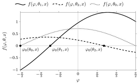
We need to consider the case $0⩽x<1$. Here we need to consider three possible situations: (1) $sin(\pi \theta /2)-x<0$, if $\theta <{\theta }_0$, (2) $sin(\pi \theta /2)-x=0$, if $\theta ={\theta }_0$, (3) $sin(\pi \theta /2)-x>0$, if $\theta >{\theta }_0$. Here ${\theta }_0=(2/\pi )arcsinx$. We will introduce the notation as follows $f(\phi ,\theta ,x)=xsin\phi +cos(\phi +\pi \theta /2)$. In view of this notation, the condition in Equation (33) will take the form $f(\phi ,\theta ,x)>0$. In Figure 1 the function graph $f(\phi ,\theta ,x)$ is plotted for $0⩽x<1$ with different values of the parameter $\theta$ that correspond to three possible situations: $\theta <{\theta }_0$, $\theta ={\theta }_0$, $\theta >{\theta }_0$.

Figure 1. The graph of the function $f(\phi ,\theta ,x)$ at $x<1$ (the curve is plotted at $x=0.7$) and different values of the parameter $\theta$: ${\theta }_0=(2/\pi )arcsinx$, ${\theta }_1<{\theta }_0$, ${\theta }_2>{\theta }_0$. Heavy dots demonstrate the value of the solution of the Equation $f(\phi ,\theta ,x)=0$ for values $\theta ={\theta }_0,{\theta }_1,{\theta }_2$.

Let us consider the case $\theta <{\theta }_0$. In Figure 1, a curve $f(\phi ,{\theta }_1,x)$ corresponds to this case. From this figure one can see that the condition $f(\phi ,\theta ,x)>0$ is met for values $\phi >{\phi }_0(\theta ,x)$. We need to remind that ${\phi }_0(\theta ,x)$ is the solution of the Equation (38). Thus, choosing the principal branch of the function $arctanx$ we get $\pi /2⩾\phi >max(-\pi /2,{\phi }_0(\theta ,x))$ or

$${\phi }_0(\theta ,x)<\phi ⩽\pi /2,0⩽x<1,\theta <{\theta }_0.$$

(39)

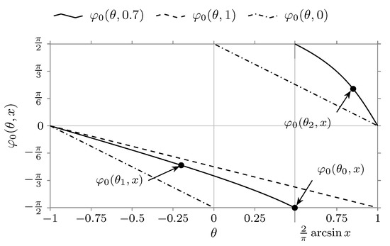
This condition is easy to determine from Figure 2. The values of $\phi$ lying above the curve ${\phi }_0(\theta ,x)$ and not exceeding the value $\pi /2$ correspond to the condition $f(\phi ,\theta ,x)>0$ at $\theta <{\theta }_0$.

Figure 2. The graph of the function ${\phi }_0(\theta ,x)$ at $x⩽1$. The figure shows the graphs for values $x=0,0.7,1$. Heavy dots designate the values of this function with the value of the parameter $\theta ={\theta }_0,{\theta }_1,{\theta }_2$ and $x=0.7$ corresponding to Figure 1.

In the case of $x=0$, we get ${\theta }_0=0$ and ${\phi }_0(\theta ,0)=arctan(cot(\pi \theta /2))$. Therefore, the condition $\theta <{\theta }_0$ will take the form $\theta <0$. One should pay attention that the argument $\pi \theta /2$ at $-1⩽\theta ⩽1$ takes the values in the range from $-\pi /2$ to $\pi /2$. In this range of values $cot(\pi \theta /2)$ in the point $\theta =0$ has the point of discontinuity. We will write ${\phi }_0(\theta ,0)$ in the form

$${\phi }_0(\theta ,0)=arctan(1/tan(\pi \theta /2)).$$

(40)

and will make use of the following trigonometric identities

$$arctany=\left\{\begin{array}{cc}\mathrm{arccot}(1/y)-\pi ,\hfill & y⩽0,\hfill \\ \mathrm{arccot}(1/y),\hfill & y>0\hfill \end{array}\right.$$

(41)

and

$$arctany+\mathrm{arccot}y=\pi /2.$$

(42)

Now using these two trigonometric identities in Equation (40), we find

$${\phi }_0(\theta ,x)=-\frac{\pi }{2}-\frac{\pi \theta }{2},\theta <0$$

(43)

Thus, at $x=0$ the condition in Equation (39) will take the form $-\frac{\pi }{2}-\frac{\pi \theta }{2}<\phi ⩽\frac{\pi }{2}$, if $\alpha =1$ and $\theta <0$. The condition obtained is the same as the condition in Equation (29), if to limit the latter above with the value $\pi /2$ at $\theta <0$.

Now we need to consider the case $\theta ={\theta }_0$. In Figure 2 we can see that when increasing the parameter $\theta$ the point ${\phi }_0(\theta ,x)$ will approach the value $-\pi /2$. With such a change of the parameter $\theta$ the function graph $f(\phi ,\theta ,x)$ in Figure 1 will shift to the left and with the value $\theta ={\theta }_0$ will take the form that is given in Figure 1. As we can see from Figure 2, in this case the function ${\phi }_0(\theta ,x)$ has a discontinuity in the point $\theta ={\theta }_0$. It is connected with the fact that the principal branch of the function $arctanx$ is investigated. In the vicinity of this point we have ${lim}_{\theta \to {\theta }_0-0}{\phi }_0(\theta ,x)={lim}_{\theta \to {\theta }_0-0}arctan\left(\frac{cos(\pi \theta /2)}{sin(\pi \theta /2)-x}\right)=-\frac{\pi }{2}$ and ${lim}_{\theta \to {\theta }_0+0}{\phi }_0(\theta ,x)={lim}_{\theta \to {\theta }_0+0}arctan\left(\frac{cos(\pi \theta /2)}{sin(\pi \theta /2)-x}\right)=\frac{\pi }{2}$. From this we can see that the point ${\theta }_0$ is the point of discontinuity of the first kind. It is possible to eliminate the discontinuity of the function ${\phi }_0(\theta ,x)$ in the point ${\theta }_0$ by defining the value of this function in the given point. We will select

$${\phi }_0({\theta }_0,x)=-\pi /2,0⩽x<1.$$

(44)

Thus, the condition in Equation (33) is met if

$$-\pi /2<\phi <\pi /2,0⩽x<1,\theta ={\theta }_0.$$

(45)

It should be noted that there are precisely strict inequalities here. In fact, if to take $\phi =\pm \pi /2$, then in the case considered these values will be the solution of the Equation (38) which will lead to divergence of the integral in Equation (31).

Now we will consider the case $\theta >{\theta }_0$. From Figure 1 one can see that by increasing the parameter $\theta$ from ${\theta }_0$ to 1 the half-period of the function $f(\phi ,\theta ,x)$ satisfying the condition $f(\phi ,\theta ,x)>0$ will keep moving to the left. At the same time, the left point which is the solution of an equation $f(\phi ,\theta ,x)=0$ will become smaller than $-\pi /2$. Since we take interest in the interval from $-\pi /2$ to $\pi /2$, then the left bound of the interval will be the value $-\pi /2$. Keeping in mind that the half-period of the function $f(\phi ,\theta ,x)$ is equal to $\pi$, the right bound of the interval $f(\phi ,\theta ,x)>0$ will be the second solution of the equation $f(\phi ,\theta ,x)=0$. As a result, the case considered the condition in Equation (33) will be met with values $\phi$ satisfying the inequality

$$-\pi /2⩽\phi <{\phi }_0(\theta ,x),0⩽x<1,\theta >{\theta }_0.$$

(46)

The graph of the function ${\phi }_0(\theta ,x)$ is given in Figure 2.

If $x=0$, we have ${\theta }_0=0$ and condition $\theta >{\theta }_0$ turns into a condition $\theta >0$. As it was pointed out earlier, in this case it is convenient to represent ${\phi }_0(\theta ,x)$ in the form of Equation (40). Now using the trigonometric identities in Equations (41) and (42) in Equation (40) we obtain

$${\phi }_0(\theta ,x)=\frac{\pi }{2}-\frac{\pi \theta }{2},\theta >0.$$

(47)

Thus, at $x=0$ the condition in Equation (46) takes the form $-\frac{\pi }{2}⩽\phi <\frac{\pi }{2}-\frac{\pi \theta }{2}$, if $x=0$ and $\theta >0$. The condition obtained is the same as the condition in Equation (29), if to limit the latter below with a value $-\pi /2$ at $\theta >0$.

If now we put together the expressions in Equations (43), (44), and (47), then ${\phi }_0(\theta ,0)$ takes the form

$${\phi }_0(\theta ,0)=\left\{\begin{array}{cc}-\pi /2-\pi \theta /2,\hfill & \theta ⩽0\hfill \\ \pi /2-\pi \theta /2,\hfill & \theta >0.\hfill \end{array}\right.$$

The graph of the function ${\phi }_0(\theta ,0)$ is given in Figure 2.

Consider now the case $x=1$. In this case the inequality in Equation (35) has the form

$$tan\phi (1-sin(\pi \theta /2\left)\right)>-cos(\pi \theta /2).$$

(48)

From this it follows that $1-sin(\pi \theta /2)>0$, for any $\theta <{\theta }_0$, where ${\theta }_0=(2/\pi )arcsin1=1$. As a result, selecting the principal branch of the function $arctany$, the inequality in Equation (48) takes the form

$${\phi }_0(\theta ,x)<\phi ⩽\pi /2,x=1,-1⩽\theta <1.$$

(49)

This inequality gives a condition under which the inequality will be satisfied in Equation (35) in case $x=1$. The graph of the function ${\phi }_0(\theta ,1)$ is given in Figure 2.

Thus, the inequalities in Equations (36), (39), (45), (46), and (49) completely define the condition under which the inequality is satisfied in Equation (33). Combining these conditions for Equation (32), we obtain

$$\underset{R\to \infty }{lim}U(R,\phi ,1,\theta )=0,\mathrm{if}\left\{\begin{array}{cc}{\phi }_0(\theta ,x)<\phi ⩽\pi /2,& x>1,-1⩽\theta ⩽1,\hfill \\ {\phi }_0(\theta ,x)<\phi ⩽\pi /2,& 0⩽x<1,\theta <{\theta }_0,\hfill \\ -\pi /2<\phi <\pi /2,& 0⩽x<1,\theta ={\theta }_0,\hfill \\ -\pi /2⩽\phi <{\phi }_0(\theta ,x),& 0⩽x<1,\theta >{\theta }_0,\hfill \\ {\phi }_0(\theta ,x)<\phi ⩽\pi /2,& x=1,-1⩽\theta <1,\hfill \end{array}\right.$$

(50)

where ${\theta }_0=(2/\pi )arcsinx$. It should be noted that if $\phi ={\phi }_0(\theta ,x)$, then in this case $xsin\phi +cos(\phi +\pi \theta /2)=0$ and, as a consequence, ${lim}_{R\to \infty }U(R,{\phi }_0(\theta ,x),1,\theta )=\infty$. Therefore, $\phi \ne {\phi }_0(\theta ,x)$. In addition, in terms of Equation (34), one should exclude the case $x=1,\theta =1$ from consideration.

Now using Equation (50) in Equation (31), we ultimately obtain

$$I\left(C_R\right)\underset{R\to \infty }{\to }0\mathrm{if}\left\{\begin{array}{cc}{C}_R=\{z:\left|z\right|=R,{\phi }_0(\theta ,x)+\epsilon ⩽argz⩽\pi /2\},\hfill & x>1,-1⩽\theta ⩽1,\hfill \\ C_R=\{z:\left|z\right|=R,{\phi }_0(\theta ,x)+\epsilon ⩽argz⩽\pi /2\},\hfill & 0⩽x<1,-1⩽\theta <{\theta }_0,\hfill \\ C_R=\left\{z:\left|z\right|=R,-\pi /2+\epsilon ⩽argz⩽\pi /2-\epsilon \right\},\hfill & 0⩽x<1,\theta ={\theta }_0,\hfill \\ C_R=\{z:\left|z\right|=R,-\pi /2⩽argz⩽{\phi }_0(\theta ,x)-\epsilon \},\hfill & 0⩽x<1,{\theta }_0<\theta ⩽1,\hfill \\ C_R=\{z:\left|z\right|=R,{\phi }_0(\theta ,x)+\epsilon ⩽argz⩽\pi /2\},\hfill & x=1,-1⩽\theta <1,\hfill \end{array}\right.$$

where $\epsilon$ is any arbitrary small positive number. This proves items 5, 6, 7, 8, and 9 of the lemma and proves the lemma completely. □

Remark 1.

The statements of the Lemma 2 are preserved if to substitute contours $C_R$ with their parts.

Using the lemma which was proved one can substantiate the validity of transition from an integral ${\int }_0^{\infty }exp\left\{itx\right\}\widehat{g}(t,\alpha ,\theta )dt$ along the real variable t to an integral ${\int }_{\Gamma }exp\left\{izx\right\}{g}^{+}(z,\alpha ,\theta )dz$ in the complex variable z along some contour $\Gamma$ for inversion formulas in Equation (9). We will state this result in the form of a lemma.

Lemma 3.

Let us consider the family of contours $\{\Gamma \}$ in the complex plane z with a cut along a half-line $argz=-\pi$ satisfying the following conditions:

1. 

Every contour starts in the point $z=0$.

2. 

None of the contours Γ intersects the lines of the cut.

3. 

Moving from the point $z=0$ along the contour Γ we let it tend to infinity but in such a way that starting from some place all points $z\in \Gamma$ have values of arguments within the limits:

$$\begin{array}{cc}\hfill 0⩽argz⩽\pi -\epsilon ,& if0<\alpha <1,-1⩽\theta ⩽1,x>0,\hfill \end{array}$$

(51)

$$\begin{array}{cc}\hfill -\frac{\pi }{2\alpha }-\frac{\pi \theta }{2}+\epsilon ⩽argz⩽\frac{\pi }{2\alpha }-\frac{\pi \theta }{2},& if1<\alpha ⩽2,\left|\theta \right|⩽(2/\alpha -1),x>0,\hfill \end{array}$$

(52)

$$\begin{array}{cc}\hfill -\frac{\pi }{2\alpha }-\frac{\pi \theta }{2}+\epsilon ⩽argz⩽\frac{\pi }{2\alpha }-\frac{\pi \theta }{2}-\epsilon ,& if0<\alpha ⩽2,x=0,\left|\theta \right|⩽min(1,2/\alpha -1),\hfill \end{array}$$

(53)

$$\begin{array}{cc}\hfill {\phi }_0(\theta ,x)+\epsilon ⩽argz⩽\frac{\pi }{2},& if\alpha =1,x>1,-1⩽\theta ⩽1,\hfill \end{array}$$

(54)

$$\begin{array}{cc}\hfill -\frac{\pi }{2}⩽argz⩽{\phi }_0(\theta ,x)-\epsilon ,& if\alpha =1,0⩽x<1,{\theta }_0<\theta ⩽1,\hfill \end{array}$$

(55)

$$\begin{array}{cc}\hfill -\frac{\pi }{2}+\epsilon ⩽argz⩽\frac{\pi }{2}-\epsilon ,& if\alpha =1,0⩽x<1,\theta ={\theta }_0,\hfill \end{array}$$

(56)

$$\begin{array}{cc}\hfill {\phi }_0(\theta ,x)+\epsilon ⩽argz⩽\frac{\pi }{2},& if\alpha =1,0⩽x<1,-1⩽\theta <{\theta }_0,\hfill \end{array}$$

(57)

$$\begin{array}{cc}\hfill {\phi }_0(\theta ,x)+\epsilon ⩽argz⩽\frac{\pi }{2},& if\alpha =1,x=1,-1⩽\theta <1,\hfill \end{array}$$

(58)

where ${\theta }_0=(2/\pi )arcsinx$ and ${\phi }_0(\theta ,x)$ have the form in Equation (12) and $\epsilon >0$ is any arbitrary small number. Then for any contour of the specified type and any pair of admissible parameters $(\alpha ,\theta )$ and any $x⩾0$ (with the exception of the point $x=1,\alpha =1,\theta =1$)

$${\int }_0^{\infty }{e}^{itx}g(t,\alpha ,-\theta )dt={\int }_{\Gamma }{e}^{izx}{g}^{+}(z,\alpha ,-\theta )dz,$$

(59)

where t is real.

Proof. 

From constraints imposed on contours $\Gamma$ one can see that it is possible to divide the whole family of contours $\{\Gamma \}$ into two kinds. The contours which start in the point $z=0$ and tend to infinity without intersecting the positive part of a real semiaxis are referred to the contours of the first kind. The contours intersecting the positive part of a real semiaxis are referred to the contours of the second kind.

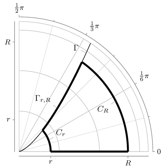
We will consider, at first, contours of the first kind. We will introduce the following notation: $z_r$ is the intersection point of the contour $\Gamma$ with a circle $\left|z\right|=r$, $C_r$ is an arc of a circle of radius r (not crossing the cut) which is formed when moving from the point $z=r$ to the point $z_r$ and ${\Gamma }_{r,R}$ is a part of a contour $\Gamma$ which is formed when moving from the point $z_r$ to the point $z_R$. We form a closed contour $G_{r,R}=[r,R]\cup C_R\cup {\overline{\Gamma }}_{r,R}\cup C_r$ (see Figure 3). The line means that we go along the contour in the opposite direction. Since the function $h\left(z\right)=e^{izx}{g}^{+}(z,\alpha ,-\theta )$ is analytic in the region restricted by the contour $G_{r,R}$, then by using the Cauchy theorem

$${\int }_{G_{r,R}}h\left(z\right)dz={\int }_r^{R}h\left(z\right)dz+{\int }_{C_R}h\left(z\right)dz-{\int }_{{\Gamma }_{r,R}}h\left(z\right)dz+{\int }_{C_r}h\left(z\right)dz=0.$$

Figure 3. Auxiliary contour $G_{r,R}$ (heavy curve).

We will assume in this expression that $r\to 0$ and $R\to \infty$. Using Lemma 2 and Remark 1 we find that ${\int }_{C_R}h\left(z\right)dz+{\int }_{C_r}h\left(z\right)dz\to 0$, at $R\to \infty$ and $r\to 0$. Therefore, the equality in Equation (59) is true.

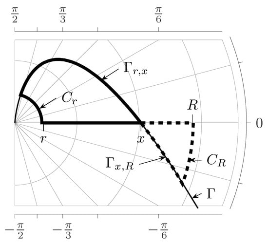
Now consider the contours of the second kind. These contours are characterized by the feature that they intersect the real axis. Therefore, to prove the lemma, we consider two closed auxiliary contours: the contour $G_{r,x}=[r,x]\cup {\overline{\Gamma }}_{r,x}\cup C_r$ and contour $G_{x,R}=\overline{[x,R]}\cup C_R\cup {\Gamma }_{x,R}$ (see Figure 4). Here x is the intersection point of a contour $\Gamma$ with a real axis. Since the function $h\left(z\right)$ is analytic within the regions restricted with the contours ${\Gamma }_{r,x}$ and ${\Gamma }_{x,R}$, then by using the Cauchy theorem

$$\begin{array}{cc}\hfill {\int }_{G_{x,r}}h\left(z\right)dz=& {\int }_r^{x}h\left(z\right)dz-{\int }_{{\Gamma }_{r,x}}h\left(z\right)dz+{\int }_{C_r}h\left(z\right)dz=0,\hfill \end{array}$$

(60)

$$\begin{array}{cc}\hfill {\int }_{G_{x,R}}h\left(z\right)dz=& -{\int }_x^{R}h\left(z\right)dz+{\int }_{{\Gamma }_{x,R}}h\left(z\right)dz+{\int }_{C_R}h\left(z\right)dz=0.\hfill \end{array}$$

(61)

Figure 4. Auxiliary contours $G_{r,x}$ (heavy curve) and $G_{x,R}$ (dashed heavy curve).

Now we will assume in these expressions that $r\to 0$ and $R\to \infty$. Using Lemma 2 and Remark 1, we find that ${\int }_{C_r}h\left(z\right)dz\to 0$ at $r\to 0$ and ${\int }_{C_R}h\left(z\right)dz\to 0$ at $R\to \infty$. Now summing up Equations (60) and () in view of this result we obtain

$${\int }_0^{x}h\left(z\right)dz+{\int }_x^{\infty }h\left(z\right)dz={\int }_{{\Gamma }_{0,x}}h\left(z\right)dz+{\int }_{{\Gamma }_{x,\infty }}h\left(z\right)dz,$$

hence, the equality in Equation (59) is true. □

The following lemma will be useful further

Lemma 4.

For any $x⩾0$ and any $-1⩽\theta ⩽1$ the function

$$\phi (\theta ,x)=arctan\left(\frac{x-sin\left(\frac{\pi }{2}\theta \right)}{cos\left(\frac{\pi }{2}\theta \right)}\right)$$

(62)

and function ${\phi }_0(\theta ,x)$, defined by (12), are connected with relations between each other:

1. 

if $x⩾1$, then

$${\phi }_0(\theta ,x)=\phi (\theta ,x)-\pi /2;$$

(63)

2. 

if $0⩽x<1$, then

$${\phi }_0(\theta ,x)=\left\{\begin{array}{cc}\phi (\theta ,x)-\pi /2,\hfill & -1⩽\theta ⩽{\theta }_0,\hfill \\ \phi (\theta ,x)+\pi /2,\hfill & {\theta }_0<\theta ⩽1,\hfill \end{array}\right.$$

(64)

where ${\theta }_0=(2/\pi )arcsinx$.

Proof. 

Let us consider the case $x>1$. Using the identity in Equation (42) as well as the identity

$$\mathrm{arccot}(-y)=\pi -\mathrm{arccot}\left(y\right),$$

(65)

we obtain

$${\phi }_0(\theta ,x)=arctan\left(\frac{cos(\pi \theta /2)}{sin(\pi \theta /2)-x}\right)=\frac{\pi }{2}-\mathrm{arccot}\left(\frac{cos(\pi \theta /2)}{sin(\pi \theta /2)-x}\right)=-\frac{\pi }{2}+\mathrm{arccot}\left(\frac{cos(\pi \theta /2)}{x-sin(\pi \theta /2)}\right).$$

Since $x>1$, then the argument $\frac{cos(\pi \theta /2)}{x-sin(\pi \theta /2)}>0$ for any $-1⩽\theta ⩽1$. Now using the identity in Equation (41) for $y>0$ we get

$${\phi }_0(\theta ,x)=\phi (\theta ,x)-\pi /2,x>1,-1⩽\theta ⩽1.$$

(66)

Consider the case $x=1$. In the same way as in our previous case, using the identities in Equations (42) and (65), we find

$${\phi }_0(\theta ,1)=arctan\left(\frac{cos(\pi \theta /2)}{sin(\pi \theta /2)-1}\right)=-\frac{\pi }{2}+\mathrm{arccot}\left(\frac{cos(\pi \theta /2)}{1-sin(\pi \theta /2)}\right).$$

(67)

From this expression one can see that the argument $\frac{cos(\pi \theta /2)}{1-sin(\pi \theta /2)}⩾0$ for any $-1⩽\theta <1$ and it has an indeterminate form $0/0$ at $\theta =1$. Evaluating indeterminate forms according to L’Hôpital’s rule we get ${lim}_{\theta \to 1-0}\frac{cos(\pi \theta /2)}{1-sin(\pi \theta /2)}=\infty$. Consequently, $cos(\pi \theta /2)/(1-sin(\pi \theta /2\left)\right)⩾0$, if $-1⩽\theta ⩽1$. Now using in Equation (67) the identity of Equation (41) for $y>0$, we obtain

$${\phi }_0(\theta ,1)=\phi (\theta ,1)-\pi /2,-1⩽\theta ⩽1.$$

Combining now this expression and the expression of Equation (66) we come to Equation (63). Thus, the first item of the lemma is proved.

Now we will consider the case $0⩽x<1$. Using the identities in Equations (42) and (65) we get

$${\phi }_0(\theta ,x)=arctan\left(\frac{cos(\pi \theta /2)}{sin(\pi \theta /2)-x}\right)=-\frac{\pi }{2}+\mathrm{arccot}\left(\frac{cos(\pi \theta /2)}{x-sin(\pi \theta /2)}\right).$$

(68)

Taking into consideration that $cos(\pi \theta /2)⩾0$ for any $\theta \in [-1,1]$, we find that the sign of $\frac{cos(\pi \theta /2)}{x-sin(\pi \theta /2)}$ is defined by the denominator. We have three possible situations: (1) $x-sin(\pi \theta /2)<0$, if $\theta >{\theta }_0$, (2) $x-sin(\pi \theta /2)=0$, if $\theta ={\theta }_0$, (3) $x-sin(\pi \theta /2)>0$, if $\theta <{\theta }_0$. Here ${\theta }_0=(2/\pi )arcsinx$. Taking into consideration Equation (44), we obtain $\frac{cos(\pi \theta /2)}{x-sin(\pi \theta /2)}=+\infty$, if $\theta ={\theta }_0$. Thus, $\frac{cos(\pi \theta /2)}{x-sin(\pi \theta /2)}⩽0$, if $\theta >{\theta }_0$, and $\frac{cos(\pi \theta /2)}{x-sin(\pi \theta /2)}⩾0$, if $\theta ⩽{\theta }_0$. Now in Equation (68) applying the identity in Equation (41) we get

$${\phi }_0(\theta ,x)=\left\{\begin{array}{cc}-\frac{\pi }{2}+arctan\left(\frac{x-sin(\pi \theta /2)}{cos(\pi \theta /2)}\right),\hfill & \theta ⩽{\theta }_0,\hfill \\ -\frac{\pi }{2}+\pi +arctan\left(\frac{x-sin(\pi \theta /2)}{cos(\pi \theta /2)}\right),\hfill & \theta >{\theta }_0.\hfill \end{array}\right.$$

From here it follows Equation (64). The lemma is completely proved. □

In Figure 5 and Figure 6, the graphs of the functions ${\phi }_0(\theta ,x)$ and $\phi (\theta ,x)$ are given for the cases $x⩾1$ and $0⩽x<1$ which clearly illustrate the validity of the lemma that has just been proved.

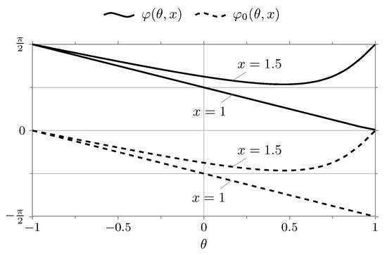
Figure 5. The graph of the function $\phi (\theta ,x)$ and ${\phi }_0(\theta ,x)$ depending on the parameter $\theta$ in the case of $x⩾1$ (The graphs are plotted for $x=1.5$ and $x=1$).

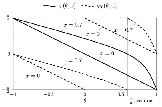
Figure 6. The graph of the function $\phi (\theta ,x)$ and ${\phi }_0(\theta ,x)$ depending on the parameter $\theta$ in the case $x<1$ (The graphs are plotted for $x=0.7$ and $x=0$).

3. Main Results

Now we can formulate the main theorem which gives an integral representation for the probability density of a stable law $g(x,\alpha ,\theta )$ with the characteristic function in Equation (1).

Theorem 1.

The distribution density $g(x,\alpha ,\theta )$ of a strictly stable law with a characteristic function as in Equation (1) can be represented in the form

1. 

If $\alpha \ne 1$ and $x\ne 0$ for any values $\left|\theta \right|⩽min(1,2/\alpha -1)$

$$g(x,\alpha ,\theta )=\frac{\alpha }{\pi |\alpha -1|}{\int }_{-\pi {\theta }^{*}/2}^{\pi /2}exp\left\{-{\left|x\right|}^{\alpha /(\alpha -1)}U(\phi ,\alpha ,{\theta }^{*})\right\}U(\phi ,\alpha ,{\theta }^{*}){\left|x\right|}^{1/(\alpha -1)}d\phi ,$$

(69)

where ${\theta }^{*}=\theta \mathrm{sign}x$ and

$$U(\phi ,\alpha ,\theta )={\left(\frac{sin\left(\alpha \left(\phi +\frac{\pi }{2}\theta \right)\right)}{cos\phi }\right)}^{\alpha /(1-\alpha )}\frac{cos\left(\phi (1-\alpha )-\frac{\pi }{2}\alpha \theta \right)}{cos\phi }.$$

(70)

2. 

If $x=0$, then for any $0<\alpha ⩽2$ and $\left|\theta \right|⩽min(1,2/\alpha -1)$

$$g(0,\alpha ,\theta )=\frac{1}{\pi }cos\left(\pi \theta /2\right)\Gamma \left(1/\alpha +1\right)$$

(71)

3. 

If $\alpha =1$, then for any $\left|\theta \right|⩽1$ and any values x

$$g(x,1,\theta )=\frac{cos(\pi \theta /2)}{\pi (x^2-2xsin(\pi \theta /2)+1)}.$$

(72)

Proof. 

To obtain the expression for the probability density we use the inversion formulas in Equation (9). In principle, it makes no difference which formula to use. The result will differ then only by the sign of the parameter $\theta$. We will use the first formula in Equation (9), we have

$$g(x,\alpha ,\theta )=\frac{1}{\pi }\Re {\int }_0^{\infty }{e}^{itx}\widehat{g}(t,\alpha ,-\theta )dt.$$

(73)

Without loss of generality, we assume that $x>0$. The density $g(x,\alpha ,\theta )$ for $x<0$ can be obtained with the inversion property in Equation (7). Next, let us make the substitution of integration variable $t\to z$, where z is complex-valued. Such a substitution means that we analytically extend the integral to the complex plane. With this analytical continuation is carried out starting with the positive part of a real semiaxis. As a result, we have that $\widehat{g}(t,\alpha ,-\theta )\to g^{+}(z,\alpha ,-\theta )$, where $g^{+}(z,\alpha ,\theta )$ is defined by Equation (11). The improper integral becomes the integral along the contour $\Gamma$. We will define the contour $\Gamma$ in such a way that $\Im e^{izx}{g}^{+}(z,\alpha ,\theta )=0$, and the contour itself $\Gamma$ should start in the point $z=0$ tend to infinity. Since in the inversion formula of Equation (73) the variable is $t>0$ then from this it follows that $argz$ must lie within the limits $-\pi /2⩽argz⩽\pi /2$. As result, the contour $\Gamma$ will take the form

$$\Gamma =\{z:\Im e^{izx}{g}^{+}(z,\alpha ,\theta )=0,-\frac{\pi }{2}⩽argz⩽\frac{\pi }{2},|z|⩾0\},$$

(74)

However, the specific type of the contour has to be defined. In view of the foregoing, the expression in Equation (73) will be written in the form

$$g(x,\alpha ,\theta )=\frac{1}{\pi }\Re {\int }_{\Gamma }exp\{izx-z^{\alpha }exp\left\{i\frac{\pi }{2}\alpha \theta \right\}\}dz.$$

(75)

As a result, the problem consists in determining the contour form $\Gamma$, in proving the validity of transition from Equation (73) to Equation (75) and in calculating this integral.

Let us consider the case $\alpha \ne 1$. Representing $z=r{e}^{i\phi }$ and using this representation in Equation (75) for the intergrand we obtain

$$\begin{array}{c}exp\{izx-z^{\alpha }exp\left\{i\frac{\pi }{2}\alpha \theta \right\}\}=exp\left\{ixr{e}^{i\phi }-r^{\alpha }{e}^{i\alpha \phi }exp\left\{i\frac{\pi }{2}\alpha \theta \right\}\right\}=\hfill \\ \hfill exp\{-rxsin\phi -r^{\alpha }cos\left(\alpha (\phi +\frac{\pi }{2}\theta )\right)\}exp\left\{i[rxcos\phi -r^{\alpha }sin\left(\alpha (\phi +\frac{\pi }{2}\theta )\right)]\right\}.\end{array}$$

(76)

From the condition $\Im e^{izx}{g}^{+}(z,\alpha ,\theta )=0$ and $-\frac{\pi }{2}⩽argz⩽\frac{\pi }{2}$ follows that

$$rxcos\phi -r^{\alpha }sin\left(\alpha (\phi +\frac{\pi }{2}\theta )\right)=0.$$

(77)

The solution of this equation is in an explicit form

$$r\left(\phi \right)={\left(\frac{sin\left(\alpha (\phi +\frac{\pi }{2}\theta )\right)}{xcos\left(\phi \right)}\right)}^{\frac{1}{1-\alpha }}.$$

(78)

This expression determines the form of contour integration $\Gamma$.

We will determine the admissible region $argz\equiv \phi$. From the condition $\left|z\right|⩾0$ follows that $(sin\left(\alpha (\phi +\frac{\pi }{2}\theta )\right))/(xcos\left(\phi \right))⩾0$. Taking into account that $x>0$ we obtain that the condition $r\left(\phi \right)>0$ is met if $sin\left(\alpha (\phi +\frac{\pi }{2}\theta )\right)⩾0$ and $cos\phi ⩾0$. From the condition $sin\left(\alpha (\phi +\frac{\pi }{2}\theta )\right)⩾0$ we obtain that $-\frac{\pi }{2}\theta ⩽\phi ⩽\frac{\pi }{\alpha }-\frac{\pi }{2}\theta$, and from the condition $cos\phi ⩾0$ we get that $-\frac{\pi }{2}⩽\phi ⩽\frac{\pi }{2}$. Combining these two inequalities we obtain

$$max\left(-\frac{\pi }{2},-\frac{\pi }{2}\theta \right)⩽\phi ⩽min\left(\frac{\pi }{2},\frac{\pi }{\alpha }-\frac{\pi }{2}\theta \right).$$

(79)

Taking into consideration that at $0<\alpha <1$ the parameter $\theta$ takes values from the range $-1⩽\theta ⩽1$ and at $1<\alpha ⩽2$ from the range $-(\frac{2}{\alpha }-1)⩽\theta ⩽\frac{2}{\alpha }-1$ we obtain that $max\left(-\frac{\pi }{2},-\frac{\pi }{2}\theta \right)=-\frac{\pi }{2}\theta$ and $min\left(\frac{\pi }{2},\frac{\pi }{\alpha }-\frac{\pi }{2}\theta \right)=\frac{\pi }{2}$. Using this result in Equation (79) we get $-\pi \theta /2⩽\phi ⩽\pi /2$. Taking account of this condition and the expression in Equation (78) we obtain that in the case $\alpha \ne 1$ the contour $\Gamma$ takes the form

$$\Gamma =\left\{z:r\left(\phi \right)={\left(\frac{sin\left(\alpha (\phi +\frac{\pi }{2}\theta )\right)}{xcos\left(\phi \right)}\right)}^{\frac{1}{1-\alpha }},-\frac{\pi }{2}\theta ⩽\phi ⩽\frac{\pi }{2},\alpha \ne 1\right\}.$$

(80)

We consider now the contour form $\Gamma$ with different values of parameters. Replacing the boundary values $\phi$ in the expression for $r\left(\phi \right)$, we obtain

$$\begin{array}{cc}r\left(-\frac{\pi }{2}\theta \right)=0,r\left(\frac{\pi }{2}\right)=\infty ,\hfill & \mathrm{at}0<\alpha <1\hfill \\ r\left(-\frac{\pi }{2}\theta \right)=\infty ,r\left(\frac{\pi }{2}\right)=0,\hfill & \mathrm{at}1<\alpha ⩽2.\hfill \end{array}$$

(81)

Thus, at $0<\alpha <1$ the contour $\Gamma$ starts in the point $z=0$ at $\phi =-\frac{\pi }{2}\theta$ and tends to infinity at $\phi =\frac{\pi }{2}$. In the case $1<\alpha ⩽2$ the situation is opposite: the contour $\Gamma$ starts in the point $z=0$ at $\phi =\frac{\pi }{2}$ and tends to infinity at $\phi =-\frac{\pi }{2}\theta$.

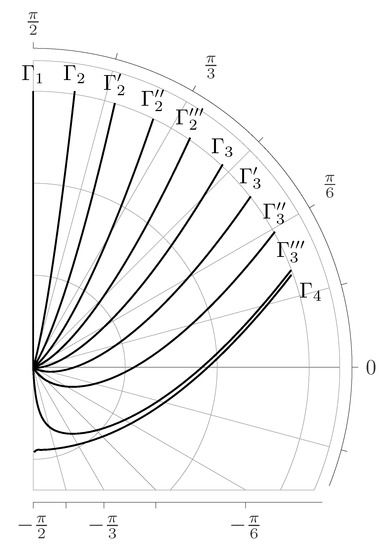
As we can see the contours $\Gamma$ described in Equation (80) with different values of the parameter $\theta$ differ in its type (see Figure 7 and Figure 8). They can be divided into 7 main groups.

Figure 7. The type of a contour $\Gamma$ at $\alpha \in (0,1)$ and various values of parameter $\theta$. The contours are given for the case $\alpha =0.6$ and ${\Gamma }_1$ - $\theta =-1$, ${\Gamma }_2$ - $\theta =-0.75$, ${\Gamma }_2^{\prime }$ - $\theta =-0.5$, ${\Gamma }_2^{″}$ - $\theta =-0.25$, ${\Gamma }_2^{‴}$ - $\theta =0$, ${\Gamma }_3$ - $\theta =0.25$, ${\Gamma }_3^{\prime }$ - $\theta =0.5$, ${\Gamma }_3^{″}$ - $\theta =0.75$, ${\Gamma }_3^{‴}$ - $\theta =0.98$, ${\Gamma }_4$ - $\theta =1$.

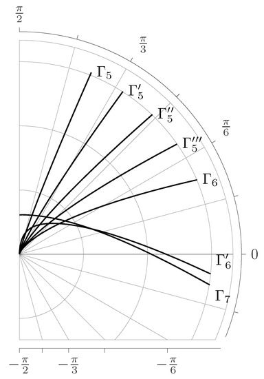
Figure 8. The type of a contour $\Gamma$ at $\alpha \in (1,2]$ and with different values of the parameter $\theta$. The contours are given for the case $\alpha =1.25$ and ${\Gamma }_5$ - $\theta =-0.6$, ${\Gamma }_5^{\prime }$ - $\theta =-0.4$, ${\Gamma }_5^{″}$ - $\theta =-0.2$, ${\Gamma }_5^{‴}$ - $\theta =0$, ${\Gamma }_6$ - $\theta =0.2$, ${\Gamma }_6^{\prime }$ - $\theta =0.57$, ${\Gamma }_7$ - $\theta =0.6$.

The contours of the first group are made up of the contours with values $0<\alpha <1$ and $\theta =-1$. In Figure 7 the contour ${\Gamma }_1$ corresponds to this case. From the definition of the contour in Equation (80) one can see that in this case the admissible region of an angle $\phi$ takes the form $\frac{\pi }{2}⩽\phi ⩽\frac{\pi }{2}$. This means that the contour goes along the positive part of the imaginary axis: $\Gamma \equiv {\Gamma }_1=I^{+}$.

The contours of the second group include the contours with values $0<\alpha <1$ and $-1<\theta ⩽0$. In Figure 7 the contours ${\Gamma }_2,{\Gamma }_2^{\prime },{\Gamma }_2^{″},{\Gamma }_2^{‴}$ are referred to this case. The contours of this group start in the point $z=0$ at $\phi =-\frac{\pi }{2}\theta$ and tend to infinity at $\phi \to \frac{\pi }{2}$. As one can see, in this case $-\frac{\pi }{2}\theta ⩾0$, and contours of this group do not cross the real semiaxis.

The third group is made up of the contours with values of parameters $0<\alpha <1$ and $0<\theta <1$. In Figure 7 this group consists of the contours ${\Gamma }_3,{\Gamma }_3^{\prime },{\Gamma }_3^{″},{\Gamma }_3^{‴}$. The contours of this group start in the point $z=0$ coming out at an angle $\phi =-\frac{\pi }{2}\theta$, and tend to infinity at $\phi \to \frac{\pi }{2}$. As we can see in this case $-\frac{\pi }{2}\theta <0$. Therefore, the contours of this group approach the point $z=0$ at values of $\phi <0$ which, in its turn, means that these contours intersect the positive part of the real axis.

The fourth group is composed of the contours $0<\alpha <1$, $\theta =1$. In Figure 7 the contour ${\Gamma }_4$. corresponds to this case. From the expression in Equation (78) we can see that in this case at $\phi \to -\frac{\pi }{2}$ in this expression there is an indeterminate form $0/0$. Evaluating this indeterminate form according to L’Hôpital’s rule we get ${lim}_{\phi \to -\frac{\pi }{2}}r\left(\phi \right)={(\alpha /x)}^{1/(1-\alpha )}$. Thus, the contours of this group start in the point $z=-i{(\alpha /x)}^{1/(1-\alpha )}$ at $\phi =-\frac{\pi }{2}$ and tend to infinity at $\phi \to \pi /2$. As we can see the contours of this group also cross the positive part of the real axis.

5. 

The fifth group includes the contours with parameters $1<\alpha ⩽2$ and $-(2/\alpha -1)⩽\theta ⩽0$. In Figure 8 the contours ${\Gamma }_5,{\Gamma }_5^{\prime },{\Gamma }_5^{″},{\Gamma }_5^{‴}$ are referred to this case. The contours of this group start in the point $z=0$ at $\phi =\pi /2$ and tend to infinity at $\phi \to -\frac{\pi }{2}\theta$. Since in this case $\theta ⩽0$, then the condition $\phi >0$ is met for all points of the contour. Therefore, the contours of this group do not cross the positive part of the real axis.

5. 

The sixth group consists of the contours with parameters $1<\alpha ⩽2$, $0<\theta <2/\alpha -1$. In Figure 8 the contours ${\Gamma }_6,{\Gamma }_6^{\prime }$ correspond to this case. The contours of this groups start in the point $z=0$ at $\phi =\pi /2$ and tend to infinity at $\phi \to -\frac{\pi }{2}\theta$. Since in this case $\theta >0$, then $-\frac{\pi }{2}\theta <0$ and, consequently, the contours of this group cross the positive part of the real semiaxis.

5. 

The seventh group comprises the contours with parameters $1<\alpha ⩽2$ and $\theta =2/\alpha -1$. In Figure 8 the contour ${\Gamma }_7$ corresponds to this case. One should pay attention that in this case at $\phi =\pi /2$ the function $r\left(\phi \right)$ defined by Equation (78) has an indeterminate form $0/0$. Evaluating this indeterminate form according to L’Hôpital’s rule we obtain ${lim}_{\phi \to \pi /2}r\left(\phi \right)={(\alpha /x)}^{1/(1-\alpha )}$. Thus, the contours of this group start in the point $z=i{(\alpha /x)}^{1/(1-\alpha )}$ at $\phi =\pi /2$ and tend to infinity at $\phi \to -\frac{\pi }{2}\theta$. The contours of this group also cross the positive part of the real axis.

This indicates that the contours of the first, second and third groups ($0<\alpha <1,-1⩽\theta <1$) and contours of the fifth and sixth groups ($1<\alpha ⩽2,-(2/\alpha -1)⩽\theta <2/\alpha -1$) satisfy the conditions of the Lemma 3. In fact, the contours of these groups start in the point $z=0$, do not cross the line of the cut that goes through a half-line $argz=-\pi$ and tend to infinity. The contours of the first, second, third groups tend to infinity at $\phi =\frac{\pi }{2}$. This means that the contours of these groups satisfy the condition in Equation (51). The contours of the fifth and sixth groups tend to infinity at $\phi =-\frac{\pi }{2}\theta$. Thus, these contours satisfy the condition in Equation (52).

Consider the contours of the fourth group ${\Gamma }_4$. The contours of this group start in the point $z=-i{(\alpha /x)}^{1/(1-\alpha )}$ and tend to infinity at $\phi \to \frac{\pi }{2}$. Consider an auxiliary contour ${\Gamma }^{*}=\{z:argz=-\pi /2,0⩽|z|⩽{(\alpha /x)}^{1/(1-\alpha )}\}$. With the help of a contour ${\Gamma }^{*}$ we form a new contour $S={\Gamma }^{*}\bigcup {\Gamma }_4$. The specific feature of the contour ${\Gamma }^{*}$ is then that $\Im exp\{izx-z^{\alpha }exp\left\{i\frac{\pi }{2}\alpha \theta \right\}\}=0$ for $z\in {\Gamma }^{*}$. From this it follows that

$$\frac{1}{\pi }\Re {\int }_{{\Gamma }^{*}}exp\{izx-z^{\alpha }exp\left\{i\frac{\pi }{2}\alpha \theta \right\}\}dz=0.$$

Therefore, for the case $0<\alpha <1,\theta =1$ we get

$$\frac{1}{\pi }\Re {\int }_{S}exp\{izx-z^{\alpha }exp\left\{i\frac{\pi }{2}\alpha \theta \right\}\}dz=\frac{1}{\pi }\Re {\int }_{{\Gamma }_4}exp\{izx-z^{\alpha }exp\left\{i\frac{\pi }{2}\alpha \theta \right\}\}dz.$$

(82)

However, now the contour $S={\Gamma }^{*}\bigcup {\Gamma }_4$ completely satisfies the conditions of the Lemma 3: it starts in the point $z=0$ without crossing the line of the cut and tends to infinity at $\phi =\pi /2$.

For the contours of the seventh froup ${\Gamma }_7$ we do the same. Consider an auxiliary contour ${\Gamma }^{**}=\{z:argz=\pi /2,0⩽|z|⩽{(x/\alpha )}^{1/(\alpha -1)}\}$. With the help of this contour we form the contour $S^{*}={\Gamma }^{**}\bigcup {\Gamma }_7$. Now, the contour $S^{*}$ completely satisfies the conditions of the Lemma 3. As in the previous case $\Im exp\{izx-z^{\alpha }exp\left\{i\frac{\pi }{2}\alpha \theta \right\}\}=0$ for $z\in {\Gamma }^{**}$. From this it follows

$$\frac{1}{\pi }\Re {\int }_{{\Gamma }^{**}}exp\{izx-z^{\alpha }exp\left\{i\frac{\pi }{2}\alpha \theta \right\}\}dz=0.$$

As a result, for the case $1<\alpha ⩽2,\theta =2/\alpha -1$ we get

$$\frac{1}{\pi }\Re {\int }_{S^{*}}exp\{izx-z^{\alpha }exp\left\{i\frac{\pi }{2}\alpha \theta \right\}\}dz=\frac{1}{\pi }\Re {\int }_{{\Gamma }_7}exp\{izx-z^{\alpha }exp\left\{i\frac{\pi }{2}\alpha \theta \right\}\}dz.$$

(83)

Now, applying Lemma 3 and taking account of the equalities in Equations (82) and (83) we find that

$$\frac{1}{\pi }\Re {\int }_0^{\infty }{e}^{itx}\widehat{g}(t,\alpha ,-\theta )dt=\frac{1}{\pi }{\int }_{\Gamma }{e}^{izx}{g}^{+}(z,\alpha ,-\theta )dz,$$

(84)

where the contour $\Gamma$ is defined by the expression in Equation (80). As a result, an improper integral along the positive part of the real axis in the expression of Equation (73) can be replaced with an integral along the contour $\Gamma$. Thus, in the case considered ($\alpha \ne 1$) we showed the validity of transition from Equation (73) to Equation (75).

Returning to Equation (75), taking into consideration Equation (76) and representing complex z in the form $z=r{e}^{i\phi }$, we obtain

$$\begin{array}{c}g(z,\alpha ,\theta )=\frac{1}{\pi }\Re {\int }_{\Gamma }exp\{izx-z^{\alpha }exp\left\{i\frac{\pi }{2}\alpha \theta \right\}\}dz=\frac{1}{\pi }{\int }_{\Gamma }\Re exp\{izx-z^{\alpha }exp\left\{i\frac{\pi }{2}\alpha \theta \right\}\}d(\Re z)=\hfill \\ \hfill \frac{1}{\pi }{\int }_{\Gamma }exp\{-rxsin\phi -r^{\alpha }cos\left(\alpha (\phi +\frac{\pi }{2}\theta )\right)\}cos\left(rxcos\phi -r^{\alpha }sin\left(\alpha (\phi +\frac{\pi }{2}\theta )\right)\right)d[rcos\phi ].\end{array}$$

We will place here the expression in Equation (78). One should pay attention that in this case the Equation (77) is valid, consequently, we obtain

$$g(x,\alpha ,\theta )=\frac{1}{\pi }{\int }_{\Gamma }exp\left\{A\left(\phi \right)\right\}d[r\left(\phi \right)cos\phi ],$$

(85)

where $A\left(\phi \right)=-r\left(\phi \right)xsin\phi -r{\left(\phi \right)}^{\alpha }cos\left(\alpha (\phi +\frac{\pi }{2}\theta )\right)$ and $r\left(\phi \right)$ is defined by Equation (78). We transform the function $A\left(\phi \right)$

$$\begin{array}{c}A\left(\phi \right)=-x{\left(\frac{sin\left(\alpha (\phi +\frac{\pi }{2}\theta )\right)}{xcos\left(\phi \right)}\right)}^{1/(1-\alpha )}sin\phi -{\left(\frac{sin\left(\alpha (\phi +\frac{\pi }{2}\theta )\right)}{xcos\left(\phi \right)}\right)}^{\alpha /(1-\alpha )}cos\left(\alpha (\phi +\frac{\pi }{2}\theta )\right)\hfill \\ \hfill =-x^{\alpha /(\alpha -1)}{\left(\frac{sin\left(\alpha (\phi +\frac{\pi }{2}\theta )\right)}{cos\left(\phi \right)}\right)}^{\alpha /(1-\alpha )}\frac{cos\left(\phi (1-\alpha )-\frac{\pi }{2}\alpha \theta \right)}{cos\phi }=-x^{\alpha /(\alpha -1)}U(\phi ,\alpha ,\theta ),\end{array}$$

(86)

where $U(\phi ,\alpha ,\theta )$ has the form of Equation (70).

Now we consider the differential, we have $d\left[r\right(\phi )cos\phi ]=cos\phi d\left[r\right(\phi \left)\right]-r\left(\phi \right)sin\phi d\phi$. For the differential $d\left[r\right(\phi \left)\right]$ we get

$$d\left[r\left(\phi \right)\right]=d\left[{\left(\frac{sin\left(\alpha (\phi +\frac{\pi }{2}\theta )\right)}{xcos\left(\phi \right)}\right)}^{1/(1-\alpha )}\right]=\frac{r\left(\phi \right)}{1-\alpha }\left(\alpha cot\left(\alpha \left(\phi +\frac{\pi }{2}\theta \right)\right)+tan\phi \right)d\phi .$$

Using now this result in the expression for $d\left[r\right(\phi )cos\phi ]$, we have

$$\begin{array}{c}d[r\left(\phi \right)cos\phi ]=\frac{r\left(\phi \right)}{1-\alpha }cos\phi \left(\alpha cot\left(\alpha \left(\phi +\frac{\pi }{2}\theta \right)\right)+tan\phi \right)d\phi -r\left(\phi \right)sin\phi d\phi \hfill \\ =\frac{\alpha r\left(\phi \right)}{1-\alpha }\left(cos\phi cot\left(\alpha \left(\phi +\frac{\pi }{2}\theta \right)\right)+sin\phi \right)d\phi \\ \hfill =\frac{\alpha }{1-\alpha }{\left(\frac{sin\left(\alpha \left(\phi +\frac{\pi }{2}\theta \right)\right)}{xcos\phi }\right)}^{1/(1-\alpha )}\frac{cos\left(\alpha \left(\phi +\frac{\pi }{2}\theta \right)-\phi \right)}{sin\left(\alpha \left(\phi +\frac{\pi }{2}\theta \right)\right)}d\phi =\frac{\alpha }{1-\alpha }{x}^{1/(\alpha -1)}U(\phi ,\alpha ,\theta )d\phi ,\end{array}$$

(87)

where $U(\phi ,\alpha ,\theta )$ has the form of Equation (70).

Now using Equations (86) and (87) in Equation (85) and also taking into consideration that the motion along the contour $\Gamma$, having the form of Equation (80) now described by the parameter change $\phi$, we obtain

$$g(x,\alpha ,\theta )=\frac{\alpha }{\pi (1-\alpha )}{\int }_{{\phi }_{min}}^{{\phi }_{max}}exp\left\{-x^{\alpha /(\alpha -1)}U(\phi ,\alpha ,\theta )\right\}{x}^{1/(\alpha -1)}U({\phi }_{\alpha },\theta )d\phi$$

(88)

From the expression in Equation (84) one can see that the integration limits ${\phi }_{min}$ and ${\phi }_{max}$ should be selected in such a way that the motion along the contour $\Gamma$ could correspond to a change from $r=0$ to $r=\infty$. From the expression in Equation (81) it is clear that in the case $0<\alpha <1$ a change in the angle $\phi$ from $-\frac{\pi }{2}\theta$ to $\frac{\pi }{2}$ corresponds to the motion along the contour $\Gamma$ from $r=0$ to $r=\infty$. Therefore, in this case ${\phi }_{min}=-\frac{\pi }{2}\theta$, ${\phi }_{max}=\frac{\pi }{2}$. In the case $1<\alpha ⩽2$ a change in the angle $\phi$ from $\frac{\pi }{2}$ to $-\frac{\pi }{2}\theta$ corresponds to the motion from $r=0$ to $r=\infty$. Therefore, in this case ${\phi }_{min}=\frac{\pi }{2}$, and ${\phi }_{max}=-\frac{\pi }{2}\theta$. Combining these two cases the expression in Equation (88) takes the form

$$g(x,\alpha ,\theta )=\frac{\alpha }{\pi |1-\alpha |}{\int }_{-\frac{\pi }{2}\theta }^{\frac{\pi }{2}}exp\left\{-x^{\alpha /(\alpha -1)}U(\phi ,\alpha ,\theta )\right\}{x}^{1/(\alpha -1)}U(\phi ,\alpha ,\theta )d\phi ,\alpha \ne 1.$$

(89)

It should be pointed out that this formula was obtained on the assumption $x>0$. The case $x<0$ is easy to obtain using the property of inversion for the density of probabilities in Equation (7). For this it is enough to replace the parameter $\theta$ in the formula in Equation (89) with $-\theta$. It is possible to combine these two cases if in the formula of Equation (89) to substitute the parameter $\theta$ for the parameter ${\theta }^{*}=\theta \mathrm{sign}x$ and the value x is taken in absolute value. As a result, we obtain the expression in Equation (69) valid for any $x\ne 0$ and any admissible $\alpha \ne 1$.

Now we consider the case $0<\alpha ⩽2$ and $x=0$. In this case the inversion formula of Equation (75) takes the form

$$g(0,\alpha ,\theta )=\frac{1}{\pi }\Re {\int }_{\Gamma }exp\left\{-z^{\alpha }exp\left\{\frac{\pi }{2}\alpha \theta \right\}\right\}dz,$$

(90)

where the contour $\Gamma$ is determined by the expression in Equation (74), but it is necessary to determine the specific type of a contour in the case under consideration.

We represent the complex number z in the form $z=r{e}^{i\phi }$. As a result, the integrand in Equation (90) takes the form

$$exp\left\{-z^{\alpha }exp\left\{\frac{\pi }{2}\alpha \theta \right\}\right\}=exp\left\{-r^{\alpha }cos\left(\alpha \left(\phi +\frac{\pi }{2}\theta \right)\right)-i{r}^{\alpha }sin\left(\alpha \left(\phi +\frac{\pi }{2}\theta \right)\right)\right\}.$$

(91)

Using the condition $\Im g^{+}(0,\alpha ,\theta )=0$, we obtain

$$r^{\alpha }sin\left(\alpha \left(\phi +\frac{\pi }{2}\theta \right)\right)=0.$$

(92)

This equation has two solutions: $r=0$, for any $\phi$, and $\phi =-\pi \theta /2$, $r⩾0$. It is clear that if $r=0$, then $\Im g^{+}(0,\alpha ,\theta )=0$ for any value of $\phi$, for definiteness we will select $\phi =-\pi \theta /2$ if $r=0$. As a result, the contour of integration of Equation (74) takes the form $\Gamma =\{z:|z|⩾0,argz=-\pi \theta /2\}$, where $\left|\theta \right|⩽min(1,2/\alpha -1)$, $0<\alpha ⩽2$. From this it is clear that in the case under consideration the family of contours $\Gamma$ are represented by half-lines starting from the point $z=0$ at an angle $argz=-\pi \theta /2$. Consequently, the family of contours $\Gamma$ satisfy items 1 and 2 of Lemma 3 and also the condition in Equation (53) in item 3. Thus, we substantiate the transition from the improper integral of Equation (73) to the contour integral in Equation (90).

Now we put the expression in Equation (91) in Equation (90) and taking into account Equation (92), we obtain

$$g(0,\alpha ,\theta )=\frac{1}{\pi }{\int }_{\Gamma }exp\left\{-r^{\alpha }cos\left(\alpha \left(\phi +\frac{\pi }{2}\theta \right)\right)\right\}\Re \left[dz\right]=\frac{cos(\pi \theta /2)}{\pi }{\int }_0^{\infty }exp\left\{-r^{\alpha }\right\}dr.$$

Here it was taken into account that $\Re \left[dz\right]=cos(\pi \theta /2)dr$ on the contour $\Gamma$. The limits of integration were selected in such a way that when moving along the contour r could change from 0 to ∞. Since the contour $\Gamma$ in the case under consideration is a half-line coming out of the point $z=0$ at an angle $argz=-\pi \theta /2$, then the motion along the contour $\Gamma$ from 0 to ∞ corresponds to a change r from 0 to ∞. Making in this integral a substitution of a variable $r^{\alpha }=y$ and using the definition of the gamma-function $\Gamma \left(n\right)={\int }_0^{\infty }{t}^{n-1}{e}^{-t}dt$, $n>0$ we obtain the expression Equation (71). Thus, the second item of the theorem is proved.

Now we consider the case $\alpha =1$. We will make an assumption that $x⩾0$. In this case, the inversion formula in Equation (75) takes the form

$$g(x,1,\theta )=\frac{1}{\pi }\Re {\int }_{\Gamma }exp\left\{izx-zexp\left\{i\frac{\pi }{2}\theta \right\}\right\}dz,$$

(93)

where the contour of integration defined by Equation (74) will be written in the form

$$\Gamma =\{z:\Im e^{izx}{g}^{+}(z,1,\theta )=0,\frac{\pi }{2}⩽argz⩽\frac{\pi }{2},|z|⩾0\},$$

(94)

Here it should be noted that analytic continuation of the function $\widehat{g}(t,1,-\theta )$ from the positive part of the real axis t to the complex plane z at $\alpha =1$ is an analytic function and it has the form $g^{+}(z,1,-\theta )=exp\left\{-zexp\left\{i\frac{\pi }{2}\theta \right\}\right\}$.

As in the previous case, we begin by defining the form of the integration contour $\Gamma$. Consider the integrand in Equation (93) and we represent the complex number z in the form $z=r{e}^{i\phi }$. As a result, we obtain

$$\begin{array}{c}exp\{izx-zexp\left\{i\frac{\pi }{2}\theta \right\}\}=exp\left\{ixr{e}^{i\phi }-r{e}^{i\phi }exp\left\{i\frac{\pi }{2}\theta \right\}\right\}=\hfill \\ \hfill exp\{-r\left(xsin\phi +cos\left((\phi +\frac{\pi }{2}\theta )\right)\right)\}exp\left\{ir\left(xcos\phi -sin\left((\phi +\frac{\pi }{2}\theta )\right)\right)\right\}.\end{array}$$

(95)

From this expression we get that the condition $\Im e^{izx}{g}^{+}(z,1,-\theta )=0$ leads to an equation

$$r\left(xcos\phi -sin\left((\phi +\frac{\pi }{2}\theta )\right)\right)=0.$$

(96)

This equation has two solutions. The first solution is $r=0$. The second solution we obtain from the equation $xcos\phi -sin\left((\phi +\frac{\pi }{2}\theta )\right)=0$, $r⩾0$. Solving it with respect to $\phi$ we get

$$\phi (\theta ,x)=arctan\left(\frac{x-sin(\pi \theta /2)}{cos(\pi \theta /2)}\right).$$

(97)

As a result, the contour of integration in Equation (94) takes the form

$$\Gamma =\left\{z:argz=\phi (\theta ,x),\left|z\right|⩾0,-1⩽\theta ⩽1\right\}$$

(98)

Thus, the contours $\Gamma$ with different values $\theta$ are half-lines coming out of the origin at an angle $\phi (\theta ,x)$ and tending to infinity.

Next, it is necessary to substantiate the transition from the integral in Equation (73) to the integral along the contour in Equation (93). For this we will use Lemmas 3 and 4. From the definition in Equation (98), it is clear that for all admissible values $\theta$ and $x⩾0$ the contour $\Gamma$ satisfies item 1 and 2 of the Lemma 3. There is only one thing left, to find out if the contour in Equation (98) satisfies item 3 of this lemma.

Consider the case $x>1$ at first. According to item 3 of the Lemma 3 for the equality in Equation (59) to be valid the contour of Equation (98) must satisfy the condition in Equation (54). Now using the Lemma 4. According to this lemma in the case $x⩾1$ the functions $\phi (\theta ,x)$ and ${\phi }_0(\theta ,x)$ are connected between each other with a ratio (63) from which it directly follows that ${\phi }_0(\theta ,x)<\phi (\theta ,x)$ for all $\theta \in [-1,1]$. Therefore, at $x>1$ the condition in Equation (54) is met and we can move from the integral in Equation (73) to the integral in Equation (93). In the case $x=1$ the contour $\Gamma$ must meet the condition in Equation (58). Now using the Lemma 4 we obtain that in this case for all $\theta \in [-1,1]$ the inequality ${\phi }_0(\theta ,x)<\phi (\theta ,x)$ is true. Therefore, in this case the condition in Equation (58) is satisfied. Now we consider the case $0⩽x<1$. Similar to previous case, applying the Lemma 4 namely, the formula in Equation (64) we get that in this case the contour in Equation (98) satisfies the conditions in Equations (55)–(57) Lemma 3. Thus, the contour in Equation (98) completely satisfies the conditions of the Lemma 3 and therefore, the equality

$$\frac{1}{\pi }\Re {\int }_0^{\infty }{e}^{itx}\widehat{g}(t,1,-\theta )dt=\frac{1}{\pi }{\int }_{\Gamma }{e}^{izx}{g}^{+}(z,1,-\theta )dz$$

is true. This makes it possible to replace the improper integral in the expression of Equation (73) over the real variable with the integral over the contour $\Gamma$. Thus, the possibility for the transition from the formula in Equation (73) to the formula in Equation (75) is substantiated. We need to note that in the case under consideration $\alpha =1$ the expression in Equation (75) takes the form of Equation (93). It should also be pointed out that that due to Equation (34) the case $\alpha =1,\theta =1,x=1$ is excluded in the Lemma 3. That is why, here, this case should also be excluded from consideration.

Now taking into account Equation (95), the expression of Equation (93) will be written in the following form

$$\begin{array}{c}g(x,1,\theta )=\frac{1}{\pi }\Re {\int }_{\Gamma }exp\{-r\left(xsin\phi +cos(\phi +\frac{\pi }{2}\theta )\right)\}exp\left\{ir\left(xcos\phi -sin(\phi +\frac{\pi }{2}\theta )\right)\right\}dz=\hfill \\ \hfill \frac{1}{\pi }{\int }_{\Gamma }exp\{-r\left(xsin\phi +cos(\phi +\frac{\pi }{2}\theta )\right)\}cos\left\{r\left(xcos\phi -sin(\phi +\frac{\pi }{2}\theta )\right)\right\}\Re \left[dz\right]\end{array}$$

Now using here the definition of Equation (98) we obtain that $\Re \left[dz\right]=cos\left(\phi \right(\theta ,x\left)\right)dr$. The motion along the contour $\Gamma$ should take place in such a way that it would start in the point $z=0$ in the process of moving it would tend to infinity. Therefore, the motion from $r=0$ to $r=\infty$ corresponds to such motion. Taking into consideration that on the contour $\Gamma$ the condition of Equation (96) is met, we obtain

$$g(x,1,\theta )=\frac{1}{\pi }{\int }_0^{\infty }exp\{-r\left(xsin\phi (\theta ,x)+cos(\phi (\theta ,x)+\frac{\pi }{2}\theta )\right)\}cos\left(\phi (\theta ,x)\right)dr$$

As we can see, the integral obtained is easy to calculate. As a result, we obtain

$$g(x,1,\theta )=\frac{1}{\pi }\frac{cos\left(\phi \right(\theta ,x\left)\right)}{xsin\phi (\theta ,x)+cos\left(\phi \right(\theta ,x)+\pi \theta /2)}.$$

Using now the definition of the function $\phi (\theta ,x)$ (97) after simple transformations we get

$$g(x,1,\theta )=\frac{cos(\pi \theta /2)}{\pi \left(x^2-2xsin(\pi \theta /2)+1\right)}.$$

(99)

Recall that consideration was carried out for the case $x⩾0$. The case $x<0$ can be obtained using the inversion property for the density of probability of Equation (7). For this it is enough to replace $\theta$ with $-\theta$. It is possible to combine these two cases if to introduce a parameter ${\theta }^{*}=\theta \mathrm{sign}x$. However, we want to note that if to perform this replacement in the expression of Equation (99), then the expression itself will not change $g(x,1,\theta )\to g(x,1,{\theta }^{*})\equiv g(x,1,\theta ).$ Consequently, the formula in Equation (99) is true for any x. Thus, the theorem is completely proved. □

We will make some remarks on the proved theorem.

Remark 2.

The proof of the case $\alpha =1$ was carried out under the assumption $x⩾0$. Therefore, the formula in Equation (99) was obtained for the case $x⩾0$. The generalization of this formula for the case $x<0$ was carried out using the inversion property $g(-x,1,\theta )=g(x,1,-\theta )$. It should be noted here that in the process of proving this case the point $\theta =1$, $x=1$ was excluded from consideration. Therefore, in view of the inversion property, the point $\theta =-1$, $x=-1$ should also be excluded. In these two points the density $g(x,1,\theta )$ has a peculiarity. In fact, substituting the value $\theta =\pm 1$, we obtain

$$g(x,1,\pm 1)=\frac{cos(\pi /2)}{\pi {(x\mp 1)}^2}=\left\{\begin{array}{cc}0,\hfill & x\ne \pm 1,\hfill \\ 0/0,\hfill & x=\pm 1.\hfill \end{array}\right.$$

However, an indeterminate form $0/0$ can be evaluated in the following remark.

Remark 3.

Equations (71) and (72) can be obtained directly from the inversion formulas in Equation (9) without resorting to analytic continuation of the characteristic function $\widehat{g}(t,\alpha ,\theta )$ to the complex plane with the subsequent transition from the improper integral over the real variable (73) to the integral along the contour in Equation (75). We first consider the case $\alpha =1$. Using the inversion formula (the first formula in Equation (9)) we obtain

$$g(x,1,\theta )=\frac{1}{\pi }\Re {\int }_0^{\infty }{e}^{itx}\widehat{g}(t,1,-\theta )dt=\frac{1}{\pi }\Re {\int }_0^{\infty }exp\left\{t\left(ix-exp\left\{i\frac{\pi }{2}\theta \right\}\right)\right\}dt=\frac{1}{\pi }\Re I,$$

(100)

where $I={\int }_0^{\infty }exp\left\{t\left(ix-exp\left\{i\frac{\pi }{2}\theta \right\}\right)\right\}dt$. We determine under which conditions this integral will converge. For the integral I the inequality is valid

$$\left|I\right|⩽{\int }_0^{\infty }\left|exp\left\{t\left(ix-exp\left\{i\frac{\pi }{2}\theta \right\}\right)\right\}\right|dt$$

(101)

For the integrand we have

$$\left|exp\left\{t\left(ix-exp\left\{i\frac{\pi }{2}\theta \right\}\right)\right\}\right|=exp\left\{-tcos(\pi \theta /2)\right\}cos\left(t(x-sin(\pi \theta /2))\right).$$

(102)

Since in the case considered ($\alpha =1$) the parameter θ varies within the limits $-1⩽\theta ⩽1$, we obtain $cos(\pi \theta /2)>0,if-1<\theta <1$. From here we get ${lim}_{t\to \infty }\left|exp\left\{t\left(ix-exp\left\{i\frac{\pi }{2}\theta \right\}\right)\right\}\right|=0$, if $-1<\theta <1$. Thus, the integral in Equation (101) will converge, and, therefore, and the integral I will also converge at $-1<\theta <1$.

We consider now the cases $\theta =\pm 1$. If $\theta =1$, then from Equation (102) we obtain

$$\left|exp\left\{t\left(ix-exp\{i\pi /2\}\right)\right\}\right|=cos\left(t(x-1)\right).$$

(103)

Substituting this result in Equation (101) we get

$$\left|I\right|⩽{\int }_0^{\infty }cos\left(t(x-1)\right)dt=\left\{\begin{array}{cc}0,\hfill & x\ne 1\hfill \\ \infty ,\hfill & x=1.\hfill \end{array}\right.$$

(104)

Similarly, if $\theta =-1$, we have

$$\left|I\right|⩽{\int }_0^{\infty }cos\left(t(x+1)\right)dt=\left\{\begin{array}{cc}0,\hfill & x\ne -1\hfill \\ \infty ,\hfill & x=-1.\hfill \end{array}\right.$$

(105)

Thus, at $\theta =\pm 1$ the integral $I=0$ for all $x\ne \pm 1$, and integral I will diverge in the points $x=1,\theta =1$ and $x=-1,\theta =-1$.

Returning to Equation (100) and by calculating the integral directly, we get

$$\begin{array}{c}g(x,1,\theta )=\frac{1}{\pi }\Re {\int }_0^{\infty }exp\left\{t\left(ix-exp\left\{i\frac{\pi }{2}\theta \right\}\right)\right\}dt=-\frac{1}{\pi }\Re \frac{1}{ix-exp\{i\pi \theta /2\}}\hfill \\ \hfill =-\frac{1}{\pi }\Re \frac{-ix-exp\{-i\pi \theta /2\}}{(ix-exp\{i\pi \theta /2\left\}\right)(-ix-exp\{-i\pi \theta /2\left\}\right)}=\frac{1}{\pi }\frac{cos(\pi \theta /2)}{x^2-2xsin(\pi \theta /2)+1}.\end{array}$$

(106)

From the formula obtained it is clear that if $\theta =\pm 1$

$$g(x,1,\pm 1)=\frac{cos(\pi /2)}{\pi {(x\mp 1)}^2}=\left\{\begin{array}{cc}0,\hfill & x\ne \pm 1\hfill \\ \infty ,\hfill & x=\pm 1.\hfill \end{array}\right.$$

(107)

Thus the behavior of the formula in Equation (106) coincides with the behavior of the integral I in Equations (104) and (105) in the cases $\theta =\pm 1$. Therefore, the formula in Equation (106) is true for any $-1⩽\theta ⩽1$. The expression in Equation (107) means that the density $g(x,1,\pm 1)$ is a degenerate distribution in the point $x=\pm 1$. In other words,

$$g(x,1,\pm 1)=\delta (x\mp 1).$$

(108)

Thus, the obtained expression in Equation (106) completely coincides with the one previously obtained in the Theorem 1 the density in Equation (72), and the conclusion presented in this remark is an alternative way of deducing this density.

Remark 4.

By a similar method, one can obtain the density value at $x=0$. Using the first formula in Equation (9) and making a substitution of the integration variable $t^{\alpha }=\tau$ we get

$$\begin{array}{c}g(0,\alpha ,\theta )=\frac{1}{\pi }\Re {\int }_0^{\infty }\widehat{g}(t,\alpha ,-\theta )dt=\frac{1}{\pi }\Re {\int }_0^{\infty }exp\left\{-t^{\alpha }exp\left\{i\frac{\pi }{2}\alpha \theta \right\}\right\}dt\hfill \\ =\frac{1}{\alpha \pi }\Re {\int }_0^{\infty }exp\left\{-\tau cos\left(\frac{\pi }{2}\alpha \theta \right)-i\tau sin\left(\frac{\pi }{2}\alpha \theta \right)\right\}{\tau }^{1/\alpha -1}d\tau \\ \hfill =\frac{1}{\alpha \pi }{\int }_0^{\infty }exp\left\{-\tau cos\left(\frac{\pi }{2}\alpha \theta \right)\right\}cos\left(ysin\left(\frac{\pi }{2}\alpha \theta \right)\right){\tau }^{1/\alpha -1}d\tau .\end{array}$$

(109)

To calculate the integral obtained it is necessary to use the formula (see [45], Section 1.5. the Equation (35))

$${\int }_0^{\infty }{t}^{\alpha -1}{e}^{-ctcos\beta }cos(ctsin\beta )dt=\Gamma \left(\alpha \right)c^{-\alpha }cos\left(\alpha \beta \right),c>0,\Re \alpha >0,-\pi /2<\beta <\pi /2.$$

It is clear that the integral in Equation (109) completely satisfies the conditions of this integral. Consequently, using it in Equation (109) we get $g(0,\alpha ,\theta )=\frac{1}{\pi }\Gamma (1/\alpha +1)cos(\pi \theta /2)$. The formula obtained coincides completely with the formula in Equation (71).

We will make another useful remark.

Remark 5.

The Theorem 1 formulates an integral representation for the density of a standard strictly stable law. However, it is useful to have a formula that allows one to convert the density of a standard strictly stable law to the density of a strictly stable law with arbitrary λ. The Property 2 and, in particular, the formula in Equation (8) allows one to obtain such a formula.

In fact, in terms of characteristic functions, the formula in Equation (8) will be written as

$$\widehat{g}(t,\alpha ,\theta ,\lambda )=\widehat{g}\left({\lambda }^{1/\alpha }t,\alpha ,\theta \right).$$

(110)

The density is obtained using the inverse Fourier transform of the characteristic function $g(x,\alpha ,\theta ,\lambda )=\frac{1}{2\pi }{\int }_{-\infty }^{\infty }{e}^{itx}\widehat{g}(t,\alpha ,\theta ,\lambda )dt$. Using now the relation in Equation (110) and changing the integration variable ${\lambda }^{1/\alpha }t=\tau$ we obtain the relation for densities.

$$g(x,\alpha ,\theta ,\lambda )={\lambda }^{-1/\alpha }g(x{\lambda }^{-1/\alpha },\alpha ,\theta ).$$

(111)

Thus, the Theorem 1 defines an integral representation for the probability density of a standard strictly stable law with the characteristic function in Equation (1). Using this representation, we can obtain an integral representation for the distribution function of the standard strictly stable law. We formulate this result as a corollary to the Theorem 1.

Corollary 1.

The distribution function of a stable law $G(x,\alpha ,\theta )$ with the characteristic function in Equation (1) can be represented as

1. 

If $\alpha \ne 1$, then for any $\left|\theta \right|⩽min(1,2/\alpha -1)$ and $x\ne 0$

$$G(x,\alpha ,\theta )=\frac{1}{2}(1-\mathrm{sign}\left(x\right))+\mathrm{sign}\left(x\right)G^{(+)}\left(\right|x|,\alpha ,{\theta }^{*}),$$

(112)

where ${\theta }^{*}=\theta \mathrm{sign}\left(x\right)$,

$$\begin{array}{c}{G}^{(+)}(x,\alpha ,\theta )=1-\frac{(1+\theta )}{4}(1+\mathrm{sign}(1-\alpha ))\hfill \\ \hfill +\frac{\mathrm{sign}(1-\alpha )}{\pi }{\int }_{-\pi \theta /2}^{\pi /2}exp\left\{-x^{\alpha /(\alpha -1)}U(\phi ,\alpha ,\theta )\right\}d\phi ,x>0,\end{array}$$

(113)

and $U(\phi ,\alpha ,\theta )$ is defined by Equation (70).

2. 

If $\alpha =1$, then for any $-1⩽\theta ⩽1$ and any x

$$G(x,1,\theta )=\frac{1}{2}+\frac{1}{\pi }arctan\left(\frac{x-sin(\pi \theta /2)}{cos(\pi \theta /2)}\right).$$

(114)

3. 

If $x=0$, then for any admissible α and θ

$$G(0,\alpha ,\theta )=(1-\theta )/2.$$

(115)

Proof. 

We consider the case $\alpha \ne 1$. It is necessary to obtain the distribution function of a stable law with the characteristic function in Equation (1). For the density of distribution a stable law, one should choose the expression in Equation (89) which defines the density $g(x,\alpha ,\theta )$ for $x>0$. In view of this, we write the distribution function in the form

$$G^{(+)}(x,\alpha ,\theta )=1-{\int }_x^{\infty }g(\xi ,\alpha ,\theta )d\xi ,x>0.$$

Now substituting here Equation (89) we find

$$\begin{array}{c}{G}^{(+)}(x,\alpha ,\theta )=1-\frac{\alpha }{\pi |1-\alpha |}{\int }_{-\pi \theta /2}^{\pi /2}U(\phi ,\alpha ,\theta )d\phi {\int }_x^{\infty }{\xi }^{1/(\alpha -1)}exp\left\{-{\xi }^{\alpha /(\alpha -1)}U(\phi ,\alpha ,\theta )\right\}d\xi \hfill \\ =\left\{\begin{array}{cc}{\displaystyle 1+\frac{\mathrm{sign}(\alpha -1)}{\pi }{\int }_{-\pi \theta /2}^{\pi /2}\left(1-exp\left\{-x^{\alpha /(\alpha -1)}U(\phi ,\alpha ,\theta )\right\}\right)d\phi ,}\hfill & \alpha <1,x>0,\hfill \\ {\displaystyle 1-\frac{\mathrm{sign}(\alpha -1)}{\pi }{\int }_{-\pi \theta /2}^{\pi /2}exp\left\{-x^{\alpha /(\alpha -1)}U(\phi ,\alpha ,\theta )\right\}d\phi ,}\hfill & \alpha >1,x>0.\hfill \end{array}\right.\\ \hfill =\left\{\begin{array}{cc}{\displaystyle 1-\frac{(1+\theta )}{2}+\frac{1}{\pi }{\int }_{-\pi \theta /2}^{\pi /2}exp\left\{-x^{\alpha /(\alpha -1)}U(\phi ,\alpha ,\theta )\right\}d\phi ,}\hfill & \alpha <1,x>0,\hfill \\ {\displaystyle 1-\frac{1}{\pi }{\int }_{-\pi \theta /2}^{\pi /2}exp\left\{-x^{\alpha /(\alpha -1)}U(\phi ,\alpha ,\theta )\right\}d\phi ,}\hfill & \alpha >1,x>0.\hfill \end{array}\right.\end{array}$$

If we combine the cases $\alpha <1$ and $\alpha >1$ we obtain

$$G^{(+)}(x,\alpha ,\theta )=1-\frac{(1+\theta )}{4}(1+\mathrm{sign}(1-\alpha ))+\frac{\mathrm{sign}(1-\alpha )}{\pi }{\int }_{-\pi \theta /2}^{\pi /2}exp\left\{-x^{\alpha /(\alpha -1)}U(\phi ,\alpha ,\theta )\right\}d\phi .$$

This formula defines the distribution function of stable law for the case $x>0$ and $\alpha \ne 1$. The case $x<0$ is reduced to the case $x>0$ using the property of an inversion, namely, the formula in Equation (7) for $G(x,\alpha ,\theta )$. As a result, we get $G^{(-)}(-x,\alpha ,\theta )=1-G^{(+)}(x,\alpha ,-\theta )$, $x>0$. This formula gives the distribution function for negative x. Combining the formulas for $G^{(+)}(x,\alpha ,\theta )$ and $G^{(-)}(-x,\alpha ,\theta )$, we obtain the formula in Equation (112) which is true for any $x\ne 0$ and $\alpha \ne 1$.

We now consider the case $\alpha =1$. According to the definition $G(x,1,\theta )={\int }_{-\infty }^{x}g(\xi ,1,\theta )d\xi$. Substituting the density (72) here and replacing the variable $\xi -sin(\pi \theta /2)=\tau$ we obtain

$$\begin{array}{c}G(x,1,\theta )=\frac{cos(\pi \theta /2)}{\pi }{\int }_{-\infty }^x\frac{d\xi }{{\xi }^2-2\xi sin(\pi \theta /2)+1}\hfill \\ \hfill =\frac{cos(\pi \theta /2)}{\pi }{\int }_{-\infty }^{x-sin(\pi \theta /2)}\frac{d\tau }{{\tau }^2+{cos}^2(\pi \theta /2)}=\frac{1}{2}+\frac{1}{\pi }arctan\left(\frac{x-sin(\pi \theta /2)}{cos(\pi \theta /2)}\right).\end{array}$$

Thus, the second item of the corollary has been proved.

To calculate $G(x,\alpha ,\theta )$ at $x=0$ we use the formula in Equation (113). Performing the passage to the limit $x\to 0$ in this expression we get $G(0,\alpha ,\theta )=(1-\theta )/2$. Since the formula in Equation (113) is valid for $\alpha \ne 1$, then the result obtained is valid only for $\alpha \ne 1$. To calculate $G(0,1,\theta )$ it is necessary to use (114). Substituting the value $x=0$ in (114) we obtain $G(0,1,\theta )=(1-\theta )/2$. Thus, the expression (115) is true for any admissible $\alpha$ and $\theta$. □

We make some remarks on the proved corollary.

Remark 6.

In the Remark 3 it is emphasized that in the case $\alpha =1,\theta =\pm 1$ the density $g(x,1,\pm 1)$ is a degenerate distribution in the point $x=\pm 1$ and has the form of Equation (108). Consequently, for the indicated parameter values, the distribution function $G(x,1,\pm 1)$ will have the form of the Heaviside function $G(x,1,\pm 1)=H(x\mp 1)$. This is directly seen from the form of the distribution function at $\alpha =1$. Indeed, substituting the values $\theta =\pm 1$ in Equation (114), we obtain

$$G(x,1,\pm 1)=\frac{1}{2}+\frac{1}{\pi }arctan\left(\frac{x\mp sin(\pi /2)}{cos(\pi /2)}\right)=\left\{\begin{array}{cc}1,\hfill & x>\pm 1,\hfill \\ 0,\hfill & x<\pm 1\hfill \end{array}\right.=H(x\mp 1).$$

Remark 7.

The proved corollary gives an integral representation for the distribution function of a standard strictly stable law. In order to get the distribution function of a strictly stable law for an arbitrary λ it is necessary to use the Remark 5. By definition $G(x,\alpha ,\theta ,\lambda )={\int }_{-\infty }^{x}g(y,\alpha ,\theta ,\lambda )dy$. Using now the relation in Equation (111) and changing the variable $x{\lambda }^{-1/\alpha }=\tau$ we arrive at the relation

$$G(x,\alpha ,\theta ,\lambda )=G\left(x{\lambda }^{-1/\alpha },\alpha ,\theta \right).$$

It should be noted the density in Equation (72) and distribution function in Equation (114) is not new. These formulas were deduced by V.M. Zolotarev (see § 2.3 in [32]). As we can see, this distribution is the stable law for $\alpha =1$ and any $-1⩽\theta ⩽1$ and it is expressed in terms of elementary functions.

4. The Calculation of the Density and Distribution Function of a Stable Law

Integral representations for the probability density and distribution function of a stable law with the characteristic function in Equation (1) were obtained in the Theorem 1 and Corollary 1. These integral representations in Equations (69) and (112) express the probability density and the distribution function in terms of a definite integral. That is why, using the methods of numerical integration, it is possible to calculate the values of these integrals without much difficulty.

In this paper, to calculate definite integrals in Equations (69) and (112) we used the adaptive Gaussian–Kronrod numerical integration algorithm for 31 points. To implement the program for calculating the functions $g(x,\alpha ,\theta )$ and $G(x,\alpha ,\theta )$ we used the implementation of this algorithm in the gsl library (GNU Scientific Library) of version 1.8 [46]. The calculation results for the functions $g(x,\alpha ,\theta )$ and $G(x,\alpha ,\theta )$ by the Equations (69) and (112) are given in Figure 9, Figure 10, Figure 11, Figure 12, Figure 13 and Figure 14.

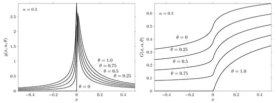
Figure 9. The probability density function $g(x,\alpha ,\theta )$ (on the left) and cumulative distribution function $G(x,\alpha ,\theta )$ (on the right) of a standard strictly stable law with $\alpha =0.3$ and specified values $\theta$.

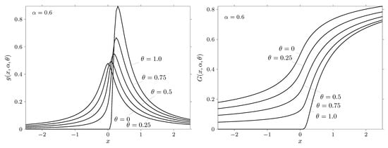
Figure 10. The probability density function $g(x,\alpha ,\theta )$ (on the left) and cumulative distribution function $G(x,\alpha ,\theta )$ (on the right) of a standard strictly stable law with $\alpha =0.6$ and specified values $\theta$.

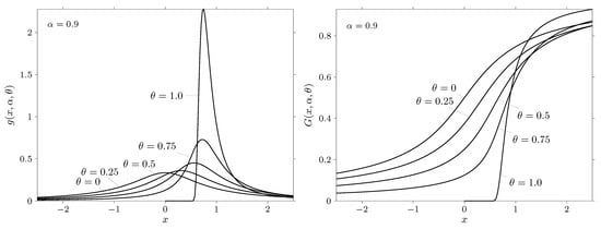
Figure 11. The probability density function $g(x,\alpha ,\theta )$ (on the left) and cumulative distribution function $G(x,\alpha ,\theta )$ (on the right) of a standard strictly stable law with $\alpha =0.9$ and specified values $\theta$.

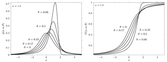
Figure 12. The probability density function $g(x,\alpha ,\theta )$ (on the left) ) and cumulative distribution function $G(x,\alpha ,\theta )$ (on the right) of a standard strictly stable law with $\alpha =1.2$ and specified values $\theta$.

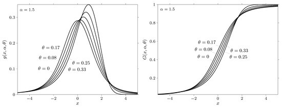
Figure 13. The probability density function $g(x,\alpha ,\theta )$ (on the left) ) and cumulative distribution function $G(x,\alpha ,\theta )$ (on the right) of a standard strictly stable law with $\alpha =1.5$ and specified values $\theta$.

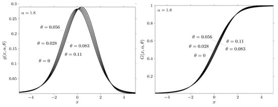
Figure 14. The probability density function $g(x,\alpha ,\theta )$ (on the left) and cumulative distribution function $G(x,\alpha ,\theta )$ (on the right) of a standard strictly stable law with $\alpha =1.8$ and specified values $\theta$.

The figures show the probability density and distribution function for the values of the characteristic exponent $\alpha =0.3,0.6,0.9,1.2,1.5,1.8$ and specified values of the parameter $\theta$ and $\lambda =1$. It should be noted that the admissible region of the parameter $\theta$ is determined by the inequality $\left|\theta \right|⩽min(1,2/\alpha -1)$. Thus, $-1⩽\theta ⩽1$, if $0<\alpha ⩽1$, and $-(2/\alpha -1)⩽\theta ⩽2/\alpha -1$, if $1<\alpha ⩽2$. It is clear that if $\alpha >1$ then the admissible region of the parameter $\theta$ narrows and at $\alpha =2$ the parameter $\theta$ may take a single value $\theta =0$.

Let us analyze the results presented in more detail. We first consider the case $\alpha <1$. The results related to this case are given in Figure 9, Figure 10 and Figure 11. From these figures it can be seen that when $\theta =1$ the probability density is concentrated on the positive semiaxis. Thus, $g(x,\alpha ,1)=0$, $G(x,\alpha ,1)=0$, if $x<0,\alpha <1$. Similarly, for the case $\theta =-1$ and $\alpha <1$, we obtain that the negative semiaxis is the area of concentration of the probability density. Consequently, $g(x,\alpha ,-1)=0,G(x,\alpha ,-1)=1$, if $x>0,\alpha <1$. This result is in complete agreement with remarks 3 and 4 on page 79 of theorem 2.2.3 from the book by [32].

In the introduction, it was noted that in the work [31] (see also [32]) integral representations were obtained for the probability density and distribution function of a stable law with the characteristic function in Equation (5). In order to avoid any confusion the parameters of a stable law with the characteristic function in Equation (5) will be designated as $({\alpha }^{\prime },\beta ,{\lambda }^{\prime },\gamma )$. For the parameters of a strictly stable law with the characteristic function in Equation (1) we keep the notation $(\alpha ,\theta ,\lambda )$. The parameters $({\alpha }^{\prime },\beta ,{\lambda }^{\prime },\gamma )$ are related to the parameters $(\alpha ,\theta ,\lambda )$ by the relations (see [32,36]): ${\alpha }^{\prime }=\alpha$,

$$\begin{array}{ccc}\hfill \theta =\beta K\left({\alpha }^{\prime }\right)/{\alpha }^{\prime },& \lambda ={\lambda }^{\prime },& \mathrm{if}\alpha \ne 1,\hfill \\ \hfill \theta =(2/\pi )arctan(2\gamma /\pi ),& \lambda ={\lambda }^{\prime }{\left({\pi }^2/4+{\gamma }^2\right)}^{1/2},& \mathrm{if}\alpha =1.\hfill \end{array}$$

In the case of $\alpha \ne 1$ from the relation for the parameters $\theta$ and $\beta$ we get $\theta =\beta$, if $\alpha <1$, and $\theta =\beta (1-2/\alpha )$, if $\alpha >1$.

Thus, at $\alpha <1$ the parameters $\theta$ and $\beta$ coincide. Therefore, the corresponding properties for the probability density and the distribution function of stable laws with characteristic functions in Equations (1) and (5) coincide. The situation slightly changes if $\alpha >1$. It can be seen from the above relation that, firstly, the admitted region of the parameter $\theta$ narrows in comparison with the admitted region of the parameter $\beta$, secondly, the parameter $\theta$ changes its sign to the opposite with respect to the parameter $\beta$. Since the parameter $\theta$ has the meaning of an asymmetry parameter, then a change of the sign of this parameter when passing from $\alpha <1$ to $\alpha >1$ will affect the form of probability density. This is clearly seen in Figure 11 and Figure 12 for densities with extreme values of the parameter $\theta$. Comparing densities for the values $\alpha =0.9,\theta =1$ given in Figure 11 and density for the values $\alpha =1.2,\theta =0.66$ given in Figure 12 one can see that these densities are turned into different directions. This fact is a consequence of the fact that the parameter $\theta$ changed the sign compared to the sign of the parameter $\beta$. Thus, for the same sign of the parameter $\theta$ of density $g(x,\alpha ,\theta )$ at $\alpha <1$ and $\alpha >1$ will be turned into different directions. The reason for this behavior is related to the selected parameter system $(\alpha ,\theta ,\lambda )$ of the characteristic function in Equation (1). As it was mentioned in the book by Zolotarev V.M. (see page 19 in [32]), distributions from the class of strictly stable laws are continuous in the totality of their parameters in the entire range of their admissible values it is with this choice of parameters.

It should be pointed out that the Theorem 1 and Corollary 1 formulate expressions for probability density and distribution functions for strict stable laws with a scale parameter $\lambda =1$. To obtain the density and distribution function with an arbitrary value of the scale parameter $\lambda$ it is necessary to use Remarks 5 and 7.

5. Conclusions

In this paper, integral representations for the probability density have been obtained (Theorem 1) and distribution function (Corollary 1) of a standard ($\lambda =1$) strictly stable law with the characteristic function in Equation (1). In the general case $\alpha \ne 1$ and $x\ne 0$ the probability density and distribution function are expressed in terms of a definite integral. In the case $\alpha =1$ for any x and in the case $x=0$ for any admissible $\alpha$ and $\theta$ the probability density and distribution function are expressed in terms of elementary functions. Applying the method of numerical integration, the values of the density and distribution function of strictly stable laws with the characteristic function in Equation (1) were calculated. The calculations show that the numerical methods do not have any difficulties in calculating the density and distribution function for the selected parameter values.

However, this does not mean that one can calculate the density and function of distribution for all admissible parameters by using obtained integral representations. Most likely, numerical integration algorithms will have difficulty in calculating the integral for small values $\alpha$, at $\alpha \approx 1$ and for bigger values of x. The results of the works in which integral representations for densities of stable laws with characteristic functions in Equations (5) and (4) were investigated testify to this. An integral representation for a stable law with the characteristic function in Equation (5) was obtained in the work [31] (see also § 2.2 in [32], § 4.4 in [36]). In the work [33], it was pointed out that when values of $\alpha$ close to 1 problems arise with the numerical calculation of the integral in this integral representation. An integral representation for the density of a stable law with the characteristic function in Equation (4) was obtained in [33]. In this work, it was emphasized that when calculating the density, calculation difficulties arise at values $0<|\alpha -1|<0.02$ and at values $\alpha$ close to zero. In the works by [38,43] the same problems are mentioned when calculating the integral in the representation obtained in the work [33]. Based on this, it should be expected that, with the above parameter values, calculation difficulties will also arise with the density and distribution functions obtained in the Theorem 1 and Corollary 1. In particular, directly from the expressions in Equations (69) and (113), it can be seen that at $\alpha$ close to 1, but not equal to 1, problems may arise with the numerical calculation of the integral. This is indicated by the exponent $\alpha /(\alpha -1)$. It can be seen that when $\alpha \to 1$ this value increases unlimitedly. Most likely, in this case, one will have to look for other ways of calculating the density and distribution function of a strictly stable law.

In conclusion, we would like to point out that the integral representation of the density $g(x,\alpha ,\theta )$ formulated in the Theorem 1 was used to calculate the density in Equation (2). To calculate the improper integral in Equation (2) we used the adaptive quadrature Gaussian–Kornord numerical integration algorithm on 15 points. We used the implementation of this algorithm in the library gsl (GNU Scientific Library) version 1.8 [46]. The calculations performed in some cases show the presence of problems of numerical integration. In particular, at x close to zero, the calculated density behaves like a periodic function. In addition, in some cases, the integration algorithm generates an integration error. All this indicates the need for additional study of the integrand function in Equation (2) and adapting this expression for numerical integration algorithms. It should be noted that the most likely causes of these difficulties may be the ones described above when calculating the density $g(x,\alpha ,\theta )$. Therefore, first of all, it is necessary to find a solution to the problems described above. To calculate the density at x close to zero and for bigger values x the most promising approach is to use an expansion of the strictly stable density in the power series. The method described in the article [43] can be used to calculate the density at $\alpha \to 1$. However, the possibility of using this approach requires additional research.

References

- Kotulski, M. Asymptotic distributions of continuous-time random walks: A probabilistic approach. J. Stat. Phys. 1995, 81, 777–792. [Google Scholar] [CrossRef]
- Kolokoltsov, V.N.; Korolev, V.Y.; Uchaikin, V.V. Fractional Stable Distributions. J. Math. Sci. 2001, 105, 2569–2576. [Google Scholar] [CrossRef]
- Montroll, E.W.; Weiss, G.H. Random Walks on Lattices. II. J. Math. Phys. 1965, 6, 167. [Google Scholar] [CrossRef]
- Scher, H.; Lax, M. Stochastic transport in a disordered solid. I. Theory. Phys. Rev. B 1973, 7, 4491–4502. [Google Scholar] [CrossRef]
- Scher, H.; Lax, M. Stochastic transport in a disordered solid. II. Impurity conduction. Phys. Rev. B 1973, 7, 4502–4519. [Google Scholar] [CrossRef]
- Klafter, J.; Blumen, A.; Shlesinger, M.F. Stochastic pathway to anomalous diffusion. Phys. Rev. A 1987, 35, 3081–3085. [Google Scholar] [CrossRef]
- Metzler, R.; Klafter, J. The random walk’s guide to anomalous diffusion: A fractional dynamics approach. Phys. Rep. 2000, 339, 1–77. [Google Scholar] [CrossRef]
- Zaburdaev, V.Y.; Denisov, S.I.; Klafter, J. Lévy walks. Rev. Mod. Phys. 2015, 87, 483–530. [Google Scholar] [CrossRef]
- Uchaikin, V.V. Montroll-Weiss problem, fractional equations, and stable distributions. Int. J. Theor. Phys. 2000, 39, 2087–2105. [Google Scholar] [CrossRef]
- Saenko, V.V. New Approach to Statistical Description of Fluctuating Particle Fluxes. Plasma Phys. Rep. 2009, 35, 1–13. [Google Scholar] [CrossRef]
- Saenko, V.V. Self-similarity of fluctuation particle fluxes in the plasma edge of the stellarator L-2M. Contrib. Plasma Phys. 2010, 50, 246–251. [Google Scholar] [CrossRef]
- Saenko, V.; Saenko, Y. Approximation of Microarray Gene Expression Profiles by the Stable Laws. Int. J. Environ. Eng. 2015, 2, 98–102. [Google Scholar]
- Saenko, V.; Saenko, Y. Application of the fractional stable distributions for approximation of gene expression profiles. Stat. Appl. Genet. Mol. Biol. 2015, 14, 295–306. [Google Scholar] [CrossRef] [PubMed][Green Version]
- Saenko, V.V. Fractional-Stable Statistics of the Genes Expression in the Next Generation Sequence Results. Math. Biol. Bioinform. 2016, 11, 278–287. [Google Scholar] [CrossRef]
- Ueda, H.R.; Hayashi, S.; Matsuyama, S.; Yomo, T.; Hashimoto, S.; Kay, S.A.; Hogenesch, J.B.; Iino, M. Universality and flexibility in gene expression from bacteria to human. Proc. Natl. Acad. Sci. USA 2004, 101, 3765–3769. [Google Scholar] [CrossRef]
- Hoyle, D.C.; Rattray, M.; Jupp, R.; Brass, A. Making sense of microarray data distributions. Bioinformatics 2002, 18, 576–584. [Google Scholar] [CrossRef]
- Furusawa, C.; Kaneko, K. Zipf’s Law in Gene Expression. Phys. Rev. Lett. 2003, 90, 8–11. [Google Scholar] [CrossRef]
- Saenko, V.V. Estimation of the Parameters of Fractional-Stable Laws by the Method of Minimum Distance. J. Math. Sci. 2016, 214, 101–114. [Google Scholar] [CrossRef]
- Schneider, W.R. Stable distributions: Fox function representation and generalization. In Stochastic Processes in Classical and Quantum Systems; Albeverio, S., Casati, G., Merlini, D., Eds.; Springer: Berlin/Heidelberg, Germany, 1986; Volume 262, pp. 497–511. [Google Scholar] [CrossRef]
- Schneider, W.R. Generalized one-sided stable distributions. In Stochastic Processes—Mathematics and Physics II. Lecture Notes in Mathematics; Albeverio, S., Blanchard, P., Streit, L., Eds.; Springer: Berlin/Heidelberg, Germany, 1987; Volume 1250, pp. 269–287. [Google Scholar] [CrossRef]
- Hoffmann–Jørgensen, J. Stable Densities. Theory Probab. Appl. 1994, 38, 350–355. [Google Scholar] [CrossRef]
- Zolotarev, V.M. On Representation of Densities of Stable Laws by Special Functions. Theory Probab. Appl. 1995, 39, 354–362. [Google Scholar] [CrossRef]
- Hatzinikitas, A.; Pachos, J.K. One-dimensional stable probability density functions for rational index 0<alpha<=2. Ann. Phys. 2008, 323, 3000–3019. [Google Scholar] [CrossRef]
- Penson, K.A.; Górska, K. Exact and Explicit Probability Densities for One-Sided Lévy Stable Distributions. Phys. Rev. Lett. 2010, 105, 210604. [Google Scholar] [CrossRef]
- Górska, K.; Penson, K.A. Lévy stable two-sided distributions: Exact and explicit densities for asymmetric case. Phys. Rev. E 2011, 83, 061125. [Google Scholar] [CrossRef] [PubMed]
- Pogány, T.K.; Nadarajah, S. Remarks on the Stable S α (β,γ,μ) Distribution. Methodol. Comput. Appl. Probab. 2015, 17, 515–524. [Google Scholar] [CrossRef]
- Mittnik, S.; Doganoglu, T.; Chenyao, D. Computing the probability density function of the stable Paretian distribution. Math. Comput. Model. 1999, 29, 235–240. [Google Scholar] [CrossRef]
- Menn, C.; Rachev, S.T. Calibrated FFT-based density approximations for α-stable distributions. Comput. Stat. Data Anal. 2006, 50, 1891–1904. [Google Scholar] [CrossRef]
- Nolan, J. An algorithm for evaluating stable densities in Zolotarev’s (M) parameterization. Math. Comput. Model. 1999, 29, 229–233. [Google Scholar] [CrossRef]
- Ament, S.; O’Neil, M. Accurate and efficient numerical calculation of stable densities via optimized quadrature and asymptotics. Stat. Comput. 2018, 28, 171–185. [Google Scholar] [CrossRef]
- Zolotarev, V.M. On the representation of stable laws by integrals. Sel. Transl. Math. Stat. Probab. 1964, 4, 84–88. [Google Scholar]
- Zolotarev, V.M. One-Dimensional Stable Distributions; American Mathematical Society: Providence, RI, USA, 1986. [Google Scholar]
- Nolan, J.P. Numerical calculation of stable densities and distribution functions. Commun. Stat. Stoch. Models 1997, 13, 759–774. [Google Scholar] [CrossRef]
- Arias-Calluari, K.; Alonso-Marroquin, F.; Harré, M.S. Closed-form solutions for the Lévy-stable distribution. Phys. Rev. E 2018, 98, 012103. [Google Scholar] [CrossRef] [PubMed]
- Bergström, H. On some expansions of stable distribution functions. Ark. Mat. 1952, 2, 375–378. [Google Scholar] [CrossRef]
- Uchaikin, V.V.; Zolotarev, V.M. Chance and Stability Stable Distributions and Their Applications; VSP: Utrecht, The Netherlands, 1999; p. 569. [Google Scholar]
- Nolan, J.P. Parameterizations and modes of stable distributions. Stat. Probab. Lett. 1998, 38, 187–195. [Google Scholar] [CrossRef]
- Royuela-del Val, J.; Simmross-Wattenberg, F.; Alberola-López, C. Libstable: Fast, parallel, and high-precision computation of α-stable distributions in R, C/C++, and MATLAB. J. Stat. Softw. 2017, 78. [Google Scholar] [CrossRef]
- Liang, Y.; Chen, W. A survey on computing Lévy stable distributions and a new MATLAB toolbox. Signal Process. 2013, 93, 242–251. [Google Scholar] [CrossRef]
- Veillette, M. MATLAB Code: Alpha-Stable Distributions. 2008. Available online: http://math.bu.edu/people/mveillet/research.html (accessed on 11 May 2020).
- Rimmer, R.H.; Nolan, J.P. Stable Distributions in Mathematica. Math. J. 2005, 9, 776–789. [Google Scholar]
- Nolan, J.P. John Nolan’s Stable Distribution Page. Available online: http://fs2.american.edu/jpnolan/www/stable/stable.html (accessed on 11 May 2020).
- Matsui, M.; Takemura, A. Some improvements in numerical evaluation of symmetric stable density and its derivatives. Commun. Stat. Theory Methods 2006, 35, 149–172. [Google Scholar] [CrossRef]
- Bening, V.E.; Korolev, V.Y.; Sukhorukova, T.A.; Gusarov, G.G.; Saenko, V.V.; Uchaikin, V.V.; Kolokoltsov, V.N. Fractionally stable distributions. In Stochastic Models of Structural Plasma Turbulence; Korolev, V.Y., Skvortsova, N.N., Eds.; Brill Academic Publishers: Utrecht, The Netherlands, 2006; pp. 175–244. [Google Scholar] [CrossRef]
- Bateman, H. Higher Transcendental Functions; McGraw-Hill Book Company, Inc.: New York, NY, USA, 1953; Volume 1, p. 302. [Google Scholar]
- GSL—GNU Scientific Library. Available online: http://www.gnu.org/software/gsl/ (accessed on 11 May 2020).
© 2020 by the author. Licensee MDPI, Basel, Switzerland. This article is an open access article distributed under the terms and conditions of the Creative Commons Attribution (CC BY) license (http://creativecommons.org/licenses/by/4.0/).