Optimal One-Point Iterative Function Free from Derivatives for Multiple Roots

Abstract

We suggest a derivative-free optimal method of second order which is a new version of a modification of Newton’s method for achieving the multiple zeros of nonlinear single variable functions. Iterative methods without derivatives for multiple zeros are not easy to obtain, and hence such methods are rare in literature. Inspired by this fact, we worked on a family of optimal second order derivative-free methods for multiple zeros that require only two function evaluations per iteration. The stability of the methods was validated through complex geometry by drawing basins of attraction. Moreover, applicability of the methods is demonstrated herein on different functions. The study of numerical results shows that the new derivative-free methods are good alternatives to the existing optimal second-order techniques that require derivative calculations.

1. Introduction

Finding the roots of nonlinear functions is a significant problem in numerical mathematics and has numerous applications in different parts of applied sciences [1,2]. In this paper, we consider iterative techniques to locate a multiple root $\alpha$ of multiplicity m—that means $g^{\left(j\right)}\left(\alpha \right)=0,j=0,1,2,\dots ,m-1$ and $g^{\left(m\right)}\left(\alpha \right)\ne 0$—of a nonlinear equation $g\left(x\right)=0$.

The most widely used method for finding the multiple root of $g\left(x\right)=0$ is the quadratically convergent modified Newton’s method (MNM) (see [3]):

$$x_{n+1}=x_n-m\frac{g\left(x_n\right)}{g^{\prime }\left(x_n\right)}.$$

(1)

In literature, there are many iterative methods of different order of convergence to approximate the multiple roots of $g\left(x\right)=0$, (see, for example [4,5,6,7,8,9,10,11,12,13,14,15,16,17,18,19]). Such methods require the evaluations of derivatives of either first order or first and second order. The motivation for developing higher order methods is closely related to the Kung–Traub conjecture [20] that establishes an upper bound for the order of convergence to be attained with a specific number of functional evaluations, ${\rho }_c\le 2^{\mu -1}$, where ${\rho }_c$ is order of convergence and $\mu$ represents functions’ evaluations. The methods which follow the Kung–Traub conjecture are called optimal methods.

Contrary to the methods that require derivative evaluation, the derivative-free techniques to deal with the instances of multiple roots are exceptionally uncommon. The principle issue with generating such techniques is the difficulty in finding their convergence order. Derivative-free techniques are significant in the circumstances when the derivative of function g is hard to evaluate or is costly to compute. One such derivative-free scheme is the old style Traub–Steffensen iteration [21] which replaces $g^{\prime }$ in the traditional Newton’s iteration with suitable approximation based on difference quotient:

$$g^{\prime }\left(x_n\right)\simeq \frac{g(x_n+\beta g\left(x_n\right))-g\left(x_n\right)}{\beta g\left(x_n\right)}=g[w_n,x_n],$$

where $g[w_n,x_n]=\frac{g\left(w_n\right)-g\left(x_n\right)}{w_n-x_n}$ is the first order divided difference with $w_n=x_n+\beta g\left(x_n\right)$, $\beta \in \mathbb{R}-\left\{0\right\}$.

Then modified Newton’s method (1) becomes modified Traub–Steffensen method

$$x_{n+1}=x_n-m\frac{g\left(x_n\right)}{g[w_n,x_n]}.$$

(2)

The modified Traub–Steffensen method (2) is a noticeable improvement of Newton’s method, because it maintains quadratic convergence without using any derivative.

The principle objective of this work is to design a general class of derivative-free multiple root methods including (2) by utilising the weight-function approach. These methods are developed when specific weight functions (that may rely upon at least one parameters) are chosen. The rest of the paper is as follows. In Section 2, the plan for a second-order technique is created and its convergence is considered. In Section 3, the basins of attractors are displayed to check the steadiness of techniques. Numerical examinations on various conditions are enacted in Section 4 to exhibit the applicability and efficiency of the schemes introduced here. Concluding comments are given in Section 5.

2. Formulation of Method

Given a known multiplicity $m>1$, we consider the following one-step scheme for multiple roots with the first step as the Traub–Steffensen iteration (2):

$$x_{n+1}=x_n-G\left({\mathsf{\Theta }}_n\right),$$

(3)

where the function $G\left({\mathsf{\Theta }}_n\right):\mathbb{C}\to \mathbb{C}$ is analytic in a neighbourhood of zero with ${\mathsf{\Theta }}_n=\frac{g\left(x_n\right)}{g[w_n,x_n]}$.

In the sequel, we shall study the convergence results of the proposed iterative scheme (3). For clarity, the results are obtained separately for different cases depending upon the multiplicity m.

Theorem 1.

Assume that $g:\mathbb{C}\to \mathbb{C}$ is an analytic function in a domain containing a multiple zero (say, α) with multiplicity $m=2$. Suppose that the initial point $x_0$ is close enough to α; then the convergence order of the Formula (3) is at least 2, provided that $G\left(0\right)=0$, $G^{\prime }\left(0\right)=2$ and $|G^{″}\left(0\right)|<\infty$.

Proof. 

Assume that the error at n-th stage is $e_n=x_n-\alpha$. Using the Taylor’s expansion of $g\left(x_n\right)$ about $\alpha$ and keeping in mind that $g\left(\alpha \right)=0$, $g^{\prime }\left(\alpha \right)=0$ and $g^{″}\left(\alpha \right)\ne 0,$ we have

$$g\left(x_n\right)=\frac{g^{″}\left(\alpha \right)}{2!}{e}_n^2\left(1+C_1{e}_n+C_2{e}_n^2+C_3{e}_n^3+\cdots \right),$$

(4)

where $C_k=\frac{2!}{(2+k)!}\frac{g^{(2+k)}\left(\alpha \right)}{g^{″}\left(\alpha \right)}$ for $k\in \mathbb{N}$.

Similarly we have the Taylor’s expansion of $g\left(w_n\right)$ about $\alpha$

$$g\left(w_n\right)=\frac{g^{″}\left(\alpha \right)}{2!}{e}_{w_n}^2\left(1+C_1{e}_{w_n}+C_2{e}_{w_n}^2+C_3{e}_{w_n}^3+\cdots \right),$$

(5)

where $e_{w_n}=w_n-\alpha =e_n+\frac{\beta g^{″}\left(\alpha \right)}{2!}{e}_n^2\left(1+C_1{e}_n+C_2{e}_n^2+C_3{e}_n^3+\cdots \right).$

By using (4) and (5), we obtain that

$${\mathsf{\Theta }}_n=\frac{e_n}{2}-\frac{1}{8}\left(2C_1+\beta g^{″}\left(\alpha \right)\right)e_n^2+O\left(e_n^3\right).$$

Expanding weight function $G\left({\mathsf{\Theta }}_n\right)$ in the neighbourhood of origin by Taylor series, we have that

$$G\left({\mathsf{\Theta }}_n\right)=G\left(0\right)+{\mathsf{\Theta }}_n{G}^{\prime }\left(0\right)+\frac{1}{2}{\mathsf{\Theta }}_n^2{G}^{″}\left(0\right)+O\left({\mathsf{\Theta }}_n^3\right).$$

(6)

Using the expression (6) into (3), it follows that

$$\begin{array}{cc}\hfill e_{n+1}=& -G\left(0\right)+\left(1-\frac{G^{\prime }\left(0\right)}{2}\right)e_n+\frac{1}{8}\left(2C_1{G}^{\prime }\left(0\right)+\beta G^{\prime }\left(0\right)g^{″}\left(\alpha \right)-G^{″}\left(0\right)\right)e_n^2+O\left(e_n^3\right).\hfill \end{array}$$

(7)

In order to obtain second order convergence, the constant term and coefficient of $e_n$ in (7) should be simultaneously put equal to zero. It is possible only for the following values of $G\left(0\right)$ and $G^{\prime }\left(0\right)$:

$$G\left(0\right)=0,G^{\prime }\left(0\right)=2.$$

(8)

By using the above values in (7), the error relation is given by

$$e_{n+1}=\frac{1}{8}\left(4C_1+2\beta g^{″}\left(\alpha \right)-G^{″}\left(0\right)\right)e_n^2+O\left(e_n^3\right).$$

(9)

Thus, the theorem is proven. ☐

Theorem 2.

Assume that $g:\mathbb{C}\to \mathbb{C}$ is an analytic function in a domain containing a multiple zero (say, α) with multiplicity $m=3$. Suppose that the initial point $x_0$ is close enough to α; then the convergence order of the Formula (3) is at least 2, provided that $G\left(0\right)=0$, $G^{\prime }\left(0\right)=3$ and $|G^{″}\left(0\right)|<\infty$.

Proof. 

Suppose that the error at n-th iteration is $e_n=x_n-\alpha$. Using the Taylor’s expansion of $g\left(x_n\right)$ about $\alpha$ and keeping into mind that $g\left(\alpha \right)=0$, $g^{\prime }\left(\alpha \right)=0$, $g^{″}\left(\alpha \right)=0,$ and $g^{‴}\left(\alpha \right)\ne 0,$ we have

$$g\left(x_n\right)=\frac{g^{‴}\left(\alpha \right)}{3!}{e}_n^2\left(1+C_1{e}_n+C_2{e}_n^2+C_3{e}_n^3+\cdots \right),$$

(10)

where $C_k=\frac{3!}{(3+k)!}\frac{g^{(3+k)}\left(\alpha \right)}{g^{‴}\left(\alpha \right)}$ for $k\in \mathbb{N}$.

Additionally, the Taylor’s expansion of $g\left(w_n\right)$ about $\alpha$ is

$$g\left(w_n\right)=\frac{g^{‴}\left(\alpha \right)}{3!}{e}_{w_n}^2\left(1+C_1{e}_{w_n}+C_2{e}_{w_n}^2+C_3{e}_{w_n}^3+\cdots \right),$$

(11)

where $e_{w_n}=w_n-\alpha =e_n+\frac{\beta g^{‴}\left(\alpha \right)}{3!}{e}_n^2\left(1+C_1{e}_n+C_2{e}_n^2+C_3{e}_n^3+\cdots \right).$

By using (10) and (11), we obtain that

$${\mathsf{\Theta }}_n=\frac{e_n}{3}-\frac{C_1}{9}{e}_n^2+O\left(e_n^3\right).$$

We can expand weight function $G\left({\mathsf{\Theta }}_n\right)$ in the neighbourhood of origin by Taylor series; then we have that

$$G\left({\mathsf{\Theta }}_n\right)=G\left(0\right)+{\mathsf{\Theta }}_n{G}^{\prime }\left(0\right)+\frac{1}{2}{\mathsf{\Theta }}_n^2{G}^{″}\left(0\right)+O\left({\mathsf{\Theta }}_n^3\right).$$

(12)

By inserting the expression (12) into (3)

$$\begin{array}{cc}\hfill e_{n+1}=& -G\left(0\right)+\left(1-\frac{G^{\prime }\left(0\right)}{3}\right)e_n+\frac{1}{18}\left(2C_1{G}^{\prime }\left(0\right)-G^{″}\left(0\right)\right)e_n^2+O\left(e_n^3\right).\hfill \end{array}$$

(13)

In order to obtain second order convergence, the constant term and coefficient of $e_n$ in (13) should be simultaneously equal to zero. It is possible only for the following values of $G\left(0\right)$ and $G^{\prime }\left(0\right)$:

$$G\left(0\right)=0,G^{\prime }\left(0\right)=3.$$

(14)

By using the above values in (13), the error relation is given by

$$e_{n+1}=\frac{1}{18}\left(6C_1-G^{″}\left(0\right)\right)e_n^2+O\left(e_n^3\right).$$

(15)

Thus, the theorem is proven. ☐

Remark 1.

We can observe from the above results that the number of conditions on $G\left({\mathsf{\Theta }}_n\right)$ is 2 corresponding to the cases $m=2,3$ to attain the quadratic order convergence of the method (3). These cases also satisfy common conditions: $G\left(0\right)=0$, $G^{\prime }\left(0\right)=m$. Nevertheless, their error equations differ from each other, as the parameter β does not appear in the equation for $m=3$. It has been seen that when $m\ge 3$, the error equation in each such case does not contain β term. We shall prove this fact in next theorem.

For the multiplicity $m\ge 3$, we prove the order of convergence of scheme (3) by the following theorem:

Theorem 3.

Let $g:\mathbb{C}\to \mathbb{C}$ be an analytic function in a region enclosing a multiple zero (say, α) with multiplicity m. Assume that initial guess $x_0$ is sufficiently close to α; then the iteration scheme defined by (3) has second order of convergence, provided that $G\left(0\right)=0$, $G^{\prime }\left(0\right)=m$ and $|G^{″}\left(0\right)|<\infty$.

Proof. 

Let the error at n-th iteration be $e_n=x_n-\alpha$. Using the Taylor’s expansion of $g\left(x_n\right)$ about $\alpha$, we have that

$$g\left(x_n\right)=\frac{g^{\left(m\right)}\left(\alpha \right)}{m!}{e}_n^m\left(1+C_1{e}_n+C_2{e}_n^2+C_3{e}_n^3+O\left(e_n^4\right)\right).$$

(16)

Using (16) in $w_n=x_n+\beta g\left(x_n\right)$, we obtain that

$$\begin{array}{cc}\hfill e_{w_n}=w_n-\alpha & =x_n-\alpha +\beta g\left(x_n\right)\hfill \\ \hfill & =e_n+\frac{\beta g^{\left(m\right)}\left(\alpha \right)}{m!}{e}_n^m\left(1+C_1{e}_n+C_2{e}_n^2+C_3{e}_n^3+O\left(e_n^4\right)\right).\hfill \end{array}$$

(17)

Taylor’s expansion of $g\left(w_n\right)$ about $\alpha$ is given as

$$\begin{array}{c}\hfill g\left(w_n\right)=\frac{g^{\left(m\right)}\left(\alpha \right)}{m!}{e}_{w_n}^m\left(1+C_1{e}_{w_n}+C_2{e}_{w_n}^2+C_3{e}_{w_n}^3+O\left(e_{w_n}^4\right)\right).\end{array}$$

(18)

From (16)–(18), it follows that

$$\begin{array}{c}\hfill g[w_n,x_n]=\frac{e_n^m{g}^{\left(m\right)}\left(\alpha \right)}{m!}\left(\frac{m}{e_n}+(m+1)C_1+(m+2)C_2{e}_n+(m+3)C_3{e}_n^2+O\left(e_n^3\right)\right).\end{array}$$

(19)

By using (16) and (5), we obtain that

$${\mathsf{\Theta }}_n=\frac{e_n}{m}-\frac{C_1}{m^2}{e}_n^2+\frac{(1+m)C_1^2-2m{C}_2}{m^3}{e}_n^3+O\left(e_n^4\right).$$

We can expand weight function $G\left({\mathsf{\Theta }}_n\right)$ in the neighbourhood of origin by Taylor series; then we have that

$$G\left({\mathsf{\Theta }}_n\right)=G\left(0\right)+{\mathsf{\Theta }}_n{G}^{\prime }\left(0\right)+\frac{1}{2}{\mathsf{\Theta }}_n^2{G}^{″}\left(0\right)+O\left({\mathsf{\Theta }}_n^3\right).$$

(20)

Inserting the expression (20) in the scheme (3), we obtain the error

$$\begin{array}{cc}\hfill e_{n+1}=& -G\left(0\right)+\left(1-\frac{G^{\prime }\left(0\right)}{m}\right)e_n-\left(\frac{-2C_1{G}^{\prime }\left(0\right)+G^{″}\left(0\right)}{2m^2}\right)e_n^2+O\left(e_n^3\right).\hfill \end{array}$$

(21)

In order to obtain second order convergence, the constant term and coefficient of $e_n$ in (21) should be simultaneously equal to zero. That is possible only for the following values of $G\left(0\right)$ and $G^{\prime }\left(0\right)$

$$G\left(0\right)=0,G^{\prime }\left(0\right)=m.$$

(22)

By using the above values in (21), the error relation is given by

$$e_{n+1}=\left(\frac{2m{C}_1-G^{″}\left(0\right)}{2m^2}\right)e_n^2+O\left(e_n^3\right).$$

(23)

Hence, the second order convergence is established. This completes the proof of theorem.

Remark 2.

It is important to note that parameter β, which is used in $w_n$, appears only in the error equations of the cases $m=2$ but not for $m\ge 3$. For $m\ge 3$ we have observed that this parameter appears in the coefficients of $e_n^3$ and higher order. However, we do not need such terms in order to show the required quadratic order convergence.

We can yield numerous methods of the family (3) based on the form of function $G\left({\mathsf{\Theta }}_n\right)$ that satisfies the conditions (22). However, we must restrict the choices to consider the forms of low order polynomials and simple rational functions. Accordingly, the following simple forms, satisfying the conditions (22), are chosen:

(1)

$G\left({\mathsf{\Theta }}_n\right)=m{\mathsf{\Theta }}_n(1+a_1{\mathsf{\Theta }}_n)$

(2)

$G\left({\mathsf{\Theta }}_n\right)=\frac{m{\mathsf{\Theta }}_n}{1+a_2{\mathsf{\Theta }}_n}$

(3)

$G\left({\mathsf{\Theta }}_n\right)=\frac{m{\mathsf{\Theta }}_n}{1+a_{3}m{\mathsf{\Theta }}_n}$,

(4)

$G\left({\mathsf{\Theta }}_n\right)=m(e^{{\mathsf{\Theta }}_n}-1)$

(5)

$G\left({\mathsf{\Theta }}_n\right)=mlog({\mathsf{\Theta }}_n+1)$

(6)

$G\left({\mathsf{\Theta }}_n\right)=msin{\mathsf{\Theta }}_n$

(7)

$G\left({\mathsf{\Theta }}_n\right)=\frac{{\mathsf{\Theta }}_n}{{(\frac{1}{\sqrt{m}}+a_4{\mathsf{\Theta }}_n)}^2}$

(8)

$G\left({\mathsf{\Theta }}_n\right)=\frac{{\mathsf{\Theta }}_n^2+{\mathsf{\Theta }}_n}{\frac{1}{m}+a_5{\mathsf{\Theta }}_n}$,

where $a_1$, $a_2$, $a_3$, $a_4$ and $a_5$ are free parameters.

The corresponding method to each of the above form is defined as follows:

Method 1 (M1):

$$x_{n+1}=x_n-m{\mathsf{\Theta }}_n(1+a_1{\mathsf{\Theta }}_n).$$

Method 2 (M2):

$$x_{n+1}=x_n-\frac{m{\mathsf{\Theta }}_n}{1+a_2{\mathsf{\Theta }}_n}.$$

Method 3 (M3):

$$x_{n+1}=x_n-\frac{m{\mathsf{\Theta }}_n}{1+a_{3}m{\mathsf{\Theta }}_n}.$$

Method 4 (M4):

$$x_{n+1}=x_n-m(e^{{\mathsf{\Theta }}_n}-1).$$

Method 5 (M5):

$$x_{n+1}=x_n-mlog({\mathsf{\Theta }}_n+1).$$

Method 6 (M6):

$$x_{n+1}=x_n-msin{\mathsf{\Theta }}_n.$$

Method 7 (M7):

$$x_{n+1}=x_n-\frac{{\mathsf{\Theta }}_n}{{(\frac{1}{\sqrt{m}}+a_4{\mathsf{\Theta }}_n)}^2}.$$

Method 8 (M8):

$$x_{n+1}=x_n-\frac{{\mathsf{\Theta }}_n^2+{\mathsf{\Theta }}_n}{\frac{1}{m}+a_5{\mathsf{\Theta }}_n}.$$

Remark 3.

The scheme (3) defines a family of second order methods which utilises two function evaluations; namely, $g\left(x_n\right)$ and $g\left(w_n\right)$. This family is, therefore, optimal in the sense of the Kung–Traub hypothesis [20].

3. Basins of Attraction

Our point here is to analyse the new strategies dependent on graphical tool—the basins of attraction—of the zeros of a polynomial $p\left(z\right)$ in Argand plane. Examination of the basins of attraction of roots by the iterative scheme provides a significant idea about the convergence of scheme. This thought was presented at first by Vrscay and Gilbert [22]. As of late, numerous researchers utilised this idea in their work; see, for instance [23,24] and references in therein. We consider different cases relating to the function $G\left({\mathsf{\Theta }}_n\right)$ of family (3) to study the basins of attraction.

We select $z_0$ as the initial point belonging to D, where D is a rectangular region in $\mathbb{C}$ containing all the roots of the equation $g\left(z\right)=0.$ An iterative method beginning at a point $z_0\in D$ can converge to the zero of the function $g\left(z\right)$ or diverge. In order to assess the basins, we consider ${10}^{-3}$ as the stopping criterion for convergence up to maximum of 25 iterations. If this tolerance is not achieved in the required iterations, the procedure is dismissed with the result showing the divergence of the iteration function started from $z_0$. While drawing the basins, the following criterion is adopted: A colour is allotted to every initial guess $z_0$ in the attraction basin of a zero. If the iterative formula begins at the point of $z_0$ convergence, then it forms the basins of attraction with that assigned colour, and if the formula fails to converge in the required number of iterations, then it is draw in black.

We draw the basins of attraction by applying the methods M1–M8 (choosing $\beta ={10}^{-2},{10}^{-4},{10}^{-8}$) on the following two polynomials:

Problem 1.

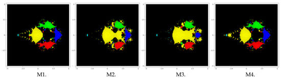
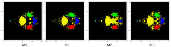
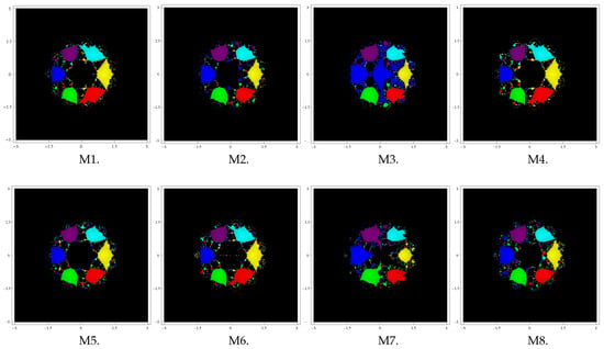
In the first example, we consider the polynomial $P_1\left(z\right)={(z^5-2z^4-2z^3+8z^2-8z)}^2$ which has zeros $\{\pm 2,0,1\pm i\}$ with multiplicity 2. In this case, we use a grid of $500\times 500$ points in a rectangle $D\in \mathbb{C}$ of size $[-3,3]\times [-3,3]$ and assign the colours cyan, green, yellow, red and blue to each initial point in the basin of attraction of zero "$-2$," "$1+i$," "0," "$1-i$" and "2." Basins obtained for the methods M1–M8 are shown in Figure 1, Figure 2 and Figure 3 corresponding to $\beta ={10}^{-2},{10}^{-4},{10}^{-8}$. When observing the behaviour of the methods, we see that the method M5 possesses a lesser number of divergent points, followed by M4 and M6. On the contrary, the methods M3 and M7 have higher numbers of divergent points, followed by M2 and M8. Notice that the basins are becoming wider as parameter β assumes smaller values.

Figure 1. Basins of attraction of M1–M8 for polynomial $P_1\left(z\right)(\beta ={10}^{-2})$.

Figure 2. Basins of attraction of M1–M8 for polynomial $P_1\left(z\right)(\beta ={10}^{-4})$.

Figure 3. Basins of attraction of M1–M8 for polynomial $P_1\left(z\right)(\beta ={10}^{-8})$.

Problem 2.

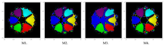
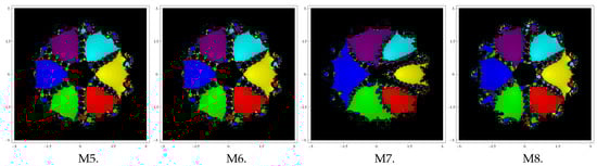
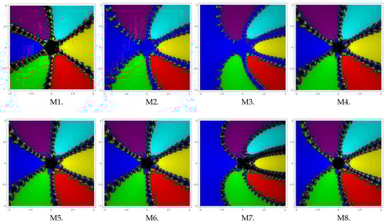
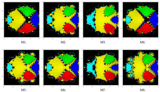
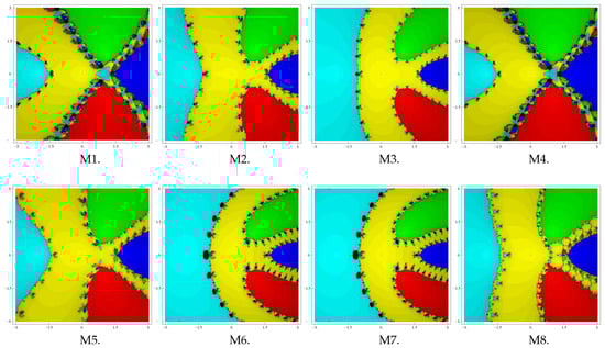
Let us take the polynomial $P_2\left(z\right)={(z^6-1)}^2$ having zeros $\{0,\pm 1\}$ with multiplicity 3. To see the dynamical view, we consider a rectangle $D=[-4,4]\times [-4,4]\in \mathbb{C}$ with $500\times 500$ grid points and allocate the colours colour cyan, green, yellow, red, purple and blue to each initial point in the basins of attraction of zero "$0.5+0.8660i$," "$-0.5-0.8660i$," "1," "$0.5-0.8660i$," "$-0.5+0.8660i$" and "$-1$." Basins for this problem are shown in Figure 4, Figure 5 and Figure 6 corresponding to parameter choices $\beta ={10}^{-2},{10}^{-4},{10}^{-8}$ in the proposed methods. Basins obtained for the methods M1–M8 are shown in Figure 4, Figure 5 and Figure 6 corresponding to $\beta ={10}^{-2},{10}^{-4},{10}^{-8}$. When observing the behaviour of the methods, we see that the methods M3 and M6 possess lesser numbers of divergent points, followed by M1, M4, M8, M2, M3 and M7.

Figure 4. Basins of attraction of M1–M8 for polynomial $P_2\left(z\right)(\beta ={10}^{-2})$.

Figure 5. Basins of attraction of M1–M8 for polynomial $P_2\left(z\right)(\beta ={10}^{-4})$.

Figure 6. Basins of attraction of M1–M8 for polynomial $P_2\left(z\right)(\beta ={10}^{-8})$.

From the graphics, we can judge the behaviour and suitability of any strategy relying upon the conditions. In the event that we pick an underlying point $z_0$ in a zone where various basins of attraction meet one another, it is difficult to foresee which root will be attained by the iterative strategy that starts in $z_0$. Thus, the selection of $z_0$ in such a zone is anything but a decent one. Both the dark zones and the zones with various hues are not appropriate to speculate $z_0$ when we need to accomplish a specific root. The most alluring pictures show up when we have extremely perplexing wildernesses between basins of attraction, and they compare to the situations wherein the strategy is additionally requesting, as it does for the underlying point, and its dynamic conduct is progressively eccentric. We close this segment with a comment that the union conduct of proposed strategies relies on the estimation of parameter $\beta$. The smaller the value of $\beta$, the better the convergence of the technique.

4. Numerical Results

This section is committed to exhibiting the convergence behaviour of the displayed family. In this regard, we consider the special cases of the proposed class, M1–M8 by choosing $(a_1=1/10)$, $(a_2=1/4)$, $(a_3=1/10)$, $(a_4=1/10)$ and $(a_5=1/5)$. Performance is compared with the existing classical Newton modified method (1). We select four test functions for correlation.

To check the theoretical order of convergence, we obtain the computational order of convergence (COC) using the formula (see [25]):

$$COC=\frac{ln|(x_{n+1}-\alpha )/(x_n-\alpha )|}{ln|(x_n-\alpha )/(x_{n-1}-\alpha )|}.$$

All computations were performed in the programming package Mathematica using multiple-precision arithmetic with 4096 significant digits. Numerical results displayed in Table 1, Table 2, Table 3 and Table 4 include: (i) number of iterations $\left(n\right)$ required to converge to the solution such that $|x_{n+1}-x_n|+|f\left(x_n\right)|<{10}^{-100}$, (ii) values of last three consecutive errors $|x_{n+1}-x_n|$, (iii) residual error $\left|f\right(x_n\left)\right|$ and (iv) computational order of convergence (COC).

Example 1

(Eigenvalue problem). One of the challenging tasks in linear algebra is concerned with the Eigenvalues of a large square matrix. Finding the zeros of the characteristic equation of a square matrix of order greater than 4 is another big job. So, we consider the following 9 × 9 matrix.

$$M=\frac{1}{8}\left[\begin{array}{ccccccccc}-12& 0& 0& 19& -19& 76& -19& 18& 437\\ -64& 24& 0& -24& 24& 64& -8& 32& 376\\ -16& 0& 24& 4& -4& 16& -4& 8& 92\\ -40& 0& 0& -10& 50& 40& 2& 20& 242\\ -4& 0& 0& -1& 41& 4& 1& 0& 25\\ -40& 0& 0& 18& -18& 104& -18& 20& 462\\ -84& 0& 0& -29& 29& 84& 21& 42& 501\\ 16& 0& 0& -4& 4& -16& 4& 16& -92\\ 0& 0& 0& 0& 0& 0& 0& 0& 24\end{array}\right].$$

Table 1. Comparison of the performances of methods for Example 1.

Methods	n	$|{\mathit{e}}_{\mathit{n}-2}|$	$|{\mathit{e}}_{\mathit{n}-1}|$	$|{\mathit{e}}_{\mathit{n}}|$	$\mathit{f}\left({\mathit{x}}_{\mathit{n}+1}\right)$	$\mathit{COC}$
MNM	7	$1.70\times {10}^{-21}$	$6.84\times {10}^{-43}$	$1.11\times {10}^{-85}$	$5.90\times {10}^{-681}$	2.000
M1	7	$2.93\times {10}^{-21}$	$2.09\times {10}^{-42}$	$1.07\times {10}^{-84}$	$4.70\times {10}^{-673}$	2.000
M2	7	$3.27\times {10}^{-24}$	$1.87\times {10}^{-48}$	$6.10\times {10}^{-97}$	$1.43\times {10}^{-771}$	2.000
M3	7	$3.66\times {10}^{-23}$	$1.84\times {10}^{-46}$	$4.67\times {10}^{-93}$	$6.47\times {10}^{-741}$	2.000
M4	7	$3.49\times {10}^{-18}$	$4.41\times {10}^{-36}$	$7.04\times {10}^{-72}$	$8.30\times {10}^{-570}$	2.000
M5	6	$6.85\times {10}^{-15}$	$5.28\times {10}^{-30}$	$3.14\times {10}^{-60}$	$1.21\times {10}^{-478}$	2.000
M6	7	$2.03\times {10}^{-21}$	$9.79\times {10}^{-43}$	$2.27\times {10}^{-85}$	$1.82\times {10}^{-678}$	2.000
M7	6	$2.46\times {10}^{-13}$	$8.35\times {10}^{-27}$	$9.60\times {10}^{-54}$	$2.06\times {10}^{-426}$	2.000
M8	7	$6.88\times {10}^{-20}$	$1.36\times {10}^{-39}$	$5.33\times {10}^{-79}$	$3.56\times {10}^{-627}$	2.000

Table 2. Comparison of the performances of methods for Example 2.

Methods	n	$|{\mathit{e}}_{\mathit{n}-2}|$	$|{\mathit{e}}_{\mathit{n}-1}|$	$|{\mathit{e}}_{\mathit{n}}|$	$\mathit{f}\left({\mathit{x}}_{\mathit{n}+1}\right)$	$\mathit{COC}$
MNM	7	$1.61\times {10}^{-20}$	$6.51\times {10}^{-41}$	$1.06\times {10}^{-81}$	$1.86\times {10}^{-324}$	2.000
M1	7	$3.60\times {10}^{-21}$	$2.94\times {10}^{-41}$	$1.95\times {10}^{-84}$	$1.77\times {10}^{-335}$	2.000
M2	7	$7.50\times {10}^{-18}$	$2.11\times {10}^{-35}$	$1.68\times {10}^{-70}$	$2.71\times {10}^{-279}$	2.000
M3	7	$2.63\times {10}^{-18}$	$2.44\times {10}^{-36}$	$2.08\times {10}^{-72}$	$5.58\times {10}^{-287}$	2.000
M4	6	$1.85\times {10}^{-22}$	$4.10\times {10}^{-47}$	$2.02\times {10}^{-96}$	$5.76\times {10}^{-388}$	2.000
M5	7	$6.66\times {10}^{-16}$	$2.23\times {10}^{-31}$	$2.48\times {10}^{-62}$	$2.30\times {10}^{-246}$	2.000
M6	7	$1.30\times {10}^{-20}$	$4.26\times {10}^{-41}$	$4.57\times {10}^{-82}$	$6.60\times {10}^{-326}$	2.000
M7	7	$1.41\times {10}^{-17}$	$7.79\times {10}^{-35}$	$2.38\times {10}^{-69}$	$1.19\times {10}^{-274}$	2.000
M8	6	$1.16\times {10}^{-17}$	$6.61\times {10}^{-36}$	$2.13\times {10}^{-72}$	$1.18\times {10}^{-288}$	2.000

Table 3. Comparison of the performances of methods for Example 3.

Methods	n	$|{\mathit{e}}_{\mathit{n}-2}|$	$|{\mathit{e}}_{\mathit{n}-1}|$	$|{\mathit{e}}_{\mathit{n}}|$	$\mathit{f}\left({\mathit{x}}_{\mathit{n}+1}\right)$	$\mathit{COC}$
MNM	9	$3.65\times {10}^{-12}$	$2.22\times {10}^{-22}$	$8.24\times {10}^{-43}$	$3.84\times {10}^{-168}$	2.000
M1	9	$2.99\times {10}^{-12}$	$1.49\times {10}^{-22}$	$3.70\times {10}^{-43}$	$1.55\times {10}^{-169}$	2.000
M2	9	$9.51\times {10}^{-12}$	$1.52\times {10}^{-21}$	$3.88\times {10}^{-41}$	$1.92\times {10}^{-161}$	2.000
M3	9	$7.90\times {10}^{-12}$	$1.05\times {10}^{-21}$	$1.84\times {10}^{-41}$	$9.58\times {10}^{-163}$	2.000
M4	9	$4.35\times {10}^{-13}$	$3.11\times {10}^{-24}$	$1.59\times {10}^{-46}$	$5.18\times {10}^{-183}$	2.000
M5	9	$2.28\times {10}^{-11}$	$8.82\times {10}^{-21}$	$1.32\times {10}^{-39}$	$2.58\times {10}^{-155}$	2.000
M6	9	$3.81\times {10}^{-12}$	$2.42\times {10}^{-22}$	$9.74\times {10}^{-43}$	$7.49\times {10}^{-168}$	2.000
M7	9	$1.08\times {10}^{-11}$	$1.95\times {10}^{-21}$	$6.42\times {10}^{-41}$	$1.44\times {10}^{-160}$	2.000
M8	9	$7.78\times {10}^{-16}$	$1.01\times {10}^{-29}$	$1.69\times {10}^{-57}$	$6.83\times {10}^{-227}$	2.000

Table 4. Comparison of the performances of methods for Example 4.

Methods	n	$|{\mathit{e}}_{\mathit{n}-2}|$	$|{\mathit{e}}_{\mathit{n}-1}|$	$|{\mathit{e}}_{\mathit{n}}|$	$\mathit{f}\left({\mathit{x}}_{\mathit{n}+1}\right)$	$\mathit{COC}$
MNM	7	$2.87\times {10}^{-15}$	$2.75\times {10}^{-30}$	$2.51\times {10}^{-60}$	$5.82\times {10}^{-478}$	2.000
M1	7	$2.88\times {10}^{-15}$	$2.77\times {10}^{-30}$	$2.55\times {10}^{-60}$	$6.58\times {10}^{-478}$	2.000
M2	7	$3.42\times {10}^{-15}$	$3.97\times {10}^{-30}$	$5.34\times {10}^{-60}$	$2.59\times {10}^{-475}$	2.000
M3	7	$4.44\times {10}^{-15}$	$6.86\times {10}^{-30}$	$1.64\times {10}^{-59}$	$2.27\times {10}^{-471}$	2.000
M4	7	$5.71\times {10}^{-15}$	$1.16\times {10}^{-29}$	$4.78\times {10}^{-59}$	$1.30\times {10}^{-467}$	2.000
M5	7	$5.49\times {10}^{-15}$	$1.07\times {10}^{-29}$	$4.09\times {10}^{-59}$	$3.73\times {10}^{-468}$	2.000
M6	7	$2.99\times {10}^{-15}$	$2.99\times {10}^{-30}$	$2.97\times {10}^{-60}$	$2.22\times {10}^{-477}$	2.000
M7	7	$4.48\times {10}^{-15}$	$6.99\times {10}^{-30}$	$1.70\times {10}^{-59}$	$3.07\times {10}^{-471}$	2.000
M8	7	$3.37\times {10}^{-15}$	$3.83\times {10}^{-30}$	$4.94\times {10}^{-60}$	$1.37\times {10}^{-475}$	2.000

The characteristic polynomial of the matrix $\left(M\right)$ is given as

$$\begin{array}{cc}\hfill f_1\left(x\right)=& x^9-29x^8+349x^7-2261x^6+8455x^5-17663x^4+15927x^3\hfill \\ \hfill & +6993x^2-24732x+12960.\hfill \end{array}$$

This function has one multiple zero $\alpha =3$ with multiplicity 4. We choose initial approximations $x_0=2.75$ and obtain the numerical results as shown in Table 1.

Example 2

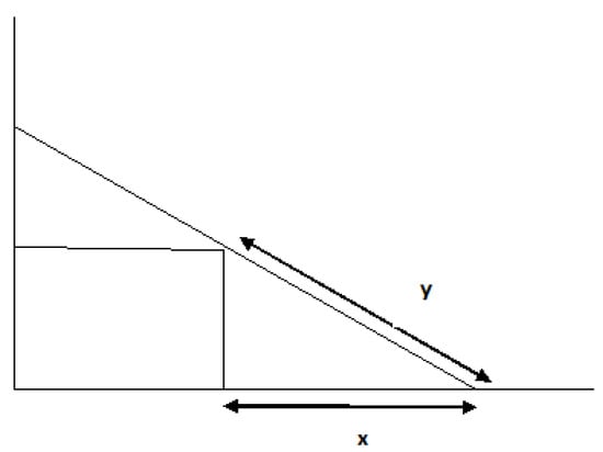
(Beam Designing Model). We consider a beam positioning problem (see [26]) where a beam of length r unit is leaning against the edge of a cubical box with sides of length 1 unit each, such that one end of the beam touches the wall and the other end touches the floor, as shown in Figure 7.

Figure 7. Beam positioning problem.

The problem is: What should be the distance along the floor from the base of the wall to the bottom of the beam? Suppose y is the distance along the beam from the floor to the edge of the box, and let x be the distance from the bottom of the box to bottom of the beam. Then, for a given value of r, we have

$$x^4+4x^3-24x^2+16x+16=0.$$

The positive solution of the equation is a double root $x=2$. We consider the initial guess $x_0=1.8$ to find the root. Numerical results of various methods are shown in Table 2.

Example 3.

The van der Waals equation of state, whose expression is

$$\left(P+\frac{a_1{n}^2}{V^2}\right)(V-n{a}_2)=nRT,$$

explains the behaviour of a real gas by taking in the ideal gas equations two more parameters, $a_1$ and $a_2$, specific for each gas. In order to determine the volume V of the gas in terms of the remaining parameters, we are required to solve the nonlinear equation in V.

$$P{V}^3-(n{a}_{2}P+nRT)V^2+a_1{n}^{2}V-a_1{a}_2{n}^3=0.$$

Given the constants $a_1$ and $a_2$ of a particular gas, one can find values for n, P and T, such that this equation has three real roots. By using the particular values, we obtain the following nonlinear function

$$f1\left(x\right)=x^3-5.22x^2+9.0825x-5.2675,$$

having three roots, out of which one is a multiple zero $\alpha =1.75$ of multiplicity of order two, and other one is simple zero $\xi =1.72$. However, we seek the multiple zero $\alpha =1.75$. We consider initial guess $x_0=1.8$ to obtain this zero. The numerical results so-obtained are shown in Table 3.

Example 4.

Lastly, consider the test function

$$f_4\left(x\right)=\left(x^2+1\right)\left(2x{e}^{x^2+1}+x^3-x\right){cosh}^2\left(\frac{\pi x}{2}\right).$$

The function has multiple zero $\alpha =i$ of multiplicity 4. We chose the initial approximation $x_0=1.25i,$ for obtaining the zero of the function. Numerical results of various methods are shown in Table 4.

5. Conclusions

In the foregoing work, we have developed a class of optimal second order methods free from derivatives for solving nonlinear uni-variate functions. Convergence analysis has shown the second order convergence under standard presumptions with respect to the nonlinear functions whose zeros we were searching for. Some best cases of the class were discussed. Their stability was tested by analyzing complex geometry shown by drawing their basins. We have noticed from the graphics that the basins become wider and wider as the parameter assumes smaller values. The methods were employed to solve some nonlinear uni-variate equations and also compared with already defined techniques. We conclude the paper with the remark that derivative-free techniques may prove to be good options for Newton-like methods in the cases where derivatives are expensive to evaluate.

References

- Argyros, I.K. Convergence and Applications of Newton-Type Iterations; Spring: New York, NY, USA, 2008. [Google Scholar]
- Hoffman, J.D. Numerical Methods for Engineers and Scientists; McGraw-Hill Book Company: New York, NY, USA, 1992. [Google Scholar]
- Schröder, E. Über unendlich viele Algorithmen zur Auflösung der Gleichungen. Math Ann. 1870, 2, 317–365. [Google Scholar] [CrossRef]
- Kumar, D.; Sharma, J.R.; Cesarano, C. One-point optimal family of multiple root solvers of second-Order. Mathematics 2019, 7, 655. [Google Scholar] [CrossRef]
- Dong, C. A family of multipoint iterative functions for finding multiple roots of equations. Int. J. Comput. Math. 1987, 21, 363–367. [Google Scholar] [CrossRef]
- Geum, Y.H.; Kim, Y.I.; Neta, B. A class of two-point sixth-order multiple-zero finders of modified double-Newton type and their dynamics. Appl. Math. Comput. 2015, 70, 387–400. [Google Scholar] [CrossRef]
- Hansen, E.; Patrick, M. A family of root finding methods. Numer. Math. 1977, 27, 257–269. [Google Scholar] [CrossRef]
- Kansal, M.; Kanwar, V.; Bhatia, S. On some optimal multiple root-finding methods and their dynamics. Appl. Appl. Math. 2015, 10, 349–367. [Google Scholar]
- Li, S.G.; Cheng, L.Z.; Neta, B. Some fourth-order nonlinear solvers with closed formulae for multiple roots. Comput. Math. Appl. 2010, 59, 126–135. [Google Scholar] [CrossRef]
- Li, S.; Liao, X.; Cheng, L. A new fourth-order iterative method for finding multiple roots of nonlinear equations. Appl. Math. Comput. 2009, 215, 1288–1292. [Google Scholar]
- Lotfi, T.; Sharifi, S.; Salimi, M.; Siegmund, S. A new class of three-point methods with optimal convergence order eight and its dynamics. Numer. Algor. 2015, 68, 261–288. [Google Scholar] [CrossRef]
- Neta, B. New third order nonlinear solvers for multiple roots. Appl. Math. Comput. 2008, 202, 162–170. [Google Scholar] [CrossRef]
- Osada, N. An optimal multiple root-finding method of order three. J. Comput. Appl. Math. 1994, 51, 131–133. [Google Scholar] [CrossRef]
- Sharifi, M.; Babajee, D.K.R.; Soleymani, F. Finding the solution of nonlinear equations by a class of optimal methods. Comput. Math. Appl. 2012, 63, 764–774. [Google Scholar] [CrossRef]
- Sharma, J.R.; Sharma, R. Modified Jarratt method for computing multiple roots. Appl. Math. Comput. 2010, 217, 878–881. [Google Scholar] [CrossRef]
- Soleymani, F.; Babajee, D.K.R.; Lotfi, T. On a numerical technique for finding multiple zeros and its dynamics. J. Egypt. Math. Soc. 2013, 21, 346–353. [Google Scholar] [CrossRef]
- Victory, H.D.; Neta, B. A higher order method for multiple zeros of nonlinear functions. Int. J. Comput. Math. 1983, 12, 329–335. [Google Scholar] [CrossRef]
- Yun, B.I. A non-iterative method for solving non-linear equations. Appl. Math. Comput. 2008, 198, 691–699. [Google Scholar] [CrossRef]
- Zhou, X.; Chen, X.; Song, Y. Constructing higher-order methods for obtaining the multiple roots of nonlinear equations. J. Comput. Appl. Math. 2011, 235, 4199–4206. [Google Scholar] [CrossRef]
- Kung, H.T.; Traub, J.F. Optimal order of one-point and multipoint iteration. J. Assoc. Comput. Mach. 1974, 21, 643–651. [Google Scholar] [CrossRef]
- Traub, J.F. Iterative Methods for the Solution of Equations; Chelsea Publishing Company: New York, NY, USA, 1982. [Google Scholar]
- Vrscay, E.R.; Gilbert, W.J. Extraneous fixed points, basin boundaries and chaotic dynamics for Schröder and König rational iteration functions. Numer. Math. 1988, 52, 1–16. [Google Scholar] [CrossRef]
- Scott, M.; Neta, B.; Chun, C. Basin attractors for various methods. Appl. Math. Comput. 2011, 218, 2584–2599. [Google Scholar] [CrossRef]
- Varona, J.L. Graphic and numerical comparison between iterative methods. Math. Intell. 2002, 24, 37–46. [Google Scholar] [CrossRef]
- Weerakoon, S.; Fernando, T.G.I. A variant of Newton’s method with accelerated third-order convergence. Appl. Math. Lett. 2000, 13, 87–93. [Google Scholar] [CrossRef]
- Zachary, J.L. Introduction to Scientific Programming: Computational Problem Solving Using Maple and C; Springer: New York, NY, USA, 2012. [Google Scholar]
© 2020 by the authors. Licensee MDPI, Basel, Switzerland. This article is an open access article distributed under the terms and conditions of the Creative Commons Attribution (CC BY) license (http://creativecommons.org/licenses/by/4.0/).