A Multilevel Iteration Method for Solving a Coupled Integral Equation Model in Image Restoration

Abstract

The problem of out-of-focus image restoration can be modeled as an ill-posed integral equation, which can be regularized as a second kind of equation using the Tikhonov method. The multiscale collocation method with the compression strategy has already been developed to discretize this well-posed equation. However, the integral computation and solution of the large multiscale collocation integral equation are two time-consuming processes. To overcome these difficulties, we propose a fully discrete multiscale collocation method using an integral approximation strategy to compute the integral, which efficiently converts the integral operation to the matrix operation and reduces costs. In addition, we also propose a multilevel iteration method (MIM) to solve the fully discrete integral equation obtained from the integral approximation strategy. Herein, the stopping criterion and the computation complexity that correspond to the MIM are shown. Furthermore, a posteriori parameter choice strategy is developed for this method, and the final convergence order is evaluated. We present three numerical experiments to display the performance and computation efficiency of our proposed methods.

1. Introduction

Continuous integral equations are often used to model certain practical problems in image processing. However, the corresponding discrete models are often used instead of continuous models because discrete models are much easier and more convenient to implement than continuous integral models. Discrete models are piecewise constant approximations of integral equation models, and they introduce a bottleneck model error that cannot be addressed by any image processing method. To overcome the accuracy deficiency of conventional discrete reconstruction models, we use continuous models directly to restore images, which are more in line with physical laws. This idea first appeared in [1], and was widely used later, such as in [2,3,4]. In addition to making more sense in physics, continuous models can be discretized with higher-order accuracy. This means that the model error will be significantly decreased when compared with piecewise constant discretization, especially in the field of image enlargement.

Many researchers have made great contributions to the solution of integral equations, however, many difficulties remain. First, integral operators are compact in Banach space since integral kernels are normally smooth. This will produce a situation in which the solutions of the relevant integral equations do not depend on the known data continuously. To overcome this problem, the Tikhonov [5] and the Lavrentiev [6] regularization methods were proposed to regularize the ill-posed integral equation into a second-kind integral equation. Second, the equation using the Tikhonov regularization method contains a composition integral operator, which greatly increases the computation time. Given this condition, a coupled system equation that only involves a one-time integral operator was proposed in [7] to reduce the high computational cost. The original second-kind integral equation involves the composition of an integral operator, which is time-consuming. The collocation method [8] and the Galerkin method [9] were proposed to discretize the coupled system, and the collocation method is much easier. The third problem is that after the coupled system equation is discretized by the collocation method, a full coefficient matrix is generated. To overcome this issue, Chen et al. [10] proposed that the integral operator be represented using a multiscale basis and obtained a sparse coefficient matrix. Then, a matrix compression technique [1,11] is used to approximate that matrix, which does not affect the existing convergence order. Finally, appropriately choosing the regularization parameter (see [12,13,14,15,16,17]) is a crucial process that should balance between the approximation accuracy and the well-posedness.

The purpose of this paper is to efficiently solve the second-kind integral equation on the basis of the previous achievements of other researchers. Although the equivalent coupled system is developed to reduce the computational complexity caused by the composition of the original integral operator, this is insufficient because a lot of computing time is required to compute the integral. Therefore, inspired by [18], we further propose a fully discrete multiscale collocation method using an integral approximation strategy to compute the integration. The idea of this strategy is the use of the Gaussian quadrature formula to efficiently compute the sparse coefficient matrix. By using the piecewise Gauss-Legendre quadrature, we turn the calculation of the integration into the matrix operation, which will tremendously reduce the computation time. Another challenging issue is that directly solving the large, fully discrete system obtained from the matrix compression strategy is time-consuming. Inspired by [19], we propose a multilevel iteration method (MIM) to solve the large, fully discrete coupled system, and we further present the computation complexity of the MIM. We also propose a stopping criterion of this iteration process, and we prove that this criterion can maintain the existing convergence rate. Finally, we adopt an a posteriori choice of the regularization parameter related to the MIM and then show that it will lead to an optimal convergence order.

This paper is organized into six sections. In Section 2, an overview flowchart is displayed first, and then the integral equation model of the first kind is reviewed to reconstruct an out-of-focus image. Following this, an equivalent coupled system is deduced. In Section 3, we present the fast multiscale collocation method to discretize the coupled system using piecewise polynomial spaces. Additionally, a compression strategy is developed to generate a sparse coefficient matrix in order to make the coupled equation easily solvable. Finally, we propose an integral approximation strategy to compute the nonzero entries of the compressed coefficient matrix, which turns the operation of the integral into a matrix computation. We also provide a convergence analysis of the proposed method. In Section 4, we propose a multilevel iteration method corresponding to the multiscale method to solve the integral equations, and a complete analysis of the convergence rate of the corresponding approximate solution is shown. A posteriori choice of the regularization parameter, which is related to the multilevel iteration method, is presented in Section 5, and we further prove that the MIM, combined with this posteriori parameter choice, makes our solution optimal. In Section 6, we report three comparative tests to verify the efficiency of our two proposed methods. The first test shows the computing efficiency of the coefficient matrix using the integral approximation strategy and the numerical quadrature scheme in [1]. The other two tests exhibit the performance of the MIM compared with the Gaussian elimination method and the multilevel augmentation method, respectively. These tests reveal the high efficiency of our proposed methods.

2. The Integral Equation Model for Image Restoration

In this section, we first depict the overall process of reconstructing out-of-focus images and then describe some common notations that are used throughout the paper. Finally, in the second subsection, we introduce the approach to formulating our image restoration problem into an integral equation.

2.1. System Overview

We present an overview flowchart for reconstructing an out-of-focus image in Figure 1. This process includes four main parts, that is, modeling, discretization, the parameter choice rule, and solving the equation.

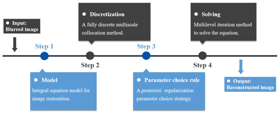
Figure 1. Overview flowchart.

For the input out-of-focus image, we formulate it into a Tikhonov-regularized integral equation, which is described in the next subsection. Solving this integral equation necessitates discretization. We propose a fully discrete multiscale collocation method based on an integral approximation strategy. This method works by converting the calculation of the integral into a matrix operation. The next two parts describe the parameter choice rule and solution of the problem. We note that these two parts are actually a whole when executed in practice. However, we describe it in two parts because it is too complicated to describe as a whole. For a clearer presentation, we first display the multilevel iteration method in Section 4 under the condition that we have already selected a good regularization parameter. Then, we describe how this regularization parameter is chosen in Section 5.

Some notations are needed. Suppose that $R^d$ represents d-dimensional Euclidean space. In addition, $\Omega \subset R^2$ and $E\subset R$ denote the subsets of $R^d$. $L^{\infty }$ is a special kind of space of $L^p$ when $p=\infty$, and it is proved to be a Banach space. We use x, including x with upper and lower indices, to denote the solution of the equation. Similarly, we use y, including y with upper and lower indices, to denote the known variable of the equation. Furthermore, the operator $\mathcal{K}$ represents the blurring kernel, and ${\mathcal{K}}^{*}$ represents the adjoint operator of $\mathcal{K}$. The notation $A{\oplus }^{\perp }B$ denotes the direct sum of spaces A and B when $A\perp B$. The notation $a\sim b$ means that a and b are in the same order. $\mathcal{R}(·)$ represents the range of the operator. Finally, many extended and new notations that are not declared here are defined in the context in which they are first used.

2.2. Model Definition

In this subsection, we describe an integral equation model obtained from a reformulation of the Tikhonov regularization equation for image restoration. In addition, an equivalent coupled system is developed for solving this integral equation quickly and efficiently.

Assume that the whole image is a support set. In general, images are usually rectangular. Let $\Omega \subset R^2$ denotes the image domain, also the support set. The image restoration can be modeled by a continuous integral equation of the first kind

$$\mathcal{K}x=y,$$

(1)

where y is the blurred image and we aim to reconstruct the blurred image y into a clearer image $x:\Omega \to R$. Thus, image x can also be called the reconstructed image. $\mathcal{K}$ is the linear compact operator defined in terms of a kernel g by

$$(\mathcal{K}x)(\mathbf{u}):={\int }_{\Omega }g(\mathbf{u},{\mathbf{u}}^{\prime })x({\mathbf{u}}^{\prime })d{\mathbf{u}}^{\prime },\mathbf{u}\in \Omega .$$

(2)

Let $\Omega =E\times E$, with $E:=[0,1]$. The images may not be in $[0,1]\times [0,1]$, but can be shaped to by scaling and shifting. According to [20], the out-of-focus image is usually modeled with the kernel

$$g(\mathbf{u},{\mathbf{u}}^{\prime })=\frac{1}{2\pi {\sigma }^2}exp(-\frac{{(u-u^{\prime })}^2+{(v-v^{\prime })}^2}{2{\sigma }^2}),$$

(3)

where $\mathbf{u}$$:=(u,v)$,${\mathbf{u}}^{\prime }$$:=(u^{\prime },v^{\prime })\in \Omega$, and $\sigma$ is the parameter characterizing the level of ambiguity in the kernel.

Blurring kernel (3) is a two-dimensional symmetric operator. It can be written as a combination of two univariate integral operators. That is to say, solving Equation (1) is equivalent to solving the following system:

$$\begin{array}{c}\hfill \frac{1}{\sqrt{2\pi }\sigma }{\int }_0^{1}exp(-\frac{{(v-v^{\prime })}^2}{2{\sigma }^2})x_1(u,v^{\prime })d{v}^{\prime }=y(u,v),\\ \hfill \frac{1}{\sqrt{2\pi }\sigma }{\int }_0^{1}exp(-\frac{{(u-u^{\prime })}^2}{2{\sigma }^2})x_2(u^{\prime },v^{\prime })d{u}^{\prime }=x_1(u,v^{\prime }).\end{array}$$

(4)

In this system, $x_2$ is the final solution of the reconstruction, and $x_1$ is the intermediate result. These two equations mean that we can first deal with all the rows of the image (first equation) and then all the columns (second equation). Hence, the problem has changed significantly. We have changed the procedure of dealing with a two-dimensional image to processing the rows of the image first, and then the columns. Furthermore, as can be seen from the two equations in (4), the rows and columns of the image are processed similarly, and both processes can be formulated to a one-dimensional integral equation:

$$\mathcal{K}x=y.$$

(5)

For $x\in X:=L^{\infty }(E)$, $\mathcal{K}$ is the linear compact operator defined by

$$\mathcal{K}x(u):={\int }_{E}k(u,u^{\prime })x(u^{\prime })d{u}^{\prime },u\in E,$$

with

$$k(u,u^{\prime })=\frac{1}{\sqrt{2\pi }\sigma }exp(-\frac{{(u-u^{\prime })}^2}{2{\sigma }^2}),u,u^{\prime }\in E,$$

and $y\in X$ is the observed function. Hence, we focus on Equation (5) in the following illustration.

Ill-posedness makes Equation (5) difficult to solve, but the Tikhonov regularization method can handle this problem. By using the Tikhonov regularization method, we get the following equation:

$$(\alpha I+{\mathcal{K}}^{*}\mathcal{K})x_{\alpha }={\mathcal{K}}^{*}y$$

(6)

where $\alpha >0$ is the regularization parameter, and ${\mathcal{K}}^{*}$ is the adjoint operator of $\mathcal{K}$. It is easy to prove that the operator $\alpha I+{\mathcal{K}}^{*}\mathcal{K}$ is invertible. In addition, $y^{\delta }$ is usually noisy data, with

$$\parallel y-y^{\delta }{\parallel }_{\infty }\le \delta$$

(7)

for a noise level $\delta$. $x_{\alpha }^{\delta }$ denotes the solution of Equation (6) when y is replaced by $y^{\delta }$. $\mathcal{K}$ is self-adjoint; that is, ${\mathcal{K}}^{*}=\mathcal{K}$. Note that Equation (6) includes ${\mathcal{K}}^{*}\mathcal{K}$, which is defined by a 2-fold integral. This 2-fold integral is tremendously computationally expensive. By letting $v_{\alpha }^{\delta }:=\frac{y^{\delta }-\mathcal{K}{x}_{\alpha }^{\delta }}{\sqrt{\alpha }}$, the authors of [7] split Equation (6) into a coupled system:

$$\left\{\begin{array}{c}\sqrt{\alpha }{x}_{\alpha }^{\delta }-{\mathcal{K}}^{*}{v}_{\alpha }^{\delta }=0\hfill \\ \mathcal{K}{x}_{\alpha }^{\delta }+\sqrt{\alpha }{v}_{\alpha }^{\delta }=y^{\delta }\hfill \end{array}.\right.$$

(8)

These two were proven to be equal in [7], and the advantage is that system (8) only involves one single integral. Thus, we do not solve Equation (6) but instead solve system (8) to reduce the computational difficulties.

In the next section, we apply a fully discrete method to solve system (8).

3. Fully Discrete Multiscale Collocation Method

In this section, a multiscale method is reviewed first, and then we develop a fully discrete formulation of the multiscale collocation method using an integral approximation strategy. By using this strategy, we turn the computation of the integral into a matrix operation, which will greatly reduce the calculation time.

3.1. Multiscale Collocation Method

Let us begin with a quick review of the fast collocation method [10,21,22,23,24] for solving system (8).

We denote $\mathbb{N}$ as the natural numbers set. For $n\in {\mathbb{N}}_{+},{\mathbb{N}}_{+}:=\mathbb{N}\backslash 0$, let ${\mathbb{Z}}_n:=\{0,1,2,\dots ,n-1\}$. Let ${\mathbb{X}}_n,n\in \mathbb{N}$, denote the subspaces of $L^{\infty }(E)$. Let ${\mathbb{W}}_0:={\mathbb{X}}_0,{\mathbb{X}}_{n+1}={\mathbb{X}}_n{\oplus }^{\perp }{\mathbb{W}}_{n+1},n\in \mathbb{N}$. More clearly,

$${\mathbb{X}}_n={\mathbb{W}}_0{\oplus }^{\perp }{\mathbb{W}}_1{\oplus }^{\perp }\cdots {\oplus }^{\perp }{\mathbb{W}}_n.$$

A basis construction of ${\mathbb{X}}_n$ can be found in [25,26]. Suppose that $\{e_{ij}\}$ is an orthogonal basis of ${\mathbb{W}}_i$. Let ${\mathbb{U}}_n:=\{(i,j):i\in {\mathbb{Z}}_{n+1},j\in {\mathbb{Z}}_{w(i)}\}$, where $w(n)$ is the dimension of ${\mathbb{W}}_n$. According to (9), we get

$${\mathbb{X}}_n=\mathrm{span}\{e_{ij}:(i,j)\in {\mathbb{U}}_n\}.$$

Similarly, the multiscale collocation functionals and the collocation points are important. Suppose that ${\ell }_{ij}$ is the collocation functional. Meanwhile, we have a sequence of collocation points $\{v_{ij}:(i,j)\in U_n\}$ in E. We define an interpolation projection $P_n:L^{\infty }(E)\to {\mathbb{X}}_n,n\in \mathbb{N}$ and an orthogonal projection $Q_n:L^2(E)\to {\mathbb{X}}_n,n\in \mathbb{N}$.

For $n\in N$, let ${\mathcal{K}}_n:=P_n{\mathcal{K}|}_{{\mathbb{X}}_n}$. The multiscale collocation method for system (8) is to find the solutions

$v_{\alpha ,n}^{\delta }:={\displaystyle \sum _{(i,j)\in U_n}}{v}_{ij}^{\alpha ,n}{e}_{ij}$ and $x_{\alpha ,n}^{\delta }:={\displaystyle \sum _{(i,j)\in U_n}}{x}_{ij}^{\alpha ,n}{e}_{ij}$ of the system

$$\left\{\begin{array}{c}\sqrt{\alpha }{x}_{\alpha ,n}^{\delta }-{\mathcal{K}}_n^{*}{v}_{\alpha ,n}^{\delta }=0\hfill \\ {\mathcal{K}}_n{x}_{\alpha ,n}^{\delta }+\sqrt{\alpha }{v}_{\alpha ,n}^{\delta }=P_n{y}^{\delta }\hfill \end{array}.\right.$$

(9)

For $(i,j),(i^{\prime }{j}^{\prime })\in U_n$, after the introduction of three definitions,

$$\begin{array}{c}\hfill {\mathbf{E}}_n:=[⟨{\ell }_{i^{\prime }{j}^{\prime }},e_{ij}⟩],{\mathbf{K}}_n:=[⟨{\ell }_{i^{\prime }{j}^{\prime }},\mathcal{K}{e}_{ij}⟩],{\mathbf{y}}_n^{\delta }:=[⟨{\ell }_{i^{\prime }{j}^{\prime }},y^{\delta }⟩],\end{array}$$

Equation (9) has the matrix form

$$\left[\begin{array}{cc}\sqrt{\alpha }{\mathbf{E}}_n& -{\mathbf{K}}_n\\ {\mathbf{K}}_n& \sqrt{\alpha }{\mathbf{E}}_n\end{array}\right]\left[\begin{array}{c}{\mathbf{x}}_{\alpha ,n}^{\delta }\\ {\mathbf{v}}_{\alpha ,n}^{\delta }\end{array}\right]=\left[\begin{array}{c}\mathbf{0}\\ {\mathbf{y}}_n^{\delta }\end{array}\right].$$

(10)

Note that ${\mathbf{K}}_n$ is a dense matrix. The compression of ${\mathbf{K}}_n$ is an important factor of our method. Following the compression strategy of [7], we get the compression matrix ${\overline{\mathbf{K}}}_n$:

$${\overline{\mathbf{K}}}_n=\left\{\begin{array}{c}⟨{\ell }_{ij},\mathcal{K}{e}_{i^{\prime }{j}^{\prime }}⟩,i+i^{\prime }\le n,\hfill \\ 0,otherwise.\hfill \end{array}\right.$$

Thus, substituting ${\mathbf{K}}_n$ with ${\overline{\mathbf{K}}}_n$, we finally need to solve the equation

$$\left[\begin{array}{cc}\sqrt{\alpha }{\mathbf{E}}_n& -{\overline{\mathbf{K}}}_n\\ {\overline{\mathbf{K}}}_n& \sqrt{\alpha }{\mathbf{E}}_n\end{array}\right]\left[\begin{array}{c}{\mathbf{x}}_{\alpha ,n}^{\delta }\\ {\mathbf{v}}_{\alpha ,n}^{\delta }\end{array}\right]=\left[\begin{array}{c}\mathbf{0}\\ {\mathbf{y}}_n^{\delta }\end{array}\right].$$

(11)

3.2. Integral Approximation Strategy

The computation of system (11) mainly lies in the integral operator ${\mathcal{K}}_n$. Next, we focus on this problem and develop an integral approximation strategy using the Gaussian quadrature formula to solve this coupled system.

Note that the integral operator $\mathcal{K}$ is

$$\mathcal{K}{e}_{ij}(u)={\int }_{E}k(u,u^{\prime })e_{ij}(u)d{u}^{\prime },$$

and the orthogonal basis functions $\{e_{ij}:(i,j)\in U_n\}$ are all piecewise polynomial functions. Thus, the piecewise Gauss–Legendre quadrature is used here.

Integral approximation strategy: With the supports of these basis functions, we divide E equally into ${\mu }^n$ parts. Let $E_q:=[\frac{q}{{\mu }^n},\frac{q+1}{{\mu }^n}]$, for $q\in {\mathbb{Z}}_{{\mu }^n}$; then, $E={\bigcup }_{q\in {\mathbb{Z}}_{{\mu }^n}}{E}_q$. Each basis function is a continuous function in $E_q,q\in {\mathbb{Z}}_{{\mu }^n}$. Then, we choose $m>1$ Gaussian points in each part $E_q$ and let $\gamma =2m-1$. All Gaussian points form a set of piecewise Gaussian points G in order. Let $g(n):=\left|G\right|$; then, $g(n)=m\times {\mu }^n$. Thus, the integral under the accuracy of $\gamma$ in $E_q$ can be written as

$$\mathcal{K}{e}_{ij}{(u)|}_{E_q}\approx \sum _{t=qm+1}^{(q+1)m}{\rho }_{t}k(u,g_t)e_{ij}(g_t),u\in E_q,$$

(12)

where $\{g_t,t=qm+1,\cdots ,(q+1)m\}$ represents a Gaussian point in $E_q$, and ${\rho }_t$ represents the weight corresponding to $g_t$. Further, the integral with an accuracy of $\gamma$ in E is

$$\mathcal{K}{e}_{ij}(u){|}_E\approx \sum _{q\in {\mathbb{Z}}_{{\mu }^n}}\mathcal{K}{e}_{ij}(u){|}_{E_q},$$

which can be written as a formulation of vector multiplication

$$\mathcal{K}{e}_{ij}(u){{|}_E\approx [k(u,g_1),k(u,g_2),\dots ,k(u,g_{g(n)})][w_{ij}(g_1),w_{ij}(g_2),\dots ,w_{ij}(g_{g(n)}))]}^T.$$

Furthermore, as shown in Figure 2, we can use this strategy to approximate ${\mathbf{K}}_n$ as a matrix form of

$${\mathbf{K}}_n\approx L_n{K}_{s(n)\times g(n)}{W}_{g(n)\times s(n)},$$

(13)

where $W_{g(n)\times s(n)}$ is a basis function matrix with weights. And it stands for all the basis functions $\{e_{ij},(i,j)\in U_n\}$ act on all piecewise Gaussian points of G with the weight of ${\rho }_t$. $L_n$ denotes the matrix representation of point evaluation functional ${\ell }_s$, and the details of $L_n$ refer to [26].

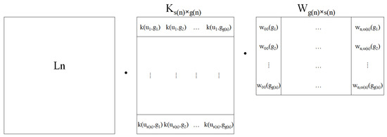
Figure 2. The components of matrix ${\mathbf{K}}_n$.

In order to combine it with the matrix compression strategy, we write Equation (13) in blocks. This is the matrix representation ${\tilde{\mathbf{K}}}_n,i,i^{\prime }\in {\mathbb{Z}}_{n+1}$, which is the approximate value of ${\overline{\mathbf{K}}}_n$ using the integral approximation strategy.

$${\tilde{\mathbf{K}}}_n=\left\{\begin{array}{c}{(L_n{K}_{s(n)\times g(n)}{W}_{g(n)\times s(n)})}_{i{i}^{\prime }},i+i^{\prime }\le n\hfill \\ 0,otherwise\hfill \end{array}\right.$$

(14)

Then, Equation (10) becomes a formulation of the fully discrete multiscale collocation equation:

$$\left[\begin{array}{cc}\sqrt{\alpha }{\mathbf{E}}_n& -{\tilde{\mathbf{K}}}_n\\ {\tilde{\mathbf{K}}}_n& \sqrt{\alpha }{\mathbf{E}}_n\end{array}\right]\left[\begin{array}{c}{\mathbf{x}}_{\alpha ,n}^{\delta }\\ {\mathbf{v}}_{\alpha ,n}^{\delta }\end{array}\right]=\left[\begin{array}{c}\mathbf{0}\\ {\mathbf{y}}_n^{\delta }\end{array}\right],$$

(15)

where ${\tilde{\mathbf{K}}}_n$ is as given in Equation (14).

Let $\mathcal{A}:={\mathcal{K}}^{*}\mathcal{K}$, ${\mathcal{A}}_n:={\mathcal{K}}_n^{*}{\mathcal{K}}_n$. Assume that ${\overline{\mathcal{K}}}_n$ is the operator corresponding to the matrix representation ${\overline{\mathbf{K}}}_n$ using the compression strategy, and define ${\overline{\mathcal{A}}}_n:={\overline{\mathcal{K}}}_n^{*}{\overline{\mathcal{K}}}_n$. Additionally, let ${\tilde{\mathcal{K}}}_n$ represent the operator with respect to the matrix representation ${\tilde{\mathbf{K}}}_n$ using the integral approximation strategy and the compression strategy, and then define ${\tilde{\mathcal{A}}}_n:={\tilde{\mathcal{K}}}_n^{*}{\tilde{\mathcal{K}}}_n$. Therefore, corresponding to Equation (11), system (9) becomes

$$\left\{\begin{array}{c}\sqrt{\alpha }{\tilde{x}}_{\alpha ,n}^{\delta }-{\tilde{\mathcal{K}}}_n^{*}{\tilde{v}}_{\alpha ,n}^{\delta }=0\hfill \\ {\tilde{\mathcal{K}}}_n{\tilde{x}}_{\alpha ,n}^{\delta }+\sqrt{\alpha }{\tilde{v}}_{\alpha ,n}^{\delta }=P_n{y}^{\delta }\hfill \end{array}.\right.$$

(16)

By adopting the integral approximation strategy, the computation of the integral becomes the computation of the matrix multiplication (14), which greatly reduces the calculation.

Next, we estimate the convergence order of the fast multiscale collocation method using the integral approximation strategy. We should note that parameter c is different in different scenarios below, unless explicitly stated.

We assume that there exists a constant M such that ${\parallel \mathcal{K}\parallel }_{L^2(E)\to L^{\infty }(E)}\le M$. According to [5,12], for any $\alpha >0$, $\alpha I+{\mathcal{K}}^{*}\mathcal{K}$ is invertible. We also have the inequality

$$\parallel {(\alpha I+{\mathcal{K}}^{*}\mathcal{K})}^{-1}{\parallel }_{\infty }\le \frac{\sqrt{\alpha }+\frac{M}{2}}{{\alpha }^{\frac{3}{2}}}\mathrm{and}{\parallel {(\alpha I+{\mathcal{K}}^{*}\mathcal{K})}^{-1}{\mathcal{K}}^{*}\parallel }_{L^2(E)\to L^{\infty }(E)}\le \frac{M}{\alpha }.$$

(17)

Assume that $\widehat{x}$ is the exact solution of Equation (1), and $y\in \mathcal{R}(\mathcal{K})$.

(H1) If $\widehat{x}\in \mathcal{R}({\mathcal{A}}^{\nu }{\mathcal{K}}^{*})$ with $0<\nu \le 1$, then there exists an $\omega \in L^{\infty }(E)$ such that $\widehat{x}={\mathcal{A}}^{\nu }{\mathcal{K}}^{*}\omega$.

Following from [5,27], if hypothesis (H1) holds, then we have the convergence rate

$$\parallel \widehat{x}-x_{\alpha }{\parallel }_{\infty }\le \mathcal{O}({\alpha }^{\nu })$$

(18)

Suppose that $c_0>0$. In order to estimate the convergence rate of the integral approximation strategy, we propose the following hypothesis:

(H2) For all $n\in \mathbb{N}$ and some positive constants r,

$\parallel (I-P_n){\mathcal{K}\parallel }_{\infty }\le c_0{\mu }^{-rn},\hspace{1em}\hspace{1em}$$\parallel (I-P_n){\mathcal{K}}^{*}{\parallel }_{\infty }\le c_0{\mu }^{-rn},\hspace{1em}\hspace{1em}$$\parallel \mathcal{K}(I-Q_n){\parallel }_{\infty }\le c_0{\mu }^{-rn},$

$\parallel {\mathcal{K}}^{*}(I-Q_n){\parallel }_{\infty }\le c_0{\mu }^{-rn},\hspace{1em}\hspace{1em}$$\parallel (I-P_n){\mathcal{K}\parallel }_{\infty }\le c_0{\mu }^{-rn},\hspace{1em}\hspace{1em}$$\parallel (I-P_n){\mathcal{K}}^{*}{\parallel }_{L^2(E)\to L^{\infty }(E)}\le c_0{\mu }^{-rn}.$ when $\mathcal{K}={\mathcal{K}}^{*}$ is a Fredholm integral operator with a kernel having the rth derivative, this hypothesis holds true.

Following [28], we can write the remark below.

Remark 1.

Let $E_j=[\frac{j}{{\mu }^n},\frac{j+1}{{\mu }^n}]$ for $j\in {\mathbb{Z}}_{{\mu }^n}$. The Gauss-Legendre quadrature of function $f\in {\mathbb{H}}^{2m}[0,1]$ on $E_j$ is:

$${\int }_{E_j}f(\mu )d\mu =\sum _{i=1}^m{\rho }_{i}f({\mu }_i),{\mu }_i\in E_j,i=1,\cdots ,m,$$

where ${\mu }_i,1\le i\le m$ is a Gaussian point on $E_j$. The remainder of the Gauss–Legendre quadrature is given as

$$r_m(f)=\frac{f^{(2m)}(\xi )}{(2m)!}{\int }_{E_j}{\omega }^2(\mu )d\mu ,$$

where $\omega (\mu ):=(\mu -{\mu }_1)(\mu -{\mu }_1)\cdots (\mu -{\mu }_m)$, and $|\frac{f^{(2m)}(\xi )}{(2m)!}|\le M$ for $\xi \in E$. We can conclude that:

$$|r_m(f)|\le \frac{M}{{\mu }^n}{\mu }^{-2mn}.$$

Note that when m Gaussian points are used, the accuracy of the Gauss-Legendre quadrature is $\gamma =2m-1$. Corresponding to Remark 1, we give the following proposition.

Proposition 1.

Assume that the integral accuracy m satisfies

$$r>2m.$$

(19)

Then, we can obtain the conclusion that

$$\parallel {\overline{\mathcal{K}}}_n-{\tilde{\mathcal{K}}}_n{\parallel }_{\infty }\le c{\mu }^{-(\gamma +1)n}.$$

(20)

Proof. 

Assume that $r>2m$, the operator $\mathcal{K}\in {\mathbb{H}}^{2m}[0,1]$. Because the polynomial functions are infinitely differentiable, we can get the result that $\mathcal{K}{e}_{ij}\in {\mathbb{H}}^{2m}[0,1],$ for $(i,j)\in U_n$. From Remark (1), we gain the following inequality:

$$\underset{j\in {\mathbb{Z}}_{{\mu }^n}}{sup}|\mathcal{K}{e}_{ij}(·)-\sum _{q\in {\mathbb{Z}}_{{\mu }^n}}\sum _{t=mq+1}^{m(q+1)}{\rho }_{t}k(·,g_t)e_{ij}(g_t)|\le \frac{c}{{\mu }^n}{\mu }^{-(\gamma +1)n}.$$

(21)

Furthermore, we can infer from inequality (21) that when all ${\mu }^n$ areas are added, then

$$\parallel {\overline{\mathcal{K}}}_n-{\tilde{\mathcal{K}}}_n{\parallel }_{\infty }\le c{\mu }^{-(\gamma +1)n}.$$

(22)

Thus, the proof has been completed. □

Note that the Gaussian function has an infinite derivative; thus, assumption (19) is easy to satisfy.

Theorem 1.

Let $c_0>0$, and $\beta (n,\gamma )=\max \{{\mu }^{-(\gamma +1)n},n{\mu }^{-rn/2}\}$. If hypothesis (H2) and condition (19) are true, then for $n\in \mathbb{Z}$,

$$\parallel \mathcal{A}-{\tilde{\mathcal{A}}}_n{\parallel }_{\infty }\le c_0\beta (n,\gamma ).$$

(23)

Proof. 

First, $\parallel \mathcal{A}-{\tilde{\mathcal{A}}}_n{\parallel }_{\infty }\le \parallel \mathcal{A}-{\overline{\mathcal{A}}}_n{\parallel }_{\infty }+{\parallel {\overline{\mathcal{A}}}_n-{\tilde{\mathcal{A}}}_n\parallel }_{\infty }$; then, we can prove this theorem by estimating $\parallel \mathcal{A}-{\overline{\mathcal{A}}}_n{\parallel }_{\infty }$ and $\parallel {\overline{\mathcal{A}}}_n-{\tilde{\mathcal{A}}}_n{\parallel }_{\infty }$ separately.

If hypothesis (H2) holds, and according to Lemma (3.2) in [22], we have the conclusion that for all $n\in \mathbb{N}$,

$$\parallel \mathcal{A}-{\overline{\mathcal{A}}}_n{\parallel }_{\infty }\le cn{\mu }^{-rn/2},\mathrm{and}{\parallel {\mathcal{K}}_n-{\overline{\mathcal{K}}}_n\parallel }_{\infty }\le cn{\mu }^{-rn}.$$

From condition (19), we have that $\parallel {\overline{\mathcal{K}}}_n-{\tilde{\mathcal{K}}}_n{\parallel }_{\infty }\le c{\mu }^{-(\gamma +1)n}$. At the same time, $\parallel {\overline{\mathcal{K}}}_n^{*}-{\tilde{\mathcal{K}}}_n^{*}{\parallel }_{\infty }\le c{\mu }^{-(\gamma +1)n}$. Since $\parallel {\overline{\mathcal{K}}}_n^{*}{\parallel }_{\infty }$ and $\parallel {\tilde{\mathcal{K}}}_n{\parallel }_{\infty }$ are uniformly bounded, we can infer that

$${\overline{\mathcal{A}}}_n-{\tilde{\mathcal{A}}}_n={\overline{\mathcal{K}}}_n^{*}{\overline{\mathcal{K}}}_n-{\tilde{\mathcal{K}}}_n^{*}{\tilde{\mathcal{K}}}_n={\overline{\mathcal{K}}}_n^{*}({\overline{\mathcal{K}}}_n-{\tilde{\mathcal{K}}}_n)+({\overline{\mathcal{K}}}_n^{*}-{\tilde{\mathcal{K}}}_n^{*}){\tilde{\mathcal{K}}}_n.$$

Thus, we can obtain $\parallel {\overline{\mathcal{A}}}_n-{\tilde{\mathcal{A}}}_n{\parallel }_{\infty }\le c{\mu }^{-(\gamma +1)n}$. Because $\beta (n,\gamma )=\max \{{\mu }^{-(\gamma +1)n},n{\mu }^{-rn/2}\}$, we can get the inequality

$$\parallel \mathcal{A}-{\tilde{\mathcal{A}}}_n{\parallel }_{\infty }\le \parallel \mathcal{A}-{\overline{\mathcal{A}}}_n{\parallel }_{\infty }+{\parallel {\overline{\mathcal{A}}}_n-{\tilde{\mathcal{A}}}_n\parallel }_{\infty }\le c_0\beta (n,\gamma ).$$

This completes the proof. □

Lemma 1.

Assume that hypothesis (H2) holds, and $c_0$ is the same parameter as in Theorem 1. If parameters n and γ are chosen from

$$\beta (n,\gamma )\le \frac{1}{2c_0}\frac{{\alpha }^{3/2}}{\sqrt{\alpha }+M/2},$$

(24)

then we can conclude that $\alpha I+{\tilde{\mathcal{A}}}_n$ is invertible. In addition,

$$\parallel {(\alpha I+{\tilde{\mathcal{A}}}_n)}^{-1}{\parallel }_{\infty }\le \frac{2\sqrt{\alpha }+M}{{\alpha }^{3/2}}.$$

(25)

Proof. 

According to a known result in [29], we conclude that $\alpha I+{\tilde{\mathcal{A}}}_n$ is invertible and

$$\parallel {(\alpha I+{\tilde{\mathcal{A}}}_n)}^{-1}{\parallel }_{\infty }\le \frac{{\parallel (\alpha I+\mathcal{A})}^{-1}{\parallel }_{\infty }}{{1-\parallel (\alpha I+\mathcal{A})}^{-1}{\parallel }_{\infty }{\parallel \mathcal{A}-{\tilde{\mathcal{A}}}_n\parallel }_{\infty }}.$$

(26)

Estimate (25) follows from the above bound, condition (24), estimates (17), and Theorem 1. □

Next, we give two lemmas. The proofs are similar to those in [22], so they are omitted here.

Lemma 2.

Assume that hypothesis (H2) and assumption (19) hold, $\widehat{x}\in \mathcal{R}({\mathcal{K}}^{*})$, and inequality (24) is satisfied. Then, for $n\in \mathbb{N}$ and parameter $c>0$,

$$\parallel x_{\alpha }-{\tilde{x}}_{\alpha ,n}{\parallel }_{\infty }\le c\frac{n{\mu }^{-rn}}{{\alpha }^{3/2}}.$$

Lemma 3.

Suppose that hypothesis (H2) holds, and inequality (24) is satisfied. Then, for $n\in \mathbb{N}$ and $c>0$,

$$\parallel {\tilde{x}}_{\alpha ,n}-{\tilde{x}}_{\alpha ,n}^{\delta }{\parallel }_{\infty }\le c(\frac{\delta }{\alpha }+{\mu }^{-rn}\frac{\delta }{{\alpha }^{3/2}}).$$

For the remainder of this section, we estimate the error bound for $\parallel \widehat{x}-{\tilde{x}}_{\alpha ,n}^{\delta }{\parallel }_{\infty }$.

Theorem 2.

Suppose that hypotheses (H1) and (H2) and assumption (19) hold, $\widehat{x}\in \mathcal{R}({\mathcal{K}}^{*})$, and inequality (24) is satisfied. Then, for $c_1>0$,

$$\parallel \widehat{x}-{\tilde{x}}_{\alpha ,n}^{\delta }{\parallel }_{\infty }\le c_1({\alpha }^{\nu }+\frac{\delta }{\alpha }+\frac{n{\mu }^{-rn}}{{\alpha }^{3/2}}).$$

(27)

Proof. 

From the triangle inequality, we have

$$\parallel \widehat{x}-{\tilde{x}}_{\alpha ,n}^{\delta }{\parallel }_{\infty }\le \parallel \widehat{x}-x_{\alpha }{\parallel }_{\infty }+\parallel x_{\alpha }-{\tilde{x}}_{\alpha ,n}{\parallel }_{\infty }+{\parallel {\tilde{x}}_{\alpha ,n}-{\tilde{x}}_{\alpha ,n}^{\delta }\parallel }_{\infty }.$$

It is apparent that the estimate in this theorem follows directly from the above bound, inequality (18), and Lemmas 2 and 3. □

4. Multilevel Iteration Method

In general, we solve Equation (16) while choosing the regularization parameter. When parameter selection is finished, the equation is solved. Note that when executed in practice, these two processes are a whole and occurring simultaneously. However, in order to describe it more clearly, we split it into two processes. In this section, we present the multilevel iteration method (MIM) for a fixed $\alpha$ and assume that this parameter is already well selected. In the next section, we show the regularization parameter choice rule.

In this section, we first describe the multilevel iteration method and then present the computation complexity of this algorithm. Finally, the error estimation is then proved.

4.1. Multilevel Iteration Method

After obtaining matrices ${\mathbf{E}}_n,{\tilde{\mathbf{K}}}_n$, and ${\mathbf{y}}^{\delta }$, we begin to solve Equation (15). If we just invert this equation directly, it will require considerable time. Thus, we follow a MIM instead of inversion to obtain a fast algorithm.

First, we introduce the MIM to the coupled system (16). We now assume that the fixed parameter $\alpha$ is already selected according to the rule in Section 5.

With the decomposition of solution domain, for $n=k+m$ and $k,m\in {\mathbb{N}}_{+}$, we can write the solutions ${\tilde{x}}_{\alpha ,n}^{\delta }\in \mathbb{X}$ and ${\tilde{v}}_{\alpha ,n}^{\delta }\in \mathbb{X}$ of system (16) as two block vectors

$$\left\{\begin{array}{c}{\tilde{x}}_{\alpha ,n}^{\delta }={[{({\tilde{x}}_{\alpha ,n}^{\delta })}_0,{({\tilde{x}}_{\alpha ,n}^{\delta })}_1,\dots ,{({\tilde{x}}_{\alpha ,n}^{\delta })}_m]}^T,\hfill \\ {\tilde{v}}_{\alpha ,n}^{\delta }={[{({\tilde{v}}_{\alpha ,n}^{\delta })}_0,{({\tilde{v}}_{\alpha ,n}^{\delta })}_1,\dots ,{({\tilde{v}}_{\alpha ,n}^{\delta })}_m]}^T,\hfill \end{array}\right.$$

where ${({\tilde{x}}_{\alpha ,n}^{\delta })}_0\in {\mathbb{X}}_k$, ${({\tilde{v}}_{\alpha ,n}^{\delta })}_0\in {\mathbb{X}}_k$, and ${({\tilde{x}}_{\alpha ,n}^{\delta })}_j\in {\mathbb{W}}_{k+j}$, ${({\tilde{v}}_{\alpha ,n}^{\delta })}_j\in {\mathbb{W}}_{k+j}$, for $j=1,2,\dots ,m$. The operator ${\tilde{\mathcal{K}}}_{k+m}$ also has the following matrix form

$${\tilde{\mathcal{K}}}_{k+m}:=\left[\begin{array}{cccc}{P}_k{\tilde{\mathcal{K}}}_{k+m}{Q}_k& P_k{\tilde{\mathcal{K}}}_{k+m}{Q}_{k+1}& \cdots & P_k{\tilde{\mathcal{K}}}_{k+m}{Q}_{k+m}\\ P_{k+1}{\tilde{\mathcal{K}}}_{k+m}{Q}_k& P_{k+1}{\tilde{\mathcal{K}}}_{k+m}{Q}_{k+1}& \cdots & P_{k+1}{\tilde{\mathcal{K}}}_{k+m}{Q}_{k+m}\\ ⋮& ⋮& \ddots & ⋮\\ P_{k+m}{\tilde{\mathcal{K}}}_{k+m}{Q}_k& P_{k+m}{\tilde{\mathcal{K}}}_{k+m}{Q}_{k+1}& \cdots & P_{k+m}{\tilde{\mathcal{K}}}_{k+m}{Q}_{k+m}\end{array}\right].$$

The MIM for solving the coupled system (16) can be represented as Algorithm 1. Let

$${\tilde{\mathcal{K}}}_{k+m}^L:=P_k{\tilde{\mathcal{K}}}_{k+m}{Q}_{k+m},\mathrm{and}{\tilde{\mathcal{K}}}_{k+m}^H:=(P_{k+m}-P_k){\tilde{\mathcal{K}}}_{k+m}{Q}_{k+m}.$$

(28)

We split the operator ${\tilde{\mathcal{K}}}_{k+m}$ into two parts, ${\tilde{\mathcal{K}}}_{k+m}={\tilde{\mathcal{K}}}_{k+m}^L+{\tilde{\mathcal{K}}}_{k+m}^H$, which are lower and higher frequencies, respectively. Similarly, we can obtain ${\tilde{\mathcal{K}}}_{k+m}^{*L}$ and ${\tilde{\mathcal{K}}}_{k+m}^{*H}$ by splitting ${\tilde{\mathcal{K}}}_{k+m}^{*}$ using an analogous approach. Accordingly, the coupled system (16) can be written as

$$\left\{\begin{array}{c}\sqrt{\alpha }{\tilde{x}}_{\alpha ,k+m}^{\delta }-{\tilde{\mathcal{K}}}_{k+m}^{*L}{\tilde{v}}_{\alpha ,k+m}^{\delta }={\tilde{\mathcal{K}}}_{k+m}^{*H}{\tilde{v}}_{\alpha ,k+m}^{\delta },\hfill \\ {\tilde{\mathcal{K}}}_{k+m}^L{\tilde{x}}_{\alpha ,k+m}^{\delta }+\sqrt{\alpha }{\tilde{v}}_{\alpha ,k+m}^{\delta }=y_{k+m}^{\delta }-{\tilde{\mathcal{K}}}_{k+m}^H{\tilde{x}}_{\alpha ,k+m}^{\delta }.\hfill \end{array}\right.$$

(29)

Algorithm 1: Multilevel Iteration Method (MIM).

Step 1 : Initialization. For a fixed $\mathit{k}>0$ and fixed $\mathit{\alpha }>0$, solve (16) with $\mathit{n}=\mathit{k}$ exactly to obtain ${\tilde{\mathit{x}}}_{\mathit{\alpha },\mathit{k}}^{\mathit{\delta }},{\tilde{\mathit{v}}}_{\mathit{\alpha },\mathit{k}}^{\mathit{\delta }}\in {\mathbb{X}}_{\mathit{k}}$. Step 2 : Projection. Set ${\tilde{\mathit{x}}}_{\mathit{\alpha },\mathit{k}+\mathit{m}}^{\mathit{\delta },0}:=\left[\begin{array}{c}{\tilde{\mathit{x}}}_{\mathit{\alpha },\mathit{k}}^{\mathit{\delta }}\\ 0\end{array}\right]\in {\mathbb{X}}_{\mathit{k}+\mathit{m}}$ and ${\tilde{\mathit{v}}}_{\mathit{\alpha },\mathit{k}+\mathit{m}}^{\mathit{\delta },0}:=\left[\begin{array}{c}{\tilde{\mathit{v}}}_{\mathit{\alpha },\mathit{k}}^{\mathit{\delta }}\\ 0\end{array}\right]\in {\mathbb{X}}_{\mathit{k}+\mathit{m}}$, then compute ${\tilde{\mathcal{K}}}_{\mathit{k}+\mathit{m}}^{\mathit{L}}$, ${\tilde{\mathcal{K}}}_{\mathit{k}+\mathit{m}}^{\mathit{H}}$, and ${\tilde{\mathcal{K}}}_{\mathit{k}+\mathit{m}}^{*\mathit{L}}$, ${\tilde{\mathcal{K}}}_{\mathit{k}+\mathit{m}}^{*\mathit{H}}$ separately. Step 3 : Update. For any $\mathit{\ell }\in {\mathbb{N}}_{+}$, find ${\tilde{\mathit{x}}}_{\mathit{\alpha },\mathit{k}+\mathit{m}}^{\mathit{\delta },\mathit{\ell }}={[{({\tilde{\mathit{x}}}_{\mathit{\alpha },\mathit{k}+\mathit{m}}^{\mathit{\delta },\mathit{\ell }})}_0,{({\tilde{\mathit{x}}}_{\mathit{\alpha },\mathit{k}+\mathit{m}}^{\mathit{\delta },\mathit{\ell }})}_1,\mathit{\dots },{({\tilde{\mathit{x}}}_{\mathit{\alpha },\mathit{k}+\mathit{m}}^{\mathit{\delta },\mathit{\ell }})}_{\mathit{m}}]}^{\mathit{T}}\in {\mathbb{X}}_{\mathit{k}+\mathit{m}}$, and ${\tilde{\mathit{v}}}_{\mathit{\alpha },\mathit{k}+\mathit{m}}^{\mathit{\delta },\mathit{\ell }}={[{({\tilde{\mathit{v}}}_{\mathit{\alpha },\mathit{k}+\mathit{m}}^{\mathit{\delta },\mathit{\ell }})}_0,{({\tilde{\mathit{v}}}_{\mathit{\alpha },\mathit{k}+\mathit{m}}^{\mathit{\delta },\mathit{\ell }})}_1,\mathit{\dots },{({\tilde{\mathit{v}}}_{\mathit{\alpha },\mathit{k}+\mathit{m}}^{\mathit{\delta },\mathit{\ell }})}_{\mathit{m}}]}^{\mathit{T}}\in {\mathbb{X}}_{\mathit{k}+\mathit{m}}$ with ${({\tilde{\mathit{x}}}_{\mathit{\alpha },\mathit{k}+\mathit{m}}^{\mathit{\delta },\mathit{\ell }})}_0\in {\mathbb{X}}_{\mathit{k}}$, ${({\tilde{\mathit{x}}}_{\mathit{\alpha },\mathit{k}+\mathit{m}}^{\mathit{\delta },\mathit{\ell }})}_{\mathit{j}}\in {\mathbb{W}}_{\mathit{k}+\mathit{j}}$, and ${({\tilde{\mathit{v}}}_{\mathit{\alpha },\mathit{k}+\mathit{m}}^{\mathit{\delta },\mathit{\ell }})}_0\in {\mathbb{X}}_{\mathit{k}}$, ${({\tilde{\mathit{v}}}_{\mathit{\alpha },\mathit{k}+\mathit{m}}^{\mathit{\delta },\mathit{\ell }})}_{\mathit{j}}\in {\mathbb{W}}_{\mathit{k}+\mathit{j}},\mathit{j}=1,2,\mathit{\dots },\mathit{m}$ from the iteration $$\left\{\begin{array}{c}\sqrt{\mathit{\alpha }}{\tilde{\mathit{x}}}_{\mathit{\alpha },\mathit{k}+\mathit{m}}^{\mathit{\delta },\mathit{\ell }}-{\tilde{\mathcal{K}}}_{\mathit{k}+\mathit{m}}^{*\mathit{L}}{\tilde{\mathit{v}}}_{\mathit{\alpha },\mathit{k}+\mathit{m}}^{\mathit{\delta },\mathit{\ell }}={\tilde{\mathcal{K}}}_{\mathit{k}+\mathit{m}}^{*\mathit{H}}{\tilde{\mathit{v}}}_{\mathit{\alpha },\mathit{k}+\mathit{m}}^{\mathit{\delta },\mathit{\ell }-1},\hfill \\ {\tilde{\mathcal{K}}}_{\mathit{k}+\mathit{m}}^{\mathit{L}}{\tilde{\mathit{x}}}_{\mathit{\alpha },\mathit{k}+\mathit{m}}^{\mathit{\delta },\mathit{\ell }}+\sqrt{\mathit{\alpha }}{\tilde{\mathit{v}}}_{\mathit{\alpha },\mathit{k}+\mathit{m}}^{\mathit{\delta },\mathit{\ell }}={\mathit{y}}_{\mathit{k}+\mathit{m}}^{\mathit{\delta }}-{\tilde{\mathcal{K}}}_{\mathit{k}+\mathit{m}}^{\mathit{H}}{\tilde{\mathit{x}}}_{\mathit{\alpha },\mathit{k}+\mathit{m}}^{\mathit{\delta },\mathit{\ell }-1}\hfill \end{array}.\right.$$ . Step 4 : Stopping criterion. Stop the iteration when $\parallel {\tilde{\mathit{x}}}_{\mathit{\alpha },\mathit{k}+\mathit{m}}^{\mathit{\delta },\mathit{\ell }}-{\tilde{\mathit{x}}}_{\mathit{\alpha },\mathit{k}+\mathit{m}}^{\mathit{\delta },\mathit{\ell }-1}{\parallel }_{\mathit{\infty }}<\mathit{\delta }$, $\parallel {\tilde{\mathit{v}}}_{\mathit{\alpha },\mathit{k}+\mathit{m}}^{\mathit{\delta },\mathit{\ell }}-{\tilde{\mathit{v}}}_{\mathit{\alpha },\mathit{k}+\mathit{m}}^{\mathit{\delta },\mathit{\ell }-1}{\parallel }_{\mathit{\infty }}<\mathit{\delta }$.

4.2. Computation Complexity

We now turn to studying the computation complexity of this algorithm. Specifically, we estimate the number of multiplications used in the method. As a result, we write the iterative equation in Algorithm 1 in the matrix representation form. First, we introduce the block matrix ${\tilde{\mathbf{K}}}_{i^{\prime }i}:=[{\tilde{\mathcal{K}}}_{i^{\prime }{j}^{\prime },ij}:j^{\prime }\in {\mathbb{Z}}_{w(i^{\prime })},j\in {\mathbb{Z}}_{w(i)}]$ and define ${\tilde{\mathbf{K}}}_n:=[{\tilde{\mathbf{K}}}_{i^{\prime }i}:i^{\prime },i\in {\mathbb{Z}}_{n+1}]$. Moreover, for a fixed $k\in \mathbb{N}$, we define the blocks ${\tilde{\mathbf{K}}}_{0,0}^k:={\tilde{\mathbf{K}}}_k$. Additionally, for $s,s^{\prime }\in \mathbb{N}$, we define ${\tilde{\mathbf{K}}}_{0,s}^k:=[{\tilde{\mathbf{K}}}_{i^{\prime }i}:i^{\prime }\in {\mathbb{Z}}_{k+1},i=k+s]$, ${\tilde{\mathbf{K}}}_{s,0}^k:=[{\tilde{\mathbf{K}}}_{i^{\prime }i}:i\in {\mathbb{Z}}_{k+1},i^{\prime }=k+s]$, and ${\tilde{\mathbf{K}}}_{s^{\prime },s}^k:={\tilde{\mathbf{K}}}_{k+s^{\prime },k+s}$. From these definitions, we write ${\tilde{\mathbf{K}}}_{k+m}=[{\tilde{\mathbf{K}}}_{i^{\prime },i}^k:i^{\prime },i\in {\mathbb{Z}}_{m+1}]$. We also partition matrix ${\mathbf{E}}_n$ in the same way, which we omit here.

Then, the matrix representations of the operators ${\tilde{\mathcal{K}}}_{k+m}^L$ and ${\tilde{\mathcal{K}}}_{k+m}^H$ are

$${\tilde{\mathbf{K}}}_{k,m}^L:=\left[\begin{array}{cccc}{\tilde{\mathbf{K}}}_{0,0}^k& {\tilde{\mathbf{K}}}_{0,1}^k& \cdots & {\tilde{\mathbf{K}}}_{0,m}^k\\ 0& 0& \cdots & 0\\ ⋮& ⋮& \ddots & ⋮\\ 0& 0& \cdots & 0\end{array}\right],\mathrm{and}{\tilde{\mathbf{K}}}_{k,m}^H:=\left[\begin{array}{cccc}0& 0& \cdots & 0\\ {\tilde{\mathbf{K}}}_{1,0}^k& {\tilde{\mathbf{K}}}_{1,1}^k& \cdots & {\tilde{\mathbf{K}}}_{1,m}^k\\ ⋮& ⋮& \ddots & ⋮\\ {\tilde{\mathbf{K}}}_{m,0}^k& {\tilde{\mathbf{K}}}_{m,1}^k& \cdots & {\tilde{\mathbf{K}}}_{m,m}^k\end{array}\right],\mathrm{respectively}.$$

(30)

We also write down the matrix representations of the operators ${\tilde{x}}_{\alpha ,k+m}^{\delta ,\ell }$ and ${\tilde{v}}_{\alpha ,k+m}^{\delta ,\ell }$ at the ℓth iteration as ${\tilde{\mathbf{x}}}_{k,m}^{\ell }:=[{\tilde{\mathbf{x}}}_i^{\ell }:i\in {\mathbb{Z}}_{m+1}]$ and ${\tilde{\mathbf{v}}}_{k,m}^{\ell }:=[{\tilde{\mathbf{v}}}_i^{\ell }:i\in {\mathbb{Z}}_{m+1}]$. Furthermore, we define ${\mathbf{y}}_{k+m}^{\delta }:=[{\mathbf{y}}_i^{\delta }:i\in {\mathbb{Z}}_{m+1}]$. Using this block form of the matrix, the solutions of the iterative equation in Algorithm 1 become

$${\tilde{\mathbf{x}}}_i^{\ell }=\frac{1}{\sqrt{\alpha }}\sum _{j=0}^m{\tilde{\mathbf{K}}}_{i,j}^k{\tilde{\mathbf{v}}}_j^{\ell -1}-\sum _{j=i+1}^m{\mathbf{E}}_{i,j}^k{\tilde{\mathbf{x}}}_j^{\ell },i=m,m-1,\dots ,1.$$

(31)

$${\tilde{\mathbf{v}}}_i^{\ell }=\frac{1}{\sqrt{\alpha }}{\mathbf{y}}_i^{\delta }-\frac{1}{\sqrt{\alpha }}\sum _{j=0}^m{\tilde{\mathbf{K}}}_{i,j}^k{\tilde{\mathbf{x}}}_j^{\ell -1}-\sum _{j=i+1}^m{\mathbf{E}}_{i,j}^k{\tilde{\mathbf{v}}}_i^{\ell },i=m,m-1,\dots ,1.$$

(32)

For $i=0$,

$$\left[\begin{array}{cc}\sqrt{\alpha }{\mathbf{E}}_k& -{\tilde{\mathbf{K}}}_k\\ {\tilde{\mathbf{K}}}_k& \sqrt{\alpha }{\mathbf{E}}_k\end{array}\right]\left[\begin{array}{c}{\tilde{\mathbf{x}}}_0^{\ell }\\ {\tilde{\mathbf{v}}}_0^{\ell }\end{array}\right]=\left[\begin{array}{c}0\\ {\mathbf{y}}_0^{\delta }\end{array}\right]+\sum _{j=1}^m\left[\begin{array}{cc}-\sqrt{\alpha }{\mathbf{E}}_{0,j}^k& {\tilde{\mathbf{K}}}_{0,j}^k\\ -{\tilde{\mathbf{K}}}_{0,j}^k& -\sqrt{\alpha }{\mathbf{E}}_{0,j}^k\end{array}\right]\left[\begin{array}{c}{\tilde{\mathbf{x}}}_j^{\ell }\\ {\tilde{\mathbf{v}}}_j^{\ell }\end{array}\right].$$

(33)

For a matrix A, we denote by $\mathcal{N}(\mathbf{A})$ the number of nonzero entries of A. Let

$${\mathbf{R}}_k=\left[\begin{array}{cc}\sqrt{\alpha }{\mathbf{E}}_k& -{\tilde{\mathbf{K}}}_k\\ {\tilde{\mathbf{K}}}_k& \sqrt{\alpha }{\mathbf{E}}_k\end{array}\right].$$

For $\ell >0$, we need $2\mathcal{N}({\tilde{\mathbf{K}}}_{k,m})+2\mathcal{N}({\mathbf{E}}_{k+m})$ multiplications with an inverse operation ${\mathbf{R}}_k^{-1}$ to obtain ${\tilde{\mathbf{x}}}_i^{\ell }$ and ${\tilde{\mathbf{v}}}_i^{\ell },i=m,m-1,\dots ,1,0$ from Equation (31). However, in all iterations, the inverse operation ${\mathbf{R}}_k^{-1}$ only needs to be done once; thus, we assume that the inverse operation ${\mathbf{R}}_k^{-1}$ needs $\mathcal{M}(k)$ multiplications. Hence, the number of multiplications for computing ${\tilde{\mathbf{x}}}_i^{\ell }$ and ${\tilde{\mathbf{v}}}_i^{\ell },i=m,m-1,\dots ,1,0$ from ${\tilde{\mathbf{x}}}_i^{\ell -1}$ and ${\tilde{\mathbf{v}}}_i^{\ell -1},i=m,m-1,\dots ,1,0$ is

$$N_{k,m}^{\ell }=2\mathcal{N}({\tilde{\mathbf{K}}}_{k+m})+2\mathcal{N}({\tilde{\mathbf{E}}}_{k+m})+\mathcal{M}(k).$$

(34)

In addition, we only need to compute the same inverse operation ${\mathbf{R}}_k^{-1}$ to obtain ${\tilde{\mathbf{x}}}_{k,m}^0$ and ${\tilde{\mathbf{v}}}_{k,m}^0$ in the first step in Algorithm 1. Therefore, we are now ready to summarize the above discussion in a proposition.

Proposition 2.

The total number of multiplications required to obtain ${\tilde{\mathbf{x}}}_{k,m}^{\ell }$ and ${\tilde{\mathbf{v}}}_{k,m}^{\ell }$ is given by

$$\mathcal{M}(k)+\ell [2\mathcal{N}({\tilde{\mathbf{K}}}_{k+m})+2\mathcal{N}({\tilde{\mathbf{E}}}_{k+m})].$$

(35)

Note that when we solve the coupled system (16) directly, we need to compute the inverse operation ${\mathbf{R}}_{k+m}^{-1}$. However, when we use the MIM, we only need to compute the inverse operation ${\mathbf{R}}_k^{-1}$. This is the key factor that leads to a fast algorithm.

In the next subsection, we estimate the error $\parallel \widehat{x}-{\tilde{x}}_{\alpha ,k+m}^{\delta ,\ell }{\parallel }_{\infty }$.

4.3. Error Estimation

From the triangle inequality

$$\parallel \widehat{x}-{\tilde{x}}_{\alpha ,k+m}^{\delta ,\ell }{\parallel }_{\infty }\le \parallel \widehat{x}-{\tilde{x}}_{\alpha ,k+m}^{\delta }{\parallel }_{\infty }+{\parallel {\tilde{x}}_{\alpha ,k+m}^{\delta }-{\tilde{x}}_{\alpha ,k+m}^{\delta ,\ell }\parallel }_{\infty },$$

we only need to estimate $\parallel {\tilde{x}}_{\alpha ,k+m}^{\delta }-{\tilde{x}}_{\alpha ,k+m}^{\delta ,\ell }{\parallel }_{\infty }$. Let

$${\mathcal{D}}_{k,m}:={\tilde{\mathcal{K}}}_n^{*}{\tilde{\mathcal{K}}}_{k+m}^H+{\tilde{\mathcal{K}}}_{k+m}^{*H}{\tilde{\mathcal{K}}}_{k+m}^L,{\mathcal{F}}_{k,m}(\alpha ):=\alpha I+{\tilde{\mathcal{K}}}_{k+m}^{*L}{\tilde{\mathcal{K}}}_{k+m}^L.$$

Then, $\alpha I+{\tilde{\mathcal{K}}}_n^{*}{\tilde{\mathcal{K}}}_n={\mathcal{D}}_{k,m}+{\mathcal{F}}_{k,m}(\alpha )$.

Lemma 4.

Suppose that hypotheses (H1) (H2) and condition (24) hold, then $\parallel {\mathcal{D}}_{k,m}{\parallel }_{\infty }\to 0$, as $k\to \infty$, for $m\in {\mathbb{N}}_{+}$. Then for $N\in {\mathbb{N}}_{+}$, $k>N$ and $m\in {\mathbb{N}}_{+}$,

$$\parallel {\mathcal{D}}_{k,m}{\parallel }_{\infty }<\frac{{\alpha }^{3/2}}{2\sqrt{\alpha }+M},\mathrm{and}{\parallel {\mathcal{F}}_{k,m}^{-1}(\alpha )\parallel }_{\infty }\le \frac{1}{\frac{{\alpha }^{3/2}}{2\sqrt{\alpha }+M}-{\parallel {\mathcal{D}}_{k,m}\parallel }_{\infty }}.$$

(36)

Proof. 

If these two hypotheses are true, then there exists a constant $c_2>0$ such that

$$\begin{array}{ccc}\hfill \parallel (I-P_k){\tilde{\mathcal{K}}}_n{\parallel }_{\infty }& \le & \parallel (I-P_k){\mathcal{K}}_n{\parallel }_{\infty }+\parallel (I-P_k)({\mathcal{K}}_n-{\overline{\mathcal{K}}}_n){\parallel }_{\infty }+{\parallel (I-P_k)({\overline{\mathcal{K}}}_n-{\tilde{\mathcal{K}}}_n)\parallel }_{\infty }\hfill \\ & \le & c_2\beta (\beta ,\gamma )\le \frac{{\alpha }^{3/2}}{2\sqrt{\alpha }+M},\hfill \end{array}$$

and $\parallel (I-P_k){\tilde{\mathcal{K}}}_n^{*}{\parallel }_{\infty }$ is the same. We rewrite $\parallel {\mathcal{D}}_{k,m}{\parallel }_{\infty }$ as

$$\parallel {\mathcal{D}}_{k,m}{\parallel }_{\infty }={\parallel (I-P_k){\tilde{K}}_n^{*}{P}_k{\tilde{K}}_n^{*}+{\tilde{K}}_n^{*}(I-P_k){\tilde{K}}_n\parallel }_{\infty }\le \frac{{\alpha }^{3/2}}{2\sqrt{\alpha }+M}\to 0,ask\to \infty .$$

(37)

From the definition of ${\mathcal{F}}_{k+m}(\alpha )$, (17), and Theorem 1, for any $u\in {\mathbb{X}}_{k+m}$, we have

$$\parallel {\mathcal{F}}_{k,m}{(\alpha )u\parallel }_{\infty }\ge \parallel (\alpha I+{\tilde{\mathcal{K}}}_n^{*}{\tilde{\mathcal{K}}}_n){u\parallel }_{\infty }-\parallel {\mathcal{D}}_{k,m}{u\parallel }_{\infty }\ge (\frac{{\alpha }^{3/2}}{2\sqrt{\alpha }+M}-\parallel {\mathcal{D}}_{k,m}{\parallel }_{\infty }{)\parallel u\parallel }_{\infty }.$$

(38)

This, together with Equation (37), proves that the first part of (36) is true. Then, obviously, the second part is true. □

A corollary (cf, Corollary 9.9, page 337 of [10]) confirms that the condition numbers cond($\alpha I+{\tilde{\mathcal{K}}}_n^{*L}{\tilde{\mathcal{K}}}_n^L$) and cond($\alpha I+{\tilde{\mathcal{K}}}_n$) have the same order. In other words, the MIM will not ruin the well-condition property of the original multiscale method. However selecting an appropriate k is important, which will influence the result of the iteration process. It follows from the iterative equation in Algorithm 1 that

$$\begin{array}{ll}\hfill (\alpha I+{\tilde{\mathcal{K}}}_{k+m}^{*L}{\tilde{\mathcal{K}}}_{k+m}^L){\tilde{x}}_{\alpha ,k+m}^{\delta ,\ell }& ={\tilde{\mathcal{K}}}_{k+m}^{*L}(y_{k+m}^{\delta }-{\tilde{\mathcal{K}}}_{k+m}^{*H}{\tilde{x}}_{\alpha ,k+m}^{\delta ,\ell -1})\\ & +{\tilde{\mathcal{K}}}_{k+m}^{*H}(y_{k+m}^{\delta }-{\tilde{\mathcal{K}}}_{k+m}^H{\tilde{x}}_{\alpha ,k+m}^{\delta ,\ell -2}-{\tilde{\mathcal{K}}}_{k+m}^L{\tilde{x}}_{\alpha ,k+m}^{\delta ,\ell -1}).\end{array}$$

(39)

Generally, in order to make the iteration process convergence, we would choose k such that

$$\parallel {(\alpha I+{\tilde{\mathcal{K}}}_{k+m}^{*L}{\tilde{\mathcal{K}}}_{k+m}^L)}^{-1}{\tilde{\mathcal{K}}}_{k+m}^{*L}{\tilde{\mathcal{K}}}_{k+m}^{*H}{\parallel }_{\infty }<1,$$

(40)

and

$$\parallel {(\alpha I+{\tilde{\mathcal{K}}}_{k+m}^{*L}{\tilde{\mathcal{K}}}_{k+m}^L)}^{-1}{\tilde{\mathcal{K}}}_{k+m}^{*H}{\tilde{\mathcal{K}}}_{k+m}^{*H}{\parallel }_{\infty }<1.$$

(41)

Theorem 3.

If hypothesis (H2) and condition (24) hold, let

$${\tilde{\gamma }}_{\alpha ,k,m,\ell }:=c_3{t}_k^{\frac{\ell }{2}}(\alpha )(\frac{\delta }{\alpha }+\frac{k{\mu }^{-rk}}{{\alpha }^{3/2}}),$$

(42)

where

$$t_k(\alpha )=\frac{{\mu }^{-rk}}{\frac{{\alpha }^{3/2}}{2\sqrt{\alpha }+M}-{\parallel {\mathcal{D}}_{k,m}\parallel }_{\infty }},$$

and then for $N_0\in {\mathbb{N}}_{+}$, $k>N_0$, and $m\in {\mathbb{N}}_{+}$, we obtain the result

$$\parallel {\tilde{x}}_{\alpha ,k+m}^{\delta }-{\tilde{x}}_{\alpha ,k+m}^{\delta ,\ell }{\parallel }_{\infty }\le {\tilde{\gamma }}_{\alpha ,k,m,\ell }.$$

(43)

Proof. 

We prove this result by induction on ℓ.

First, we prove that Equation (43) holds when $\ell =0$. It is apparent that ${\tilde{x}}_{\alpha ,k+m}^{\delta ,0}={\tilde{x}}_{\alpha ,k}^{\delta }$. Therefore, from the result of Lemmas 2 and 3, we can conclude that there exists a constant c,

$$\begin{array}{cc}\hfill \parallel {\tilde{x}}_{\alpha ,k+m}^{\delta }-{\tilde{x}}_{\alpha ,k}^{\delta }{\parallel }_{\infty }& \le \parallel x_{\alpha }-{\tilde{x}}_{\alpha ,k+m}^{\delta }{\parallel }_{\infty }+{\parallel x_{\alpha }-{\tilde{x}}_{\alpha ,k}^{\delta }\parallel }_{\infty }\hfill \\ \hfill & \le c(\frac{\delta }{\alpha }+\frac{k{\mu }^{-rk}}{{\alpha }^{3/2}}),\hfill \end{array}$$

(44)

and then we obtain Equation (43) when $\ell =0$.

Meanwhile, following from Equation (29), we can obtain

$$(\alpha I+{\tilde{\mathcal{K}}}_{k+m}^{*L}{\tilde{\mathcal{K}}}_{k+m}^L+{\tilde{\mathcal{K}}}_{k+m}^{*L}{\tilde{\mathcal{K}}}_{k+m}^H+{\tilde{\mathcal{K}}}_{k+m}^{*H}{\tilde{\mathcal{K}}}_{k+m}^L){\tilde{x}}_{\alpha ,k+m}^{\delta }={\tilde{\mathcal{K}}}_{k+m}^{*}{y}_{k+m}^{\delta }$$

(45)

Subtracting (39) from (45), we have

$${\tilde{x}}_{\alpha ,k+m}^{\delta ,\ell }-{\tilde{x}}_{\alpha ,k+m}^{\delta }={\mathcal{F}}_{k,m}^{-1}(\alpha )\sum _{i=1}^2{w}_i$$

(46)

where

$$w_1=({\tilde{\mathcal{K}}}_{k+m}^{*L}{\tilde{\mathcal{K}}}_{k+m}^H+{\tilde{\mathcal{K}}}_{k+m}^{*H}{\tilde{\mathcal{K}}}_{k+m}^L)({\tilde{x}}_{\alpha ,k+m}^{\delta }-{\tilde{x}}_{\alpha ,k+m}^{\delta ,\ell -1}),$$

and

$$w_2={\tilde{\mathcal{K}}}_{k+m}^{*H}{\tilde{\mathcal{K}}}_{k+m}^H({\tilde{x}}_{\alpha ,k+m}^{\delta }-{\tilde{x}}_{\alpha ,k+m}^{\delta ,\ell -2}).$$

On the basis of Lemma 4, for $N_0\in {\mathbb{N}}_{+}$ and $k>N_0$,

$$\parallel {\tilde{x}}_{\alpha ,k+m}^{\delta }-{\tilde{x}}_{\alpha ,k+m}^{\delta ,\ell }{\parallel }_{\infty }\le \parallel {\mathcal{F}}_{k,m}^{-1}{(\alpha )\parallel }_{\infty }\sum _{i=1}^2{\parallel w_i\parallel }_{\infty }.$$

(47)

Next, we estimate ${\tilde{\mathcal{K}}}_{k+m}^{*H}{\tilde{\mathcal{K}}}_{k+m}^H$, ${\tilde{\mathcal{K}}}_{k+m}^{*L}{\tilde{\mathcal{K}}}_{k+m}^H$, and ${\tilde{\mathcal{K}}}_{k+m}^{*H}{\tilde{\mathcal{K}}}_{k+m}^L$. From hypothesis (H2), we have

$$\begin{array}{cc}\hfill \parallel {\tilde{\mathcal{K}}}_{k+m}^H{\tilde{\mathcal{K}}}_{k+m}^H{\parallel }_{\infty }& =\parallel (P_{k+m}-P_k){\tilde{\mathcal{K}}}_{k+m}^{*}{Q}_{k+m}(P_{k+m}-P_k){\tilde{\mathcal{K}}}_{k+m}^{*}{Q}_{k+m}{\parallel }_{\infty }\hfill \\ \hfill & \le \parallel P_{k+m}(I-P_k){\tilde{\mathcal{K}}}_{k+m}^{*}{P}_{k+m}(I-P_k){\tilde{\mathcal{K}}}_{k+m}^{*}{\parallel }_{\infty }\le c{\mu }^{-2rk},\hfill \end{array}$$

(48)

and

$$\begin{array}{cc}\hfill \parallel {\tilde{\mathcal{K}}}_{k+m}^L{\tilde{\mathcal{K}}}_{k+m}^H{\parallel }_{\infty }& =\parallel P_k{\tilde{\mathcal{K}}}_{k+m}^{*}{Q}_{k+m}(P_{k+m}-P_k){\tilde{\mathcal{K}}}_{k+m}^{*}{Q}_{k+m}{\parallel }_{\infty }\hfill \\ \hfill & \le M\parallel P_{k+m}(I-P_k){\tilde{\mathcal{K}}}_{k+m}^{*}{\parallel }_{\infty }\le c{\mu }^{-rk}.\hfill \end{array}$$

(49)

Then, we get

$$\begin{array}{cc}\hfill \parallel {\tilde{x}}_{\alpha ,k+m}^{\delta }-{\tilde{x}}_{\alpha ,k+m}^{\delta ,\ell }{\parallel }_{\infty }& \le c{\mu }^{-rk}{\parallel {\mathcal{F}}_{\alpha ,k+m}^{-1}(\alpha )\parallel }_{\infty }({\tilde{\gamma }}_{\alpha ,k,m,\ell -1}+{\tilde{\gamma }}_{\alpha ,k,m,\ell -2})\hfill \\ \hfill & \le c{t}_k(\alpha )({\tilde{\gamma }}_{\alpha ,k,m,\ell -1}+{\tilde{\gamma }}_{\alpha ,k,m,\ell -2}).\hfill \end{array}$$

(50)

We assume that Equation (43) holds for $\ell =q-1,q\in {\mathbb{N}}_{+}$, and prove that it also holds for $\ell =q$.

Following from Equations (40) and (41), we can obtain

$$t_k(\alpha )=\frac{{\mu }^{-rk}}{\frac{{\alpha }^{3/2}}{2\sqrt{\alpha }+M}-{\parallel {\mathcal{D}}_{k,m}\parallel }_{\infty }}<1.$$

(51)

From Equation (50) and inequality (51), we obtain

$$\begin{array}{cc}\hfill \parallel {\tilde{x}}_{\alpha ,k+m}^{\delta }-{\tilde{x}}_{\alpha ,k+m}^{\delta ,q}{\parallel }_{\infty }& \le c{t}_k(\alpha )[c{t}_k^{\frac{q-1}{2}}(\alpha )+c{t}_k^{\frac{q-2}{2}}(\alpha )](\frac{\delta }{\alpha }+\frac{k{\mu }^{-rk}}{{\alpha }^{3/2}})\hfill \\ \hfill & =c[c{t}_k^{\frac{q+1}{2}}(\alpha )+c{t}_k^{\frac{q}{2}}(\alpha )](\frac{\delta }{\alpha }+\frac{k{\mu }^{-rk}}{{\alpha }^{3/2}})\hfill \\ \hfill & \le c_3{t}_k^{\frac{q}{2}}(\alpha )(\frac{\delta }{\alpha }+\frac{k{\mu }^{-rk}}{{\alpha }^{3/2}})={\tilde{\gamma }}_{\alpha ,k,m,q},\hfill \end{array}$$

(52)

which completes the proof of this theorem. □

Theorem 4.

If hypotheses (H1) and (H2) and assumption (19) hold, the parameters n and γ are chosen to satisfy condition (24), and the integer k is chosen to satisfy Equations (40) and (41), then for $N_0\in {\mathbb{N}}_{+}$, $k>N_0$, and $m\in {\mathbb{N}}_{+}$,

$$\parallel \widehat{x}-{\tilde{x}}_{\alpha ,k+m}^{\delta ,\ell }{\parallel }_{\infty }\le c_4[{\alpha }^{\nu }+\frac{\delta }{\alpha }+\frac{n{\mu }^{-rn}}{{\alpha }^{3/2}}+t_k^{\frac{\ell }{2}}(\alpha )\frac{k{\mu }^{-rk}}{{\alpha }^{3/2}}].$$

(53)

Moreover, if parameters k and m are chosen on the basis of $n:=k+m$, and the number of iterations ℓ satisfies

$$[\frac{n{\mu }^{-rn}}{{\alpha }^{3/2}}+t_k^{\frac{\ell }{2}}(\alpha )\frac{k{\mu }^{-rk}}{{\alpha }^{3/2}}]\le \frac{2\delta }{\alpha },$$

(54)

then

$$\parallel \widehat{x}-{\tilde{x}}_{\alpha ,k+m}^{\delta ,\ell }{\parallel }_{\infty }\le 3c_4({\alpha }^{\nu }+\frac{\delta }{\alpha }).$$

(55)

Proof. 

From the triangle inequality, we have

$$\parallel \widehat{x}-{\tilde{x}}_{\alpha ,k+m}^{\delta ,\ell }{\parallel }_{\infty }\le \parallel \widehat{x}-{\tilde{x}}_{\alpha ,k+m}^{\delta }{\parallel }_{\infty }+{\parallel {\tilde{x}}_{\alpha ,k+m}^{\delta }-{\tilde{x}}_{\alpha ,k+m}^{\delta ,\ell }\parallel }_{\infty }.$$

The combination of Theorems 2 and 4 implies the inequality (53). If the three parameters n, $\gamma$, and k are chosen to satisfy conditions (40), (41), and (54), together with $m:=n-k$, as well as inequality (53), we can conclude that

$$\parallel \widehat{x}-{\tilde{x}}_{\alpha ,k+m}^{\delta ,\ell }{\parallel }_{\infty }\le c_4({\alpha }^{\nu }+3\frac{\delta }{\alpha })\le 3c_4({\alpha }^{\nu }+\frac{\delta }{\alpha }),$$

(56)

which completes the proof. □

Note that

$$\begin{array}{ccc}\hfill \parallel {\tilde{x}}_{\alpha ,k+m}^{\delta ,\ell }-{\tilde{x}}_{\alpha ,k+m}^{\delta ,\ell -1}{\parallel }_{\infty }& \le & \parallel {\tilde{x}}_{\alpha ,k+m}^{\delta ,\ell }-{\tilde{x}}_{\alpha ,k+m}^{\delta }{\parallel }_{\infty }\hfill \\ & \le & {\tilde{\gamma }}_{\alpha ,k,m,\ell -1}\hfill \end{array}$$

and ${\tilde{\gamma }}_{\alpha ,k,m,\ell }$ is exponentially decreasing. Therefore, the stopping criterion can be reached at a finite step. With the next remark, we show that the stopping criterion of Algorithm 1 can guarantee the convergence rate of Equation (55).

Remark 2.

Suppose that hypotheses (H1) and (H2) and assumption (19) hold. The parameters n and γ are selected to satisfy condition (24), and n satisfies $\frac{n{\mu }^{-rn}}{{\alpha }^{3/2}}\le \frac{\delta }{\alpha }$. If the iteration stops when

$$\parallel {\tilde{x}}_{\alpha ,k+m}^{\delta ,\ell }-{\tilde{x}}_{\alpha ,k+m}^{\delta ,\ell -1}{\parallel }_{\infty }<\delta \mathrm{and}{\parallel {\tilde{v}}_{\alpha ,k+m}^{\delta ,\ell }-{\tilde{v}}_{\alpha ,k+m}^{\delta ,\ell -1}\parallel }_{\infty }<\delta ,$$

(57)

then the estimation error is

$$\parallel \widehat{x}-{\tilde{x}}_{\alpha ,k+m}^{\delta ,\ell }{\parallel }_{\infty }\le c({\alpha }^{\nu }+\frac{\delta }{\alpha }).$$

(58)

Proof. 

From the triangle inequality, we get

$\parallel \widehat{x}-{\tilde{x}}_{\alpha ,k+m}^{\delta ,\ell }{\parallel }_{\infty }\le \parallel \widehat{x}-{\tilde{x}}_{\alpha ,k+m}^{\delta }{\parallel }_{\infty }+{\parallel {\tilde{x}}_{\alpha ,k+m}^{\delta }-{\tilde{x}}_{\alpha ,k+m}^{\delta ,\ell }\parallel }_{\infty }.$

On the one hand, following from the iterative equation in Algorithm 1, we can write ${\tilde{x}}_{\alpha ,k+m}^{\delta ,\ell }$ as

$${\tilde{x}}_{\alpha ,k+m}^{\delta ,\ell }={(\alpha I+{\tilde{\mathcal{K}}}_{k+m}^{*}{\tilde{\mathcal{K}}}_{k+m})}^{-1}[\sqrt{\alpha }{\tilde{\mathcal{K}}}_{k+m}^{*H}({\tilde{v}}_{\alpha ,k+m}^{\delta ,\ell -1}-{\tilde{v}}_{\alpha ,k+m}^{\delta ,\ell })-{\tilde{\mathcal{K}}}_{k+m}^{*}{\tilde{\mathcal{K}}}_{k+m}^{*H}({\tilde{x}}_{\alpha ,k+m}^{\delta ,\ell -1}-{\tilde{x}}_{\alpha ,k+m}^{\delta ,\ell })+{\tilde{\mathcal{K}}}_{k+m}^{*}{y}^{\delta }].$$

(59)

On the other hand,

$${\tilde{x}}_{\alpha ,k+m}^{\delta }={(\alpha I+{\tilde{\mathcal{K}}}_{k+m}^{*}{\tilde{\mathcal{K}}}_{k+m})}^{-1}{\tilde{\mathcal{K}}}_{k+m}^{*}{y}^{\delta }.$$

(60)

Combining Equations (59) and (60), we have

$$\parallel {\tilde{x}}_{\alpha ,k+m}^{\delta ,\ell }-{\tilde{x}}_{\alpha ,k+m}^{\delta }{\parallel }_{\infty }\le \parallel \frac{\sqrt{\alpha }{\tilde{\mathcal{K}}}_{k+m}^H}{\alpha I+{\tilde{\mathcal{K}}}_{k+m}^{*}{\tilde{\mathcal{K}}}_{k+m}}{\parallel }_{\infty }\parallel {\tilde{v}}_{\alpha ,k+m}^{\delta ,\ell -1}-{\tilde{v}}_{\alpha ,k+m}^{\delta ,\ell }{\parallel }_{\infty }+\parallel \frac{{\tilde{\mathcal{K}}}_{k+m}^{*}{\tilde{\mathcal{K}}}_{k+m}^H}{\alpha I+{\tilde{\mathcal{K}}}_{k+m}^{*}{\tilde{\mathcal{K}}}_{k+m}}{\parallel }_{\infty }{\parallel {\tilde{x}}_{\alpha ,k+m}^{\delta ,\ell -1}-{\tilde{x}}_{\alpha ,k+m}^{\delta ,\ell }\parallel }_{\infty }.$$

From the right inequality of (17) and the error bound (57), we can obtain

$$\parallel {\tilde{x}}_{\alpha ,k+m}^{\delta }-{\tilde{x}}_{\alpha ,k+m}^{\delta ,\ell }{\parallel }_{\infty }\le c\frac{\delta }{\alpha }.$$

(61)

According to Theorem 2, the above inequality, and also $\frac{n{\mu }^{-rn}}{{\alpha }^{3/2}}\le \frac{\delta }{\alpha }$, we can get the final result:

$$\parallel \widehat{x}-{\tilde{x}}_{\alpha ,k+m}^{\delta ,\ell }{\parallel }_{\infty }\le c({\alpha }^{\nu }+\frac{\delta }{\alpha }).$$

(62)

 □

5. Regularization Parameter Choice Strategies

Choosing an appropriate regularization parameter $\alpha$ is an important process in solving the ill-posed integral equation. We present a posteriori parameter choice strategy [14] for our proposed method.

For any given $\alpha >0$, we choose the parameters $k(\alpha ),m(\alpha ),n(\alpha ),\gamma$ according to Theorem 4. Following from [14], we assume that there exist two increasing continuous functions,

$$\phi (\alpha ):=3c_4{\alpha }^{\nu }\mathrm{and}\psi (\alpha ):=\frac{\alpha }{3c_4},$$

(63)

with $\phi (0)=0$, such that we can write Equation (53) as

$$\parallel \widehat{x}-{\tilde{x}}_{\alpha ,k+m}^{\delta ,\ell }{\parallel }_{\infty }\le \phi (\alpha )+\frac{\delta }{\psi (\alpha )}.$$

(64)

Then, $\alpha ={\alpha }_{opt}:={(\phi \psi )}^{-1}(\delta )$ would be the best choice. For constants $q_0>1$ and $\rho >0$, we let the positive integer N be determined by

$$\rho \delta q_0^{N-1}\le 1<\rho \delta q_0^N,$$

(65)

and then define the set ${\mathrm{\Delta }}_N:=\{{\alpha }_i:=\rho \delta q_0^i:i=0,1,\dots ,N\}$, and define $M({\mathrm{\Delta }}_N):=\{{\alpha }_i:{\alpha }_i\in {\mathrm{\Delta }}_N,\phi ({\alpha }_i)\le \frac{\delta }{\psi ({\alpha }_i)}\}$. Obviously, ${\alpha }_{*}:=max\{{\alpha }_i:{\alpha }_i\in M({\mathrm{\Delta }}_N)\}$ can be the approximation of the regularization parameter, but the function $\phi (\alpha )$ involves the unknown smoothness order $\nu$ of the integral operator. Therefore, it is infeasible to use $M({\mathrm{\Delta }}_N)$ directly, and a little modification is necessary. We next present a rule for choosing the regularization parameter $\alpha$.

Rule 1.

As suggested in [14], we choose the parameter $\alpha :={\alpha }_{+}=max\{{\alpha }_j:{\alpha }_j\in M^{+}({\mathrm{\Delta }}_N)\}$ as an approximation of ${\alpha }_{opt}$, where

$$M^{+}({\mathrm{\Delta }}_N):=\{{\alpha }_j:{\alpha }_j\in {\mathrm{\Delta }}_N,\parallel {\tilde{x}}_{{\alpha }_j,n({\alpha }_j)}^{\delta ,\ell }-{\tilde{x}}_{{\alpha }_i,n({\alpha }_i)}^{\delta ,\ell }{\parallel }_{\infty }\le 4\frac{\delta }{\psi ({\alpha }_i)},i=0,1,\dots ,j\}$$

This is a posteriori parameter choice strategy, which does not involve the smoothness order $\nu$. We next present a crucial lemma, which can be found in Theorem 2.1 of [14].

Lemma 5.

Suppose that assumption (64) holds, and $k({\alpha }_{+})$ and $m({\alpha }_{+})$ are the integers corresponding to ${\alpha }_{+}$. If for ${\alpha }_i\in {\mathrm{\Delta }}_N,i=1,2,\dots ,N$, we have $M({\mathrm{\Delta }}_N)\ne \varnothing$, ${\mathrm{\Delta }}_N\setminus M({\mathrm{\Delta }}_N)\ne \varnothing$, and $\psi ({\alpha }_i)\le c\psi ({\alpha }_{i-1})$, for $c>0$, then we can get the result

$$\parallel \widehat{x}-{\tilde{x}}_{{\alpha }_{+},k({\alpha }_{+})+m({\alpha }_{+})}^{\delta ,\ell }{\parallel }_{\infty }\le 6c\phi ({(\phi \psi )}^{-1}(\delta )).$$

(66)

Proof. 

This lemma can be obtained from [7] with a slight modification. Thus, we omit the details of the proof. □

Then, we estimate the convergence order when we choose the parameter $\alpha :={\alpha }_{+}$.

Theorem 5.

Suppose that hypotheses (H1) and (H2) and assumption (19) are true, and if we choose the regularization parameter according to Rule 1, then the convergence order of the approximate solution ${\tilde{x}}_{{\alpha }_{+},k({\alpha }_{+})+m({\alpha }_{+})}^{\delta ,\ell }$ is

$$\parallel \widehat{x}-{\tilde{x}}_{{\alpha }_{+},k({\alpha }_{+})+m({\alpha }_{+})}^{\delta ,\ell }{\parallel }_{\infty }=\mathcal{O}({\delta }^{\frac{\nu }{\nu +1}}),as\delta \to 0,m\in {\mathbb{N}}_0.$$

(67)

Proof. 

Substituting Equation (63) into Equation (66), we can obtain Equation (67). Thus, it is sufficient to verify the hypotheses of Lemma 5. From the definition of ${\mathrm{\Delta }}_N$, we can get $\psi ({\alpha }_i)=q_0\psi ({\alpha }_{i-1})$. On the one hand, $\phi ({\alpha }_0)\psi ({\alpha }_0)={(\rho \delta q_0^0)}^{\nu +1}={(\rho \delta )}^{\nu +1}$, and ${\rho }^{\nu +1}{\delta }^{\nu }\le 1$, and then we can obtain $\phi ({\alpha }_0)\le \frac{\delta }{\psi ({\alpha }_0)}$. On the other hand, $\phi ({\alpha }_N)\psi ({\alpha }_N)={(\rho \delta q_0^N)}^{\nu +1}>1$ and $\delta \le 1$, and then $\phi ({\alpha }_N)>\frac{\delta }{\psi ({\alpha }_N)}$. In sum, we can conclude that ${\alpha }_0\in M({\mathrm{\Delta }}_N)$ and ${\alpha }_N\notin M({\mathrm{\Delta }}_N)$. Therefore, $M({\mathrm{\Delta }}_N)\ne \varnothing$, and at the same time, we also have ${\mathrm{\Delta }}_N\setminus M({\mathrm{\Delta }}_N)\ne \varnothing$. So far, we have proven that the conditions of Lemma 5 are met. Therefore, there exists a constant $c_5$ such that

$$\parallel \widehat{x}-{\tilde{x}}_{{\alpha }_{+},k({\alpha }_{+})+m{\alpha }_{+}}^{\delta ,\ell }{\parallel }_{\infty }\le 6q_0\phi ({(\phi \psi (\delta ))}^{-1})=c_5{\delta }^{\frac{\nu }{\nu +1}}.$$

(68)

The proof has been completed. □

6. Numerical Experiments

In this section, three numerical examples are presented for the restoration of out-of-focus images to verify the performance of the fully discrete multiscale collection method and the multilevel iteration method. Matlab was used to conduct our simulations, and all examples below were run on a computer with a 3.00 GHz CPU and 8 GB memory.

Using the integral equation necessitates transforming the discrete matrix (the observed image) into a continuous function. We used the method in [1] directly. Assume that the size of the image is $ro\times co$, and the pixels of image are on the grid $\{(i/ro,j/co):i=0,1,\dots ,ro;j=0,1,\dots ,co\}$. The function to formulate the image is

$$h(u,v):=\sum _{i=0}^{ro}\sum _{j=0}^{co}{\overline{h}}_{ij}{\varphi }_{i,ro}(u){\varphi }_{j,co}(v),$$

(69)

where ${\overline{h}}_{ij}$ is the old pixel value. Assume that s is a positive integer. Then, for $l=0,1,\dots ,s$,

$${\varphi }_{l,s}(t)=\left\{\begin{array}{cc}(st-(l-1)),& (l-1)/s<t\le l/s,\\ ((l+1)-st),& l/s<t\le (l+1)/s,\\ 0,& otherwise.\end{array}\right.$$

(70)

Then Equation (5) becomes

$$y(u,v)=\sum _{i=0}^{ro}\sum _{j=0}^{co}{\int }_0^1{\int }_0^1\frac{1}{2\pi {\sigma }^2}{e}^{-\frac{{(u-u^{\prime })}^2+{(v-v^{\prime })}^2}{2{\sigma }^2}}{\varphi }_{i,ro}(u^{\prime }){\varphi }_{j,co}(v^{\prime })d{u}^{\prime }d{v}^{\prime }.$$

(71)

The noise level is defined as $\delta ={\parallel y\parallel }_{\infty }·e/100$. Note that we employ the piecewise linear functions in [26] for simplicity in the following examples.

Example 1.

In our first experiment, we verified the effectiveness of the integral approximation strategy for the coupled integral equation. We set $n=0$ as the initial level and measured the computing time in seconds to generate the coefficient matrix ${\mathbf{K}}_n$ of the coupled operator Equation (9) for the range $n=5$ to 10 in Table 1. For comparison, we repeated the experiment of the numerical quadrature scheme in [1]. In this example, we set both integral methods to have the same accuracy, $\gamma =3$. For different values of n, $T_N$ denotes the computing time of the numerical quadrature scheme in [1], and $T_I$ denotes the computing time of the proposed integral approximation strategy. As we can see in Table 1, the proposed integral approximation strategy uses less time to generate the coefficient matrix ${\mathbf{K}}_n$, which proves that the integral approximation strategy is an efficient fast algorithm.

Table 1. Computing time for generating matrices ${\mathbf{K}}_n$.

n	5	6	7	8	9	10
$T_N$	0.31	0.58	1.17	2.42	5.45	13.98
$T_I$	0.002	0.004	0.013	0.047	0.190	2.14

Example 2.

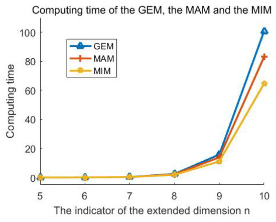
The second simulation was executed to verify the efficiency of the proposed multilevel iteration method. Figure 3a is the original clear ’building’ image with the size $256\times 384$, and the blurred image is recovered in Figure 3b with $\sigma =0.01$ in the blurring kernel and noise level $\delta =0.01$ using the MIM. For comparison, we also conducted experiments using the Gaussian elimination method (GEM) in [28] and the multilevel augmentation method (MAM) in [10]. $T_{GEM}$, $T_{MAM}$ and $T_{MIM}$ represent the computing time of the Gaussian elimination method, the multilevel augmentation method and the multilevel iteration method, respectively. The value n listed in Table 2 ranges from 5 to 10, and in this case, the continuous intensity function (69) is needed. As shown in Section 2, two one-dimensional integral equations are solved to recover the blurred image. Therefore, the computing time here denotes the summation of the time needed to solve the coupled Equation (8) twice. In our MIM experiments, all processes stopped at the second iteration, which is very fast because of the good selection of the initial values ${\tilde{x}}_{\alpha ,k}^{{}^{\delta }}$ and ${\tilde{v}}_{\alpha ,k}^{{}^{\delta }}$. These two initial values can be found in Step 1 of Algorithm 1. Figure 3c–e show the reconstructed images of (b) using the GEM, the MAM and the MIM. Meanwhile, Table 2 and Figure 4 exhibit the computing time of these three methods. On the whole, the computing time of the MIM is the least among the results of these methods. All results show the proposed multilevel iteration method requires less computational resources. The difference is obvious, especially when the indicator of the extended dimension n is large.

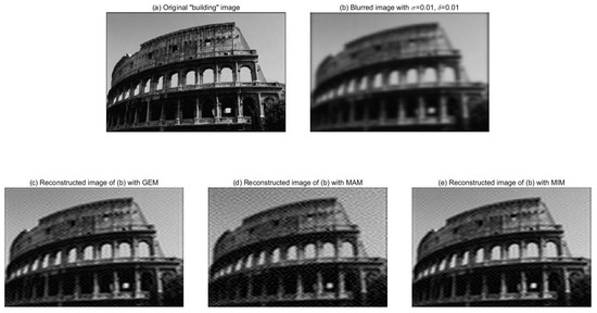
Figure 3. (a) The original clear ’building’ image. (b) Blurred image with $\sigma =0.01$ and $\delta =0.01$. (c–e) are reconstructed images of (b) with the GEM, the MAM, and the MIM.

Table 2. The computing time of the GEM, the MAM and the MIM.

n	5	6	7	8	9	10
$T_{GEM}$	0.0131	0.0645	0.3535	2.4250	15.8140	100.6399
$T_{MAM}$	0.0103	0.0528	0.3454	2.2584	13.8898	82.9874
$T_{MIM}$	0.0084	0.0500	0.3478	1.8875	11.0880	64.6845

Figure 4. The computing time of the GEM, the MAM and the MIM.

Example 3.

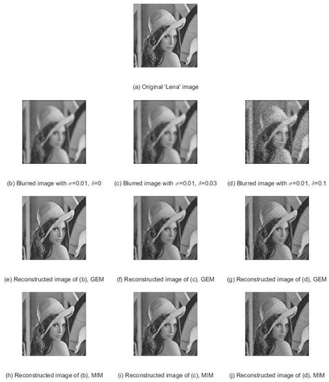
In this example, we demonstrate that the performance of the MIM is as good as the alternative method. As shown in Figure 5b–d, we consider the restoration of the ’Lena’ image, which has the size $257\times 257$. We use the image with $\sigma =0.01$ in the blurring kernel and different noise level δ. Note that when $\delta =0$, the image is noise free. We introduce the peak signal-to-noise ratio (PSNR) to evaluate the restored images and blurred images. For comparison, we solved the corresponding integral equation by using the proposed multilevel iteration method and the Gaussian elimination method with the piecewise linear polynomial basis functions at $n=8$. Table 3 and Table 4 list ${\alpha }_{+}$ obtained from the parameter choice using Rule 1, the PSNR value of the blurred image (PB), the PSNR value of the reconstructed image (PR), and the corresponding time to solve the equation using the GEM and the MIM separately, where the noise level δ ranges from 0 to 0.15. Figure 5e–j show the reconstructed image corresponding to different methods and different noise levels of 0, 0.03, and 0.1. In general, by comparing the numerical experiments in Table 3 and Table 4, we can conclude that there is almost no difference in the PSNR value of the reconstructed image using the GEM and the MIM, but more specifically, the MIM performs better in most cases. But more seriously, the MIM performs better in most cases.

Figure 5. (a) Original clear ’Lena’ image. (b–d) are blurred images with $\sigma =0.01$ in kernel and noise level $\delta =0,0.03,0.1$, respectively. (e–g) are reconstructed images of (b–d) respectively using the GEM. (h–j) are reconstructed images of (b–d) respectively using the MIM.

Table 3. Performance of the Gaussian elimination method.

$\mathit{\delta }$	0	0.01	0.03	0.05	0.10	0.15
${\alpha }_{+}$	4.3980 × ${10}^{-7}$	0.0067	0.0167	0.0256	0.04	0.05
$PB$	23.0173	22.9552	22.4792	21.6726	19.1102	16.7175
$PR$	31.9072	25.8306	24.5039	23.6348	21.9135	20.7536

Table 4. Performance of the multilevel iteration method.

$\mathit{\delta }$	0	0.01	0.03	0.05	0.10	0.15
${\alpha }_{+}$	6.6570 × ${10}^{-6}$	0.009	0.0199	0.0240	0.0394	0.0526
$PB$	23.0173	22.9528	22.4801	21.6692	19.1201	16.7044
$PR$	30.9030	25.9479	24.5537	23.6281	21.9105	20.7557

Example 2, combined with Example 3, proves that the MIM uses less computation time than the alternative methods, while the performance is equally well. Therefore, we can conclude that the multilevel iteration method is an effective fast algorithm to solve the integral equation in image restoration.

7. Conclusions

In this paper, we formulate the problem of image restoration as an integral equation. In order to solve this integral equation, we propose two fast algorithms. The first one is the fully discrete multiscale collocation method, which converts the calculation of the integral to a matrix operation. The second one is the multilevel iteration method, which guarantees that the solution has an optimal order. All examples verify that the proposed methods are accurate and efficient when compared with alternative strategies. In the future, we will still focus on finding faster and more efficient methods.

References

- Lu, Y.; Shen, L.; Xu, Y. Integral equation models for image restoration: High accuracy methods and fast algorithms. Inverse Probl. 2010, 26, 045006. [Google Scholar] [CrossRef]
- Chan, R.H.; Chan, T.F.; Shen, L.; Shen, Z. Wavelet algorithms for high-resolution image reconstruction. SIAM J. Sci. Comput. 2003, 24, 1408–1432. [Google Scholar] [CrossRef]
- Jiang, Y.; Li, S.; Xu, Y. A Higher-Order Polynomial Method for SPECT Reconstruction. IEEE Trans. Med. Imaging 2019, 38, 1271–1283. [Google Scholar] [CrossRef] [PubMed]
- Liu, Y.; Shen, L.; Xu, Y.; Yang, H. A collocation method solving integral equation models for image restoration. J. Integral Eq. Appl. 2016, 28, 263–307. [Google Scholar] [CrossRef]
- Groetsch, C.W. The Theory of Tikhonov Regularization for Fredholm Equations of the First Kind; Research Notes in Mathematics; Pitman (Advanced Publishing Program): Boston, MA, USA, 1984. [Google Scholar]
- Engl, H.W.; Hanke, M.; Neubauer, A. Regularization of Inverse Problems; Mathematics and Its Applications; Kluwer Academic Publishers Group: Dordrecht, The Netherlands, 1996. [Google Scholar]
- Chen, Z.; Ding, S.; Xu, Y.; Yang, H. Multiscale collocation methods for ill-posed integral equations via a coupled system. Inverse Probl. 2012, 28, 025006. [Google Scholar] [CrossRef]
- Russell, R.D.; Shampine, L.F. A collocation method for boundary value problems. Numer. Math. 1972, 19, 1–28. [Google Scholar] [CrossRef]
- Krasnosel’skii, M.A.; Vainikko, G.M.; Zabreiko, P.P.; Rutitskii, Y.B.; Stetsenko, V.Y. Approximate Solution of Operator Equations; Wolters-Noordhoff Pub: Groningen, The Netherlands, 1972. [Google Scholar]
- Chen, Z.; Micchelli, C.A.; Xu, Y. Multiscale Methods for Fredholm Integral Equations; Cambridge Monographs on Applied and Computational Mathematics; Cambridge University Press: Cambridge, UK, 2015. [Google Scholar]
- Micchelli, C.A.; Xu, Y.; Zhao, Y. Wavelet Galerkin methods for second-kind integral equations. J. Comput. Appl. Math. 1997, 86, 251–270. [Google Scholar] [CrossRef]
- Groetsch, C.W. Convergence analysis of a regularized degenerate kernel method for Fredholm integral equations of the first kind. Integral Eq. Oper. Theory 1990, 13, 67–75. [Google Scholar] [CrossRef]
- Hämarik, U.; Raus, T. About the balancing principle for choice of the regularization parameter. Numer. Funct. Anal. Optim. 2009, 30, 951–970. [Google Scholar] [CrossRef]
- Pereverzev, S.; Schock, E. On the adaptive selection of the parameter in regularization of ill-posed problems. SIAM J. Numer. Anal. 2005, 43, 2060–2076. [Google Scholar] [CrossRef]
- Bauer, F.; Kindermann, S. The quasi-optimality criterion for classical inverse problems. Inverse Probl. 2008, 24, 035002. [Google Scholar] [CrossRef]
- Jin, Q.; Wang, W. Analysis of the iteratively regularized Gauss-Newton method under a heuristic rule. Inverse Probl. 2018, 34, 035001. [Google Scholar] [CrossRef]
- Rajan, M.P. Convergence analysis of a regularized approximation for solving Fredholm integral equations of the first kind. J. Math. Anal. Appl. 2003, 279, 522–530. [Google Scholar] [CrossRef][Green Version]
- Ma, Y.; Xu, Y. Computing integrals involved the Gaussian function with a small standard deviation. J. Sci. Comput. 2019, 78, 1744–1767. [Google Scholar] [CrossRef]
- Luo, X.; Fan, L.; Wu, Y.; Li, F. Fast multi-level iteration methods with compression technique for solving ill-posed integral equations. J. Comput. Appl. Math. 2014, 256, 131–151. [Google Scholar] [CrossRef]
- Gonzalez, R.C.; Wintz, P. Digital Image Processing; Addison-Wesley Publishing Co.: Reading, MA, USA; London, UK; Amsterdam, The Netherlands, 1977. [Google Scholar]
- Chen, Z.; Micchelli, C.A.; Xu, Y. A construction of interpolating wavelets on invariant sets. Math. Comp. 1999, 68, 1569–1587. [Google Scholar] [CrossRef]
- Chen, Z.; Xu, Y.; Yang, H. Fast collocation methods for solving ill-posed integral equations of the first kind. Inverse Probl. 2008, 24, 065007. [Google Scholar] [CrossRef]
- Chen, Z.; Xu, Y.; Yang, H. A multilevel augmentation method for solving ill-posed operator equations. Inverse Probl. 2006, 22, 155–174. [Google Scholar] [CrossRef]
- Chen, Z.; Micchelli, C.A.; Xu, Y. Fast collocation methods for second kind integral equations. SIAM J. Numer. Anal. 2002, 40, 344–375. [Google Scholar] [CrossRef]
- Micchelli, C.A.; Xu, Y. Reconstruction and decomposition algorithms for biorthogonal multiwavelets. Multidimens. Syst. Signal Process. 1997, 8, 31–69. [Google Scholar] [CrossRef]
- Fang, W.; Lu, M. A fast collocation method for an inverse boundary value problem. Int. J. Numer. Methods Eng. 2004, 59, 1563–1585. [Google Scholar] [CrossRef]
- Groetsch, C.W. Uniform convergence of regularization methods for Fredholm equations of the first kind. J. Aust. Math. Soc. Ser. A 1985, 39, 282–286. [Google Scholar] [CrossRef][Green Version]
- Kincaid, D.; Cheney, W. Numerical Analysis: Mathematics of Scientific Computing; Brooks/Cole Publishing Co.: Pacific Grove, CA, USA, 1991. [Google Scholar]
- Taylor, A.E.; Lay, D.C. Introduction to Functional Analysis, 2nd ed.; Robert, E., Ed.; Krieger Publishing Co., Inc.: Melbourne, FL, USA, 1986. [Google Scholar]
© 2020 by the authors. Licensee MDPI, Basel, Switzerland. This article is an open access article distributed under the terms and conditions of the Creative Commons Attribution (CC BY) license (http://creativecommons.org/licenses/by/4.0/).