Abstract
Ground level concentrations of nitrogen oxide (NOx) can act as an indicator of air quality in the urban environment. In cities with relatively good air quality, and where NOx concentrations rarely exceed legal limits, adverse health effects on the population may still occur. Therefore, detecting small deviations in air quality and deriving methods of controlling air pollution are challenging. This study presents different data analytical methods which can be used to monitor and effectively evaluate policies or measures to reduce nitrogen oxide (NOx) emissions through the detection of pollution episodes and the removal of outliers. This method helps to identify the sources of pollution more effectively, and enhances the value of monitoring data and exceedances of limit values. It will detect outliers, changes and trend deviations in NO2 concentrations at ground level, and consists of four main steps: classical statistical description techniques, statistical process control techniques, functional analysis and a functional control process. To demonstrate the effectiveness of the outlier detection methodology proposed, it was applied to a complete one-year NO2 dataset for a sub-urban site in Dublin, Ireland in 2013. The findings demonstrate how the functional data approach improves the classical techniques for detecting outliers, and in addition, how this new methodology can facilitate a more thorough approach to defining effect air pollution control measures.
1. Introduction
Nowadays, most cities have an increasing environmental problem related to air pollution [1,2,3,4]. This specific pollution is a continuing threat to human health and welfare, with a range of different sources generating different pollutants which have distinct health effects on urban populations [5,6,7]. Detailed air quality monitoring data for pollutants, such as carbon monoxide (CO), nitrogen oxides (NO and NO2), sulphur dioxide (SO2), ozone (O3) and particulate matter (PM10 and PM2.5), are becoming more important because of the health problems said pollutants can cause in living beings [6]. The measurements of pollutants provide real-time data to inform the public and provide a mechanism of alerting local residents of a possible hazard. In particular, pollutant sources from traffic emissions, such as NOx, which represents a combination of nitrogen oxide (NO) and nitrogen dioxide (NO2), are typically emitted at ground level from vehicles and are associated with health-related problems [8]. Despite a reduction in emissions from the transport sector, an increasing trend in NO2 concentrations has been observed in a number of different European countries; for example, the United Kingdom and Ireland [9,10]. Therefore, meeting the standards and air quality guidelines by European and national environmental agencies for pollutants such as NO2 is becoming more challenging [9], as exceedances of pollutant concentrations can lead to short-term, chronic human health problems [11].
On the other hand, it is understandable that occasional values in polluted air samples behave as outliers in an urban environmental database. They can be classified as local outliers [12,13] or global outliers. Unlike global outliers, local outliers can be detected by comparison with near neighbours. For the purpose of air pollution studies in urban areas, global outliers that deviate from the guide values indicate that there may be a significant source of pollution. Observations which are not excessively high but are different from neighbouring values may also contain information on unusual processes such as pollution. Outliers may merely be noisy observations, or alternatively, they may indicate atypical behaviour in the system. These abnormal values are very important and may lead to useful information or significant discoveries, but also contribute to the selection of the most suitable mitigation techniques or measures [14].
Different techniques of functional data analysis (FDA) have been used in vectorial problems. This new methodology appeared due to the inefficiency of the classical data mining techniques treating vector data [15]. FDA is applicable in a multitude of fields, such as environmental [16,17,18,19] and medical research [20], and is applicable for sensors [21,22] and industrial methods [23,24]. The functional model is based on two ideas that make it unique: it takes into account the time correlation structure of the data and leads to a global view of the problem through curves analysis instead individual observations. This analysis is focused on the comparison of the curves using the functional depths, a variable that measures the centrality of a given curve within a set of curves [25]. Functional depth has already been used in several environmental problems [26,27].
The aspiration of this research is to create a model to detect air pollution episodes and identify outliers in gaseous emissions, and to validate this method using real world data from a suburban air quality monitoring site in Dublin, Ireland. Although many methods are known to identify outliers (from the classical Grubbs test [28] to a test proposed in 2019 by [29]), they are all based on the vector approach. This study was carried out, on one hand, with conventional methods, and on the other hand, with a functional approach; a comparative study between the two methodologies is presented. Each method will be presented and the findings will outline the most effective method for detecting outliers in air pollution monitoring data to enhance its capacity for informing new measures to improve local air quality.
2. Methods
2.1. Case Study—A Sub-Urban Air Quality Monitoring Station in Dublin, Ireland
Ireland has a range of air quality monitoring stations across the country, which are part of the national ambient air quality monitoring programme (AAMP). The data collated from these monitoring sites are used to inform on air quality at the local and national levels, and are being used for forecast modelling. The Blanchardstown sub-urban site is one of the 17 national sites, managed by the Environmental Protection Agency (EPA), which monitors NO2 and is classified as a suburban monitoring site. It is located to the west of Dublin city centre in Ireland [30]. The Blanchardstown air quality monitoring station was selected, as it provided continuous, high-resolution NO2 data emissions over a 1-year period. Its location is adjacent to the major arterial carriageway around Dublin city centre, and as a monitoring location, is therefore affected by traffic emissions. In this manner, NO2 hourly data was collected throughout 2013, with 96% of data capture and availability from [31], and the information needed about weather conditions in Dublin in 2013 was obtained on [32].
EU legislation for NO2 limit values (2008 CAFE Directive and S.I. number 180 of 2011) align with the World Health Organisation (WHO) guidelines, with 1-hour and 1-year limit values of 200 g/m and 40 g/m respectively. In circumstances in which the hourly value is exceeded on three consecutive hours, short-term action plans must be implemented by local authorities to mitigate against continued pollution events (limiting traffic flows, restricting construction work, industrial processes, etc.). Despite there being no daily NO2 limit value in the EU and WHO, some countries have set an average daily limit of 100 g/m (range from 80–150 g/m) [31].
The sources and trends of NO2 emissions over the last 20 years has seen a recent increasing trend due to growth in the transport sector and a recovery since the 2008 economic downturn. As such, Ireland’s air quality in relation to NO2 is considered to be deteriorating, as measurement data suggests it may reach limit values and the national emissions ceiling in the coming years.
2.2. Analysis Methods
A range of systems are available to analyse environmental data, such as air quality measurements. These systems can be used to detect uncharacteristic data points by taking into account trends, variations between neighbouring network stations and expected values with respect to the sampling location. An example of these expert systems of data and environmental parameter validation would be the trends analysis throughout R-programming (openair) [33].
With classical analysis, the data are only analysed statically. The proposed methodology includes using a large amount of existing data to extract conclusions. Today, the amount of data that has been stored in environmental databases requires automated analysis techniques. Actually, the analysis methodology presented here is oriented to knowledge discovery in databses (KDD) [34], which provides a complete process for extracting information and also provides a clear methodology for the preparation of data and interpreting the results obtained. KDD involves an iterative and interactive process of searching for models, patterns and parameters that are useful for detection, classification and/or prediction in order to generate knowledge and help in decision making.
2.2.1. Classical Analysis
The classical monitoring strategy for air quality uses individual time series, descriptive statistics, box plots, autocorrelation analysis, etc., to determine if any of the values fall outside of the limits and to analyse trends [35,36]. In general, classical statistical analysis seeks to describe the distribution of a measurable variable (descriptive statistics) and to determine the consistency of a sample drawn from an initial population (inferential statistics). In addition, classical analysis is based on repetition; one must measure properties of objects and try to predict the frequency of occurrence of results when the measuring operation is repeated at random or stochastically.
This type of analysis determines the empirical frequency distribution that yields the absolute or relative frequency of the occurrence of the different possible results of the repeated measurement of a property of an object (discrete case). Instead, if the case is an infinitely repeated and arbitrarily precise measurement and every outcome is diffferent, the relative frequency of a single outcome would not be very instructive; the distribution function is used, which, for every numerical value x of the measured variable, yields the absolute (or relative) frequency of the occurrence of all values smaller than x [37].
2.2.2. Statistical Process Control
By applying statistical process control (SPC) methods to the monitoring of a system, it is possible to detect outliers. This study is concentrated on significantly high and low measurements, even in situations where the values do not exceed the established limit. These methodologies can be used to study individual observations, using individual or average charts.
The dataset should be partitioned into rational subgroups, minimising the probability of large differences between subgroups [38]. The formation of rational subgroups is important, because variation within subgroups can be clustered and the presence of special causes of variability can be easily detected. However, sometimes it is not practical to use rational subgroups; for example, when repeated measurements in the process differ only by laboratory or analytical error. Even when automated inspection is used, because every unit manufactured is analysed.
The rational subgroups represent the way of collecting the data. Usually, they should be gathered so that each of them shows only the inherent variation that is natural for the process (common cause variation). Because they contribute to identifying any other source of variation (special cause variation) that may badly affect the process, the subgroups should avoid special-cause variation where possible. Moreover, the limits on a control chart, which mark the boundary to identify if a process is too volatile, are calculated on the basis of the variability within each subgroup. For this, only subgroups that reproduce the common cause variation in a process should be selected.
Once the data are correctly structured, a normality test has to be done. If the hypothesis of normality is rejected, there are two possibilities: use modified classical techniques to non-normal distributions [39], or transform the data to normalise the dataset [40]. The second option applies a Box-Cox transformation [41], which smoothes the data structure. The most widely used and known transformation is the Box-Cox transformation, defined as follows:
where maximises the profile likelihood function of the data .
A classical analysis process can be divided in two main stages: the learning stage, when a test of normality is performed and atypical measurements are deleted from the data; and the control stage, when the trends are analysed to encounter out-of-control situations. At the first one, it is when the centreline (CL) and control limits are defined. Specifically, the CL is defined with the control sample and represents the objective value. In addition, the warning limits are set at a distance of from it, and control limits at , with being the standard deviation of the process [42].
Shewhart control charts have been the most widely used due to their good performance in detecting large changes in a process. However, because these charts use the most recent samples, they do not efficiently detect small or progressive changes in a process. In this regard, complementary rules are needed; multiple authors have defined different rules to detect specific deviations [43,44] and to complement the initial control rules [45]. The use of these supplementary rules makes Shewhart’s control charts more sensitive and leads to an improvement in one’s capacity to detect non-random patterns.
A widely used way to quantify the potential of a control chart with supplementary rules is through the average run length (ARL). The ARL, in control charts, is the average number of points that should be analysed before showing an alert warning that the process is not under control. When this occurs, the efficient thing to do would be to detect it as soon as possible. On the contrary, when the process is statistically stable, it would be appropriate to have few false alarms. This term is directly related to a Type I error (also known as ) and a Type II error (also known as ), which also describe the sensitivity of the method, and it is highly related to the number of false alarms. For that reason, it must be contemplated that if the capacity of this methodology to detect out-of-control situations is high, there will be a lot of false alarms [43].
2.2.3. Functional Data Analysis
The functional data analysis works with the observations that come from a continuous random process that is evaluated at discrete points [46]. Starting from vector samples, the dataset will be transformed into a functional sample. The first step is to construct the most appropriate curves from the initial points that come from the discrete values measured in the study. This process, known as smoothing, converts the vector values into continuous functions over time. This structure of data is essential in the air pollution context because it is taking into account all the values in the day as a set. In this way, a day in which NO2 values are obtained with a lot of variability but which has an average similar to the other days, is not detected from any vectorial approach. Functional analysis would identify these types of days as candidates for outliers. Furthermore, in several similar studies in which they also tried to detect outliers with data from certain gases (see [23,47]), the superiority of functional approaches was demonstrated.
In a situation where the initial observations are contained in a set of points, ∈ represents the time steps and is the number of observations . They can be watched as the individual values of the function , F being a functional space. The estimation of takes into account a functional space , where is the set of basis functions and is the number of basis functions required to build a functional sample. There are several types of basis in statistics, but the most used one is the Fourier basis [26,48]. Moreover, with periodic data such as we have in this study, Fourier bases are the most appropriate [49]. Smoothing consists of finding a solution to the regularisation problem [46],
with + being the result of observing x at the point ; the random noise with zero mean, being a penalising operator focused on obtaining the simplest possible solutions; and being a parameter that defines the level of the regularisation. The initial step is the following expansion
where are coefficients that multiply the selected basis functions. The smoothing problem can be written as follows:
with a vector of observations ; a vector of coefficients of the expansion ; a -matrix whose elements are ; and a -matrix R whose elements are:
Finally, the problem is solved [46] according to:
As soon as the data are in functional form, they can be analysed to identify pollution episodes and detect outliers. The functional data allow us to identify whether different periods of time such as days, weeks or months are above the mean function and how much they are deviating. Moreover, it permits the elimination of outliers which are not real; they are due to system fails. The depth concept provides a way for ordering a set of data, contained in a euclidian space, according their proximity to the centre of the sample.
The concept of depth appeared in multivariate analyses, and was created to measure the centrality of a point among a cloud of them [50,51]. Over the years, this concept began to be introduced into functional data analysis [52]. In this field, depth represents the centrality of a certain curve and the mean curve is the centre of the sample. Two depth measurements very common in the context of functional data are: Fraiman-Muniz depth (FMD) [25] and H-modal depth (HMD) [52].
Therefore, the identification of outliers with a functional approach is possible with the calculation of depths. In this case, elements that have different behavioural patterns than the rest will be taken into account. The concept of depth makes it possible to work with observations, defined in a given time interval, in the form of curves, instead of having to summarise the observations of the curve into a single value, such as the mean. This method of outlier detection is based on depth measures and centrality: an element that is far from the centre of the sample will have a low depth. Thus, the curves with the least depth are the functional outliers.
Firstly, the cumulative empirical distribution function of the values of the curves in a certain time it is contemplated. It can be defined as
with being a indicator function. Subsequently, the FMD for any curve within a set of curves is calculated as
where is the depth of the curve , , expressed as
On the other hand, for HMD the functional mode is the element or curve most densely surrounded by the other curves in the dataset. HMD is defined as
with a kernel function , a bandwidth parameter h and as the norm in a functional space. Among all the norms, in the most cases, it is used the norm , expressed as
In addition, also exist several options for the kernel functions . A widely used one is the truncated Gaussian kernel, expressed as
In this paper, the depth chosen to identified outliers is the HMD. The bandwidth h is the value that leaves, below it, 15% of the data coming from the distribution of [15], and the cut-off C is selected, specifically, to have a 1% Type I error [50], according to
The cut-off C has to be estimated because the distribution of the functional depth is not known. There are several ways to carry out this estimation; however, the bootstrapping method is the most appropriate for the purpose of this research [52,53]. The steps to follow are:
- Extract, with replacement, a new sample of the original.
- Estimate the study parameter through the statistic of this new sample.
- Repeat the above steps a large number of times. This repetition is also known as Monte Carlo simulation; it relies on repetition to extract information from the data (see examples in [54,55]).
- Obtain the empirical distribution of the statistic.
2.2.4. Functional Strengths
The functional data analysis (FDA) has many strong points, but the ones that allow the FDA to have a better performance in contamination analysis are the following: [18,19,24]:
- It is not necessary to know anything in advance about the distribution of the data.
- The analysis of the time sets as a unit. The sample analysed is structure in complete time units like days or years. Individually distributed values are not taken into account.
- Analysis of homogeneity. Outliers are defined differently; data which do not exceed the limit but which constantly have small deviations should be classified as outliers.
- Trend analysis. With these techniques, besides detect outliers, also it is possible to analyse situations where there are no outliers but small deviations from the normal data behaviour are observed.
- Complete analysis of the time spectrum. In classic studies, generally, the analyses are based on specific values measured in a determined set of points. The FDA, on the other hand, made it possible to work with the entire time spectrum of a continuous mode.
3. Results and Discussion
The results of the three methodologies presented in this document are presented below. All figures were obtained with the R-programming [56] and Python [57] software.
3.1. Classical Analysis
To perform the classical monitoring strategy on air quality the individual time series, descriptive statistics, box plots and autocorrelation analysis were calculated to determine if any of the values fell outside of the limits, and to analyse trends. The descriptive statistical parameters of the dataset are shown in Table 1:

Table 1.
Summary descriptive statistics of hourly NO2 concentrations from Blanchardstown air quality monitoring station in Dublin, Ireland. The statistical quartiles (Q1, Q2, Q3) and the interquartile range (IQR) are also displayed. Take into account that 0 g/m represents a missing or wrong value.
The descriptive statistical parameters in Table 1 show that the limit values are not exceeded. The next step of classical data analysis is present a time series of the hourly data in 2013 (Figure 1), ranging from the maximum value 153.48 g/m to the minimum value 0 g/m. From here it is possible to say that in any moment, the hourly upper limit (200 g/m) is not exceed and that the data have a high variability.
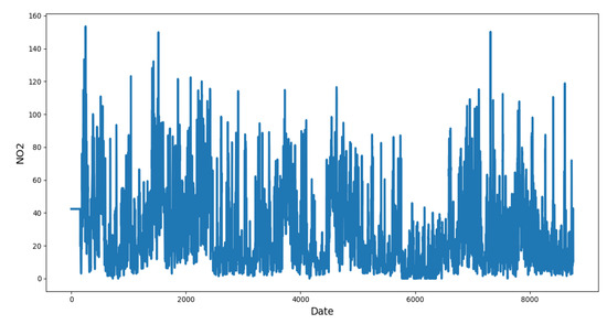
Figure 1.
Individual time series of hourly NO2 concentrations from Blanchardstown air quality monitoring station in Dublin, Ireland. Software: Python [57].
Figure 2 presents a boxplot which graphically characterises the data groups of the NO2 concentration by quartiles. The diagram graphically displays the values of the first quartile (9.56 g/m); third quartile (42.33 g/m); the interquartile range (32.77 g/m); and some, in red, that are considered atypical.
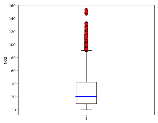
Figure 2.
Box-plot of hourly NO2 concentrations from Blanchardstown air quality monitoring station. The central and blue line represents the median, and the end of the whiskers are the quartiles (25% for the lower part and 75% for the upper part). The red dots represent the outliers. Software: Python [57].
Figure 3 presents the frequency of hourly concentrations of NO2, which, as can be seen, are biased by 0 values. Another weakness of this analysis is that, when data are poorly collected or no data are available, only two options remain: either delete these observations (data are lost) or replace them with 0 values.
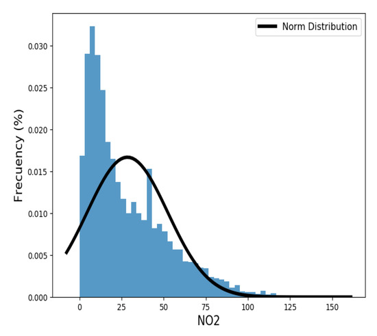
Figure 3.
Frequency of hourly NO2 concentrations from Blanchardstown air quality monitoring station. Comparison of data distribution with normal. Software: Python [57].
Figure 4 shows the normal probability plot of the data, again affected by 0 values. A Kolmogorov-Smirnov test and Anderson Darling test were applied to compare NO2 concentrations to a standard normal distribution [54]. The null hypothesis is that the values have a standard normal distribution. The alternative hypothesis is that the values do not have that distribution. The results obtained for both tests were p-values very close to 0, so, with a 5% significance level, statistical evidence of the non-normality of the data has been found. The test statistic is: , where F(x) is the empirical cumulative distribution function and G(x) is the standard normal cumulative distribution function.
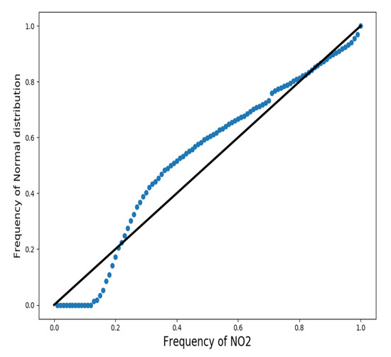
Figure 4.
Normal probability plot of hourly NO2 (QQ-plot) concentrations from Blanchardstown air quality monitoring station. Software: Python [57].
Other tests have been performed to check whether the data approaches any type of distribution: normal, generalised extreme value or Weibull and Rayleigh, but none have been acceptable with a null hypothesis at 5% significance. From the classic analysis of the data it must be concluded that there are no data that are outside the limit values. This classical method is limited to a time series analysis with regard to the assessment of trends (Figure 1), and although it allows for the identification of the main parameters within the data and how the data are distributed, is an incomplete method because it provides us with information that is too simple and does not take into account the correlation between hourly observations.
3.2. Statistical Process Control
3.2.1. Control I-MR Charts with Individual Mean
To analyse the data using the SPC method, an individual-moving range chart (IMR chart) of hourly NO2 concentrations was made. With the examination of the results shown in Figure 5, it can be observed that the number of false alarms, i.e., outliers, is significant. This problem is attributable to:
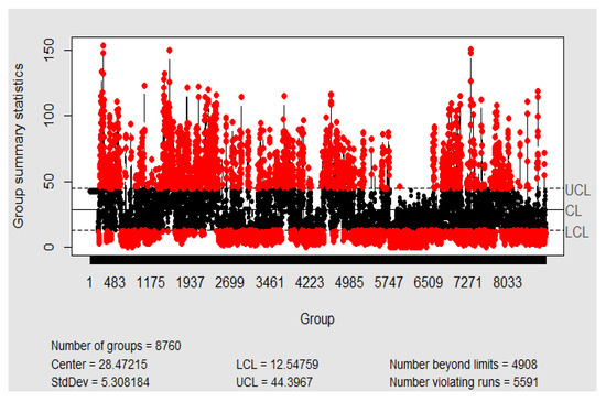
Figure 5.
Individual-moving range chart (IMR chart) X/R with mobile range of hourly NO2 concentrations from Blanchardstown air quality monitoring station. Software: R-programming [56].
- The non-normality of the data, which is clear from the analysis shown in Figure 4.
- The effect of autocorrelation in time series data (Figure 6).
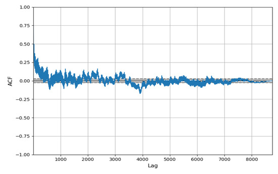 Figure 6. Sample autocorrelation function of hourly values for NO2 concentrations from Blanchardstown air quality monitoring station. Software: Python [57].
 - The existence of greater variability with data of different rational subgroups than within the data inside each analised subgroup.
By performing an autocorrelation analysis, it can be observed from Figure 6 that the data are very autocorrelated. This is very common in environmental data and shows that the autocorrelation has 24-hour cycles and decreases with time.
In Figure 6 the correlation of all data for the year is shown, while Figure 7 only shows the data of the first 86 h in order to see in more detail, the 24 h cycles. Due to the non-normality of the data and the data’s autocorrelation, the control chart has a large number of false alarms. Therefore, SPC is not a very suitable method with which to detect outliers for NO2 concentration.
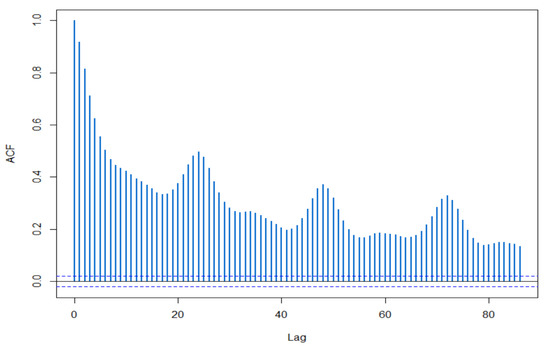
Figure 7.
Sample autocorrelation function of hourly values for NO2 concentrations from Blanchardstown air quality monitoring station over the initial 86 h period. Software: R-programming [56].
3.2.2. Control Charts with Daily Rational Subgroups
The study of datasets choosing days as the rational subgroup of the X/s chart (every day is summed up by one point), is not under control due to the non-normality and the autocorrelation (see Figure 8 and Figure 9). Although the chart is not under control, and there is much variability, none of the 365 days exceed the limit value (100 g/m).
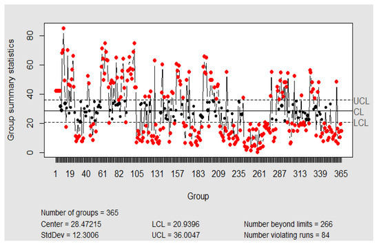
Figure 8.
Xbar-chart of hourly NO2 concentrations with the daily rational subgroup of data. Software: R-programming [56].
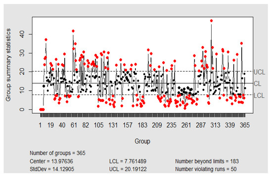
Figure 9.
S-chart of hourly NO2 concentrations with the daily rational subgroup of data. Software: R-programming [56].
3.2.3. Trend Analysis
Using the hourly NO2 concentration data, a trend analysis was undertaken to examine the diurnal patterns and identify outliers. Figure 10 shows the box plots of hourly emissions over 365 days and represents the mean, the confidence interval of this mean, quartiles and abnormal values in red that. This way it is possible to studying individually the distribution of the NO2 emissions in each hour of the day.
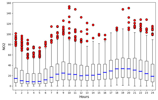
Figure 10.
Hourly box plot of NO2 concentrations from Blanchardstown air quality monitoring station. Software: Python [57].
In Figure 11, where only the mean values have been represented, two maximum values were analysed, at 9 a.m. and 7 p.m., which correspond to heavy traffic hours in this area of Dublin. These two hours, as can be seen in Figure 10, also have high variability (wide boxes), and around them there are numerous outliers.
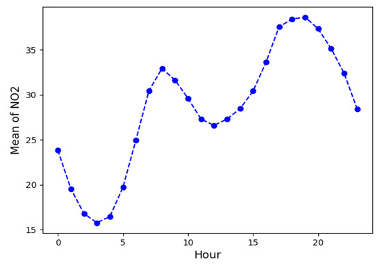
Figure 11.
Mean hourly NO2 concentrations from Blanchardstown air quality monitoring station. Software: Python [57].
It can also be seen in these figures that the absolute minimum is 4 a.m., which also corresponds to the hour with the least variability in the NO2 concentration. If a daily analysis approach is considered throughout the year (Figure 12), it is clear that Wednesday, Thursday and Friday are the days with the highest NO2 concentrations.
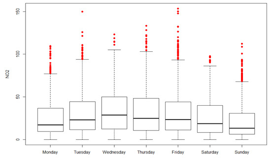
Figure 12.
Daily analysis of NO2 concentrations at Blanchardstown air quality monitoring station. Software: R-programming [56].
Blanchardstown contains the largest shopping centre in Ireland and the most major motorway nearby; because of this, there is a lot of traffic when rush hour and evening shopping are combined in this area. On the other hand, there are lower concentrations during the weekend, although not as low as expected. This is because the largest shopping centre in the country is very busy at weekends, especially during Christmas period.
In this case, a SPC gives us more information than the previous analysis, such as the differences in the NO2 levels between days or hours. However, it still does not take into account the complete daily behaviour of NO2 emissions from correlated hourly measurements.
3.3. Functional Analysis of NO2 in Dublin
The subsequent step in the functional methodology is to compare the results between the classical analysis and the SPC. In the functional methodology, the first thing to do is to build a sample of curves based on the discrete values measured every hour. Figure 13 shows the 365 functions generated with 24 hourly data. Once the data are transformed into functional data, i.e., daily curves of 24 values, each of them takes into account the correlation between the hourly NO2 values and can be analysed for outliers.
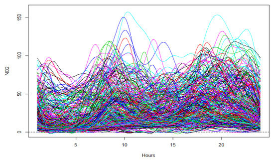
Figure 13.
Data represented in functional form (functions): 365 daily curves of NO2 emissions. Software: R-programming [56].
The results obtained with the functional analysis, taking into account the depths, allow us to identify days with abnormal functional values, even if, discreetly, they are not outliers. Despite not exceeding the daily limit values, the concentration of NO2 over a whole day may have an abnormal behaviour. For this reason the vectorial analysis, like SPC, does not get to detect these days. In a different way, the functional approach detects any deviation from normal daily behaviour in the emissions of NO2, without relying on any distribution restrictions. This is shown in Figure 14 where the functional outliers found in this case study are presented.
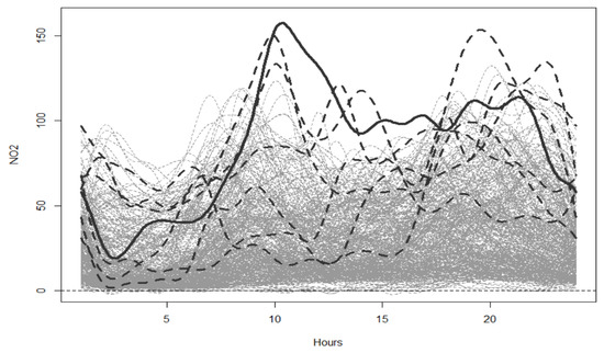
Figure 14.
NO2 functional data; and in the dark grey and dotted line, the functional outliers detected. Highlighted is the 11th day which is also an outlier. Software: R-programming [56].
The data analysed were not discretely outside the limits values; however, functionally excessive variations were observed on specific days. It can be deduced that there were no NO2 pollution problems in 2013 because hourly, daily and annual NO2 concentration limits were not exceeded. But it is also important to analyse whether there are hours or days with anomalous trends of NO2 concentrations, although they remain within legal limits. The NOx (NO, NO2) is an pollutant not coming from a natural source ([58]), and for this reason also, its involvement in the mechanisms of depleting the ozone layer are very unfortunate. The FDA methodology has proven to be very effective in detecting days with trends that are not the same as the rest of the data. It is important not only to analyse whether the contamination is within the allowed limits, but also to find days that are different than expected.
For example, on the 11th day, detected by the functional approach and highlighted in the Figure 14, with the results obtained through the SPC, as can be seen in Figure 8, this day has a higher mean, but it is within the limit values. Neither using the classical analysis (Figure 1) with individual time series nor the one with the corresponding statistical parameters, it could be considered an outlier. Figure 14 shows a strength of the functional approach by detecting this curve as an atypical day; it will be possible to study the reasons that lead the NO2 to behave this way on this particular day. In fact, there are several studies that demonstrate the greater power of the functional approach for detecting outliers than other methodologies (see [17,59]). There are also studies that, specifically, show that the depth measure used here (h-modal) is the one that achieves the lowest error rates [50].
To find a reason that explains the anomalous behaviour on those days, it would be necessary to have greater traceability of the most important sources of NO2 emissions. It would be necessary to have data relating to the weather conditions, traffic movements, industry sources affecting the study area, etc. For example, incorporating weather conditions, i.e., temperatures, sunshine hours and precipitation, could improve the assessment of outliers. The detection of outliers and air pollution episodes can help to separate the causes of normal and specific variability, and is a first step towards the effective design and implementation of mitigation measures. Although the only reason for these outliers is possibly not the weather conditions, as can be seen in Table 2, those days were colder than usual; had very little precipitation; and in general, had fewer sunshine hours than the average for the month.
Table 2.
Sample of other environmental characteristics from Dublin (temperature, sunshine and precipitation) which may impact hourly NO2 concentrations measured at Blanchardstown air quality monitoring station. The averages shown represent the monthly average of each variable.
4. Conclusions
In this paper, three different analytical methods were adopted and compared to determine their effectiveness to identify pollution episodes and outliers. The data used come from a sub-urban air quality monitoring site in Dublin, Ireland, and cover the whole year 2013 with hourly measurements. Firstly, a classical vectorial approach was applied by analysing the data through time series, boxplots and frequency plots. Secondly, a statistical process control was adopted to study the data grouped by days or hours, and with different control charts (Xbar-chart, S-chart). Finally, to identify air pollution episodes and outliers, a functional data analysis approach was adopted to analyse the daily patterns of NO2 concentrations.
To effectively support the mitigation of air pollution and provide true air quality conditions, a new approach and set of tools are required to effectively assess local air pollution. With this in mind, the classical or vectorial approach is too simplistic, despite providing significant information for decision making. It has several weaknesses related to the time correlation structure of the data, and the inability to detect real outliers, days with behaviours far from the standard, just because they do not exceed limit values. As such, more advanced and modern techniques can provide deeper insights to support controlling air pollution episodes. Statistical process control presents similar problems. Even though it manages to take into account the correlation between data, the lack of normality causes a significant increase in false alarms for days that are within the legal limits; this method labels them as outliers. This is because it works with discrete observations and it is not able to extract continuous information from the data.
Alternately, the functional data analysis method, adapted to study pollution episodes, as shown in this paper, presents important improvements as a method that can be extrapolated to any city in the world. In short, it is not restricted to certain characteristics of the data distribution; takes into account complete time units; works with the entire time spectrum of a continuous mode; and the detection of outliers is more effective, which is very important in pollution issues. On the contrary, working from a functional point of view can also have its drawbacks, such as the need for large amounts of data (it is not always possible to get them), or other data constraints, such as continuity, positivity and monotonicity. But as explained, the fact that all the hourly values of a day are not outliers does not mean that that the day is not an outlier. The outlier search with the FDA allows one to detect days that, for some reason, have different sets of measurements of NO2 than the rest (usually higher or with strange peaks). Being able to study the reasons that make these daily functions behave differently from others makes it possible to prevent them; to try to reduce the variability in emissions; and in short, to improve air pollution control. With a classical method there would be no possibility of relating certain events to lost hours that are labelled as outliers.
The FDA’s approach is presented in this document as a methodology for more effective assessment of air pollution, which is hazardous to the health of living beings, and to inform effective mitigation measures in the future.
Author Contributions
The tasks of this paper were divided as follows: on the one hand, J.P.P., J.S.V. and M.M.C. focused on the development of the mathematical methodology; on the other hand, J.M.T., A.M. and J.G. focused on the environmental part of the work. All authors have read and agreed to the published version of the manuscript.
Funding
This paper was funded by the Spanish Government (Industry and Competitiveness Ministry) under the project RTI2018-096296-B-C21.
Acknowledgments
This paper was supported by the Spanish Government (Industry and Competitiveness Ministry) under the project RTI2018-096296-B-C21.
Conflicts of Interest
The authors declare no conflict of interest.
References
- García Nieto, P. Parametric study of selective removal of atmospheric aerosol by coagulation, condensation and gravitational settling. Int. J. Environ. Health Res. 2001, 11, 151–162. [Google Scholar] [CrossRef] [PubMed]
- Akkoyunku, A.; Ertürk, F. Evaluation of air pollution trends in Istanbul. Int. J. Environ. Health Res. 2003, 18, 388–398. [Google Scholar]
- Karaca, F.; Alagha, O.; Ertürk, F. Statistical characterization of atmospheric PM10 and PM2.5 concentrations at a non-impacted suburban site of Istanbul, Turkey. Chemosphere 2005, 59, 183–190. [Google Scholar] [CrossRef] [PubMed]
- García Nieto, P. Study of the evolution of aerosol emissions from coal-fired power plants due to coagulation, condensation, and gravitational settling and health impact. J. Environ. Manag. 2006, 79, 372–382. [Google Scholar] [CrossRef] [PubMed]
- RCPCH. Every Breath We Take: The Lifelong Impact of Air Pollution; Royal College of Physicians: London, UK, 2016; Available online: https://www.rcplondon.ac.uk/projects/outputs/every-breath-we-take-lifelongimpact-air-pollution (accessed on 7 February 2020).
- WHO. Review of Evidence on Health Aspects of Air Pollution—REVIHAAP Project; World Health Organization: Geneva, Switzerland, 2013; Available online: http://www.euro.who.int/__data/assets/pdf_file/0004/193108/REVIHAAP-Final-technical-report.pdf (accessed on 7 February 2020).
- Kumar, P.; Druckman, A.; Gallagher, J.; Gatersleben, B.; Allison, S.; Eisenman, T.S.; Hoang, U.; Hama, S.; Tiwari, A.; Sharma, A.; et al. The nexus between air pollution, green infrastructure and human health. Environ. Int. 2019, 133, 105181. [Google Scholar] [CrossRef] [PubMed]
- EPA. United States Environmental Protection Agency. 2019. Available online: https://www.epa.gov/ (accessed on 19 December 2019).
- AQEG. Trends in Primary Nitrogen Dioxide in the UK; Air Quality Expert Group, 2007. Available online: https://uk-air.defra.gov.uk/assets/documents/reports/aqeg/primary-no-trends.pdf (accessed on 7 February 2020).
- EPA. Ireland’s Transboundary Gas Emissions; Environmental Protection Agency: Washington, DC, USA, 2018. Available online: http://www.epa.ie/pubs/reports/air/airemissions/Irelands%20Air%20Pollutant%20Emissions%202016.pdf (accessed on 7 February 2020).
- Costa, S.; Ferreira, J.; Silveira, C.; Costa, C.; Lopes, D.; Relvas, H.; Borrego, C.; Roebeling, P.; Miranda, A.I.; Teixeira, J.P. Integrating Health on Air Quality Assessment—Review Report on Health Risks of Two Major European Outdoor Air Pollutants: PM and NO2. J. Toxicol. Environ. Heal. Part B 2014, 17, 307–340. [Google Scholar] [CrossRef]
- Cooper, C.; Alley, F. Air Pollut. Control; Waveland Press: New York, NY, USA, 2002. [Google Scholar]
- Lutgens, F.; Tarbuck, E. The Atmosphere: An Introduction to Meteorology; Prentice Hall: New York, NY, USA, 2001. [Google Scholar]
- Jeanjean, A.; Gallagher, J.; Monks, P.; Leigh, R. Ranking current and prospective NO2 pollution mitigation strategies: An environmental and economic modelling investigation in Oxford Street, London. Environ. Pollut. 2017, 225, 587–597. [Google Scholar] [CrossRef]
- Cuevas, A.; Fraiman, R. A plug-in approach to support estimation. Ann. Stat. 1997, 25, 2300–2312. [Google Scholar]
- Matías, J.; Ordóñez, C.; Taboada, J.; Rivas, T. Functional support vector machines and generalized linear models for glacier geomorphology analysis. Int. J. Comput. Math. 2009, 86, 275–285. [Google Scholar]
- Martínez, J.; Garcia Nieto, P.; Alejano, L.; Reyes, A. Detection of outliers in gas emissions from urban areas using functional data analysis. J. Hazard. Mater. 2011, 186, 144–149. [Google Scholar]
- Martínez, J.; Saavedra, A.; García Nieto, P.; Piñeiro, J.; Iglesias, C.; Taboada, J.; Sancho, J.; Pastor, J. Air quality parameters outliers detection using functional data analysis in the Langreo urban area (Northern Spain). Appl. Math. Comput. 2014, 241, 1–10. [Google Scholar]
- Sancho, J.; Iglesias, C.; Piñeiro, J.; Martínez, J.; Pastor, J.; Araújo, M.; Taboada, J. Study of water quality in a spanish river based on statistical process control and functional data analysis. Math. Geosci. 2016, 48, 163–186. [Google Scholar]
- Dombeck, D.; Graziano, M.; Tank, D. Functional clustering of neurons in motor cortex determined by cellular resolution imaging in awake behaving mice. J. Neurosci. 2009, 29, 13751–13760. [Google Scholar]
- Wu, D.; Huang, S.; Xin, J. Dynamic compensation for an infrared thermometer sensor using least-squares support vector regression (LSSVR) based functional link artificial neural networks (FLANN). Meas. Sci. Technol. 2008, 19, 105202.1–105202.6. [Google Scholar]
- Ordoñez, C.; Martínez, J.; Cos Juez, J.; Sánchez Lasheras, F. Comparison of GPS observations made in a forestry setting using functional data analysis. Int. J. Comput. Math. 2011, 89, 402–408. [Google Scholar]
- Ordóñez, C.; Martínez, J.; Saavedra, A.; Mourelle, A. Intercomparison Exercise for Gases Emitted by a Cement Industry in Spain: A Functional Data Approach. J. Air Waste Manag. Assoc. (1995) 2011, 61, 135–141. [Google Scholar] [CrossRef]
- Sancho, J.; Pastor, J.; Martínez, J.; García, M. Evaluation of Harmonic Variability in Electrical Power Systems through Statistical Control of Quality and Functional Data Analysis. Procedia Eng. 2013, 63, 295–302. [Google Scholar] [CrossRef]
- Fraiman, R.; Muniz, R. Trimmed means for functional data. Test 2001, 10, 419–440. [Google Scholar]
- Piñeiro, J.; Martínez, J.; García Nieto, P.; Alonso, J.; Díaz, C.; Taboada, J. Analysis and detection of outliers in water quality parameters from different automated monitoring stations in the Miño river basin (NW Spain). Ecol. Eng. 2013, 60, 60–66. [Google Scholar]
- Sancho, J.; Martínez, J.; Pastor, J.; Taboada, J.; Piñeiro, J.; García Nieto, P. New methodology to determine air quality in urban areas based on runs rules for functional data. Atmos. Environ. 2014, 83, 185–192. [Google Scholar]
- Grubbs, F.E. Procedures for Detecting Outlying Observations in Samples. Technometrics 1969, 11, 1–21. [Google Scholar] [CrossRef]
- Jäntschi, L. A test detecting the outliers for continuous distributions based on the cumulative distribution function of the data being tested. Symmetry 2019, 11, 835. [Google Scholar] [CrossRef]
- EPA. Air Quality in Ireland 2018; Environmental Protection Agency: Washington, DC, USA, 2019. Available online: http://www.epa.ie/pubs/reports/air/quality/Air%20Quality%20In%20Ireland%202018.pdf (accessed on 7 February 2020).
- EPA. Air Quality in Ireland 2013: Key Indicators of Ambient Air Quality; Environmental Protection Agency: Washington, DC, USA, 2014. Available online: https://www.epa.ie/pubs/reports/air/quality/Air%20Quality%20Report%202013.pdf (accessed on 7 February 2020).
- Romer, U. Weather Online(Ireland). 2013. Available online: https://www.weatheronline.co.uk/weather/maps/current?TYP=tmin&KEY=IE&LANG=en&ART=tabelle&JJ=xxxx&SORT=2&INT=24 (accessed on 19 December 2019).
- Carslaw, D.; Ropkins, K. Openair—An R package for air quality data analysis. Environ. Model. Softw. 2012, 27–28, 52–61. [Google Scholar]
- Piatesky-Shapiro, G.; Frawley, W. Knowledge Discovery in Databases; MIT Press: Cambridge, MA, USA, 1991. [Google Scholar]
- Takeuchi, J.; Yamanishi, K. A unifying framework for detecting outliers and change points from time series. IEEE Trans. Knowl. Data Eng. 2006, 18, 482–492. [Google Scholar] [CrossRef]
- Sim, C.; Gan, F.; Chang, T. Outlier Labeling With Boxplot Procedures. J. Am. Stat. Assoc. 2005, 100, 642–652. [Google Scholar] [CrossRef]
- Montgomery, D. Design and Analysis of Experiments; John Wiley & Sons, Inc.: Hoboken, NJ, USA, 2013; Chapter 1–2; pp. 1–65. [Google Scholar]
- Shewhart, W. Economic Control of Quality of Manufactured Product; Van Nostrand Company: New York, NY, USA, 1931. [Google Scholar]
- Chen, Y.K. An evolutionary economic-statistical design for VSIXcontrol charts under non-normality. J. Adv. Manuf. Technol. 2003, 22, 602–610. [Google Scholar]
- Freeman, J.; Modarres, R. Inverse Box-Cox: the power-normal distribution. Stat. Probab. Lett. 2006, 76, 764–772. [Google Scholar]
- Box, G.; Cox, D. An analysis of transformations. J. R. Stat. Soc. Ser. B (Stat. Methodol.) 1964, 26, 211–252. [Google Scholar]
- Grant, E.; Leavenworth, R. Statistical Quality Control; McGraw-Hill: New York, NY, USA, 1998. [Google Scholar]
- Champ, C.; Woodall, W. Exact results for Shewhart control charts with supplementary runs rules. Technometrics 1987, 29, 393–399. [Google Scholar]
- Zhang, M.; Lin, W.; Klein, S.; Bacmeister, J.; Bony, S.; Cederwall, R.; Del Genio, A.; Hack, J.; Loeb, N.; Lohmann, U.; et al. Comparing clouds and their seasonal variations in 10 atmospheric general circulation models with satellite measurements. J. Geophys. Res. 2005, 110. [Google Scholar] [CrossRef]
- Electric, W. Statistical Quality Control Handbook; AT&T Technologics: Indianapolis, Indiana, 1956. [Google Scholar]
- Ramsay, J.; Silverman, B. Functional Data Analysis; Springer: New York, NY, USA, 2005. [Google Scholar]
- Sánchez-Lasheras, F.; Ordóñez, C.; Garcia Nieto, P.J.; García-Gonzalo, E. Detection of outliers in pollutant emissions from the Soto de Ribera coal-fired plant using Functional Data Analysis: A case study in northern Spain. Proceedings 2018, 2, 1473. [Google Scholar] [CrossRef]
- Muñiz, C.D.; García Nieto, P.J.; Alonso Fernández, J.R.; Torres, J.V.; Taboada, J. Detection of outliers in water quality monitoring samples using functional data analysis in San Esteban estuary (Northern Spain). Sci. Total. Environ. 2012, 439, 54–61. [Google Scholar]
- Kamada, M.; Toraich, K.; Mori, R. Periodic spline orthonormal bases. J. Approx. Theory 1988, 55, 27–34. [Google Scholar]
- Febrero, M.; Galeano, P.; González-Manteiga, W. Outlier detection in functional data by depth measures, with application to identify abnormal NOx levels. Environmetrics 2008, 19, 331–345. [Google Scholar]
- Zuo, Y.; Serfling, R. General notions of statistical depth function. Ann. Stat. 2000, 28, 461–482. [Google Scholar]
- Cuevas, A.; Febrero, M.; Fraiman, R. On the use of the bootstrap for estimating functions with functional data. Comput. Stat. Data Anal. 2006, 51, 1063–1074. [Google Scholar]
- Cuevas, A. A partial overview of the theory of statistics with functional data. J. Stat. Plan. Inference 2014, 147, 1–23. [Google Scholar]
- Jäntschi, L.; Bolboacă, S.D. Computation of Probability Associated with Anderson-Darling Statistic. Mathematics 2018, 6, 88. [Google Scholar] [CrossRef]
- Jäntschi, L.; Bolboacă, S.D. Rarefaction on natural compound extracts diversity among genus. J. Comput. Sci. 2014, 5, 363–367. [Google Scholar] [CrossRef]
- R Core Team. R: A Language and Environment for Statistical Computing; R Foundation for Statistical Computing: Vienna, Austria, 2014. [Google Scholar]
- Van Rossum, G.; Drake, F.L., Jr. Python Reference Manual; Centrum voor Wiskunde en Informatica: Amsterdam, The Netherlands, 1995. [Google Scholar]
- Cosma, C.; Suciu, I.; Jäntschi, L.; Bolboaca, S. Ion-Molecule Reactions and Chemical Composition of Emanated from Herculane Spa Geothermal Sources. Int. J. Mol. Sci. 2008, 9, 1024–1033. [Google Scholar] [CrossRef]
- Yu, G.; Zou, C.; Wang, Z. Outlier Detection in Functional Observations With Applications to Profile Monitoring. Technometrics 2012, 54, 308–318. [Google Scholar] [CrossRef]


© 2020 by the authors. Licensee MDPI, Basel, Switzerland. This article is an open access article distributed under the terms and conditions of the Creative Commons Attribution (CC BY) license (http://creativecommons.org/licenses/by/4.0/).