Time-Consistent Investment and Reinsurance Strategies for Mean-Variance Insurers under Stochastic Interest Rate and Stochastic Volatility

Abstract

This paper studies the time-consistent optimal investment and reinsurance problem for mean-variance insurers when considering both stochastic interest rate and stochastic volatility in the financial market. The insurers are allowed to transfer insurance risk by proportional reinsurance or acquiring new business, and the jump-diffusion process models the surplus process. The financial market consists of a risk-free asset, a bond, and a stock modelled by Heston’s stochastic volatility model. Interest rate in the market is modelled by the Vasicek model. By using extended dynamic programming approach, we explicitly derive equilibrium reinsurance-investment strategies and value functions. In addition, we provide and prove a verification theorem and then prove the solution we get satisfies it. Moreover, sensitive analysis is given to show the impact of several model parameters on equilibrium strategy and the efficient frontier.

1. Introduction

Risk management is a fundamental challenge for insurance companies. Reinsurance is a powerful tool for insurers to transfer insurance risk. Accordingly, it is still a fascinating topic among insurers to design optimal reinsurance contract. On the other hand, increasing insurance companies participate in financial markets nowadays. In this context, the reinsurance and investment problem has become a popular research topic in recent years. For example, Browne (1995) [1] considered the problem of maximizing the expected utility and minimizing the ruin probability for insurers. They derived the optimal investment strategies in a simple setting, where the surplus process is modelled by a drifted Brownian motion. Yang and Zhang (2005) [2] solved this problem in a jump-diffusion surplus process case. Schmidli (2002) [3] considered the problem of minimizing the ruin probability by investment and proportional reinsurance. Bai and Guo (2008) [4] investigated the problem of optimal proportional reinsurance and investment with multiple risky assets under no-short selling constraints. Li et al. (2018) [5] discussed the problem of maximizing expected utility in the case of excess-of-loss reinsurance under model uncertainty. We refer the readers to Guan and Liang (2014) [6] and Zhang et al. (2016) [7] for the criterion of maximizing the utility of terminal wealth, and Liang (2018) [8] for minimizing the ruin probability.

Besides these two criterions, the mean-variance has also been a popular criterion in asset allocation problems since the breakthrough of Markowitz (1952) [9]. Zhou and Li (2000) [10] analytically solved the continuous-time mean-variance problems by stochastic linear-quadratic control theory. In recent years, there has been growing interest in the reinsurance-investment problem under a mean–variance framework, see, for example, Bäuerle (2005) [11], Bai and Zhang (2008) [12], Bi and Guo (2013) [13], and Shen et al. (2014) [14]. In fact, these papers searched pre-commitment solution, which is not time-consistent in the sense that an optimal strategy that is derived at one time is not guaranteed to be optimal at a future time point. Because time-consistency is a basic requirement for decision makers, much literature has recently searched time-consistent mean-variance portfolio selection problems in the Nash equilibrium decision framework that was introduced by Björk et al. (2014) [15] and Björk et al. (2017) [16]. Among them, Zeng and Li (2011) [17] conducted the first study of the time-consistent mean-variance reinsurance-investment problem. They got closed form solutions with the Black-Scholes model by means of extended HJB equations. Subsequently, many related work appears, for example, Zeng and Li (2013) [18] incorporated jumps into this problem, Zhao et al. (2016) [19] considered this problem when assuming that there is a defaultable asset. Xiao et al. (2019) [20] considered the problem of maximizing joint interests of the insurer and the reinsurer. Zhu et al. (2019) [21] considered non-zero sum differential reinsurance and investment game between mean-variance insurers.

A lot of empirical evidence show that the volatilities of risky assets prices are not constant or deterministic; Heston et al. (1993) [22] introduced a stochastic volatility model, which is still popular for option pricing or asset pricing. Additionally, several papers also used this model or its extension in portfolio selection problems, for example, Li et al. (2012) [23], Liu (2007) [24], and Yan et al. (2020) [25]. Additionally, it is generally accepted that the interest rate is stochastic, and popular models describing interest rate include the CIR model and Vasicek model. It is natural to consider their combination, for example, Heston-CIR model or Heston-Vasicek model. In fact, several papers considered hybrid stochastic interest rate and stochastic volatility model in the literature, for example, Ahlip et al. (2013) [26] used this model in foreign option pricing and Guan and Liang (2014) [27] in asset allocation for DC pension plan. However, up to our knowledge, few papers discussed the reinsurance and investment problem in stochastic interest rate enviroment. Although Guan and Liang (2014) [6] and Li et al. (2015) [28] studied the management of interest risk for an insurer, the real interest rate in their work is deterministic. Accrdingly, in the real market, there, in fact, does not exist interest rate risk. Additionally, as the wealth process does not satisfy the usual Lipschitz conditions in stochastic interest rate model, we cannot use standard verification theorem directly when incorporating stochastic rate into the portfolio selection problem. Korn et al. (2002) [29] considered the portfolio selection problem with a stochastic interest rate for CRRA investors and provided a verification theorem. Pan et al. (2017) [30] studied the asset-liability management problem in stochastic interest rate environment for CARA investor. In this paper, we consider the reinsurance-investment problem under the dynamic mean-variance framework. We give a verification theorem for time-consistent mean-variance insurers based on the result of Björk et al. (2017) [16] and verify that the solution we obtain satisfies it.

In our paper, we consider the time-consistent reinsurance and investment problem for mean-variance insurer incorporating both stochastic interest rate and stochastic volatility risk. We use the Heston model to describe the dynamics of stock and the Vasicek model to describe interest rate. The surplus process is modelled by the jump-diffusion process. The insurer can transfer part of risk by proportional reinsurance. The zero coupon bond is included in the financial market in order to hedge interest risk. The objective of insurer is to find an optimal reinsurance investment strategy in a time consistent sense, so as to maximize the expected value of terminal wealth and minimize the associated variance. The contribution of our paper is threefold: (1) we consider the time-consistent mean-variance optimization problem for insurers when considering both stochastic interest rate and stochastic volatility, which is new in the literature. (2) We derive the time consistent equilibrium investment and reinsurance strategies and the value functions explicitly overcoming the difficulties caused by stochastic interest rate. (3) We verify our solution through a verification theorem. It can be seen as an extension of Björk et al. (2017) [16] to stochastic interest rate case and is also new in the literature as we know.

The remainder of this paper is organized, as follows. Section 2 describes model and assumptions. Section 3 formulates the problem in a game theoretic framework and provides the verification theorem. Section 4 derives the equilibrium reinsurance-investment strategy and efficient frontier through an extended HJB equation. Section 5 gives several numerical examples to show the effects of different model parameters on equilibrium strategies and the efficient frontier. We conclude this paper in Section 6.

2. Model Setup

Let $(\mathsf{\Omega },\mathcal{F},\mathbb{P})$ be a complete probability space with a right continuous filtration $\mathcal{F}:={\left\{{\mathcal{F}}_t\right\}}_{t\in [0,T]}$ satisfying usual conditions, where $T\in (0,+\infty )$ represents the time horizon. We assume that all of the stochastic processes in this paper are well defined and adapted to ${\mathcal{F}}_t$.

2.1. The Financial Market

In our model, we assume that the insurer can continuously invest in three assets: risk-free asset, bond, and stock. The dynamics of instantaneous interest rate follows Vasicek model:

$$\mathrm{d}r\left(t\right)=(a-br\left(t\right))\mathrm{d}t-{\sigma }_r\mathrm{d}{W}_r\left(t\right),r\left(0\right)=r_0,$$

(1)

where $a,b$ and ${\sigma }_r$ are positive constants and $W_r\left(t\right)$ is a standard Brownian motion on the probability space.

The price process of risk-free asset $S_0\left(t\right)$ follows:

$$\begin{array}{c}\hfill \frac{\mathrm{d}{S}_0\left(t\right)}{S_0\left(t\right)}=r\left(t\right)\mathrm{d}t,S_0\left(0\right)=s_0.\end{array}$$

The second asset is zero-coupon bond. It is an asset that delivers a payment of $\$1$ at maturity. Denote the price of zero-coupon with maturity s at time t with interest rate $r\left(t\right)=r$ as $B(t,s,r)$. We define the risk-neutral probability measure $\mathbb{Q}$ by $\frac{\mathrm{d}\mathbb{Q}}{\mathrm{d}\mathbb{P}}{|}_{{\mathcal{F}}_T}=G\left(T\right)$, where:

$$G\left(t\right)=exp\{{\int }_0^T{\lambda }_r\left(s\right)\mathrm{d}{W}_r\left(s\right)-\frac{1}{2}{\int }_0^T{\lambda }_r{\left(s\right)}^2\mathrm{d}s\}.$$

Here, ${\lambda }_r\left(s\right)$ is the market risk price of $W_r\left(t\right)$. We assume it to be a constant in this paper. Under $\mathbb{Q}$, we have:

$$B(t,s,r)=E_{\mathbb{Q}}[exp(-{\int }_t^{s}r\left(u\right)\mathrm{d}u)|r\left(t\right)=r].$$

By the Feynman-Kac Theorem, for a fixed s, B satisfies the following PDE:

$$\left\{\begin{array}{cc}\hfill B_t+B_r(a-br+{\lambda }_r{\sigma }_r)+\frac{1}{2}{\sigma }_r^2{B}_{rr}-rB& =0,\hfill \\ \hfill B(s,s,r)& =1,\hfill \end{array}\right.$$

(2)

the bond price is known in an explicit form:

$$B(t,s,r)=exp(-h(s-t)r+\overline{h}(s-t)),$$

(3)

where

$$h\left(t\right)=\frac{1-e^{-bt}}{b},$$

and

$$\overline{h}\left(t\right)={\int }_0^t[\frac{1}{2}{\sigma }_r^{2}h{\left(s\right)}^2-(a+{\lambda }_r{\sigma }_r)h\left(s\right)\mathrm{d}s].$$

From now on we use a shorter notation $B(t,s)=B(t,s,r)$. Applying Itô’s formula, we can obtain $\mathbb{P}$-dynamics of bond:

$$\left\{\begin{array}{cc}\hfill \frac{\mathrm{d}B(t,s)}{B(t,s)}& =r\left(t\right)\mathrm{d}t+h(s-t){\sigma }_r\times ({\lambda }_r\mathrm{d}t+\mathrm{d}{W}_r\left(t\right)),\hfill \\ \hfill B(s,s)& =1.\hfill \end{array}\right.$$

(4)

It is unrealistic to assume that we can find all of the zero-coupon bonds in the market. Following Guan and Liang (2014) [27], we introduce a rolling bond with constant maturity K in our analysis. Denote the price of rolling bond at time t as $B_K\left(t\right)$; $B_K\left(t\right)$ follows the following stochastic differential equation:

$$\frac{\mathrm{d}{B}_K\left(t\right)}{B_K\left(t\right)}=r\left(t\right)\mathrm{d}t+h\left(K\right){\sigma }_r({\lambda }_r\mathrm{d}t+\mathrm{d}{W}_r\left(t\right)).$$

(5)

Because the rolling bond is only correlated with the interest rate and the interest rate model is a one-factor model here, it can be used in order to replicate any zero coupon bond. The relation between rolling bond and zero-coupon bond satisfies:

$$\frac{\mathrm{d}B(t,s)}{B(t,s)}=(1-\frac{h(s-t)}{h\left(K\right)})\frac{\mathrm{d}{S}_0\left(t\right)}{S_0\left(t\right)}+\frac{h(s-t)}{h\left(K\right)}\frac{\mathrm{d}{B}_K\left(t\right)}{B_K\left(t\right)}.$$

The third asset is stock, whose dynamics evolves according to the Heston stochastic volatility model:

$$\left\{\begin{array}{cc}\hfill \frac{\mathrm{d}{S}_1\left(t\right)}{S_1\left(t\right)}& =r\left(t\right)\mathrm{d}t+{\sigma }_S{\sigma }_r\times ({\lambda }_r\mathrm{d}t+\mathrm{d}{W}_r\left(t\right))\hfill \\ \hfill & +\nu L\left(t\right)\mathrm{d}t+\sqrt{L\left(t\right)}\mathrm{d}{W}_S\left(t\right),S_1\left(0\right)=s_1>0,\hfill \\ \hfill \mathrm{d}L\left(t\right)& =\kappa (\delta -L(t\left)\right)\mathrm{d}t+{\sigma }_L\sqrt{L\left(t\right)}\mathrm{d}{W}_L\left(t\right),L\left(0\right)=l_0>0,\hfill \end{array}\right.$$

(6)

where ${\sigma }_S$, ${\sigma }_L$, $\kappa$, $\nu$, $\delta$ are positive constants, $W_S\left(t\right)$ and $W_L\left(t\right)$ are two correlated one-dimensional Brownian motion independent of $W_r\left(t\right)$ in the interest rate model, and $Cov(W_S\left(t\right),W_L\left(t\right))=\rho t$. The condition $2\kappa \delta >{\sigma }_L^2$ is required here in order to ensure $L\left(t\right)>0$.

2.2. Surplus Process

We assume that the insurer’s surplus process is modelled by the following jump-diffusion process:

$$\mathrm{d}R\left(t\right)=c\mathrm{d}t+{\sigma }_0\mathrm{d}{W}_0\left(t\right)-\mathrm{d}\sum _{i=1}^{N\left(t\right)}{Y}_i,$$

where $c>0$ is the premium rate and ${\sigma }_0$ is a positive constant. $W_0\left(t\right)$ is a standard Brownian motion and ${\sigma }_0{W}_0\left(t\right)$ can be seen as the uncertainty from the premium of insurer. $N\left(t\right)$ represents the number of claims between $[0,t]$, which is a Poisson process with intensity $\lambda >0$. $Y_i$ is the size of the ith claim and $Y_i,i=1,2,\dots$ are independent and identically distributed positive random variables with distribution function $F_Y$. Here, $W_0\left(t\right)$ and ${\sum }_{i=1}^{N\left(t\right)}{Y}_i$ are independent with each other and both are independent with $W_S\left(t\right)$, $W_r\left(t\right)$, and $W_L\left(t\right)$. We assume that the moment generating function of $Y_i$ exists, which implies that momentum of each order exists. We denote the first-order moment of the random variable by ${\mu }_y=E\left[Y_i\right]$ and the second-order moment by ${\sigma }_y^2=E\left[Y_i^2\right]$. The insurer calculates the premium rate by the expected value principle, which is, $c=(1+\theta )\lambda {\mu }_y$, where $\theta$ is the safety loading of insurer.

Suppose that the insurer can control risk by proportional reinsurance. We denote $\alpha \left(t\right)$ as the reinsurance proportion of insurer at time t, i.e., the insurer pays $100\alpha \left(t\right)\%$ of the claim while the reinsurer pays $100(1-\alpha (t\left)\right)\%$. Accordingly, $\alpha \left(t\right)$ can also be seen as insurance risk exposure of insurer. If $\alpha \left(t\right)\in [0,1]$, the insurer purchases reinsurance from the reinsurer, if $\alpha \left(t\right)>1$, the insurer acquires new business from the reinsurer, i.e., the insurer acts as a reinsurer of the reinsurer. The reinsurer also uses the expected value principle in order to calculate the premium rate. The insurer has to pay a premium at the rate of $(1+\eta )\lambda {\mu }_y(1-\alpha \left(t\right))$ to the reinsurer. $\eta$ is the safety loading of reinsurer and $\eta >\theta$ in order to exclude arbitrage. Subsequently, the surplus process of insurer becomes:

$$\mathrm{d}R\left(t\right)=[\theta -\eta +(1+\eta )\alpha \left(t\right)]\lambda {\mu }_y\mathrm{d}t+{\sigma }_0\alpha \left(t\right)\mathrm{d}{W}_0\left(t\right)-\alpha \left(t\right)\mathrm{d}\sum _{i=1}^{N\left(t\right)}{Y}_i.$$

2.3. Wealth Process

The insurer, starting from initial capital $x_0$ at time 0, can invest in risk-free asset, stock, rolling-bond, and buy proportional reinsurance within time horizon $[0,T]$. Accordingly, the evolution of $X^{\pi }\left(t\right)$ can be described as:

$$\begin{array}{cc}\hfill \mathrm{d}{X}^{\pi }\left(t\right)& =\{r\left(t\right)X^{\pi }\left(t\right)+\nu {\beta }^{\pi }\left(t\right)L\left(t\right)+{\lambda }_r{\sigma }_r[{\sigma }_S{\beta }^{\pi }\left(t\right)+h\left(K\right){\gamma }^{\pi }\left(t\right))]\hfill \\ & +\lambda {\mu }_y[\theta -\eta +(1+\eta ){\alpha }^{\pi }\left(t\right)]\}\mathrm{d}t+{\sigma }_r[{\sigma }_S{\beta }^{\pi }\left(t\right)+h\left(K\right){\gamma }^{\pi }\left(t\right)]\mathrm{d}{W}_r\left(t\right)\hfill \\ & +\sqrt{L\left(t\right)}{\beta }^{\pi }\left(t\right)\mathrm{d}{W}_S\left(t\right)+{\sigma }_0{\alpha }^{\pi }\left(t\right)\mathrm{d}{W}_0\left(t\right)-{\alpha }^{\pi }\left(t\right)\mathrm{d}\sum _{i=1}^{N\left(t\right)}{Y}_i,\hfill \end{array}$$

(7)

where ${\beta }^{\pi }\left(t\right)$ and ${\gamma }^{\pi }\left(t\right)$ represent the amount of money invested in stock and bond market and ${\alpha }^{\pi }\left(t\right)$ is the value of risk exposure. Let $\pi \left(t\right)={({\beta }^{\pi }\left(t\right),{\gamma }^{\pi }\left(t\right),{\alpha }^{\pi }\left(t\right))}_{t\in [0,T]}$ represent the reinsurance–investment strategy. We have the following definition:

Definition 1.

Denote $\mathcal{O}:={\mathbb{R}}^{+}\times {\mathbb{R}}^{+}\times \mathbb{R}$ and $\mathcal{Q}:=[0,T]\times \mathcal{O}$. For any fixed $t\in [0,T]$, a trading strategy $\pi \left(t\right)={({\beta }^{\pi }\left(t\right),{\gamma }^{\pi }\left(t\right),{\alpha }^{\pi }\left(t\right))}_{t\in [0,T]}$ is said to be admissible if it satisfies:

$$\begin{array}{cc}\hfill \left(1\right)& \forall (r,l,x)\in \mathcal{O},\mathit{SDE}.\mathit{\left(}\mathit{7}\mathit{\right)}\mathit{has}a\mathit{pathwise}\mathit{unique}\mathit{solution}\mathit{with}\mathit{initial}\mathit{condition}r\left(t\right)=r,\hfill \\ \hfill & L\left(t\right)=l\mathit{and}{X}^{\pi }\left(t\right)=x;\hfill \\ \hfill \left(2\right)& \forall (t,r,l,x)\in \mathcal{Q},{\alpha }^{\pi }\left(t\right)\ge 0;\hfill \end{array}$$

The set of admissible strategies is denoted by $\prod$ and we only consider admissible strategies here.

3. Problem Formulation and Verification Theorem

The traditional mean-variance portfolio selection problem assumes that the insurer’s goal is to solve the following problem:

$$\underset{\pi \in \prod }{sup}J(0,r_0,l_0,x_0,\pi )=\underset{\pi \in \prod }{sup}\{E_{0,r_0,l_0,x_0}\left[X^{\pi }\left(T\right)\right]-\frac{\gamma }{2}Va{r}_{0,r_0,l_0,x_0}[X^{\pi }\left(T\right)]\},$$

(8)

where positive constant $\gamma$ is risk aversion parameter of insurer. The corresponding strategy is called pre-commitment strategy and it is only optimal at time 0. Rational decision-makers hope to find a time-consistent strategy that will be still optimal as time goes by. In this paper, we assume that the insurer can change objective function at a future time. Additionally, we want to derive a time-consistent strategy that will still be optimal at a future time. The objective function of the insurer is:

$$\underset{\pi \in \prod }{sup}J(t,r,l,x,\pi )=\underset{\pi \in \prod }{sup}\{E_{t,r,l,x}\left[X^{\pi }\left(T\right)\right]-\frac{\gamma }{2}Va{r}_{t,r,l,x}\left[X^{\pi }\left(T\right)\right]\}.$$

(9)

Following Björk et al. (2017) [16], we use the notion of Nash equilibrium strategy in a game theoretic framework in order to define the time-consistent strategy (also called equilibrium strategy). The definition is as follows:

Definition 2. 

A control law $\widehat{\pi }$ is said to be an equilibrium strategy if, for any $\pi \in \prod$, any fixed initial state $(t,r,l,x)\in \mathcal{Q}$ and a fixed number $h>0$, if we define a new strategy ${\pi }_h$ by

$$\begin{array}{ccc}\hfill {\pi }_h(s,r,l,x)& =& \left\{\begin{array}{c}\pi \mathit{for}(s,r,l,x)\in [t,t+h)\times {\mathbb{R}}^{+}\times {\mathbb{R}}^{+}\times \mathbb{R},\hfill \\ \widehat{\pi }(s,r,l,x)\mathit{for}(s,r,l,x)\in [t+h,T]\times {\mathbb{R}}^{+}\times {\mathbb{R}}^{+}\times \mathbb{R},\hfill \end{array}\right.\hfill \end{array}$$

then

$$\begin{array}{c}\hfill \underset{h\to 0}{lim}inf\frac{J(t,r,x,\widehat{\pi })-J(t,r,x,{\pi }_h)}{h}\ge 0.\end{array}$$

In addition, the equilibrium value function is defined by $V(t,r,l,x)=J(t,r,l,x,\widehat{\pi })$.

Before presenting the verification theorem, we denote $C^{1,2,2,2}\left(\mathcal{Q}\right)$$=\left(\psi \right(t,r,l,x\left)\right|\psi (t,r,l,x)$ is once continuously differentiable w.r.t. $t\in [0,T]$ and twice continuously differentiable w.r.t. $(r,l,x)\in \mathcal{O}$), and for any function $\psi (t,r,l,x)\in C^{1,2,2,2}\left(\mathcal{Q}\right)$, we define the following operator:

$$\begin{array}{cc}\hfill & {\mathcal{A}}^{\pi }\psi (t,r,l,x)={\psi }_t+{\psi }_x\{rx+\nu l{\beta }^{\pi }\left(t\right)+{\lambda }_r{\sigma }_r(h\left(K\right){\gamma }^{\pi }\left(t\right)+{\sigma }_{S1}{\beta }^{\pi }\left(t\right))\hfill \\ & +\lambda {\mu }_y[\theta -\eta +(1+\eta ){\alpha }^{\pi }\left(t\right)]\}+{\psi }_r(a-br)+k(\delta -l){\psi }_l+\frac{1}{2}{\psi }_{xx}[{(h\left(K\right){\beta }^{\pi }\left(t\right)+{\sigma }_S{\gamma }^{\pi }\left(t\right))}^2{\sigma }_r^2\hfill \\ & +l{\beta }^{\pi }{\left(t\right)}^2+{\left({\sigma }_0{\alpha }^{\pi }\left(t\right)\right)}^2]+\frac{1}{2}{\psi }_{rr}{\sigma }_r^2+\frac{1}{2}{\sigma }_L^{2}l{\psi }_{ll}-{\psi }_{xr}(h\left(K\right){\gamma }^{\pi }\left(t\right)+{\sigma }_S{\beta }^{\pi }\left(t\right)){\sigma }_r^2\hfill \\ & +{\sigma }_L\rho l{\beta }^{\pi }\left(t\right){\psi }_{xl}+\lambda E[\psi (t,r,x-y{\alpha }^{\pi }\left(t\right))-\psi (t,r,l,x)].\hfill \end{array}$$

(10)

Next, we present the verification theorem of Problem (9).

Theorem 1 

(Verification Theorem). For Problem (9), if there exist two real-valued functions $W(t,r,l,x)$ and $g(t,r,l,x)\in C^{1,2,2,2}\left(\mathcal{Q}\right)$ satisfying:

$\begin{array}{l}\forall (t,r,l,x)\in \mathcal{Q},\forall \varphi (t,r,l,x)\in \left\{W(t,r,l,x),g(t,r,l,x),g^2(t,r,l,x)\right\},\hfill \\ E_{t,r,l,x}\left[{\int }_t^T\left|{\mathcal{A}}^{\pi }\varphi (s,r\left(s\right),L\left(s\right),X^{\pi }\left(s\right))\right|\mathrm{d}s\right]<+\infty ,E_{t,r,l,x}\left[{\int }_t^T{\varphi }_x^2{\alpha }^{\pi }{\left(s\right)}^2\mathrm{d}s\right]<+\infty ,\hfill \\ E_{t,r,l,x}\left[{\int }_t^T{\varphi }_x^2{[{\sigma }_S{\beta }^{\pi }\left(s\right)+h\left(K\right){\gamma }^{\pi }\left(s\right)]}^2\mathrm{d}s\right]<+\infty ,\\ E_{t,r,l,x}\left[{\int }_t^T{\varphi }_x^2{\beta }^{\pi }{\left(s\right)}^{2}L\left(s\right)\mathrm{d}s\right]<+\infty ,E_{t,r,l,x}\left[{\int }_t^T{\varphi }_r^2\mathrm{d}s\right]<+\infty ,E_{t,r,l,x}\left[{\int }_t^T{\varphi }_l^{2}L\left(s\right)\mathrm{d}s\right]<+\infty \mathit{and} \mathit{the}\\ \mathit{following} \mathit{extended} \mathit{HJB} \mathit{system} \mathit{system} \mathit{equations}\mathit{:}\end{array}$

$$\begin{array}{l}\underset{\pi \in \prod (t,r,l,x)}{sup}\left[{\mathcal{A}}^{\pi }W(t,r,l,x)-\frac{\gamma }{2}{\mathcal{A}}^{\pi }g{(t,r,l,x)}^2+\gamma g(t,r,l,x){\mathcal{A}}^{\pi }g(t,r,l,x)\right]=0,\hfill \end{array}$$

(11)

$$\begin{array}{l}W(T,r,l,x)=x,\hfill \end{array}$$

(12)

$$\begin{array}{l}{\mathcal{A}}^{{\pi }^{*}}g(t,r,l,x)=0,\hfill \end{array}$$

(13)

$$\begin{array}{l}g(T,r,l,x)=x,\hfill \end{array}$$

(14)

where

$$\begin{array}{c}\hfill {\pi }^{*}=arg\underset{\pi \in \prod (t,r,l,x)}{sup}[{\mathcal{A}}^{\pi }W(t,r,l,x)-\frac{\gamma }{2}{\mathcal{A}}^{\pi }g{(t,r,l,x)}^2+\gamma g(t,r,l,x){\mathcal{A}}^{\pi }g(t,r,l,x)],\end{array}$$

(15)

and ${\pi }^{*}$ is an admissible strategy, then $V(t,r,l,x)=W(t,r,l,x)$, $E_{t,r,x}\left[X^{{\pi }^{*}}\left(t\right)\right]=g(t,r,l,x)$ and ${\pi }^{*}$ is the equilibrium strategy.

Proof. 

See Appendix A. □

4. Solution to the Optimization Problem

In this section, we derive the time-consistent equilibrium reinsurance and investment strategies and the corresponding value function for Problem 9.

Suppose that there exist two functions $W(t,r,l,x)$ and $g(t,r,l,x)$ satisfying the conditions in Theorem 1, such that the left side of Equation (11) is concave w.r.t ${\alpha }^{\pi }\left(t\right)$, ${\beta }^{\pi }\left(t\right)$, and ${\gamma }^{\pi }\left(t\right)$, then Equation (11) can be written as:

$$\begin{array}{cc}\hfill & \underset{\pi \in \prod (t,r,l,x)}{sup}\{W_t(t,r,l,x)+W_x(t,r,l,x)[rx+{\lambda }_r{\sigma }_r(h\left(K\right){\gamma }^{\pi }\left(t\right)+{\sigma }_S{\beta }^{\pi }\left(t\right))+\nu l{\beta }^{\pi }\left(t\right)\hfill \\ \hfill & +\lambda {\mu }_y(\theta -\eta +(1+\eta ){\alpha }^{\pi }\left(t\right))]+W_r(t,r,l,x)(a-br)+\kappa (\delta -l)W_l+\frac{1}{2}(W_{xx}-\gamma g_x^2)\left[\right(h\left(K\right){\gamma }^{\pi }\left(t\right)\hfill \\ & +{\sigma }_S{\beta }^{\pi }\left(t\right){)}^2{\sigma }_r^2+l{{\beta }^{\pi }\left(t\right)}^2+{\left({\sigma }_0{\alpha }^{\pi }\left(t\right)\right)}^2]+\frac{1}{2}(W_{rr}-\gamma g_r^2){\sigma }_r^2+\frac{1}{2}{\sigma }_L^{2}l(W_{ll}-\gamma g_l^2)\hfill \\ & -(W_{xr}-\gamma g_x{g}_r)(h\left(K\right){\gamma }^{\pi }\left(t\right)+{\sigma }_S{\beta }^{\pi }\left(t\right)){\sigma }_r^2+{\sigma }_L\rho l{\beta }^{\pi }\left(t\right)(W_{xl}-\gamma g_x{g}_l)+\hfill \\ & \lambda E[W(t,r,l,x-y{\alpha }^{\pi }\left(t\right))-\frac{\gamma }{2}g(t,r,l,x-y{\alpha }^{\pi }\left(t\right))\times (g(t,r,l,x-y{\alpha }^{\pi }\left(t\right))-2g(t,r,l,x))]\hfill \\ & -\lambda [W(t,r,l,x)+\frac{\gamma }{2}g{(t,r,l,x)}^2]\}=0.\hfill \end{array}$$

(16)

Because our setting leads to an affine wealth process, we assume $W(t,r,l,x)$ and $g(t,r,l,x)$ to have the following structure:

$$\begin{array}{cc}\hfill & W(t,r,l,x)=q(t,r)x+p\left(t\right)l+h(t,r),q(T,r)=1,p\left(T\right)=0,h(T,r)=0,\hfill \\ \hfill & g(t,r,l,x)=q(t,r)x+m\left(t\right)l+n(t,r),q(T,r)=1,m\left(T\right)=0,n(T,r)=0.\hfill \end{array}$$

(17)

The corresponding partial derivatives are:

$$\begin{array}{cc}\hfill & W_t=q_t(t,r)x+p^{\prime }\left(t\right)l+h_t(t,r),W_r=q_r(t,r)x+h_r(t,r),W_l=p\left(t\right),\hfill \\ \hfill & W_x=q(t,r),W_{rr}=q_{rr}(t,r),W_{xx}=W_{ll}=W_{xl}=0,W_{xr}=q_r(t,r),\hfill \\ \hfill & g_t=q_t(t,r)x+m^{\prime }\left(t\right)l+n_t(t,r),g_r=q_r(t,r)x+n_r(t,r),g_l=m\left(t\right),\hfill \\ \hfill & g_x=q(t,r),g_{rr}=q_{rr}(t,r),g_{xx}=g_{ll}=g_{xl}=0,g_{xr}=q_r(t,r).\hfill \end{array}$$

Substituting (17) and corresponding derivatives above into Equation (16), we have

$$\begin{array}{cc}\hfill & \underset{\pi \in \prod (t,r,l,x)}{sup}\{q_{t}x+p^{\prime }\left(t\right)l+h_t+q[rx+{\lambda }_r{\sigma }_r(h\left(K\right){\gamma }^{\pi }\left(t\right)+{\sigma }_S{\beta }^{\pi }\left(t\right))+\nu l{\beta }^{\pi }\left(t\right)\hfill \\ \hfill & +\lambda {\mu }_y(\theta -\eta +(1+\eta ){\alpha }^{\pi }\left(t\right))]+(q_{r}x+h_r)(a-br)+\kappa (\delta -l)p\left(t\right)-\frac{1}{2}\gamma q^2\left[\right(h\left(K\right){\gamma }^{\pi }\left(t\right)\hfill \\ & +{\sigma }_S{\beta }^{\pi }\left(t\right){)}^2{\sigma }_r^2+l{{\beta }^{\pi }\left(t\right)}^2+{\left({\sigma }_0{\alpha }^{\pi }\left(t\right)\right)}^2]-\frac{1}{2}\gamma {(q_{r}x+n_r)}^2{\sigma }_r^2-\frac{1}{2}\gamma {\sigma }_L^{2}lm{\left(t\right)}^2\hfill \\ & -(q_r-\gamma q(q_{r}x+n_r))(h\left(K\right){\gamma }^{\pi }\left(t\right)+{\sigma }_S{\beta }^{\pi }\left(t\right)){\sigma }_r^2-\gamma {\sigma }_L\rho l{\beta }^{\pi }\left(t\right)m\left(t\right)q\hfill \\ & -\lambda {\mu }_{y}q{\alpha }^{\pi }\left(t\right)-\frac{\gamma }{2}\lambda {\sigma }_y^2{q}^2{\alpha }^{\pi }{\left(t\right)}^2\}=0.\hfill \end{array}$$

(18)

By first order conditions in Equation (18), we can first obtain equilibrium strategies:

$$\begin{array}{cc}\hfill & {\alpha }^{{\pi }^{*}}\left(t\right)=\frac{\eta \lambda {\mu }_y}{\gamma (\lambda {\sigma }_y^2+{\sigma }_0^2)q(t,r)},\hfill \\ \hfill & {\beta }^{{\pi }^{*}}\left(t\right)=\frac{\nu -\gamma \rho {\sigma }_{L}m\left(t\right)}{\gamma q(t,r)},\hfill \\ \hfill & {\gamma }^{{\pi }^{*}}\left(t\right)=\frac{\gamma q(q_{r}x+n_r)-{\sigma }_{S}q(\nu -\gamma \rho {\sigma }_L)+{\lambda }_{r}q-q_r}{\gamma h\left(K\right)q^2}.\hfill \end{array}$$

(19)

Inserting (19) into Equations (18) and (13), we can get:

$$\begin{array}{cc}\hfill & \left[q_t+rq+[a-br+{\lambda }_r{\sigma }_r]q_r+\frac{1}{2}{\sigma }_r^2{q}_{rr}-{\sigma }_r^2\frac{q_r^2}{q}\right]x+\hfill \\ \hfill & \left[p^{\prime }\left(t\right)-kp\left(t\right)-\frac{1}{2}\gamma {\sigma }_L^{2}m{\left(t\right)}^2+\frac{{(\nu -\gamma \rho {\sigma }_{L}m\left(t\right))}^2}{2\gamma }\right]l+h_t+(a-br)h_r+\frac{1}{2}{\sigma }_r^2{h}_{rr}+\hfill \\ & \frac{1}{2\gamma }{\sigma }_r^2{({\lambda }_r-\frac{q_r}{q})}^2+{\sigma }_r{n}_r({\lambda }_r-\frac{q_r}{q})+k\delta p\left(t\right)+\lambda {\mu }_y(\theta -\eta )q+\frac{{\lambda }^2{\eta }^2{\mu }_y^2}{2\gamma (\lambda {\sigma }_y^2+{\sigma }_0^2)}=0\hfill \end{array}$$

and

$$\begin{array}{cc}\hfill & \left[q_t+rq+[a-br+{\lambda }_r{\sigma }_r]q_r+\frac{1}{2}{\sigma }_r^2{q}_{rr}-{\sigma }_r^2\frac{q_r^2}{q}\right]x+\hfill \\ \hfill & \left[m^{\prime }\left(t\right)-(k+\rho {\sigma }_L\nu )m\left(t\right)+\frac{{\nu }^2}{\gamma }\right]l+n_t+(a-br)n_r+\frac{1}{2}{\sigma }_r^2{n}_{rr}+\hfill \\ & {\sigma }_r({\lambda }_r-\frac{q_r}{q})n_r+\frac{{\sigma }_r^2}{\gamma }{({\lambda }_r-\frac{q_r}{q})}^2+k\delta m\left(t\right)+\lambda {\mu }_{y}q(\theta -\eta )+\frac{{\lambda }^2{\eta }^2{\mu }_y^2}{\gamma (\lambda {\sigma }_y^2+{\sigma }_0^2)}=0\hfill \end{array}$$

After separating variables w.r.t. x and l, we can obtain the following equations:

$$\begin{array}{c}{q}_t+rq+[a-br+{\lambda }_r{\sigma }_r]q_r+\frac{1}{2}{\sigma }_r^2{q}_{rr}-{\sigma }_r^2\frac{q_r^2}{q}=0,\hfill \\ q(T,r)=1,\hfill \end{array}$$

(20)

$$\begin{array}{c}{p}^{\prime }\left(t\right)-\kappa p\left(t\right)-\frac{1}{2}\gamma {\sigma }_L^{2}m{\left(t\right)}^2+\frac{{(\nu -\gamma \rho {\sigma }_{L}m\left(t\right))}^2}{2\gamma }=0,p\left(T\right)=0,\hfill \end{array}$$

(21)

$$\begin{array}{c}{h}_t+(a-br)h_r+\frac{1}{2}{\sigma }_r^2{h}_{rr}+\frac{1}{2\gamma }{\sigma }_r^2{({\lambda }_r-\frac{q_r}{q})}^2+{\sigma }_r{n}_r({\lambda }_r-\frac{q_r}{q})+k\delta p\left(t\right)\hfill \\ +\lambda {\mu }_y(\theta -\eta )q+\frac{\lambda {\eta }^2{\mu }_y^2}{2\gamma ({\lambda }^2{\sigma }_y^2+{\sigma }_0^2)}=0,h(T,r)=0,\hfill \end{array}$$

(22)

$$\begin{array}{c}{m}^{\prime }\left(t\right)-(k+\rho {\sigma }_L\nu )m\left(t\right)+\frac{{\nu }^2}{\gamma }=0,m\left(T\right)=0,\hfill \end{array}$$

(23)

$$\begin{array}{c}{n}_t+[a-br+{\sigma }_r({\lambda }_r-\frac{q_r}{q})]n_r+\frac{1}{2}{\sigma }_r^2{n}_{rr}+\frac{{\sigma }_r^2}{\gamma }{({\lambda }_r-\frac{q_r}{q})}^2+k\delta m\left(t\right)\hfill \\ +\lambda {\mu }_{y}q(\theta -\eta )+\frac{\lambda {\eta }^2{\mu }_y^2}{\gamma ({\lambda }^2{\sigma }_y^2+{\sigma }_0^2)}=0,n(T,r)=0.\hfill \end{array}$$

(24)

In order to solve Equation (20), we conjecture $q(t,r)=e^{q_1\left(t\right)+q_2\left(t\right)r}$. After plugging the structure into Equation (20) and separating variables w.r.t r, we have:

$$\begin{array}{cc}\hfill & q_1^{{}^{\prime }}\left(t\right)+(a+{\lambda }_r{\sigma }_r)q_2\left(t\right)-\frac{1}{2}{\sigma }_r^2{q}_2^2\left(t\right)=0,q_1\left(T\right)=0,\hfill \\ \hfill & q_2^{{}^{\prime }}\left(t\right)+1-b{q}_2\left(t\right)=0,q_2\left(T\right)=0.\hfill \end{array}$$

Solving the two ODEs, we obtain:

$$\begin{array}{c}{q}_1\left(t\right)=(\frac{{\sigma }_r^2}{b^3}-\frac{a+{\lambda }_r{\sigma }_r}{b^2})(1-e^{b(t-T)})-\frac{{\sigma }_r^2}{4b^3}(1-e^{2b(t-T)})+(\frac{a+{\lambda }_r{\sigma }_r}{b}-\frac{{\sigma }_r^2}{2b^2})(T-t),\hfill \end{array}$$

(25)

$$\begin{array}{c}{q}_2\left(t\right)=\frac{1-e^{b(t-T)}}{b},\hfill \end{array}$$

(26)

Equations (21) and (23) are linear ODEs that can be solved directly; we have:

$$m\left(t\right)=\left\{\begin{array}{cc}\frac{{\nu }^2}{\gamma (\kappa +\rho \nu {\sigma }_L)}[1-e^{-(\kappa +\rho \nu {\sigma }_L)(T-t)}],\hfill & \hfill \kappa +\rho \nu {\sigma }_L\ne 0,\\ \frac{{\nu }^2}{\gamma }(T-t),\hfill & \hfill \kappa +\rho \nu {\sigma }_L=0,\end{array}\right.$$

(27)

$$\begin{array}{cc}\hfill p\left(t\right)=& \frac{({\rho }^2-1){\nu }^4{\sigma }_L^2}{2\gamma {(\kappa +\rho \nu {\sigma }_L)}^2(\kappa +2\rho \nu {\sigma }_L)}(e^{-\kappa (T-t)}-e^{-2(\kappa +\rho \nu {\sigma }_L)(T-t)})\hfill \\ \hfill & +\frac{{\nu }^2(\rho \kappa +\nu {\sigma }_L)}{\rho \gamma {(\kappa +\rho \nu {\sigma }_L)}^2}(e^{-\kappa (T-t)}-e^{-(\kappa +\rho \nu {\sigma }_L)(T-t)})+\frac{{\nu }^2({\kappa }^2-{\nu }^2{\sigma }_L^2)}{2\kappa \gamma {(\kappa +\rho \nu {\sigma }_L)}^2}(1-e^{-\kappa (T-t)})\hfill \end{array}$$

(28)

The difficulty of solving the problem in closed form lies in Equations (22) and (24). Note that Equation (24) is a non-homogeneous PDE due to the term $\lambda {\mu }_{y}q(\theta -\eta )$; hence, it is difficult to conjecture the structure of solution like before. Here, we use the homogenization technique in PDE theory to solve Equation (24). Equation (22) can be solved then.

Lemma 1.

Suppose $\widehat{n}(t,r)$ and $\tilde{n}(t,r,\tau )$ to be solutions of the following two equations:

$$\left\{\begin{array}{c}{\widehat{n}}_t+[a-br+{\sigma }_r({\lambda }_r-q_2\left(t\right)]{\widehat{n}}_r+\frac{1}{2}{\sigma }_r^2{\widehat{n}}_{rr}+\frac{{\sigma }_r^2}{\gamma }{({\lambda }_r-q_2\left(t\right))}^2\hfill \\ +\frac{{\lambda }^2{\eta }^2{\mu }_y^2}{\gamma (\lambda {\sigma }_y^2+{\sigma }_0^2)}+\kappa \delta m\left(t\right)=0,\widehat{n}(T,r)=0,\hfill \end{array}\right.$$

(29)

$$\left\{\begin{array}{c}{\tilde{n}}_t+[a-br+{\sigma }_r({\lambda }_r-q_2\left(t\right))]{\tilde{n}}_r+\frac{1}{2}{\sigma }_r^2{\tilde{n}}_{rr}=0,\hfill \\ \tilde{n}(\tau ,r;\tau )=\lambda {\mu }_y(\theta -\eta )q,\hfill \end{array}\right.$$

(30)

then, the solution to Equation (24) can be expressed as:

$$\begin{array}{c}\hfill n(t,r)=\widehat{n}(t,r)+{\int }_t^T\tilde{n}(t,r;\tau )\mathrm{d}\tau .\end{array}$$

(31)

Proof. 

We prove that $n(t,r)$, as defined in Equation (31), is the solution of Equation (24). First, we get $n(T,r)=\widehat{n}(T,r)+{\int }_T^T\tilde{n}(T,r;\tau )\mathrm{d}\tau =0$. Accordingly, it satisfies the boundary condition of Equation (24).

Secondly, according to Equation (31), we have:

$$\begin{array}{cc}\hfill & n_t={\widehat{n}}_t-\tilde{n}(t,r;t)+{\int }_t^T{\tilde{n}}_t(t,r;\tau )\mathrm{d}\tau ,\hfill \\ \hfill & n_r={\widehat{n}}_r+{\int }_t^T{\tilde{n}}_r(t,r;\tau )\mathrm{d}\tau ,n_{rr}={\widehat{n}}_{rr}+{\int }_t^T{\tilde{n}}_{rr}(t,r;\tau )\mathrm{d}\tau .\hfill \end{array}$$

(32)

We define the following operator for any function $\varphi (t,r)$ for convenience:

$$\nabla \varphi (t,r)=[a-br+{\sigma }_r({\lambda }_r-\frac{q_r}{q})]{\varphi }_r+\frac{1}{2}{\sigma }_r^2{\varphi }_{rr}.$$

Clearly, we have

$$\begin{array}{c}\hfill \nabla n(t,r)=\nabla \widehat{n}(t,r)+{\int }_t^T\nabla \tilde{n}(t,r;\tau )\mathrm{d}\tau .\end{array}$$

(33)

Equations (29) and (30) can be rewritten as:

$$\begin{array}{cc}\hfill & {\widehat{n}}_t+\nabla \widehat{n}(t,r)+\frac{{\sigma }_r^2}{\gamma }{({\lambda }_r-q_2\left(t\right))}^2+\frac{{\lambda }^2{\eta }^2{\mu }_y^2}{\gamma (\lambda {\sigma }_y^2+{\sigma }_0^2)}+\kappa \delta m\left(t\right)=0,\widehat{n}(T,r)=0,\hfill \end{array}$$

(34)

$$\begin{array}{cc}\hfill & {\tilde{n}}_t+\nabla \tilde{n}(t,r;\tau )=0,\tilde{n}(\tau ,r;\tau )=\lambda {\mu }_y(\theta -\eta )e^{q_1\left(\tau \right)+q_2\left(\tau \right)r}.\hfill \end{array}$$

(35)

Using Equations (32)–(35), we have

$$\begin{array}{cc}\hfill & n_t+\nabla n(t,r)+\frac{{\sigma }_r^2}{\gamma }{({\lambda }_r-q_2\left(t\right))}^2+\frac{{\lambda }^2{\eta }^2{\mu }_y^2}{\gamma (\lambda {\sigma }_y^2+{\sigma }_0^2)}+\kappa \delta m\left(t\right)+\lambda {\mu }_y(\theta -\eta )q\hfill \\ \hfill & ={\widehat{n}}_t+\nabla \widehat{n}(t,r)+\frac{{\sigma }_r^2}{\gamma }{({\lambda }_r-q_2\left(t\right))}^2+\frac{{\lambda }^2{\eta }^2{\mu }_y^2}{\gamma (\lambda {\sigma }_y^2+{\sigma }_0^2)}+\kappa \delta m\left(t\right)\hfill \\ \hfill & +{\int }_t^T({\tilde{n}}_t(t,r;\tau )+\nabla \tilde{n}(t,r;\tau ))\mathrm{d}\tau -\tilde{n}(t,r,t)+\lambda {\mu }_y(\theta -\eta )e^{q_1\left(t\right)+q_2\left(t\right)r}=0.\hfill \end{array}$$

Note that $\frac{q_r}{q}=q_2\left(t\right)$; this means that Equation (31) is the solution of Equation (24). □

Now, we turn to solve Equations (29) and (30). We suppose that the solutions of Equations (29) and (30) have the following forms, respectively:

$$\widehat{n}(t,r)=n_1\left(t\right)+n_2\left(t\right)r,\tilde{n}(t,r;\tau )=-e^{n_3(t;\tau )+n_4(t;\tau )r},$$

(36)

where boundary conditions are given by $n_1\left(T\right)=n_2\left(T\right)=0$, $n_3(\tau ;\tau )=ln\left[\lambda {\mu }_y(\eta -\theta )\right]+q_1\left(\tau \right)$ and $n_4(\tau ;\tau )=q_2\left(\tau \right)$. After substituting Equation (36) into Equations (29) and (30), we can obtain the following ODEs:

$$\begin{array}{cc}\hfill & n_1^{{}^{\prime }}\left(t\right)+(a+{\sigma }_r({\lambda }_r-q_2\left(t\right)))n_2\left(t\right)+\frac{{\sigma }_r^2}{\gamma }{({\lambda }_r-q_2\left(t\right))}^2+\frac{{\lambda }^2{\eta }^2{\mu }_y^2}{\gamma (\lambda {\sigma }_y^2+{\sigma }_0^2)}+\kappa \delta m\left(t\right)=0,\hfill \\ \hfill & n_1\left(T\right)=0,\hfill \\ \hfill & n_2\left(t\right)-b{n}_2\left(t\right)=0,n_2\left(T\right)=0,\hfill \\ \hfill & n_3^{{}^{\prime }}(t;\tau )+(a+{\sigma }_r({\lambda }_r-q_2\left(t\right)))n_4(t;\tau )+\frac{1}{2}{\sigma }_r^2{n}_4^2(t;\tau )=0,n_3(\tau ;\tau )=ln\left[\lambda {\mu }_y(\eta -\theta )\right]+q_1\left(\tau \right),\hfill \\ \hfill & n_4^{{}^{\prime }}(t;\tau )-b{n}_4(t;\tau )=0,n_4(\tau ;\tau )=q_2\left(\tau \right).\hfill \end{array}$$

After solving the equations, we have:

$$\begin{array}{c}{n}_1\left(t\right)={\int }_t^T[\frac{{\sigma }_r^2}{\gamma }{({\lambda }_r-q_2\left(s\right))}^2+\frac{{\lambda }^2{\eta }^2{\mu }_y^2}{\gamma (\lambda {\sigma }_y^2+{\sigma }_0^2)}+\kappa \delta m\left(s\right)]\mathrm{d}s,\hfill \end{array}$$

(37)

$$\begin{array}{c}{n}_2\left(t\right)=0,\hfill \end{array}$$

(38)

$$\begin{array}{c}{n}_3(t;\tau )=ln\left[\lambda {\mu }_y(\eta -\theta )\right]+q_1\left(\tau \right)-{\int }_t^{\tau }[(a+{\sigma }_r({\lambda }_r-q_2\left(s\right)))n_4(s;\tau )+\frac{1}{2}{\sigma }_r^2{n}_4^2(s;\tau )]\mathrm{d}s,\hfill \end{array}$$

(39)

$$\begin{array}{c}{n}_4(t;\tau )=q_2\left(\tau \right)e^{b(t-\tau )}.\hfill \end{array}$$

(40)

Now, by means of the lemma, we have:

$$\begin{array}{c}\hfill n(t,r)=n_1\left(t\right)+n_2\left(t\right)r-{\int }_t^T{e}^{n_3(t;\tau )+n_4(t;\tau )r}\mathrm{d}\tau .\end{array}$$

(41)

Equation (22) is also a non-homogeneous PDE with variable terms which cannot be solved directly. However, observing the structures of Equations (22) and (24), we have:

$$h(t,r)=n(t,r)+\widehat{h}(t,r),$$

(42)

where $\widehat{h}(t,r)$ satisfies:

$$\begin{array}{cc}\hfill & {\widehat{h}}_t+(a-br){\widehat{h}}_r+\frac{1}{2}{\sigma }_r^2{\widehat{h}}_{rr}-\frac{{\lambda }^2{\eta }^2{\mu }_y^2}{2\gamma (\lambda {\sigma }_y^2+{\sigma }_0^2)}+\kappa \delta (p\left(t\right)-m\left(t\right))\hfill \\ \hfill & -\frac{1}{2\gamma }{\sigma }_r^2{({\lambda }_r-q_2\left(t\right))}^2=0,h(T,r)=0.\hfill \end{array}$$

We conjecture $\widehat{h}(t,r)=h_1\left(t\right)+h_2\left(t\right)r$ and, thus, have the following equations:

$$\begin{array}{cc}\hfill & h_1^{{}^{\prime }}\left(t\right)+a{h}_2\left(t\right)-\frac{{\lambda }^2{\eta }^2{\mu }_y^2}{2\gamma (\lambda {\sigma }_y^2+{\sigma }_0^2)}+\kappa \delta (p\left(t\right)-m\left(t\right))-\frac{{\sigma }_r^2}{2\gamma }{({\lambda }_r-q_2\left(t\right))}^2=0,h_1\left(T\right)=0,\hfill \\ \hfill & h_2^{{}^{\prime }}\left(t\right)-b{h}_2\left(t\right)=0,h_2\left(T\right)=0.\hfill \end{array}$$

Solving these two equations, we have:

$$\begin{array}{cc}{h}_2\left(t\right)=\hfill & 0,\hfill \end{array}$$

(43)

$$\begin{array}{cc}{h}_1\left(t\right)=\hfill & -\frac{{\sigma }_r^2}{2\gamma }{\int }_t^T{({\lambda }_r-q_2\left(s\right))}^2\mathrm{d}s+\kappa \delta {\int }_t^T(p\left(s\right)-m\left(s\right))\mathrm{d}s-\frac{{\lambda }^2{\eta }^2{\mu }_y^2}{2\gamma (\lambda {\sigma }_y^2+{\sigma }_0^2)}(T-t).\hfill \end{array}$$

(44)

Before giving Theorem 2, we give the following lemma, which will be used in the proof of Theorem 2.

Lemma 2. 

if $r\left(t\right)$ satisfies Equation (1), then, for any $p>0$, we have:

$$E\underset{0\le t\le T}{sup}{e}^{p\left|r\right(t\left)\right|}<+\infty ,$$

(45)

if $L\left(t\right)$ satisfies Equation (6), then, for any $\zeta \ge 1,$, we have:

$$E\underset{0\le t\le T}{sup}{\left|L\left(t\right)\right|}^{\zeta }<+\infty .$$

(46)

Proof. 

The first inequality (45) is the same as Lemma 4.1 of Wei et al. (2017) [31]. For (46), notice

$${\kappa }^2{(\delta -L)}^2<K_1(1+L^2),{\sigma }_L^{2}L<K_1(1+L^2),$$

holds for some constant $K_1$, the linear growth condition of Theorem 4.4 in Mao (2007) [32] is satisfied, then we can prove (46) in the case $\zeta \ge 2$. The case of $1\le \zeta <2$ can be verified using the result of second order momentum since we have:

$${E\left|L\left(t\right)\right|}^{\zeta }{<\left[E\right|L\left(t\right)|}^2{]}^{\frac{\zeta }{2}},$$

by Hölder inequality. □

By Theorem 1, the derivation above can be summarized as the following theorem:

Theorem 2. 

For Problem (9), the time-consistent reinsurance and investment strategies for the insurer are given by:

$$\begin{array}{cc}\hfill & {\alpha }^{\pi *}\left(t\right)=\frac{\eta \lambda {\mu }_y}{\gamma (\lambda {\sigma }_y^2+{\sigma }_0^2)}{e}^{-q_1\left(t\right)-q_2\left(t\right)r},\hfill \end{array}$$

(47)

$$\begin{array}{cc}\hfill & {\beta }^{{\pi }^{*}}\left(t\right)=\frac{\nu -\gamma \rho {\sigma }_{L}m\left(t\right)}{\gamma }{e}^{-q_1\left(t\right)-q_2\left(t\right)r},\hfill \end{array}$$

(48)

$$\begin{array}{cc}\hfill & {\gamma }^{\pi *}\left(t\right)=\frac{q_2\left(t\right)X^{\pi *}\left(t\right)}{h\left(K\right)}+\frac{{\lambda }_r+\gamma n_r-q_2\left(t\right)}{\gamma h\left(K\right)}{e}^{-q_1\left(t\right)-q_2\left(t\right)r}-\frac{{\sigma }_S(\nu -\gamma \rho {\sigma }_{L}m\left(t\right))}{\gamma h\left(K\right)}{e}^{-q_1\left(t\right)-q_2\left(t\right)r},\hfill \end{array}$$

(49)

where $n_r=-{\int }_t^T{n}_4(t,\tau )e^{n_3(t,\tau )+n_4(t,\tau )r}\mathrm{d}\tau$ and $m\left(t\right)$ is given by Equation (27). The equilibrium value function and expectation of the terminal value are as follows:

$$\begin{array}{cc}\hfill & V(t,r,l,x)=e^{q_1\left(t\right)+q_2\left(t\right)r}x+p\left(t\right)l+h(t,r),\hfill \end{array}$$

(50)

$$\begin{array}{cc}\hfill & E_{t,r,l,x}[X^{\pi *}]=e^{q_1\left(t\right)+q_2\left(t\right)r}x+m\left(t\right)l+n(t,r),\hfill \end{array}$$

(51)

where $q_1\left(t\right)$, $q_2\left(t\right)$, $p\left(t\right)$, $n(t,r)$, and $h(t,r)$ are given by Equation (25), Equation (26), Equation (28), Equation (41), and Equation (42), respectively.

Proof. 

We need to verify that the optimal strategy we get belongs to the set of admissible strategies and function $W(t,r,l,x)$ and $g(t,r,l,x)$ satisfy the condition of Theorem 1. In this proof, for notation convenience, all of the conditional expectations we need to take at time $t\in [0,T]$ are taken at time 0 without a loss of generality.

Inserting Equations (47)–(49) into Equation (7), we have:

$$\begin{array}{cc}\hfill \mathrm{d}{X}^{\pi *}\left(t\right)=& I_1\left(t\right)X^{\pi *}\left(t\right)\mathrm{d}t+I_2\left(t\right)\mathrm{d}t+I_3\left(t\right)\mathrm{d}{W}_r\left(t\right)+I_4\left(t\right)\mathrm{d}{W}_S\left(t\right)+I_5\left(t\right)\mathrm{d}{W}_0\left(t\right)\hfill \\ & -I_6\left(t\right)\mathrm{d}\sum _{i=1}^{N\left(t\right)}{Y}_i\hfill \end{array}$$

(52)

where

$$\begin{array}{cc}\hfill & I_1\left(t\right)=q_2\left(t\right)+r\left(t\right),\hfill \end{array}$$

(53)

$$\begin{array}{cc}\hfill & I_2\left(t\right)={\lambda }_r{\sigma }_r\frac{{\lambda }_r+\gamma n_r-q_2\left(t\right)}{\gamma }{e}^{-q_1\left(t\right)-q_2\left(t\right)r\left(t\right)}+\nu L\left(t\right)\frac{(\nu -\gamma \rho {\sigma }_{L}m\left(t\right))}{\gamma }{e}^{-q_1\left(t\right)-q_2\left(t\right)r\left(t\right)},\hfill \end{array}$$

(54)

$$\begin{array}{cc}\hfill & I_3\left(t\right)=\frac{{\lambda }_r+\gamma n_r-q_2\left(t\right)}{\gamma }{e}^{-q_1\left(t\right)-q_2\left(t\right)r\left(t\right)},\hfill \end{array}$$

(55)

$$\begin{array}{cc}\hfill & I_4\left(t\right)=\frac{(\nu -\gamma \rho {\sigma }_{L}m\left(t\right))}{\gamma }{e}^{-q_1\left(t\right)-q_2\left(t\right)r\left(t\right)}\sqrt{L\left(t\right)},\hfill \end{array}$$

(56)

$$\begin{array}{cc}\hfill & I_5\left(t\right)=\frac{{\sigma }_0\eta \lambda {\mu }_y}{\gamma (\lambda {\sigma }_y^2+{\sigma }_0^2)}{e}^{-q_1\left(t\right)-q_2\left(t\right)r\left(t\right)},\hfill \end{array}$$

(57)

$$\begin{array}{cc}\hfill & I_6\left(t\right)=\frac{\eta \lambda {\mu }_y}{\gamma (\lambda {\sigma }_y^2+{\sigma }_0^2)}{e}^{-q_1\left(t\right)-q_2\left(t\right)r\left(t\right)},\hfill \end{array}$$

(58)

(1) Definition 1 can be verified once we have:

$$\begin{array}{c}\hfill E{\int }_0^T{\left|I_i\left(t\right)\right|}^2\mathrm{d}t<+\infty ,i=3,\dots ,6,\end{array}$$

(59)

and

$$\begin{array}{c}\hfill E{\int }_0^T\left|I_j\left(t\right)\right|\mathrm{d}t<+\infty ,j=1,2.\end{array}$$

(60)

In fact, we have a stronger conclusion, that is, for arbitrary $\zeta \ge 1$, we have:

$$\begin{array}{c}\hfill E{\int }_0^T{\left|I_i\left(t\right)\right|}^{\zeta }\mathrm{d}t<+\infty ,i=1,2,\dots ,6.\end{array}$$

(61)

We take $E{\int }_0^T{\left|I_2\left(t\right)\right|}^{\zeta }\mathrm{d}t<+\infty$ as an example. The rest can be proved similarly. Notice that $m\left(t\right)$, $q_1\left(t\right)$, $q_2\left(t\right)$, $n_3(t,\tau )$, and $n_4(t,\tau )$ are all bounded continuous functions. By fundamental inequality, there exists $C_0,C_1>0$, such that:

$$\begin{array}{}\hfill \mathrm{(62)}& E{\int }_0^T{\left|I_2\left(t\right)\right|}^{\zeta }\mathrm{d}t\hfill & <C_{0}E{\int }_0^T{e}^{C_1\left|r\left(t\right)\right|}\mathrm{d}t+C_{0}E{\int }_0^T{e}^{C_1\left|r\left(t\right)\right|}L{\left(t\right)}^{\zeta }\mathrm{d}t\hfill \hfill \mathrm{(63)}& & <C_{0}E{\int }_0^T(e^{C_1\left|r\left(t\right)\right|}+e^{2C_1\left|r\left(t\right)\right|}+L{\left(t\right)}^2)\mathrm{d}t\hfill \hfill \mathrm{(64)}& & <2C_{0}TE\underset{0\le t\le T}{sup}{e}^{2C_1\left|r\left(t\right)\right|}+TE\underset{0\le t\le T}{sup}L{\left(t\right)}^2<+\infty ,\hfill \end{array}$$

where the last inequality is due to (45) and (46) in Lemma 2.

Because ${\alpha }^{\pi *}\left(t\right)\ge 0$, (2) in Definition 1 also holds. Hence, we have verified that the equilibrium strategy we get belongs to the set of admissible strategies.

Now, we turn to prove the condition in Theorem 1. We have:

$$\begin{array}{cc}\hfill & X^{\pi *}\left(t\right)=e^{{\int }_0^t{I}_1\left(s\right)\mathrm{d}s}{x}_0+{\int }_0^t{I}_2\left(s\right)e^{{\int }_s^t{I}_1\left(u\right)\mathrm{d}u}\mathrm{d}s+{\int }_0^t{I}_3\left(s\right)e^{{\int }_s^t{I}_1\left(u\right)\mathrm{d}u}\mathrm{d}{W}_r\left(s\right)\hfill \\ \hfill & +{\int }_0^t{I}_4\left(s\right)e^{{\int }_s^t{I}_1\left(u\right)\mathrm{d}u}\mathrm{d}{W}_S\left(s\right)+{\int }_0^t{I}_5\left(s\right)e^{{\int }_s^t{I}_1\left(u\right)\mathrm{d}u}\mathrm{d}{W}_0\left(s\right)-{\int }_0^t{I}_6\left(s\right)\mathrm{d}\sum _{i=1}^{N\left(s\right)}{Y}_i\hfill \end{array}$$

(65)

Because $q_1\left(t\right)$, $q_2\left(t\right)$ are bounded in $[0,T]$, by Lemma 2, we have:

$$\begin{array}{c}\hfill E{e}^{p{\int }_0^T\left|I_1\left(s\right)\right|\mathrm{d}s}<+\infty ,E\underset{0\le t\le T}{sup}{I}_6{\left(t\right)}^p<+\infty ,\end{array}$$

(66)

holds for arbitrary $p>0$. By (61), (66), the existence of high order momentum of $Y_i$, we can use Cauchy-Schwarz inequality and Burkholder-Davis-Gundy Inequality to prove the following inequality for arbitrary $\zeta \ge 1$:

$$\begin{array}{cc}\hfill E& \underset{0\le t\le T}{sup}{|X^{\pi *}\left(t\right)|}^{\zeta }\le C_0+C_{0}E{({\int }_0^T\left|I_2\left(s\right)\right|e^{{\int }_s^T\left|I_1\left(u\right)\right|\mathrm{d}u}\mathrm{d}s)}^{\zeta }+C_{0}E{(\underset{0\le t\le T}{sup}{\int }_0^t{I}_3\left(s\right)e^{{\int }_s^t{I}_1\left(u\right)\mathrm{d}u}\mathrm{d}{W}_r\left(s\right))}^{\zeta }\hfill \\ \hfill & +C_{0}E{(\underset{0\le t\le T}{sup}{\int }_0^t{I}_4\left(s\right)e^{{\int }_s^t{I}_1\left(u\right)\mathrm{d}u}\mathrm{d}{W}_S\left(s\right))}^{\zeta }+C_{0}E{(\underset{0\le t\le T}{sup}{\int }_0^t{I}_5\left(s\right)e^{{\int }_s^t{I}_1\left(u\right)\mathrm{d}u}\mathrm{d}{W}_0\left(s\right))}^{\zeta }\hfill \\ & +C_{0}E{({\int }_0^T{I}_6\left(s\right)\mathrm{d}\sum _{i=1}^{N\left(s\right)}{Y}_i)}^{\zeta }\le C_0+C_{1}E({\int }_0^T{\left|I_2\left(s\right)\right|}^{2\zeta }\mathrm{d}s+{\int }_0^T{e}^{2\zeta {\int }_0^T\left|I_1\left(u\right)\right|\mathrm{d}u}\mathrm{d}s)\hfill \\ \hfill & +C_1\sum _{i=3}^{5}E{({\int }_0^T{\left|I_i\left(s\right)\right|}^2{e}^{2{\int }_0^T\left|I_1\left(u\right)\right|\mathrm{d}u}\mathrm{d}s)}^{\zeta /2}+C_{1}E\underset{0\le t\le T}{sup}{I}_6{\left(t\right)}^{\zeta }\hfill \\ \hfill & <C_2+C_2\sum _{i=3}^{5}E({\int }_0^T{\left|I_i\left(s\right)\right|}^{2\zeta }\mathrm{d}s+e^{2\zeta {\int }_0^T\left|I_1\left(u\right)\right|\mathrm{d}u})<+\infty ,\hfill \end{array}$$

(67)

where $C_0,C_1,C_2$ are some positive constants.

Now, we prove that the $W(t,r,l,x)$ and $g(t,r,l,x)$ we get satisfy the condition in Theorem 1. Clearly, $W(t,r,l,x)$ and $g(t,r,l,x)$ belong to $C^{1,2,2,2}\left(\mathcal{Q}\right)$, we just need to verify the integrability condition. We prove:

$$\begin{array}{c}\hfill E{\int }_0^T{g}_x{(t,r\left(t\right),L\left(t\right),X^{\pi *}\left(t\right))}^2{[{\sigma }_S{\beta }^{\pi *}\left(t\right)+h\left(K\right){\gamma }^{\pi *}\left(t\right)]}^2\mathrm{d}t<+\infty .\end{array}$$

(68)

In fact,

$$\begin{array}{cc}\hfill & E{\int }_0^T{[{\sigma }_S{\beta }^{\pi *}\left(t\right)+h\left(K\right){\gamma }^{\pi *}\left(t\right)]}^4\mathrm{d}t={\int }_0^T{[q_2\left(t\right)X^{\pi *}\left(t\right)+\frac{{\lambda }_r+\gamma n_r-q_2\left(t\right)}{\gamma }{e}^{-q_1\left(t\right)-q_2\left(t\right)r}]}^4\mathrm{d}t\hfill \\ & \le C_{3}E{\int }_0^T[e^{C_4\left|r\left(t\right)\right|}+X^{\pi *}{\left(t\right)}^4]\mathrm{d}t<+\infty ,\hfill \end{array}$$

and, thanks to the affine structure value function, we have:

$$\begin{array}{cc}\hfill & E{\int }_0^T{g}_x{(t,r\left(t\right),L\left(t\right),X^{\pi *}\left(t\right))}^4\mathrm{d}t=E{\int }_0^T{e}^{4q_1\left(t\right)+4q_2\left(t\right)r\left(t\right)}\mathrm{d}t<C_{5}E{\int }_0^T{e}^{C_6\left|r\left(t\right)\right|}\mathrm{d}t<+\infty ,\hfill \end{array}$$

(69)

where $C_3,C_4,C_5,C_6$ are some positive constants. Subsequently, by fundamental inequality, (68) is proved. The other integrability conditions in Theorem 1 can be proved similarly by using (67) and Lemma 2; we omit them here. Thus, we have verified the condition of Theorem 1. Additionally, Theorem 2 is also proved. □

Remark 1. 

According to Theorem 2, the variance of the terminal value is:

$$\begin{array}{c}\hfill Va{r}_{t,r,l,x}[X^{\pi *}]=\frac{2}{\gamma }(E_{t,r,l,x}[X^{\pi *}]-V(t,r,l,x))=\frac{2}{{\gamma }^2}((\gamma m\left(t\right)-\gamma p\left(t\right))l-\gamma h_1\left(t\right)),\end{array}$$

(70)

where $\gamma m\left(t\right)$, $\gamma p\left(t\right)$, $\gamma h_1\left(t\right)$ are independent of γ, so we have:

$$\begin{array}{c}\hfill \frac{1}{\gamma }=\sqrt{\frac{Va{r}_{t,r,l,x}\left[X^{\pi *}\right]}{2[(\gamma m\left(t\right)-\gamma p\left(t\right))l-\gamma h_1\left(t\right)]}}.\end{array}$$

(71)

Using Equations (41) and (51), notice that $\gamma n_1\left(t\right)$ is also independent of γ, we can obtain the efficient frontier:

$$\begin{array}{cc}\hfill E_{t,r,l,x}[X^{\pi *}]& =e^{q_1\left(t\right)+q_2\left(t\right)r}x-{\int }_t^T{e}^{n_3(t;\tau )+n_4(t;\tau )r}\mathrm{d}\tau \hfill \\ & \hfill +\sqrt{\frac{Va{r}_{t,r,l,x}\left[X^{\pi *}\right]}{2[(\gamma m\left(t\right)-\gamma p\left(t\right))l-\gamma h_1\left(t\right)]}}(\gamma m\left(t\right)l+\gamma n_1\left(t\right)),\end{array}$$

(72)

where $h_1\left(t\right)$, $n_1\left(t\right)$, $n_3(t;\tau )$ and $n_4(t;\tau )$ are given by Equation (44), Equation (37), Equation (39), and Equation (40), respectively.

Remark 2. 

In this model, insurance risk exposure ${\alpha }^{\pi *}\left(t\right)$ is not a deterministic function of time t. It is a stochastic process, depending on $r\left(t\right)$. ${\alpha }^{\pi *}\left(t\right)$ also depends on the parameters from insurer’s surplus process and ${\alpha }^{\pi *}\left(t\right)>0$ always holds.

Remark 3. 

${\beta }^{\pi *}\left(t\right)$ also depends on $r\left(t\right)$. However, it does not depend on $L\left(t\right)$ and $X^{\pi *}\left(t\right)$, which is in line with Björk et al. (2017) [16], Li et al. (2012) [23] et al. Moreover, simple computation shows that ${\beta }^{\pi *}\left(t\right)>0$ always holds here. ${\gamma }^{\pi *}\left(t\right)$ depends on all of the parameters, except δ. Moreover, it depends on both $r\left(t\right)$ and wealth process $X^{\pi *}\left(t\right)$. In fact, bonds in the stochastic interest rate model take the similar role with a risk free asset in the constant interest rate model. While, in the constant interest rate case, the amount invested in risk free asset always depends on the wealth process. It’s natural ${\gamma }^{\pi *}\left(t\right)$ also depends on $X^{\pi *}\left(t\right)$ here.

Remark 4. 

We can see that, in our model, the efficient frontier depends on both the interest rate $r\left(t\right)$ and current wealth $X^{\pi *}\left(t\right)$. However, efficient frontier in mean-standard deviation plane is still a straight line for a given time. In Equation (72), $\frac{\gamma m\left(t\right)l+\gamma n_1\left(t\right)}{\sqrt{2[(\gamma m\left(t\right)-\gamma p\left(t\right))l-\gamma h_1\left(t\right)]}}$ is the market risk of the portfolios, it is related with interest rate risk and volatility risk.

Remark 5. 

This model also includes several special cases, for example, the model with stochastic volatility and constant interest rate, see Li et al. (2012) [23]. If ${\sigma }_0=0$, then the insurance model reduces to the case of the classical C-L model, and, when $\lambda =0$, the insurance model can be seen as Brownian motion approximation.

Remark 6. 

When ${\alpha }^{\pi *}\left(t\right)\equiv 1$, the problem becomes an investment-only problem. In this case, the equilibrium investment strategy of stock and bond are the same as in (48) and (49). However, the value function will decrease in this case.

5. Sensitivity Analysis

In this section, we present some numerical studies on the effects of model parameters on the time-consistent reinsurance-investment strategy. Throughout numerical analysis, the parameters of stochastic interest rate and stochastic volatility are referred to by Escobar et al. (2017) [33], who calibrated the Heston-Vasicek model while using real market data. The parameters of insurance model are mainly referred to by Zeng and Li (2013) [18]. Unless otherwise stated, the basic parameters are given by $a=0.0125$, $b=0.266$, ${\sigma }_r=0.013$, ${\lambda }_r=0.689$, ${\sigma }_S=-0.096$, $\kappa =2.115$, $\delta =0.051$, ${\sigma }_L=0.505$, $\nu =2.234$, $\rho =-0.514$, $\gamma =1$, $\lambda =0.4$, $\theta =0.2$, $\eta =0.4$, ${\mu }_y=0.6$, ${\sigma }_y=0.4$, ${\sigma }_0=0.5$, $K=20$, $X\left(0\right)=5$, $r_0=0.05$, $l_0=0.03.$

Because the time-consistent strategy ${\pi }^{*}\left(t\right)=({\beta }^{\pi *}\left(t\right),{\gamma }^{\pi *}\left(t\right),{\alpha }^{\pi *}\left(t\right))$ depends on $r\left(t\right)$ and $X\left(t\right)$, they are not deterministic. We use the 1000 times Monte Carlo simulation in order to calculate the mean reinsurance and investment strategies. Both equilibrium investment in bond and stock will increase first and then decrease, as can be seen from Figure 1. When compared with stock, bond investment decreases more sharply. The equilibrium insurance risk exposure also increases steadily, which is in accordance with the case of deterministic interest rate.

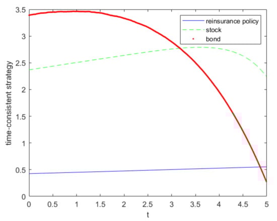
Figure 1. Time consistent reinsurance and investment strategy.

First, we discuss the effects of two basic parameters: $\gamma$ and $r_0$ on the equilibrium reinsurance and investment strategy. By taking derivatives, we have $\frac{\partial {\alpha }^{\pi *}\left(t\right)}{\partial \gamma }=-\frac{{\alpha }^{\pi *}\left(t\right)}{\gamma }<0$, $\frac{\partial {\beta }^{\pi *}\left(t\right)}{\partial \gamma }=-\frac{{\beta }^{\pi *}\left(t\right)}{\gamma }<0$. This means that, as $\gamma$ increases, equilibrium investment in stock and insurance risk exposure will decrease. It is natural because the insurer will buy more reinsurance and buy less stock when they become more risk averse. Figure 2 displays the effects of $\gamma$ and $r_0$ on equilibrium strategy at time 0. We can find that bond investment will increase as $\gamma$ increases, partly because they are a safer asset when compared with stock. Additionally, we have $\frac{\partial {\alpha }^{\pi *}\left(0\right)}{\partial r_0}=-q_2\left(0\right){\alpha }^{\pi *}\left(0\right)<0$, $\frac{\partial {\beta }^{\pi *}\left(0\right)}{\partial r_0}=-q_2\left(0\right){\beta }^{\pi *}\left(0\right)<0$, which is shown in Figure 2. In Figure 2, we can see that ${\gamma }^{\pi *}\left(0\right)$ increases as $r_0$ increases. This means that, as $r_0$ increases, the insurer will prefer risk free asset and bond to stock.

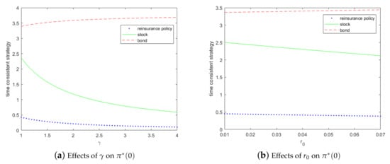
Figure 2. Effects of $\gamma$ and $r_0$ on equilibrium reinsurance and investment strategy (time 0).

Second, we discuss how insurance parameters affect the equilibrium reinsurance strategy. From the expression of ${\alpha }^{\pi *}\left(t\right)$ in Equation (47), we have $\frac{\partial {\alpha }^{\pi *}\left(t\right)}{\partial {\mu }_y}>0$, $\frac{\partial {\alpha }^{\pi *}\left(t\right)}{\partial {\sigma }_y}<0$, $\frac{\partial {\alpha }^{\pi *}\left(t\right)}{\partial \eta }>0$, and $\frac{\partial {\alpha }^{\pi *}\left(t\right)}{\partial {\sigma }_0}<0$. Accordingly, the insurance risk exposure of insurer will become larger as ${\mu }_y$ becomes larger; this is because they can get more income from premium as ${\mu }_y$ increases. However, ${\alpha }^{\pi *}\left(t\right)$ will decrease when ${\sigma }_y$ or ${\sigma }_0$ increases. ${\sigma }_y$ and ${\sigma }_0$ are the volatility of insurance risk. When they become larger, the insurer tends more to reinsurance and transfers the risk to the reinsurer. $\eta$ is the safety loading of reinsurer, when $\eta$ increases, the reinsurance becomes more expensive for the insurer, so they will buy less reinsurance.

Subsequently, we discuss the effects of stock model parameters on ${\beta }^{\pi *}\left(t\right)$. From the expression of ${\beta }^{\pi *}\left(t\right)$, we have:

$$\frac{\partial {\beta }^{\pi *}\left(t\right)}{\partial \kappa }=\frac{-\rho {\sigma }_L{\nu }^2}{\gamma {(\kappa +\rho \nu {\sigma }_L)}^2}\{e^{-(\kappa +\rho \nu {\sigma }_L)(T-t)}[(\kappa +\rho \nu {\sigma }_L)(T-t)+1]-1\}{e}^{-q_1\left(t\right)-q_2\left(t\right)r\left(t\right)}$$

Because $e^{-(\kappa +\rho \nu {\sigma }_L)(T-t)}[(\kappa +\rho \nu {\sigma }_L)(T-t)+1]<1$ always holds when $\kappa +\rho \nu {\sigma }_L\ne 0$, we conclude that: when $\rho >0$, $\frac{\partial {\beta }^{\pi *}\left(t\right)}{\partial \kappa }>0$; when $\rho =0$, $\frac{\partial {\beta }^{\pi *}\left(t\right)}{\partial \kappa }=0$; when $\rho <0$, $\frac{\partial {\beta }^{\pi *}\left(t\right)}{\partial \kappa }<0$. The relations between parameters ${\sigma }_L$, $\nu$, and ${\beta }^{\pi *}\left(t\right)$ are complicated. We give numerical examples in Figure 3; we find that using basic parameters in the paper, ${\beta }^{\pi *}\left(t\right)$ has a positive relation with both ${\sigma }_L$ and $\nu$.

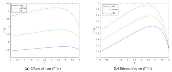
Figure 3. Effects of $\nu$ and ${\sigma }_L$ on ${\beta }^{\pi *}\left(t\right)$.

Figure 4 depicts the impact of initial interest rate $r_0$ and ${\lambda }_r$ on the efficient frontier. We can see that the efficient frontier moves upwards as $r_0$ increases. Insurers tend to invest more in bond and less in stock when $r_0$ increases, and the insurance risk exposure will be smaller. In this case, the variance of the terminal variance will be smaller under the same expected terminal wealth. Efficient frontier also moves upwards as ${\lambda }_r$ becomes larger. This is in accordance with our intuition, because larger ${\lambda }_r$ means more return per unit risk.

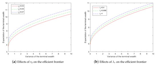
Figure 4. Effects of $r_0$ and ${\lambda }_r$ on the efficient frontier.

6. Conclusions

In this paper, we investigate a mean-variance investment and reinsurance problem in a stochastic interest rate and stochastic volatility framework. The surplus process is modelled by the jump-diffusion process. The insurer can purchase reinsurance or acquire new business and invest in a risk-free asset, stock, and bond. The dynamic of interest rate is modelled by Vasicek model, while the stock price follows the Heston model. We tackle the problem in a game-theoretic perspective in order to overcome time-inconsistency. First, we provide a verification theorem for the problem. Subsequently, we solve the extended HJB equations explicitly and obtain the equilibrium investment and reinsurance strategies. We find that the time-consistent investment in bond will depend on wealth level, because the bond here plays a similar role that the risk free asset plays in the constant interest rate case. We also find that time-consistent investment in stock and insurance risk exposure will depend on the interest rate and not depend on the level of stochastic volatility. Finally, we analyze the impact of model parameters on time-consistent strategies and efficient frontier.

Our model has several limitations, for example, the reinsurance proportion is allowed to be greater than one. It is more realistic to limit the reinsurance proportion to $[0,1]$. However, in this way, we cannot get a closed form solution, because the equilibrium reinsurance strategy depends on the stochastic interest rate. Perhaps we can use the numerical method to solve this problem and we left it for future research. Our model can also be extended in following ways: (1) we can consider time-consistent robust control based on our model assuming that the insurer is ambiguity-averse. (2) We can consider the insurer with an incomplete observation due to the fact that financial market information usually cannot be fully obtained. (3) The stock model and interest rate model can be extended to a more sophisticated case. However, these extensions may lead to new technical difficulties; we also left them for future research.

References

- Browne, S. Optimal investment policies for a firm with a random risk process: Exponential utility and minimizing the probability of ruin. Math. Oper. Res. 1995, 20, 937–958. [Google Scholar] [CrossRef]
- Yang, H.; Zhang, L. Optimal investment for insurer with jump-diffusion risk process. Insur. Math. Econ. 2005, 37, 615–634. [Google Scholar] [CrossRef]
- Schmidli, H. On minimizing the ruin probability by investment and reinsurance. Ann. Appl. Probab. 2002, 12, 890–907. [Google Scholar] [CrossRef]
- Bai, L.; Guo, J. Optimal proportional reinsurance and investment with multiple risky assets and no-shorting constraint. Insur. Math. Econ. 2008, 42, 968–975. [Google Scholar] [CrossRef]
- Li, D.; Zeng, Y.; Yang, H. Robust optimal excess-of-loss reinsurance and investment strategy for an insurer in a model with jumps. Scand. Actuar. J. 2018, 2018, 145–171. [Google Scholar] [CrossRef]
- Guan, G.; Liang, Z. Optimal reinsurance and investment strategies for insurer under interest rate and inflation risks. Insur. Math. Econ. 2014, 55, 105–115. [Google Scholar] [CrossRef]
- Zhang, X.; Meng, H.; Zeng, Y. Optimal investment and reinsurance strategies for insurers with generalized mean-variance premium principle and no-short selling. Insur. Math. Econ. 2016, 67, 125–132. [Google Scholar] [CrossRef]
- Liang, X.; Young, V.R. Minimizing the probability of ruin: Two riskless assets with transaction costs and proportional reinsurance. Stat. Probab. Lett. 2018, 140, 167–175. [Google Scholar] [CrossRef]
- Markowitz, H. Portfolio selection. J. Financ. 1952, 7, 77–91. [Google Scholar]
- Zhou, X.Y.; Li, D. Continuous-time mean-variance portfolio selection: A stochastic LQ framework. Appl. Math. Opt. 2000, 42, 19–33. [Google Scholar] [CrossRef]
- Bäuerle, N. Benchmark and mean-variance problems for insurers. Math. Method Oper. Res. 2005, 62, 159–165. [Google Scholar] [CrossRef]
- Bai, L.; Zhang, H. Dynamic mean-variance problem with constrained risk control for the insurers. Math. Method Oper. Res. 2008, 68, 181–205. [Google Scholar] [CrossRef]
- Bi, J.; Guo, J. Optimal mean-variance problem with constrained controls in a jump-diffusion financial market for an insurer. J. Optimiz. Theory Appl. 2013, 157, 252–275. [Google Scholar] [CrossRef]
- Shen, Y.; Zhang, X.; Siu, T.K. Mean-variance portfolio selection under a constant elasticity of variance model. Oper. Res. Lett. 2014, 42, 337–342. [Google Scholar] [CrossRef]
- Björk, T.; Murgoci, A.; Zhou, X.Y. Mean-variance portfolio optimization with state-dependent risk aversion. Math. Financ. 2014, 24, 1–24. [Google Scholar] [CrossRef]
- Björk, T.; Khapko, M.; Murgoci, A. On time-inconsistent stochastic control in continuous time. Financ. Stoch. 2017, 21, 331–360. [Google Scholar] [CrossRef]
- Zeng, Y.; Li, Z. Optimal time-consistent investment and reinsurance policies for mean-variance insurers. Insur. Math. Econ. 2011, 49, 145–154. [Google Scholar] [CrossRef]
- Zeng, Y.; Li, Z.; Lai, Y. Time-consistent investment and reinsurance strategies for mean-variance insurers with jumps. Insur. Math. Econ. 2013, 52, 498–507. [Google Scholar] [CrossRef]
- Zhao, H.; Shen, Y.; Zeng, Y. Time-consistent investment-reinsurance strategy for mean-variance insurers with a defaultable security. J. Math. Anal. Appl. 2016, 437, 1036–1057. [Google Scholar] [CrossRef]
- Xiao, H.; Ren, T.; Bai, Y.; Zhou, Z. Time-Consistent Investment-Reinsurance Strategies for the Insurer and the Reinsurer under the Generalized Mean-Variance Criteria. Mathematics 2019, 7, 857. [Google Scholar] [CrossRef]
- Zhu, J.; Guan, G.; Li, S. Time-consistent non-zero-sum stochastic differential reinsurance and investment game under default and volatility risks. J. Comput. Appl. Math. 2020, 374, 112737. [Google Scholar] [CrossRef]
- Heston, S.L. A closed-form solution for options with stochastic volatility with applications to bond and currency options. Rev. Financ. Stud. 1993, 6, 327–343. [Google Scholar] [CrossRef]
- Li, Z.; Zeng, Y.; Lai, Y. Optimal time-consistent investment and reinsurance strategies for insurers under Heston’s SV model. Insur. Math. Econ. 2012, 51, 191–203. [Google Scholar] [CrossRef]
- Liu, J. Portfolio selection in stochastic environments. Rev. Financ. Stud. 2007, 20, 1–39. [Google Scholar] [CrossRef]
- Yan, T.; Han, B.; Pun, C.S.; Wong, H.Y. Robust time-consistent mean-variance portfolio selection problem with multivariate stochastic volatility. Math. Financ. Econ. 2020, 14, 699–724. [Google Scholar] [CrossRef]
- Ahlip, R.; Rutkowski, M. Pricing of foreign exchange options under the Heston stochastic volatility model and CIR interest rates. Quant. Financ. 2013, 13, 955–966. [Google Scholar] [CrossRef]
- Guan, G.; Liang, Z. Optimal management of DC pension plan in a stochastic interest rate and stochastic volatility framework. Insur. Math. Econ. 2014, 57, 58–66. [Google Scholar] [CrossRef]
- Li, D.; Rong, X.; Zhao, H. Time-consistent reinsurance-investment strategy for a mean-variance insurer under stochastic interest rate model and inflation risk. Insur. Math. Econ. 2015, 64, 28–44. [Google Scholar] [CrossRef]
- Korn, R.; Kraft, H. A stochastic control approach to portfolio problems with stochastic interest rates. SIAM J. Control Optim. 2002, 40, 1250–1269. [Google Scholar] [CrossRef]
- Pan, J.; Xiao, Q. Optimal asset-liability management with liquidity constraints and stochastic interest rates in the expected utility framework. J. Comput. Appl. Math. 2017, 317, 371–387. [Google Scholar] [CrossRef]
- Wei, J.; Wang, T. Time-consistent mean-variance asset-liability management with random coefficients. Insur. Math. Econ. 2017, 77, 84–96. [Google Scholar] [CrossRef]
- Mao, X. Stochastic Differential Equations and Applications; Elsevier: Amsterdam, The Netherlands, 2007. [Google Scholar]
- Escobar, M.; Neykova, D.; Zagst, R. HARA utility maximization in a Markov-switching bond-stock market. Quant. Financ. 2017, 17, 1715–1733. [Google Scholar] [CrossRef]
Publisher’s Note: MDPI stays neutral with regard to jurisdictional claims in published maps and institutional affiliations. |
© 2020 by the authors. Licensee MDPI, Basel, Switzerland. This article is an open access article distributed under the terms and conditions of the Creative Commons Attribution (CC BY) license (http://creativecommons.org/licenses/by/4.0/).