Abstract
A correlation analysis of pollutant variables provides comprehensive information on dependency behaviour and is thus useful in relating the risk and consequences of pollution events. However, common correlation measurements fail to capture the various properties of air pollution data, such as their non-normal distribution, heavy tails, and dynamic changes over time. Hence, they cannot generate highly accurate information. To overcome this issue, this study proposes a combination of the Generalized Autoregressive Conditional Heteroskedasticity model, Generalized Pareto distribution, and stochastic copulas as a tool to investigate the dependence structure between the PM10 variable and other pollutant variables, including CO, NO2, O3, and SO2. Results indicate that the dynamic dependence structure between PM10 and other pollutant variables can be described with a ranking of PM10–CO > PM10–SO2 > PM10–NO2 > PM10–O3 for the overall time paths (δ) and the upper tail (τU) or lower tail (τL) dependency measures. This study reveals an evident correlation among pollutant variables that changes over time; such correlation reflects dynamic dependency.
1. Introduction
The air pollution problem has long been the centre of discussions all over the world. This issue is particularly alarming for the urban areas of developed and developing countries [1,2,3]. In Malaysia, air pollution is generally determined from five major types of pollutants, namely, carbon monoxide (CO), suspended particulate matter (PM10), sulphur dioxide (SO2), ozone (O3), and nitrogen dioxide (NO2) [4,5]. These five pollutant variables are observed simultaneously and monitored constantly to provide relevant information about air quality [6]. As these pollutants are simultaneously being observed and monitored, the investigation into the relationship and correlation among these five pollutant variables is expected to contribute to a comprehensive understanding of the behaviour of air pollution events at any particular area. For example, Marković et al. [7] have investigated the behaviour of CO, O3, NO2, SO2, and PM10 in the Belgrade urban area during the autumnal period of 2005. They reported the existence of a positive correlation between the PM10 SO2, NO2, and CO. On the contrary, the O3 variable was found to indicate a negative correlation with SO2, NO2, PM10 and CO. With the basis of the correlation measured, they contended that SO2, NO2, CO, and PM10 could originate from similar sources. Rich et al. [8] found a high association between myocardial infarction disease and particulate matter concentration in the presence of other pollutants, such as O3, CO, SO2, and NO2. The analysis by Xie et al. [9] for 31 Chinese cities showed the following: the correlation between particulate matter and NO2 and SO2 is either high or moderate, the correlation between particulate matter and CO is diverse, and the correlation between particulate matter and O3 is either weak or uncorrelated. These results varied spatio-temporally across all the cities.
Generally, the dependency between two or more pollutant variables is measured by the Pearson, Spearman, or Kendall correlation methods. These common methods are widely popular because of their computational simplicity and easily interpretable results. However, despite their simplicity, the Pearson correlation method can only measure the strength of the linear dependence between the underlying random variables. In fact, the Pearson correlation method fails to provide an accurate measurement if any of the variables involved do not follow a normal distribution [10,11]. Unfortunately, the distribution of air pollutant data rarely follows a normal distribution. Instead, they often follow fat tailed distributions, such as the extreme value distribution, especially during periods of extreme pollution events [12,13,14]. However, the empirical measure of the Spearman or Kendall correlation method provides rank correlation measures which do not consider the properties of marginal distributions and time-varying properties among the random variables.
Apart from the common methods, several studies have considered a long-memory approach to investigate the temporal relationship and dependency behaviour of air pollutant data [15]. For example, Lee [16] showed the existence of scale-invariant behaviour in the air pollution concentration time series based on the concept of multifractal characteristics and long-term memory. Weng et al. [17] found that the time series of the ozone in Southern Taiwan indicates a long and persistent memory process involving nonlinearity and fractal time series based on R/S analyses. In a similar vein, Liu et al. [18] have shown the existence of persistence in the time-scaling behaviour for three pollution indices (SO2, PM10, NO2) in Shanghai, China, using the method of detrended fluctuation analysis (DFA) and the multifractal approach. However, these methods are bound by some limitations. Particularly, they fail to integrate the behaviour of asymmetric co-movements and contagion effects that exist in the dynamic behaviour among variables. The existence of this behaviour could affect the results of the analysis [19]. Thus, to overcome this problem, the method of dynamic conditional correlation (DCC) proposed by Engle [20] and Engle and Colacito [21] seems to be a good alternative. However, the data indicate the existence of extreme values and long tail properties; hence, an asymmetrical measure of a tail correlation may lead to biased estimates in DCC models [22,23].
As the probabilistic behaviour of extreme events can be effectively described using extreme value models, such as the generalized Pareto distribution (GPD), this study proposes a combination of a GPD model with copulas to establish a model that is able to describe the dependence structure between the PM10 variable and a set of four major pollutant variables, namely, CO, NO2, SO2, and O3. This study adopts the copula approach because it is flexible to use with various types of marginal distributions without being constrained by normality limitations. A copula model can easily provide accurate information on the joint distribution of several pollution variables. The Gaussian copula was used in this study to describe the behaviour of the dependence structure among the pollutant variables. To investigate the tail dependence among the pollutant variables, this work employed the symmetrized Joe–Clayton (SJC) copulas. The generalized autoregressive conditional heteroskedasticity (GARCH) model was also combined with the GPD model to improve the distribution modelling. This combination method integrates all the properties of fat tail behaviour, asymmetric co-movements, stochastic volatility, as well as the contagion effects that exist on the dynamic behaviour among variables.
2. Study Area and Data
Klang is a large city in Malaysia located at a latitude of 101°26′44.023′′ E latitude and 3°2′41.701′′ N longitude. Klang is characterized by a dense population and an area of approximately 573 km2. It is the centre of the import and export activities in Malaysia. Various important industrial, commercial, and economic activities are carried out in Klang. Moreover, Klang has been recognized as the 16th busiest container port and the 13th busiest trans-shipment port in the world [24]. However, its rapid urbanization has increased its risk of atmospheric pollution. Thus, given the importance of Klang, the behaviour of the air pollutants in the region should be evaluated and analysed. Figure 1 shows the location of Klang in peninsular Malaysia.
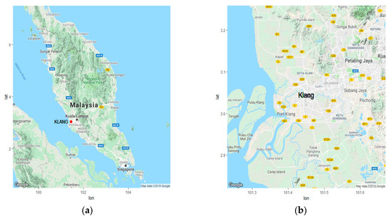
Figure 1.
(a) Map of peninsular Malaysia (the location of Klang is marked by the red dotted point); and (b) map of Klang.
This study used the daily data of five main pollutant variables, namely, SO2, NO2, CO, PM10, and O3 for the period 1 January 2002–31 December 2016. A small percentage of missing values with a random pattern were found in the data. Thus, the single imputation method based on the average of the last known and next known observations was used to estimate the missing data. In addition to its easy implementation, the method provides satisfactory results for missing data with a random mechanism [25].
3. Generalized Pareto Distribution (GPD) Model
Extreme events are generally rare events that occur in the upper or lower tails of the distribution of data. Meanwhile, the extreme pollution data refer to an environment with a large air pollution index (API) at particular periods. represent the independent and identically distributed random variables of the hourly pollutants. The distribution of is governed by an unknown density function F. High value pollutant variables that exceed the unhealthy level (≥100) indicate a pollution event. Mathematically, this phenomenon could represent a conditional event that is larger than some threshold u, and its conditional exceedance distribution function can be written as follows:
The extreme value approach is also known as the peaks-over-threshold method and is used for events with a threshold of u [26]. In this study, the observed excesses over the threshold are fitted to the GPD given by the following equation:
where . The parameters and refer to the shape and scale parameter, respectively [27].
4. Generalized Autoregressive Conditional Heteroskedasticity (GARCH) Model
The GJR–GARCH model was used as a marginal distribution for each pollutant variable. Let represent the time series data for the pollutant variables, and let denote the conditional variance for the period of t. Then, the GJR–GARCH model can be written as
where when is negative and 0 otherwise. Then, df denotes the degree of freedom, and represents the previous time data by t−1. Then, the standardize residual of the series can be described as a t-distribution given as
The GDP model is used to model the tail behaviour in the distribution of each pollutant variable. In sum, our approach is a combination of the GJR–GARCH and GPD models. The GJR–GARCH model is used to describe the interior part of the marginal distribution for each pollutant variable while the GPD model is used to describe the tail behaviour of each pollutant variable. In this study, we used the 10th percentile as the lower threshold to indicate a healthy air environment and the 90th percentile as the upper threshold to indicate an unhealthy air environment. Thus, the combination of the GJR–GARCH and GPD models can be represented as the following cumulative function:
where n is the sample size of the data, represents the volume of data below the threshold and represents the volume of data above the threshold , represents the distribution function determined from the GJR–GARCH model, and is the number of observations below (exceeding) the threshold .
5. Copula Model
A copula model can be used to provide accurate information about the joint distribution of several pollution variables because it is not tied to the assumption of normality for the datasets involved. Moreover, the ability of the copula model to extract information regarding the dependence structure from the joint probability distribution function makes it a useful method for air pollution modelling. Mathematically, for a couple of random variables and , a bivariate copula model can be determined as
where C is the copula function; and and , are the marginal distributions of the random variables and , respectively [10]. In this study, a Gaussian model was used to describe the overall dependence structure between the pollutant variables. The SJC copula is used to describe the behaviour of the dependence structure for the upper and lower tails of each pollutant variable.
6. Interrelationship Behaviour among Pollutant Variables
To evaluate the interrelationship behaviour among the pollutant variables, we use a time-varying model for the Gaussian and SJC copulas.
6.1. Gaussian Copula
The Gaussian copula is a well known copula that has been used in applied research. It is associated with a multivariate normal distribution. For a bivariate distribution, which involves random variables u and v, its dependence structure based on the Gaussian copula can be determined as
with:
where is the linear correlation coefficient and is the standard normal cumulative density function. To include the time-varying properties, Patton [28] proposed a modification on the Gaussian dependence parameter by assuming that it evolves over time; the modified parameter is given as
where is the modified logistic transformation that ensures in the interval of (−1, 1). The parameter of plays a roles to capture the persistence effect while the mean of the model for the 10 observations of the transformed variables and represents the variation effect of the dependence series.
6.2. SJC Copula
The SJC copula is determined from the modification of the Joe–Clayton copula. The Joe–Clayton copula is given as
where
The terms and represent the upper tail dependence and lower tail dependence, respectively. However, the Joe–Clayton copula cannot be used to evaluate the behaviour of the upper and lower tail dependence simultaneously. Thus, the SJC copula is used herein to overcome the weakness of the Joe–Clayton copula. The SJC copula is given as
where represents the Joe–Clayton copula in Equation (11). To include the time-varying properties, Patton [28] proposed the use of the evolution parameters in the SJC copula; the formula is written as follows:
where is the logistic transformation obtained as ; it ensures that the dependence parameter is in the range of (0, 1). Equation (15) specifies that follows the Autoregressive-Moving Average (ARMA) type process with the order of (1,10), in which represents the autoregression, is the forcing variable and represents the persistence effect and variation in dependence.
The parameters for each model are estimated by a two-step estimation procedure. First, the parameters of the GARCH model corresponding to the GPD model for the upper and lower tails are estimated, and the standardized residuals are determined. Second, a transformation is performed using the distribution functions to create pseudo-uniform variables. On the basis of these pseudo-uniform variables, a copula model is estimated by maximizing the log-likelihood function given by
where represents the parameter vector for each copula model, for i = 1,2, and k = 1,3,…, K [29,30].
7. Results and Discussion
A preliminary statistical analysis was carried out prior to the detailed discussion of the analysis results. Figure 2 shows that the volatility of PM10 is higher than those of the other pollutant variables. Table 1 presents the descriptive statistics of all pollutant variables. The mean and median for PM10 were found to be higher than those of the other pollutant variables. Hence, this pollutant exerts the greatest influence on the status of air quality. In addition, the standard deviation of PM10 is the highest among all variables, thus implying that PM10 presents more volatile behaviour than the other pollutant variables. NO2 shows the lowest standard deviation and thus exhibits the most stable dynamic behaviour. The PM10 pollutant also shows the highest of kurtosis value, which indicates that it appears most frequently in unhealthy pollution events. All the pollutant variables were found to have a positive skewness. A high positive skewness means that the pollutants exhibit long tailed behaviour to the right of the distribution data. The Jarque–Bera test results confirm that all the pollutant variables are not normally distributed. In particular, high Jarque–Bera test statistics are found for PM10 and SO2. The results in Table 1 indicate that all the pollutant variables exhibit a nonlinear phenomenon and extreme behaviour. Thus, a model that functions under the normality assumption is not appropriate to use in representing these types of data.
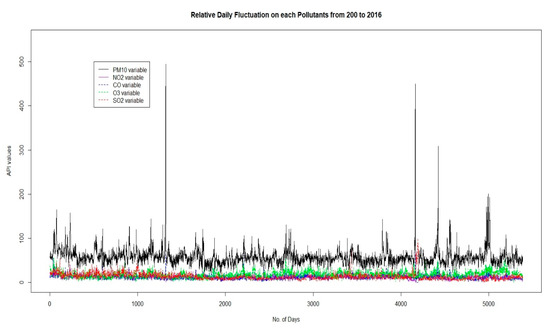
Figure 2.
Time series plot for the relative daily fluctuation of each pollutant variable.

Table 1.
Descriptive statistics for datasets 1, 2, 3 and 4.
Table 2 shows the results of the correlation among all the pollutant variables. The linear correlation values for the PM10 pollutant in relation to the other pollutants range from −0.077 to 0.684. The PM10 pollutant-related pairs are strongly correlated with CO, followed by O3, NO2, and SO2. The NO2 pollutant is found to have a moderate correlation with the CO pollutant. For the other pairs of pollutant variables, they present a positive low correlation. However, the measurement of linear correlation may generate misleading results because it assumes that the pairs of data share linearity properties. Moreover, linear correlation measures generally work well for pairs of data that satisfy a normality assumption. For most air pollutant data, the existence of skewness cannot be neglected, as presented in the results in Table 1. A linear correlation measure also indicates a constant correlation behaviour over time for each pollutant variable. However, one of the most important characteristics of air pollution data is that they always fluctuate with volatility behaviour over time. Particularly during unhealthy air pollution events, some of the pollution variables can increase significantly and thereby correspond to extreme values. These behaviours are clearly depicted in Figure 2. Thus, we believe that a linear correlation measure may not be a reliable tool for describing the relationship among pollutant variables. As mentioned previously, we address these issues by proposing a time-varying copula with a combination of the GPD and GARCH models.
Table 2.
Correlation among the pollutant variables.
In the analysis, the parameters for the tails of each pollutant variable are estimated on the basis of the GPD model. Table 3 shows the estimated parameters describing the upper and lower tail behaviour of the data of each pollutant variable. The sign of the shape parameter shows how fast the tail decreases. A negative value indicates that the tail is finite, whereas a positive value indicates that the tail decreases as a polynomial. The higher the absolute value of the shape parameter is, the heavier the tail distribution will be. As shown in Table 3, for the lower tails, all pollutant variables are found to have a negative estimate of parameter ξ. This result indicates that all pollution variables exhibit finite short tail behaviour, with the PM10 pollutant exhibiting the lowest value of ξ (−0.0626). For the upper tails, the CO, NO2, and SO2 pollutants exhibit short tail behaviour. The PM10 pollutant is found to have the highest positive value ξ = 0.1142, followed by the SO2 pollutant with ξ = 0.0179. These values indicate that the PM10 and SO2 pollutants demonstrate heavy upper tail behaviour. These results indicate that all pollutant variables present the same pattern for a low API at a particular time. In the case of extreme pollution events, the PM10 variable is most likely to have the highest API value among all pollution variables at a particular time. Hence, the PM10 pollutant is highly volatile, particularly at the upside of its distribution.
Table 3.
Correlation among pollutant variables.
Figure 3 shows a comparison of the empirical and GPD plots for the cumulative distribution function (CDF) of the exceedance of the residuals in the upper tail of each pollutant variable. The fitted GPD closely follows the exceedance of the residuals, although only 10% of the standardized residuals were employed. Thus, the GPD model is a suitable choice for the upper tail data of each pollutant. This result is also valid for the lower tails. On the basis of the GPD model, the overall CDF of the semi-parametric models is obtained (Figure 4). In particular, the lower and upper tails are determined by the fitted GPD model while the interior part is estimated by the GARCH model.
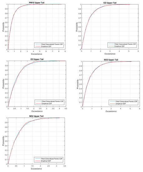
Figure 3.
Fitted generalized Pareto distribution (GPD) model of the upper tail distributions for each pollutant variable.
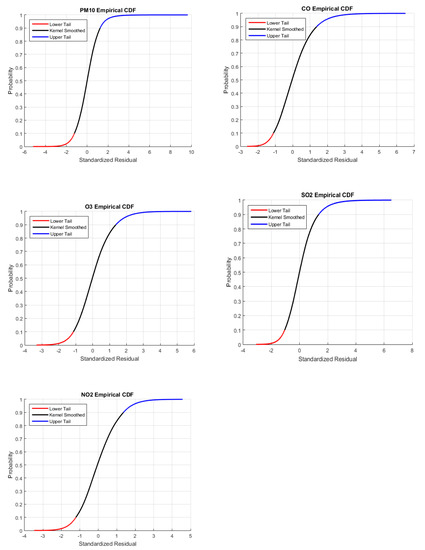
Figure 4.
Fitted semi-parametric models for each pollutant variable.
The results shown in Table 3 and Figure 3 and Figure 4 demonstrate that our approach can adequately model the marginal distributions of the time series data of the air pollutant variables in Malaysia. However, the estimated marginal distribution alone is not able to describe the dependence structure that exists among the pollutant variables. Thus, a copula needs to be adopted in the model. As mentioned previously, the Gaussian and SJC copulas are employed in this study. Given the available properties on each copula model, the Gaussian copula is useful in assessing the overall dependence structure of pollutant variables, as described in Equation (10). For the SJC copula model, it is useful in exploring the dependence behaviour of the lower and upper tails, as described in Equations (14) and (15).
Table 4 shows the results of the parameter estimates for the Gaussian and SJC copulas. The most important parameters for the constant copula are determined by δ for the Gaussian copula and by the and parameters for the SJC copula. For the time-varying copulas, the important parameters for the Gaussian copula are ω, α, and β; and those for the SJC copula are , , , , and . As shown in Table 3, the PM10 variable is likely to have the highest API value among all pollution variables at a particular time. Thus, investigating the dynamic dependency of PM10 on other pollutant variables could yield informative results. In this regard, the parameters of , , and are useful in describing the magnitude of dependence between PM10 and other pollutant variables. The adjustment in the dependence measure is captured by the parameters of , and . Moreover, the parameters , and are useful to represent the degree of the persistence of the dependence.
Table 4.
Parameter estimates for constant and time-varying copulas.
The best fitting copula model is determined by goodness-of-fit measures, namely, Akaike’s information criterion (AIC) and Bayesian information criterion (BIC). The lowest value determined by the AIC or BIC indicates a well fitted model (Table 4). Two important points can be derived from the information provided in Table 4 and Figure 5, Figure 6, Figure 7 and Figure 8. First, the overall dependence (δ) between PM10 and the other pollutants can be ranked in decreasing order as PM10–CO > PM10–SO2 > PM10–NO2 > PM10–O3. Second, the rank in decreasing order for the upper tail () and lower tail () dependence between PM10 and the other pollutants is found to be same as that of the overall dependence, that is, PM10–CO > PM10–SO2 > PM10–NO2 > PM10–O3. This ranking implies that the dynamic fluctuations between PM10 and CO over time have the strongest overall dependency and tail dependency; they are followed by the relationship of PM10 with SO2 and by PM10 with NO2. The weakest overall dependency and tail dependency are those between PM10 and O3. Thus, we can conclude that CO has the greatest influence on the behaviour of PM10 among all the pollutants in a normal air quality, good air quality (lower tail), or bad air quality (upper tail). The results in Table 4 also show that the value of is larger than that of for all possible pairs. Hence, the upper tail dependency between PM10 and the other pollutants is stronger than the lower tail dependency.
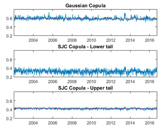
Figure 5.
Dependence path of the time-varying copula for PM10–CO.
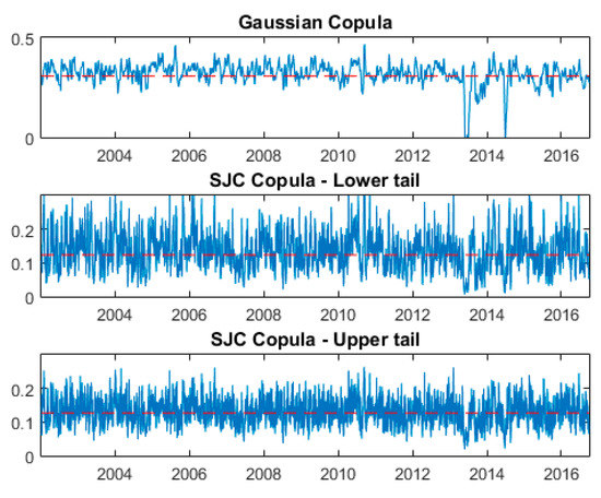
Figure 6.
Dependence path of the time-varying copula for PM10–NO2.
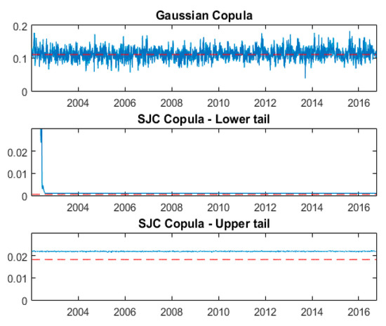
Figure 7.
Dependence path of the time-varying copula for PM10–O3.
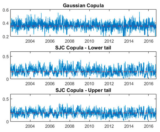
Figure 8.
Dependence path of the time-varying copula for PM10–SO2.
To further investigate the dynamic dependence structure among the pollutant variables, we present in Figure 5, Figure 6, Figure 7 and Figure 8 the time paths for the overall, lower, and upper tail dependencies based on the Gaussian and SJC time-varying copulas. In each figure, the red dashed line denotes the dependence parameter for the constant copula while the solid blue line denotes the dynamic parameter values under the time-varying copula. As mentioned previously, the time variations of the dependency measures between the pollutant variables are described by the parameters of , ,, , and . Then, as shown in Table 4, the results of the time-varying Gaussian copula model reveal that most of the time paths are close to a white noise series as the values of the variation coefficient α are relatively higher than those of the persistence coefficient β, except for the PM10–NO2 relationship. For the time-varying SJC copula, all the persistence coefficients β are larger than the coefficients α for all pairs. This result gives some insights into the changes of the dependence structure for the upper and lower tails over a time period.
For the PM10–CO pair (Figure 5), the parameters realized for the overall time-varying () dependence are found to be in the mean of 0.6 and range of 0.5–0.7. For a lower tail dependence, the time-varying parameters () fluctuate around the mean of 0.35 and range from 0.2 to 0.4. For an upper tail dependence, the time-varying parameters () fluctuate around the mean of 0.42 and range from 0.39 to 0.42. The volatility properties of the time-varying parameters of the upper tail dependence are more stable than those of the overall and lower tail dependencies. They fluctuate around the mean of 0.6 and range from 0.5 to 0.7. Thus, the overall time-varying dependence for PM10–CO is quite high. For the lower tail and upper tail, their time-varying dependencies are relatively moderate. The dependence path of the time-varying copula for PM10–NO2 is shown in Figure 6. The overall time-varying properties of the dependence parameters () are found to be in the range of 0 to 0.5 with a mean of 0.35. Meanwhile, the time-varying lower dependence () fluctuates between 0 and 0.3 with a mean of 0.13. The time-varying upper dependence () fluctuates between 0.02 and 0.25 with a mean of 0.12. The fluctuations of the lower and upper dependency behaviour are more volatile than those of the overall time-varying dependence parameters (). Thus, we can conclude that the time-varying overall, lower tail, and upper tail dependencies for PM10–NO2 are low.
As mentioned previously, Figure 7 shows the dependence path of the time-varying copula for the PM10–O3 pair. The overall dependence parameters () are found to be more volatile than those of the time-varying lower dependence () and upper dependence (). The values of the parameter fluctuate around the mean of 0.12 within a range of 0.05–0.19. The parameters for the time-varying lower dependence () and upper dependence () fluctuate around a very low mean and very low range, except for some early points of the lower tail dependency before the year 2004. However, in general, these values are considerably lower than those for the PM10–CO and PM10–NO2 pairs. Thus, we can conclude that the behaviour of the time-varying overall, lower tail, and upper tail dependencies for PM10–O3 are low. The dependency behaviour of the PM10–NO2 pair is shown in Figure 8. The values of the time-varying overall dependence parameter (), lower dependence (), and upper dependence () indicate similar volatilities in the range of 0–0.5. The mean of the overall dependence parameter is about 0.36, which is higher than the mean of the lower and upper dependence parameters. These values indicate the low magnitudes of the overall, lower tail, and upper tail dependencies for the PM10–NO2 pair. The results shown in Figure 5, Figure 6, Figure 7 and Figure 8 also show that the measure based on the constant copula (red dashed line) is not sufficient to describe the dependency behaviour among the pollutant variables over time. Nevertheless, the constant measure of dependency is found to provide a good approximation of the means of the fluctuations of the plots for overall dependence, lower tail dependence, or upper tail dependence (except for the lower and upper tails of PM10–O3 pair).
8. Conclusions
This study investigated the behaviour of the dynamic dependence structure between several important pollutant variables, namely, PM10, CO, O3, NO2, and SO2. The distribution of each pollutant variable is non-normal, heavy tailed, and dynamically changes over time. Thus, a measurement determined by a common linear method, such as a Pearson correlation, which is subject to the normality assumption, will fail to provide accurate results. The Pearson correlation method is a rigid approach and cannot be used to evaluate the dynamic changes of the dependency behaviour among pollutant variables over time. Thus, this study proposes a method that combines the GARCH, GPD, and copula models to overcome air pollution data’s non-normal, heavy tailed, and dynamically changing properties over time. The results in this work indicate that compared with the linear correlation method, the proposed method provides more information about the behaviour of the dependency structure among pollutant variables, particularly in terms of the overall time paths and lower and upper tail dependencies.
Author Contributions
Conceptualization, formal analysis, investigation, methodology and writing, funding acquisition, review and editing, N.M.; software, review and editing, S.I.H. All authors have read and agreed to the published version of the manuscript.
Funding
This work is supported by the Universiti Kebangsaan Malaysia (grant number FRGS/1/2014/SG04/UKM/03/1 and DIP-2018-038).
Acknowledgments
The authors would like to thank the editor for their time spent on reviewing our manuscript. The authors would also like to thank the reviewers for the careful and insightful review of our manuscript.
Conflicts of Interest
The authors declared no potential conflicts of interest with respect to the research.
References
- Torres, J.M.; Pérez, J.P.; Val, J.S.; McNabola, A.; Comesaña, M.M.; Gallagher, J. A functional data analysis approach for the detection of air pollution episodes and outliers: A case study in Dublin, Ireland. Mathematics 2020, 8, 225. [Google Scholar] [CrossRef]
- Mannucci, P.M.; Franchini, M. Health effects of ambient air pollution in developing countries. Int. J. Environ. Res. Public Health 2017, 14, 1048. [Google Scholar] [CrossRef] [PubMed]
- Masseran, N. Modeling fluctuation of PM10 data with existence of volatility effect. Environ. Eng. Sci. 2017, 34, 816–827. [Google Scholar] [CrossRef]
- AL-Dhurafi, N.A.; Masseran, N.; Zamzuri, Z.H. Compositional time series analysis for air pollution index data. Stoch. Environ. Res. Risk Assess. 2018, 32, 2903–2911. [Google Scholar] [CrossRef]
- AL-Dhurafi, N.A.; Masseran, N.; Zamzuri, Z.H. Hierarchical-Generalized Pareto model for estimation of unhealthy air pollution index. Environ. Model. Assess. 2020, 25, 555–564. [Google Scholar] [CrossRef]
- Department of Environment. A Guide to Air Pollutant Index in Malaysia (API); Ministry of Science, Technology and the Environment: Kuala Lumpur, Malaysia, 1997.
- Marković, D.M.; Marković, D.A.; Jovanović, A.; Lazić, L.; Mijić, Z. Determination of O3, NO2, SO2, CO and PM10 measured in Belgrade urban area. Environ. Monit. Assess. 2008, 145, 349–359. [Google Scholar] [CrossRef]
- Rich, D.Q.; Ozkaynak, H.; Crooks, J.; Baxter, L.; Burke, J.; Ohman-Strickland, P.; Thevenet-Morrison, K.; Kipen, H.M.; Zhang, J.; Kostis, J.B.; et al. The triggering of myocardial infarction by fine particles is enhanced when particles are enriched in secondary species. Environ. Sci. Technol. 2013, 47, 9414–9423. [Google Scholar] [CrossRef]
- Xie, Y.; Zhao, B.; Zhang, L.; Luo, R. Spatiotemporal variations of PM2.5 and PM10 concentrations between 31 Chinese cities and their relationships with SO2, NO2, CO and O3. Particuology 2015, 20, 141–149. [Google Scholar] [CrossRef]
- Hofert, M.; Kojadinovic, I.; Machler, M.; Yan, J. Elements of Copula Modeling with R; Springer: Cham, Switzerland, 2018. [Google Scholar]
- Cherubini, U.; Mulinacci, S.; Gobbi, F.; Romagnoli, S. Dynamic Copula Methods in Finance; Wiley: West Sussex, UK, 2011. [Google Scholar]
- AL-Dhurafi, N.A.; Masseran, N.; Zamzuri, Z.H.; Safari, M.A.M. Modeling the air pollution index based on its structure and descriptive status. Air Qual. Atmos. Health 2018, 11, 171–179. [Google Scholar] [CrossRef]
- Masseran, N.; Safari, M.A.M. Risk assessment of extreme air pollution based on partial duration series: IDF approach. Stoch. Environ. Res. Risk Assess. 2020, 34, 545–559. [Google Scholar] [CrossRef]
- Masseran, N.; Safari, M.A.M. Intensity–duration–frequency approach for risk assessment of air pollution events. J. Environ. Manag. 2020, 264, 110429. [Google Scholar] [CrossRef] [PubMed]
- Chelani, A. Long-memory property in air pollutant concentrations. Atmos. Res. 2016, 171, 1–4. [Google Scholar] [CrossRef]
- Lee, C.-K. Multifractal characteristics in air pollutant concentration time series. Water Air Soil Pollut. 2002, 135, 389–409. [Google Scholar] [CrossRef]
- Weng, Y.-C.; Chang, N.-B.; Lee, T.Y. Nonlinear time series analysis of ground-level ozone dynamics in Southern Taiwan. J. Environ. Manag. 2008, 87, 405–414. [Google Scholar] [CrossRef] [PubMed]
- Liu, Z.; Wang, L.; Zhu, H. A time–scaling property of air pollution indices: A case study of Shanghai, China. Atmos. Pollut. Res. 2015, 6, 886–892. [Google Scholar] [CrossRef]
- Poon, S.H.; Rockinger, M.; Tawn, J. Extreme value dependence in financial markets: Diagnostics, models, and financial implications. Rev. Financ. Stud. 2004, 17, 581–610. [Google Scholar] [CrossRef]
- Engle, R. Dynamic conditional correlation: A simple class of multivariate generalized autoregressive conditional heteroskedasticity models. J. Bus. Econ. Stat. 2002, 20, 339–350. [Google Scholar] [CrossRef]
- Engle, R.; Colacito, R. Testing and valuing dynamic correlations for asset allocation. J. Bus. Econ. Stat. 2006, 24, 238–253. [Google Scholar] [CrossRef]
- Silvennoinen, A.; Teräsvirta, T. Modeling multivariate autoregressive conditional heteroskedasticity with the double smooth transition conditional correlation GARCH model. J. Financ. Econom. 2009, 7, 373–411. [Google Scholar] [CrossRef]
- Tsafack, G. Asymmetric dependence implications for extreme risk management. J. Deriv. 2009, 17, 7–20. [Google Scholar] [CrossRef]
- Masseran, N.; Safari, M.A.M. Modeling the transition behaviors of PM10 pollution index. Environ. Monit. Assess. 2020, 192, 1–15. [Google Scholar] [CrossRef] [PubMed]
- Masseran, N.; Razali, A.M.; Ibrahim, K.; Zaharim, A.; Sopian, K. Application of the single imputation method to estimate missing wind speed data in Malaysia. Res. J. Appl. Sci. Eng. Technol. 2013, 6, 1780–1784. [Google Scholar] [CrossRef]
- Masseran, N.; Razali, A.M.; Ibrahim, K.; Latif, M.T. Modeling air quality in main cities of Peninsular Malaysia by using a generalized Pareto model. Environ. Monit. Assess. 2016, 188, 65. [Google Scholar] [CrossRef] [PubMed]
- Zhao, X.; Zhang, Z.; Cheng, W.; Zhang, P. A new parameter estimator for the Generalized Pareto Distribution under the peaks over threshold framework. Mathematics 2019, 7, 406. [Google Scholar] [CrossRef]
- Patton, A.J. Modelling asymmetric exchange rate dependence. Int. Econ. Rev. 2006, 47, 527–556. [Google Scholar] [CrossRef]
- McNeil, A.J.; Frey, R. Estimation of tail-related risk measures for heteroscedastic financial time series: An extreme value approach. J. Empir. Financ. 2000, 7, 271–300. [Google Scholar] [CrossRef]
- Pfaff, B. Financial Risk Modelling and Portfolio Optimization with R, 2nd ed.; Wiley: West Sussex, UK, 2016. [Google Scholar]


Publisher’s Note: MDPI stays neutral with regard to jurisdictional claims in published maps and institutional affiliations. |
© 2020 by the authors. Licensee MDPI, Basel, Switzerland. This article is an open access article distributed under the terms and conditions of the Creative Commons Attribution (CC BY) license (http://creativecommons.org/licenses/by/4.0/).