Implicit Three-Point Block Numerical Algorithm for Solving Third Order Initial Value Problem Directly with Applications

Abstract

Recently, direct methods that involve higher derivatives to numerically approximate higher order initial value problems (IVPs) have been explored, which aim to construct numerical methods with higher order and very high precision of the solutions. This article aims to construct a fourth and fifth derivative, three-point implicit block method to tackle general third-order ordinary differential equations directly. As a consequence of the increase in order acquired via the implicit block method of higher derivatives, a significant improvement in efficiency has been observed. The new method is derived in a block mode to simultaneously evaluate the approximations at three points. The derivation of the new method can be easily implemented. We established the proposed method’s characteristics, including order, zero-stability, and convergence. Numerical experiments are used to confirm the superiority of the method. Applications to problems in physics and engineering are given to assess the significance of the method.

1. Introduction

A wide variety of real life situations are represented by mathematical models as third order ordinary differential equations (ODEs), such as chemical engineering, biology, electromagnetic waves, quantum mechanics, the motion of rocket, and thin film flow [1,2,3,4]. Nevertheless, the theoretical solutions for most of these equations are undefined; therefore, third-order ODEs have gained significant attention and the need to develop numerical methods with more accurate approximations is eminent [5,6,7,8]. In the classical way, solving higher order ODEs is done by reducing the equation into an equivalent system of first-order ODEs, but this process is too rigorous compared to the direct methods [9,10,11]. Not only that, but it is also found that the implementation process of the direct methods is simpler and more accurate than the process of reduction [11]. In order to avoid the reduction effort, many researchers have proposed different methods to solve initial value problems (IVPs) of the ODEs directly [12,13,14,15,16]. To enhance the efficacy of numerical methods, many researchers developed block methods by producing the r-point of the approximate solutions simultaneously. Kuboye and Omar have presented a direct seven-step block method for solving third-order ODEs by using a multistep collocation technique [17]. Awoyemi et al. [18] developed a direct continuous five step collocation method for solving the general third order IVPs. An implicit continuous linear multistep methods using the interpolation and collocation for solving the general third order IVPs was proposed by [6]. Normally, direct methods are constructed by interpolation and collocation strategies, which is complicated due to the process of determining the coefficients of the method. Where the points need to be collocated and interpolated after which a system of linear equations must be resolved. Moreover, scholars have looked lately at methods that involved derivatives in solving ODEs, which lead to a more accurate numerical results and to increase the order of the methods [8,19,20,21]. In fact, the accuracy of a method increases with the increase in the order of the method. However, the idea of incorporation of higher derivatives of the solution in the process leads to higher and better accuracy and is achieved without a corresponding increase in the order of the method. Therefore, in this research, our main concern is to propose an implicit three-point block method with fourth and fifth derivatives of the solution by using a technique that can be implemented in a straightforward manner for directly solving both linear and nonlinear problems of general third-order ODEs in the form of

$$y^{‴}=f(t,y,y^{\prime },y^{″})y\left(a\right)=y_0,y^{\prime }\left(a\right)=y_0^{\prime },y^{″}\left(a\right)=y_0^{″},a\le t\le b.$$

(1)

We assume that f in Equation (1) is differentiable to a desired order in region $\mathbb{R}$ and $f(t,y,y^{\prime },y^{″})$ satisfies the Lipchitz condition in its second, third and fourth terms as

$$\begin{array}{c}\hfill \mid f(t,y_1,y^{\prime },y^{″})-f(t,y_2,y^{\prime },y^{″})\mid \le L\mid y_1-y_2\mid ,\\ \hfill \mid f(t,y,y_1^{\prime },y^{″})-f(t,y,y_2^{\prime },y^{″})\mid \le L\mid y_1^{\prime }-y_2^{\prime }\mid ,\\ \hfill \mid f(t,y,y^{\prime },y_1^{″})-f(t,y,y^{\prime },y_2^{″})\mid \le L\mid y_1^{″}-y_2^{″}\mid ,\end{array}$$

for all points $(t,y_i,y^{\prime },y^{″}),$$(t,y,y_i^{\prime },y^{″}),$ and $(t,y,y^{\prime },y_i^{″});$ $i=1,2$ in the region $\mathbb{R}$. Then the IVPs in Equation (1) have a unique solution in $\mathbb{R}$ (see [22,23] ).

In the upcoming section we will derive the three-point implicit block method of order nine (ITPBO9) and will discuss the basic idea of how the block method works. In Section 3 the main properties of the suggested method are analyzed. The implementation of the method is presented in Section 4. Section 5 presents the discussion on the numerical experiments as well as on applications to equations of fluid flow, such as problems in thin film flow, the boundary layer equation and the nonlinear Genesio equation. Lastly, the conclusion of the research is provided in Section 6.

2. Methodology

The three-point block method generates three approximate values, $y_{n+1}$, $y_{n+2}$ and $y_{n+3}$ concurrently at $t_{n+1}$, $t_{n+2}$ and $t_{n+3}$ respectively, using one earlier block, where $t_n$ becomes the starting point and $t_{n+3}$ is the last point in the block with step size $3h$. The method is derived by applying numerical integration thrice to Equation (1) to acquire the approximate formula of $y_{n+1}$, $y_{n+2}$ and $y_{n+3}$.

Integrating the first, second and third point once gives:

$$y^{″}\left(t_{n+1}\right)=y^{″}\left(t_n\right)+{\int }_{t_n}^{t_{n+1}}f(t,y,y^{\prime },y^{″})dt,$$

(2)

$$y^{″}\left(t_{n+2}\right)=y^{″}\left(t_{n+1}\right)+{\int }_{t_{n+1}}^{t_{n+2}}f(t,y,y^{\prime },y^{″})dt.$$

(3)

$$y^{″}\left(t_{n+3}\right)=y^{″}\left(t_{n+2}\right)+{\int }_{t_{n+2}}^{t_{n+3}}f(t,y,y^{\prime },y^{″})dt.$$

(4)

Integrating the first, second and third point twice gives:

$$y^{\prime }\left(t_{n+1}\right)=y^{\prime }\left(t_n\right)+h{y}^{″}\left(t_n\right)+{\int }_{t_n}^{t_{n+1}}(t_{n+1}-t)f(t,y,y^{\prime },y^{″})dt,$$

(5)

$$y^{\prime }\left(t_{n+2}\right)=y^{\prime }\left(t_{n+1}\right)+h{y}^{″}\left(t_{n+1}\right)+{\int }_{t_{n+1}}^{t_{n+2}}(t_{n+2}-t)f(t,y,y^{\prime },y^{″})dt,$$

(6)

$$y^{\prime }\left(t_{n+3}\right)=y^{\prime }\left(t_{n+2}\right)+h{y}^{″}\left(t_{n+2}\right)+{\int }_{t_{n+2}}^{t_{n+3}}(t_{n+3}-t)f(t,y,y^{\prime },y^{″})dt.$$

(7)

Integrating the first, second and third point thrice gives:

$$y\left(t_{n+1}\right)=y\left(t_n\right)+h{y}^{\prime }\left(t_n\right)+\frac{h^2}{2}{y}^{″}\left(t_n\right)+{\int }_{t_n}^{t_{n+1}}\frac{{(t_{n+1}-t)}^2}{2}f(t,y,y^{\prime },y^{″})dt,$$

(8)

$$y\left(t_{n+2}\right)=y\left(t_n\right)+h{y}^{\prime }\left(t_{n+1}\right)+\frac{h^2}{2}{y}^{″}\left(t_{n+1}\right)+{\int }_{t_{n+1}}^{t_{n+2}}\frac{{(t_{n+2}-t)}^2}{2}f(t,y,y^{\prime },y^{″})dt,$$

(9)

$$y\left(t_{n+3}\right)=y\left(t_n\right)+h{y}^{\prime }\left(t_{n+2}\right)+\frac{h^2}{2}{y}^{″}\left(t_{n+2}\right)+{\int }_{t_{n+2}}^{t_{n+3}}\frac{{(t_{n+3}-t)}^2}{2}f(t,y,y^{\prime },y^{″})dt.$$

(10)

In order to derive the formula, we need to approximate $f(t,y,y^{\prime },y^{″})$ in Equation (1) using Hermite interpolation $P_n\left(t\right)$ [24]:

$$P_n\left(t\right)=\sum _{i=0}^n\sum _{k=0}^{m_i-1}{f}^{\left(k\right)}\left(t_i\right)L_{i,k}\left(t\right),$$

(11)

where n is the degree of the Hermite polynomial.

$$t_i=a+ih,i=0,1,\dots ,n,h=\frac{b-a}{n},$$

$L_{(i,k)}\left(t\right)$ is the generalized Lagrange polynomial, $k=0,1,\dots ,m_i$.

For the first point, $y_{n+1}$, let $s=\frac{t-t_{n+1}}{h}$ and $dt=hds$ be substituted into (2), (5) and (8). By evaluating the integral from $-3$ to $-2$ using MAPLE gives the following

$$\begin{array}{ccc}\hfill y_{n+1}^{″}& =& y_n^{″}+h(\frac{912523}{2395008}{f}_n+\frac{23717}{29568}{f}_{n+1}-\frac{5851}{29568}{f}_{n+2}+\frac{35339}{2395008}{f}_{n+3})\hfill \\ \hfill & +& h^2(\frac{214943}{3991680}{g}_n-\frac{10657}{147840}{g}_{n+1}+\frac{10657}{147840}{g}_{n+2}-\frac{5941}{1330560}{g}_{n+3})\hfill \\ \hfill & +& h^3(\frac{11369}{3991680}{q}_n+\frac{4423}{88704}{q}_{n+1}-\frac{7453}{443520}{q}_{n+2}+\frac{1513}{3991680}{q}_{n+3}),\hfill \end{array}$$

(12)

$$\begin{array}{ccc}\hfill y_{n+1}^{\prime }& =& y_n^{\prime }+h{y}_n^{″}+h^2(\frac{2857219}{9729720}{f}_n+\frac{594283}{1921920}{f}_{n+1}-\frac{13373}{120120}{f}_{n+2}+\frac{1316741}{155675520}{f}_{n+3})\hfill \\ \hfill & +& h^3(\frac{1941647}{51891840}{g}_n-\frac{7453}{360360}{g}_{n+1}+\frac{233897}{5765760}{g}_{n+2}-\frac{9497}{3706560}{g}_{n+3})\hfill \\ \hfill & +& h^4(\frac{97159}{51891840}{q}_n+\frac{3617}{137280}{q}_{n+1}-\frac{11005}{1153152}{q}_{n+2}+\frac{565}{2594592}{q}_{n+3}),\hfill \end{array}$$

(13)

$$\begin{array}{ccc}\hfill y_{n+1}& =& y_n+h{y}_n^{\prime }+\frac{h^2}{2}{y}_n^{″}+h^3(\frac{438601}{3706560}{f}_n+\frac{918259}{11531520}{f}_{n+1}-\frac{97751}{2882880}{f}_{n+2}+\frac{271157}{103783680}{f}_{n+3})\hfill \\ \hfill & +& h^4(\frac{710903}{51891840}{g}_n-\frac{12497}{3843840}{g}_{n+1}+\frac{14249}{1153152}{g}_{n+2}-\frac{82207}{103783680}{g}_{n+3})\hfill \\ \hfill & +& h^5(\frac{11261}{17297280}{q}_n+\frac{29593}{3843840}{q}_{n+1}-\frac{2411}{823680}{q}_{n+2}+\frac{37}{549120}{q}_{n+3}).\hfill \end{array}$$

(14)

where g and q denote the fourth and fifth derivatives of the solution, respectively. Next, we introduce $s=\frac{t-t_{n+2}}{h}$ and $dt=hds$ for the second point, $y_{n+2}$, into (3), (6) and (9) and apply a similar technique by evaluating the integral from $-2$ to $-1$ using MAPLE gives the following:

$$\begin{array}{ccc}\hfill y_{n+2}^{″}& =& y_{n+1}^{″}+h(\frac{-155}{29568}{f}_n+\frac{14939}{29568}{f}_{n+1}+\frac{14939}{29568}{f}_{n+2}-\frac{155}{29568}{f}_{n+3})\hfill \\ \hfill & +& h^2(\frac{-6047}{3991680}{g}_n+\frac{14753}{147840}{g}_{n+1}-\frac{14753}{147840}{g}_{n+2}+\frac{6047}{3991680}{g}_{n+3})\hfill \\ \hfill & +& h^3(\frac{-163}{1330560}{q}_n+\frac{5021}{443520}{q}_{n+1}-\frac{5021}{443520}{q}_{n+2}-\frac{163}{1330560}{q}_{n+3}),\hfill \end{array}$$

(15)

$$\begin{array}{ccc}\hfill y_{n+2}^{\prime }& =& y_{n+1}^{\prime }+h{y}_{n+1}^{″}+h^2(\frac{-425851}{155675520}{f}_n+\frac{43403}{120120}{f}_{n+1}+\frac{276587}{1921920}{f}_{n+2}-\frac{24389}{9729720}{f}_{n+3})\hfill \\ \hfill & +& h^3(\frac{-973}{1235520}{g}_n+\frac{360023}{5765760}{g}_{n+1}+\frac{-13459}{360360}{g}_{n+2}-\frac{7549}{10378368}{g}_{n+3})\hfill \\ \hfill & +& h^4(\frac{-823}{12972960}{q}_n+\frac{37007}{5765760}{q}_{n+1}+\frac{673}{137280}{q}_{n+2}-\frac{613}{10378368}{q}_{n+3}),\hfill \end{array}$$

(16)

$$\begin{array}{ccc}\hfill y_{n+2}& =& y_{n+1}+h{y}_{n+1}^{\prime }+\frac{h^2}{2}{y}_{n+1}^{″}+h^3(\frac{-243871}{311351040}{f}_n+\frac{399031}{2882880}{f}_{n+1}+\frac{342541}{11531520}{f}_{n+2}-\frac{52061}{77837760}{f}_{n+3})\hfill \\ \hfill & +& h^4(\frac{-23327}{103783680}{g}_n+\frac{24361}{1153152}{g}_{n+1}-\frac{4711}{549120}{g}_{n+2}+\frac{10103}{51891840}{g}_{n+3})\hfill \\ \hfill & +& h^5(\frac{-1873}{103783680}{q}_n+\frac{11437}{5765760}{q}_{n+1}+\frac{673}{549120}{q}_{n+2}-\frac{823}{51891840}{q}_{n+3}).\hfill \end{array}$$

(17)

Then, for the third point, we introduce $s=\frac{t-t_{n+3}}{h}$ and $dt=hds$ into (4), (7) and (10) and apply a similar technique by evaluating the integral from $-1$ to 0 using MAPLE, which gives the following

$$\begin{array}{ccc}\hfill y_{n+3}^{″}& =& y_{n+2}^{″}+h(\frac{35339}{2395008}{f}_n-\frac{5851}{29568}{f}_{n+1}+\frac{23717}{29568}{f}_{n+2}+\frac{912523}{2395008}{f}_{n+3})\hfill \\ \hfill & +& h^2(\frac{5941}{1330560}{g}_n-\frac{10657}{147840}{g}_{n+1}+\frac{10657}{147840}{g}_{n+2}-\frac{214943}{3991680}{g}_{n+3})\hfill \\ \hfill & +& h^3(\frac{1513}{3991680}{q}_n-\frac{7453}{443520}{q}_{n+1}+\frac{4423}{88704}{q}_{n+2}+\frac{11369}{3991680}{q}_{n+3}),\hfill \end{array}$$

(18)

$$\begin{array}{ccc}\hfill y_{n+3}^{\prime }& =& y_{n+2}^{\prime }+h{y}_{n+2}^{″}+h^2(\frac{70021}{11119680}{f}_n-\frac{55449}{640640}{f}_{n+1}+\frac{157887}{320320}{f}_{n+2}+\frac{13598491}{155675520}{f}_{n+3})\hfill \\ \hfill & +& h^3(\frac{98741}{51891840}{g}_n-\frac{90863}{2882880}{g}_{n+1}+\frac{59275}{1153152}{g}_{n+2}-\frac{71051}{4324320}{g}_{n+3})\hfill \\ \hfill & +& h^4(\frac{8369}{51891840}{q}_n-\frac{5233}{720720}{q}_{n+1}+\frac{135581}{5765760}{q}_{n+2}+\frac{3617}{3706560}{q}_{n+3}),\hfill \end{array}$$

(19)

$$\begin{array}{ccc}\hfill y_{n+3}& =& y_{n+2}+h{y}_{n+2}^{\prime }+\frac{h^2}{2}{y}_{n+2}^{″}+h^3(\frac{4969}{3243240}{f}_n-\frac{248141}{11531520}{f}_{n+1}+\frac{61793}{360360}{f}_{n+2}+\frac{1575157}{103783680}{f}_{n+3})\hfill \\ \hfill & +& h^4(\frac{4799}{10378368}{g}_n-\frac{90319}{11531520}{g}_{n+1}+\frac{107309}{5765760}{g}_{n+2}-\frac{332771}{103783680}{g}_{n+3})\hfill \\ \hfill & +& h^5(\frac{677}{17297280}{q}_n-\frac{20593}{11531520}{q}_{n+1}+\frac{3293}{524160}{q}_{n+2}+\frac{1403}{6918912}{q}_{n+3}).\hfill \end{array}$$

(20)

3. Analysis of the Method

3.1. Order and Error Constant

We can write the Equations (12)–(20) in a matrix difference equation to recognize the order of the proposed method as

$$\begin{array}{c}\hfill {\alpha }_1{Y}_m=h{\alpha }_2{Y}_m^{\prime }+h^2{\alpha }_3{Y}_m^{″}+h^3{\alpha }_4{F}_m+h^4{\alpha }_5{G}_m+h^5{\alpha }_6{Q}_m.\end{array}$$

(21)

where ${\alpha }_i;i=1,2,\dots ,6$ defined as,

$${\alpha }_1=\left[\begin{array}{ccccccccc}0\hfill & 0\hfill & 0\hfill & 0\hfill & 0\hfill & 0\hfill & 0\hfill & 0\hfill & 0\hfill \\ 0\hfill & 0\hfill & 0\hfill & 0\hfill & 0\hfill & 0\hfill & 0\hfill & 0\hfill & 0\hfill \\ 0\hfill & 0\hfill & 0\hfill & 0\hfill & 0\hfill & -1\hfill & 1\hfill & 0\hfill & 0\hfill \\ 0\hfill & 0\hfill & 0\hfill & 0\hfill & 0\hfill & 0\hfill & 0\hfill & 0\hfill & 0\hfill \\ 0\hfill & 0\hfill & 0\hfill & 0\hfill & 0\hfill & 0\hfill & 0\hfill & 0\hfill & 0\hfill \\ 0\hfill & 0\hfill & 0\hfill & 0\hfill & 0\hfill & 0\hfill & -1\hfill & 1\hfill & 0\hfill \\ 0\hfill & 0\hfill & 0\hfill & 0\hfill & 0\hfill & 0\hfill & 0\hfill & 0\hfill & 0\hfill \\ 0\hfill & 0\hfill & 0\hfill & 0\hfill & 0\hfill & 0\hfill & 0\hfill & 0\hfill & 0\hfill \\ 0\hfill & 0\hfill & 0\hfill & 0\hfill & 0\hfill & 0\hfill & 0\hfill & -1\hfill & 1\hfill \end{array}\right],{\alpha }_2=\left[\begin{array}{ccccccccc}0\hfill & 0\hfill & 0\hfill & 0\hfill & 0\hfill & 0\hfill & 0\hfill & 0\hfill & 0\hfill \\ 0\hfill & 0\hfill & 0\hfill & 0\hfill & 0\hfill & 1\hfill & -1\hfill & 0\hfill & 0\hfill \\ 0\hfill & 0\hfill & 0\hfill & 0\hfill & 0\hfill & 1\hfill & 0\hfill & 0\hfill & 0\hfill \\ 0\hfill & 0\hfill & 0\hfill & 0\hfill & 0\hfill & 0\hfill & 0\hfill & 0\hfill & 0\hfill \\ 0\hfill & 0\hfill & 0\hfill & 0\hfill & 0\hfill & 0\hfill & 1\hfill & -1\hfill & 0\hfill \\ 0\hfill & 0\hfill & 0\hfill & 0\hfill & 0\hfill & 0\hfill & 1\hfill & 0\hfill & 0\hfill \\ 0\hfill & 0\hfill & 0\hfill & 0\hfill & 0\hfill & 0\hfill & 0\hfill & 0\hfill & 0\hfill \\ 0\hfill & 0\hfill & 0\hfill & 0\hfill & 0\hfill & 0\hfill & 0\hfill & 1\hfill & -1\hfill \\ 0\hfill & 0\hfill & 0\hfill & 0\hfill & 0\hfill & 0\hfill & 0\hfill & 1\hfill & 0\hfill \end{array}\right],$$

$${\alpha }_3=\left[\begin{array}{ccccccccc}0\hfill & 0\hfill & 0\hfill & 0\hfill & 0\hfill & 1\hfill & -1\hfill & 0\hfill & 0\hfill \\ 0\hfill & 0\hfill & 0\hfill & 0\hfill & 0\hfill & 1\hfill & 0\hfill & 0\hfill & 0\hfill \\ 0\hfill & 0\hfill & 0\hfill & 0\hfill & 0\hfill & \frac{1}{2}\hfill & 0\hfill & 0\hfill & 0\hfill \\ 0\hfill & 0\hfill & 0\hfill & 0\hfill & 0\hfill & 0\hfill & 1\hfill & -1\hfill & 0\hfill \\ 0\hfill & 0\hfill & 0\hfill & 0\hfill & 0\hfill & 0\hfill & 1\hfill & 0\hfill & 0\hfill \\ 0\hfill & 0\hfill & 0\hfill & 0\hfill & 0\hfill & 0\hfill & \frac{1}{2}\hfill & 0\hfill & 0\hfill \\ 0\hfill & 0\hfill & 0\hfill & 0\hfill & 0\hfill & 0\hfill & 0\hfill & 1\hfill & -1\hfill \\ 0\hfill & 0\hfill & 0\hfill & 0\hfill & 0\hfill & 0\hfill & 0\hfill & 1\hfill & 0\hfill \\ 0\hfill & 0\hfill & 0\hfill & 0\hfill & 0\hfill & 0\hfill & 0\hfill & \frac{1}{2}\hfill & 0\hfill \end{array}\right],$$

$${\alpha }_4=\left[\begin{array}{ccccccccc}0\hfill & 0\hfill & 0\hfill & 0\hfill & 0\hfill & \frac{912523}{2395008}\hfill & \frac{23717}{29568}\hfill & \frac{-5851}{29568}\hfill & \frac{35339}{2395008}\hfill \\ 0\hfill & 0\hfill & 0\hfill & 0\hfill & 0\hfill & \frac{2857219}{9729720}\hfill & \frac{594283}{1921920}\hfill & \frac{-13373}{120120}\hfill & \frac{1316741}{155675520}\hfill \\ 0\hfill & 0\hfill & 0\hfill & 0\hfill & 0\hfill & \frac{438601}{3706560}\hfill & \frac{918259}{11531520}\hfill & \frac{-97751}{2882880}\hfill & \frac{271157}{103783680}\hfill \\ 0\hfill & 0\hfill & 0\hfill & 0\hfill & 0\hfill & \frac{-155}{29568}\hfill & \frac{14939}{29568}\hfill & \frac{14939}{29568}\hfill & \frac{-155}{29568}\hfill \\ 0\hfill & 0\hfill & 0\hfill & 0\hfill & 0\hfill & \frac{-425851}{155675520}\hfill & \frac{43403}{120120}\hfill & \frac{276587}{1921920}\hfill & \frac{-24389}{9729720}\hfill \\ 0\hfill & 0\hfill & 0\hfill & 0\hfill & 0\hfill & \frac{-243871}{311351040}\hfill & \frac{399031}{2882880}\hfill & \frac{342541}{11531520}\hfill & \frac{-52061}{77837760}\hfill \\ 0\hfill & 0\hfill & 0\hfill & 0\hfill & 0\hfill & \frac{35339}{2395008}\hfill & \frac{-5851}{29568}\hfill & \frac{23717}{29568}\hfill & \frac{912523}{2395008}\hfill \\ 0\hfill & 0\hfill & 0\hfill & 0\hfill & 0\hfill & \frac{70021}{11119680}\hfill & \frac{-55449}{640640}\hfill & \frac{157887}{320320}\hfill & \frac{13598491}{155675520}\hfill \\ 0\hfill & 0\hfill & 0\hfill & 0\hfill & 0\hfill & \frac{4969}{3243240}\hfill & \frac{-248141}{11531520}\hfill & \frac{61793}{360360}\hfill & \frac{1575157}{103783680}\hfill \end{array}\right],$$

$${\alpha }_5=\left[\begin{array}{ccccccccc}0\hfill & 0\hfill & 0\hfill & 0\hfill & 0\hfill & \frac{214943}{3991680}\hfill & \frac{-10657}{147840}\hfill & \frac{10657}{147840}\hfill & \frac{-5941}{1330560}\hfill \\ 0\hfill & 0\hfill & 0\hfill & 0\hfill & 0\hfill & \frac{1941647}{51891840}\hfill & \frac{-7453}{360360}\hfill & \frac{233897}{5765760}\hfill & \frac{-9497}{3706560}\hfill \\ 0\hfill & 0\hfill & 0\hfill & 0\hfill & 0\hfill & \frac{710903}{51891840}\hfill & \frac{-12497}{3843840}\hfill & \frac{14249}{1153152}\hfill & \frac{-82207}{103783680}\hfill \\ 0\hfill & 0\hfill & 0\hfill & 0\hfill & 0\hfill & \frac{-6047}{3991680}\hfill & \frac{14753}{147840}\hfill & \frac{-14753}{147840}\hfill & \frac{6047}{3991680}\hfill \\ 0\hfill & 0\hfill & 0\hfill & 0\hfill & 0\hfill & \frac{-973}{1235520}\hfill & \frac{360023}{5765760}\hfill & \frac{-13459}{360360}\hfill & \frac{-7549}{10378368}\hfill \\ 0\hfill & 0\hfill & 0\hfill & 0\hfill & 0\hfill & \frac{-23327}{103783680}\hfill & \frac{24361}{1153152}\hfill & \frac{-4711}{549120}\hfill & \frac{10103}{51891840}\hfill \\ 0\hfill & 0\hfill & 0\hfill & 0\hfill & 0\hfill & \frac{5941}{1330560}\hfill & \frac{-10657}{147840}\hfill & \frac{10657}{147840}\hfill & \frac{-214943}{3991680}\hfill \\ 0\hfill & 0\hfill & 0\hfill & 0\hfill & 0\hfill & \frac{98741}{51891840}\hfill & \frac{-90863}{2882880}\hfill & \frac{59275}{1153152}\hfill & \frac{-71051}{4324320}\hfill \\ 0\hfill & 0\hfill & 0\hfill & 0\hfill & 0\hfill & \frac{4799}{10378368}{g}_n\hfill & \frac{-90863}{2882880}\hfill & \frac{107309}{5765760}\hfill & \frac{-332771}{103783680}\hfill \end{array}\right],$$

$${\alpha }_6=\left[\begin{array}{ccccccccc}0\hfill & 0\hfill & 0\hfill & 0\hfill & 0\hfill & \frac{11369}{3991680}\hfill & \frac{4423}{88704}\hfill & \frac{-7453}{443520}\hfill & \frac{1513}{3991680}\hfill \\ 0\hfill & 0\hfill & 0\hfill & 0\hfill & 0\hfill & \frac{97159}{51891840}\hfill & \frac{3617}{137280}\hfill & \frac{-11005}{1153152}\hfill & \frac{565}{2594592}\hfill \\ 0\hfill & 0\hfill & 0\hfill & 0\hfill & 0\hfill & \frac{11261}{17297280}\hfill & \frac{29593}{3843840}\hfill & \frac{-2411}{823680}\hfill & \frac{37}{549120}\hfill \\ 0\hfill & 0\hfill & 0\hfill & 0\hfill & 0\hfill & \frac{-163}{1330560}\hfill & \frac{5021}{443520}\hfill & \frac{-5021}{443520}\hfill & \frac{-163}{1330560}\hfill \\ 0\hfill & 0\hfill & 0\hfill & 0\hfill & 0\hfill & \frac{-823}{12972960}\hfill & \frac{37007}{5765760}\hfill & \frac{673}{137280}\hfill & \frac{-613}{10378368}\hfill \\ 0\hfill & 0\hfill & 0\hfill & 0\hfill & 0\hfill & \frac{-1873}{103783680}\hfill & \frac{11437}{5765760}\hfill & \frac{673}{549120}\hfill & \frac{-823}{51891840}\hfill \\ 0\hfill & 0\hfill & 0\hfill & 0\hfill & 0\hfill & \frac{1513}{3991680}\hfill & \frac{-7453}{443520}\hfill & \frac{4423}{88704}\hfill & \frac{11369}{3991680}\hfill \\ 0\hfill & 0\hfill & 0\hfill & 0\hfill & 0\hfill & \frac{8369}{51891840}\hfill & \frac{-5233}{720720}\hfill & \frac{135581}{5765760}\hfill & \frac{3617}{3706560}\hfill \\ 0\hfill & 0\hfill & 0\hfill & 0\hfill & 0\hfill & \frac{677}{17297280}\hfill & \frac{-20593}{11531520}\hfill & \frac{3293}{524160}\hfill & \frac{1403}{6918912}\hfill \end{array}\right],$$

$$Y_m=\left[\begin{array}{c}{y}_{n-3}\hfill \\ y_{n-2}\hfill \\ y_{n-1}\hfill \\ y_n\hfill \\ y_{n+1}\hfill \\ y_{n+2}\hfill \\ y_{n+3}\hfill \end{array}\right],Y_m^{\prime }=\left[\begin{array}{c}{y}_{n-3}^{\prime }\hfill \\ y_{n-2}^{\prime }\hfill \\ y_{n-1}^{\prime }\hfill \\ y_n^{\prime }\hfill \\ y_{n+1}^{\prime }\hfill \\ y_{n+2}^{\prime }\hfill \\ y_{n+3}^{\prime }\hfill \end{array}\right],Y_m^{″}=\left[\begin{array}{c}{y}_{n-3}^{″}\hfill \\ y_{n-2}^{″}\hfill \\ y_{n-1}^{″}\hfill \\ y_n^{″}\hfill \\ y_{n+1}^{″}\hfill \\ y_{n+2}^{″}\hfill \\ y_{n+3}^{″}\hfill \end{array}\right],$$

$$F_m=\left[\begin{array}{c}{f}_{n-3}\hfill \\ f_{n-2}\hfill \\ f_{n-1}\hfill \\ f_n\hfill \\ f_{n+1}\hfill \\ f_{n+2}\hfill \\ f_{n+3}\hfill \end{array}\right],G_m=\left[\begin{array}{c}{g}_{n-3}\hfill \\ g_{n-2}\hfill \\ g_{n-1}\hfill \\ g_n\hfill \\ g_{n+1}\hfill \\ g_{n+2}\hfill \\ g_{n+3}\hfill \end{array}\right],Q_m=\left[\begin{array}{c}{q}_{n-3}\hfill \\ q_{n-2}\hfill \\ q_{n-1}\hfill \\ q_n\hfill \\ q_{n+1}\hfill \\ q_{n+2}\hfill \\ q_{n+3}\hfill \end{array}\right].$$

The linear operator related to Equation (21) can be defined as

$$\begin{array}{c}\hfill \ell [y\left(t\right):h]={\alpha }_1{y}_m-h{\alpha }_2{y}_m^{\prime }-h^2{\alpha }_3{y}_m^{″}-h^3{\alpha }_4{y}_m^{″}-h^4{\alpha }_5{y}_m^{\left(4\right)}-h^5{\alpha }_6{y}_m^{\left(5\right)}.\end{array}$$

(22)

By expanding Equation (22) in the Taylor series yields

$$\begin{array}{ccc}\hfill \ell \left[y\right(t):h]& =& C_{0}y\left(t\right)+C_{1}h{y}^{\prime }\left(t\right)+C_2{h}^2{y}^{″}\left(t\right)+C_3{h}^3{y}^{″}\left(t\right)+\dots +C_p{h}^{\left(p\right)}{y}^{\left(p\right)}\left(t\right)\hfill \\ \hfill & +& C_{p+1}{h}^{(p+1)}{y}^{(p+1)}\left(t\right)+\dots \hfill \end{array}$$

where $C_j$ are constants. If $C_0=C_1=\dots =C_p=\dots =C_{p+2}=0$, $C_{p+3}\ne 0$ then p is the order of the method and $C_{p+3}$ is called the error constant. Hence, in our method $C_0=C_1=\dots \dots C_{11}=\overline{0}$, $C_{12}=[4.777\times {10}^{-8}$, $2.013\times {10}^{-8},7.99\times {10}^{-8},1.8\times {10}^{-8},9.67\times {10}^{-8}$, $3.44\times {10}^{-8}$, $1.438\times {10}^{-8},1.1483\times {10}^{-8},4.124\times {10}^{-8}{]}^T.$ Therefore, we concluded that the new method has order 9. As the method’s order is $p\ge 1$, then, it can be said that the method is consistent (see Lambart and Fatunla [25,26]).

3.2. Zero Stability

To check the zero-stability of the implicit three-point method, we rewrite the formulas into a matrix form as below

$$\begin{array}{ccc}\hfill A^{\left(0\right)}{Y}_m& =& A^{\left(1\right)}{Y}_{m-1}+h(B^{\left(0\right)}{Y}_{m-1}+B^{\left(1\right)}{F}_{m-1})+h^2(C^{\left(0\right)}{y}_{m-1}+C^{\left(1\right)}{F}_{m-1}+C^{\left(2\right)}{G}_{m-1})\hfill \\ & +& h^3(D^{\left(0\right)}{F}_{m-1}+D^{\left(1\right)}{G}_{m-1}+D^{\left(2\right)}{Q}_{m-1})+h^4(E^{\left(0\right)}{G}_{m-1}+E^{\left(1\right)}{Q}_{m-1})+h^5{S}^{\left(0\right)}{Q}_{m-1}.\hfill \end{array}$$

where $B^{\left(0\right)},B^{\left(1\right)},C^{\left(0\right)},C^{\left(1\right)},C^{\left(2\right)},D^{\left(0\right)},D^{\left(1\right)},D^{\left(2\right)},E^{\left(0\right)},E^{\left(1\right)}$ and $S^{\left(0\right)}$ are constant coefficients and $A^{\left(0\right)}=9\times 9$ identity matrix

$$A^{\left(1\right)}=\left[\begin{array}{ccccccccc}0\hfill & 0\hfill & 0\hfill & 0\hfill & 0\hfill & 0\hfill & 1\hfill & 0\hfill & 0\hfill \\ 0\hfill & 0\hfill & 0\hfill & 0\hfill & 0\hfill & 0\hfill & 0\hfill & 1\hfill & 0\hfill \\ 0\hfill & 0\hfill & 0\hfill & 0\hfill & 0\hfill & 0\hfill & 0\hfill & 0\hfill & 1\hfill \\ 0\hfill & 0\hfill & 0\hfill & 0\hfill & 0\hfill & 0\hfill & 1\hfill & 0\hfill & 0\hfill \\ 0\hfill & 0\hfill & 0\hfill & 0\hfill & 0\hfill & 0\hfill & 0\hfill & 1\hfill & 0\hfill \\ 0\hfill & 0\hfill & 0\hfill & 0\hfill & 0\hfill & 0\hfill & 0\hfill & 0\hfill & 1\hfill \\ 0\hfill & 0\hfill & 0\hfill & 0\hfill & 0\hfill & 0\hfill & 1\hfill & 0\hfill & 0\hfill \\ 0\hfill & 0\hfill & 0\hfill & 0\hfill & 0\hfill & 0\hfill & 0\hfill & 1\hfill & 0\hfill \\ 0\hfill & 0\hfill & 0\hfill & 0\hfill & 0\hfill & 0\hfill & 0\hfill & 0\hfill & 1\hfill \end{array}\right],$$

$$Y_m=\left[\begin{array}{c}{y}_{n+1}^{″}\hfill \\ y_{n+1}^{\prime }\hfill \\ y_{n+1}\hfill \\ y_{n+2}^{″}\hfill \\ y_{n+2}^{\prime }\hfill \\ y_{n+2}\hfill \\ y_{n+3}^{″}\hfill \\ y_{n+3}^{\prime }\hfill \\ y_{n+3}\hfill \end{array}\right],Y_{m-1}=\left[\begin{array}{c}{y}_{n-2}^{″}\hfill \\ y_{n-2}^{\prime }\hfill \\ y_{n-2}\hfill \\ y_{n-1}^{″}\hfill \\ y_{n-1}^{\prime }\hfill \\ y_{n-1}\hfill \\ y_n^{″}\hfill \\ y_n^{\prime }\hfill \\ y_n\hfill \end{array}\right],F_{m-1}=\left[\begin{array}{c}{f}_{n-5}\hfill \\ f_{n-4}\hfill \\ f_{n-3}\hfill \\ f_{n-2}\hfill \\ f_{n-1}\hfill \\ f_n\hfill \\ f_{n+1}\hfill \\ f_{n+2}\hfill \\ f_{n+3}\hfill \end{array}\right],G_{m-1}=\left[\begin{array}{c}{g}_{n-5}\hfill \\ g_{n-4}\hfill \\ g_{n-3}\hfill \\ g_{n-2}\hfill \\ g_{n-1}\hfill \\ g_n\hfill \\ g_{n+1}\hfill \\ g_{n+2}\hfill \\ g_{n+3}\hfill \end{array}\right],Q_{m-1}=\left[\begin{array}{c}{q}_{n-5}\hfill \\ q_{n-4}\hfill \\ q_{n-3}\hfill \\ q_{n-2}\hfill \\ q_{n-1}\hfill \\ q_n\hfill \\ q_{n+1}\hfill \\ q_{n+2}\hfill \\ q_{n+3}\hfill \end{array}\right].$$

Then, the first characteristic polynomial can be written as

$$\begin{array}{c}\hfill \rho \left(R\right)=Det[R{A}^{\left(0\right)}-A^{\left(1\right)}]={(R-1)}^3{R}^6=0\end{array}$$

(23)

By solving (23), we obtain the roots $R=0,0,0,0,0,0,1,1,1$. Since $\left|R\right|\le 1$, the three-point implicit block method is zero stable. Along with the consistency of the method, this property implies convergence of the new method (see Ackleh et al. [27]).

4. Implementation

The implementation of the three-point implicit block method on general third-order ODEs is carried out in a straightforward manner by applying the predictor-corrector schemes. The implementation begins by using Taylor’s method as the predictor to compute the starting values. When the starting values are obtained, ITPBO9 will be implemented as the corrector to estimate the approximate solutions of $y^{″},y^{\prime }$ and y at t. In the iteration, we evaluate functions $f,g,q$ at each point, which will be used to compute the approximate solutions at the next point. The procedure to solve the third-order ODEs by using the new method can be observed in the following Algorithm 1.

Algorithm 1 The procedure to solve the third-order ODEs by using the new method.

1: Set the starting point a, the ending point b, the step size h, $FC=0$ and $TS=0$ where $FC$ the number of function call, $TS$ is the number of total number of steps.  2: Evaluate the functions values $f_0,g_0,q_0$ using the initial values.  3: Compute the point $t_{i+1}=a+ih$ where $i=0,1,2$.  4: Compute the predictor values $y_{i+1}^p,y_{i+1}^{\prime p},y_{i+1}^{″p}$ where $i=0,1,2$ using Tylor’s method.  5: Evaluate the functions values $f_{i+1}^p,g_{i+1}^p,q_{i+1}^p$ where $i=0,1,2$.  6: Compute the corrector values $y_{i+1}^c,y_{i+1}^{\prime c},y_{i+1}^{″c}$ using the proposed method as in Equations (12)–(14).  7: Evaluate the functions values $f_{i+1}^c,g_{i+1}^c,q_{i+1}^c$.  8: Compute the corrector values $y_{i+2}^c,y_{i+2}^{\prime c},y_{i+2}^{″c}$ using the proposed method as in Equations (15)–(17).  9: Evaluate the functions values $f_{i+2}^c,g_{i+2}^c,q_{i+2}^c$. 10: Compute the corrector values $y_{i+3}^c,y_{i+3}^{\prime c},y_{i+3}^{″c}$ using the proposed method as in Equations (18)–(20). 11: Evaluate the functions values $f_{i+3}^c,g_{i+3}^c,q_{i+3}^c$. 12: Calculate the absolute error of the computed solution at each point in the integration interval $AE=|y\left(t_i\right)-y_i|$. 13: If $t_{i+3}<b,$ then repeat step 6. Else, go to step 14. 14: Evaluate the maximum error, which is defined as ${\displaystyle MAXE=\underset{1\le i\le N}{max}\left(\mid y\left(t_i\right)-y_i\mid \right)}$. 15: Execute the results. Complete.

5. Results and Discussion

In this section, some well-known single and system of linear and nonlinear IVPs as well as applications of the IVPs are presented, which aim to assess the efficiency and accuracy of the new ITPBO9 method of order nine compared to other direct block methods. $C++$ programming codes have been developed and applied to solve IVPs in ODE of the form (1) based on the proposed ITPBO9 method. The results are compared with other existing methods with similar characteristics and order to give an idea of how well the new method performs and to clearly display the efficiency of the ITPBO9 method. The following abbreviations will be used in the tables:

ITPBO9:	Implicit three-point block direct method introduced in this paper of order nine.
HCD:	Block hybrid collocation direct method of order six [28].
ABAM:	Adams Bashforth-Adams Moulton method of order four.
FSM:	Five-step direct method of order nine [18].
ILMM:	Implicit linear multistep direct method of order six [6].
ISHD:	Three-step hybrid direct method of order nine [5].
h:	Step size.
NS:	Number of steps.
AE:	Absolute error at the point considered.
MAXE:	Maximum absolute error on the grid points at the interval.

5.1. Tested Problems

Problem 1.

Consider the linear problem

$$y^{″}=2y^{″}+3y^{\prime }-10y+34t{e}^{-2t}-16e^{-2t}-10t^2+6t+34,0\le t\le 1,$$

$$y\left(0\right)=3,y^{\prime }\left(0\right)=y^{″}\left(0\right)=0.$$

Exact solution:

$$y\left(t\right)=t^2{e}^{-2t}-t^2+3.$$

Problem 2.

Consider the linear system

$$y_1^{″}=\frac{1}{68}(817y_1+1393y_2+448y_3),y_1\left(0\right)=2,y_1^{\prime }\left(0\right)=-12,y_1^{″}\left(0\right)=20,$$

$$y_2^{″}=\frac{-1}{68}(1141y_1+2837y_2+896y_3),y_2\left(0\right)=-2,y_2^{\prime }\left(0\right)=28,y_2^{″}\left(0\right)=-52,$$

$$y_3^{″}=\frac{1}{136}(3059y_1+4319y_2+1592y_3),y_3\left(0\right)=-12,y_3^{\prime }\left(0\right)=-33,y_3^{″}\left(0\right)=5.$$

Exact solution:

$$y_1\left(t\right)=e^t-2e^{2t}+3e^{-3t},$$

$$y_2\left(t\right)=3e^t+2e^{2t}-7e^{-3t},$$

$$y_3\left(t\right)=-11e^t-5e^{2t}+4e^{-3t}.$$

Problem 3.

Consider the nonlinear problem

$$y^{″}=\frac{1+2si{n}^2\left(y\right)}{co{s}^5\left(y\right)},0\le t\le \frac{\pi }{4},$$

$$y\left(0\right)=0,y^{″}\left(0\right)=0,y^{\prime }\left(0\right)=1.$$

Exact solution:

$$y\left(t\right)=arcsin\left(t\right).$$

Problem 4.

Consider the nonlinear system

$$y_1^{″}=\frac{1}{2}{e}^{4t}{y}_3{y}_2^{\prime },y_1\left(0\right)=1,y_1^{\prime }\left(0\right)=-1,y_1^{″}\left(0\right)=1,$$

$$y_2^{″}=\frac{8}{3}{e}^{2t}{y}_1{y}_3^{\prime },y_2\left(0\right)=1,y_2^{\prime }\left(0\right)=-2,y_2^{″}\left(0\right)=4,$$

$$y_3^{″}=27e^{4t}{y}_2{y}_1^{\prime },y_3\left(0\right)=1,y_3^{\prime }\left(0\right)=-3,y_3^{″}\left(0\right)=9.$$

Exact solution:

$$y_1\left(t\right)=e^{-t},y_2\left(t\right)=e^{-2t},y_3\left(t\right)=e^{-3t}.$$

Table 1 shows the absolute error at different points of the interval $[0,1]$ taking $h=0.1$. The three-point block method ITPBO9 can be seen to significantly outperform FSM [18] of order nine with regards to the accuracy. Table 2 shows a direct comparison between the new ITPBO9 method with HCD [28] and the well-known fourth order Adams Bashforth–Adams Moulton (ABAM) method in terms of the number of steps and accuracy at different step sizes. ITPBO9 reduces the number of steps to one third compared to the ABAM method and requires the same number of steps compared to HCD since ITPBO9 and HCD compute three points simultaneously; nevertheless, Figure 1 displayed the best performances and efficiency of the new ITPBO9 method.

Table 1. Comparison of the absolute errors on Problem 1, $h=0.1$.

t	FSM	ITPBO9
0.1	6.6218 (−13)	2.593481 (−13)
$0.2$	6.2238 (−11)	4.361134 (−11)
$0.3$	3.5134 (−09)	2.967204 (−11)
$0.4$	6.1100 (−07)	9.981296 (−11)
$0.5$	6.4183 (−07)	2.342377 (−10)
$0.6$	1.8082 (−06)	4.550881 (−10)
$0.7$	1.3511 (−06)	7.912180 (−10)
$0.8$	1.3367 (−06)	1.275017 (−09)
$0.9$	7.9041 (−06)	1.945292 (−09)
$1.0$	3.7360 (−05)	2.849440 (−08)

Table 2. Comparison of the maximum absolute errors on Problem 1.

h	Method	NS	MAXE
0.1	ABAM	10	1.69 (−04)
	HCD	4	5.21 (−07)
	ITPBO9	4	1.94 (−08)
0.05	ABAM	20	6.65 (−06)
	HCD	7	1.09 (−08)
	ITPBO9	7	4.09 (−11)
0.025	ABAM	40	3.08 (−07)
	HCD	14	2.57 (−10)
	ITPBO9	14	1.04 (−13)
0.0125	ABAM	80	3.56 (−08)
	HCD	27	2.23 (−12)
	ITPBO9	27	1.78 (−15)
0.00625	ABAM	160	3.23 (−09)
	HCD	54	7.24 (−14)
	ITPBO9	54	6.22 (−16)

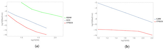
Figure 1. Efficiency curves of log maximum absolute error versus number of steps, NS. (a) Problem 1, (b) Problem 2.

In addition, we have solved the linear system in Problem 2 in order to compare the proposed ITPBO9 method with ISHD [5] of order nine and ILMM [6] of order six, which are presented in Table 3 and Table 4, respectively. In Table 3, we have considered the maximum absolute errors for step size $h=\frac{1}{2^j}$, $j=2,3,4,5$. While in Table 4, the numerical results have been obtained by considering the maximum absolute errors along the interval using a different number of steps where $NS$ refers to the number of steps. It can be observed that increasing the number of steps leads to a decrease in the error. Based on the efficiency curves in Figure 1 and Figure 2, the new ITPBO9 method is more efficient where it achieved a smaller maximum error compared to the other methods when the step size h decreases as well as when the number of steps taken is the same. Therefore, Table 3 and Table 4 and Figure 1 and Figure 2 clearly point out how ITPBO9 is superior in terms of accuracy and efficiency compared to the existing methods.

Table 3. Comparison of the maximum absolute errors on Problem 2, $t\in [0,2]$.

h	ISHD	ITPBO9
$1/4$	5.7164094 (−04)	6.169287 (−11)
$1/8$	4.8477800 (−08)	1.776357 (−14)
$1/16$	4.1669318 (−10)	3.552714 (−15)
$1/32$	3.4571600 (−12)	1.421085 (−15)

Table 4. Comparison of the maximum absolute errors on Problem 2, $t\in [0,2]$.

NS	ILMM	ITPBO9
10	5.446 (−03)	1.421085 (−12)
20	9.590 (−05)	9.521273 (−13)
40	1.804 (−06)	5.400125 (−13)
80	2.981 (−08)	3.126388 (−13)
160	5.291 (−10)	1.222134 (−14)

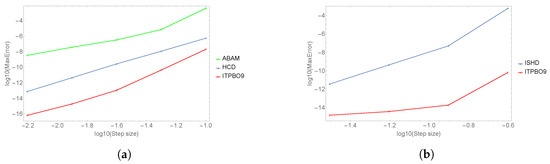
Figure 2. Efficiency curves of log maximum absolute error versus step size, h. (a) Problem 1, (b) Problem 2.

However, we have considered in Problem 3 and Problem 4 single and systems of nonlinear IVPs. Table 5, Table 6, Table 7 and Table 8 show the computed solutions compared to the exact solutions and the absolute errors at different points. It is remarkable that the computed solutions at each point t agree very well with the exact solutions up to 16 digits at least.

Table 5. Numerical findings for solving Problem 3, $h=0.01$.

t	Exact Solution	Computed Solution	AE (ITPBO9)
0.1	0.100167421161559790	0.100167421161559790	0.000000+00
$0.2$	0.201357920790330820	0.201357920790330770	5.551115 (−17)
$0.3$	0.304692654015397630	0.304692654015397520	1.110223 (−16)
$0.4$	0.411516846067488230	0.411516846067487900	3.330669 (−16)
$0.5$	0.523598775598299150	0.523598775598298700	4.440892 (−16)
$0.6$	0.643501108793284820	0.643501108793284370	4.440892 (−16)
$0.7$	0.775397496610753630	0.775397496610753080	5.551115 (−16)
$0.8$	0.927295218001613080	0.927295218001612190	8.881784 (−16)

Table 6. Numerical findings for solving $y_1$ of Problem 4, $h=0.01$, $t\in [0,1]$.

t	Exact Solution of ${\mathit{y}}_1$	Computed Solution of ${\mathit{y}}_1$	AE (ITPBO9) in ${\mathit{y}}_1$
$0.1$	0.904837418035959740	0.904837418035959630	0.000000+000
$0.3$	0.740818220681717880	0.740818220681717770	5.551115 (−17)
$0.5$	0.606530659712633310	0.606530659712633310	1.942890 (−16)
$0.7$	0.496585303791409300	0.496585303791409300	2.498002 (−16)
$0.9$	0.406569659740598940	0.406569659740598890	2.914335 (−16)

Table 7. Numerical findings for solving $y_2$ of Problem 4, $h=0.01$, $t\in [0,1]$.

t	Exact Solution of ${\mathit{y}}_2$	Computed Solution of ${\mathit{y}}_2$	AE (ITPBO9) in ${\mathit{y}}_2$
$0.1$	0.818730753077981710	0.818730753077981820	0.000000+000
$0.3$	0.548811636094026610	0.548811636094026280	5.551115 (−17)
$0.5$	0.367879441171442500	0.367879441171442170	1.942890 (−16)
$0.7$	0.246596963941606550	0.246596963941606270	2.498002 (−16)
$9.0$	0.165298888221586560	0.165298888221586340	2.914335 (−16)

Table 8. Numerical findings for solving $y_3$ of Problem 4, $h=0.01$, $t\in [0,1]$.

t	Exact Solution of ${\mathit{y}}_3$	Computed Solution of ${\mathit{y}}_3$	AE (ITPBO9) in ${\mathit{y}}_3$
$0.1$	0.740818220681717880	0.740818220681717880	0.000000+000
$0.3$	0.406569659740598890	0.406569659740598940	5.551115 (−17)
$0.5$	0.223130160148429480	0.223130160148429680	1.942890 (−16)
$0.7$	0.122456428252981490	0.122456428252981740	2.498002 (−16)
$0.9$	0.067205512739749340	0.067205512739749632	2.914335 (−16)

Overall, from all the tables and figures, the convergence and high precision of the new method is clearly observed. The method is more efficient than the existing methods, in which the order is either nearly equal or identical to that of the new method at each point t and each step size h.

5.2. Application to Thin Film Flow Problem

We also consider the well-known engineering and physical problem, which is the thin film flow of a liquid on a surface. This problem was studied by several authors [5,7,29,30,31]. They studied the fluid motion on a plane surface where the motion along the plane is in the same flow direction. The fluid dynamics problem is governed by the third-order ODEs

$$\begin{array}{c}\hfill y^{″}=f\left(y\left(t\right)\right),\end{array}$$

(24)

where $y\left(t\right)$ moves with the fluid in a coordinate frame and $f\left(y\right(t\left)\right)$ can vary depending on the physical context, such as

$$\begin{array}{c}\hfill f\left(y\left(t\right)\right)=y^{-2}-1\end{array}$$

(25)

is a formula for a fluid draining problem on a dry surface.

$$\begin{array}{c}\hfill f\left(y\left(t\right)\right)=(1+\xi +{\xi }^2)y^{-2}-(\xi +{\xi }^2)y^{-3}-1\end{array}$$

(26)

is a formula for a fluid draining problem on a wet surface where $\xi$ is the film thickness and $\xi >0$. Problems regarding the flow of thin films with a free surface of viscous fluid in which surface tension effects play a role commonly leads to third order ordinary ODEs governing the shape of the free surface of the fluid, which is given by

$$\begin{array}{c}\hfill y^{″}=y^{-\mu },t\ge t_0,\end{array}$$

(27)

subject to

$$y\left(t_0\right)=a_1,y^{\prime }\left(t_0\right)=a_2,y^{″}\left(t_0\right)=a_3,$$

where $a_1,a_2$ and $a_3$ are constants. In the literature, several researchers solve the problem (27) with the initial conditions $y\left(0\right)=y^{\prime }\left(0\right)=y^{″}\left(0\right)=1,$ for the case $\mu =2$. A parametric representation for the exact solution of (27) was introduced by [30].

For comparison purposes, we will apply the new method to solve (27) directly. The results are in Table 9 and Figure 3 clearly shows that the method is applicable and the solution that was obtained by ITPBO9 agrees very well with the exact solutions [30].

Table 9. Numerical findings for solving Problem (27) with $\mu =2$, $h=0.01$.

t	Exact Solution Ref. [30]	ISHD	ITPBO9	AE (ISHD)	AE (ITPBO9)
0.1	1.000000000	1.0000000000	1.0000000000	0.0000 + 000	0.0000 + 000
0.2	1.221211030	1.2212100137	1.2212100045	1.0163 (−06)	1.0255 (−06)
0.4	1.488834893	1.4888348170	1.4888347799	7.6000 (−08)	1.1310 (−07)
0.6	1.807361404	1.8073614815	1.8073613977	7.7500 (−08)	6.3000 (−09)
0.8	2.179819234	2.1797930619	2.1798192339	2.6172 (−05)	8.0000 (−11)
1.0	2.608275822	2.6082751000	2.6082748676	7.2200 (−07)	9.5440 (−07)

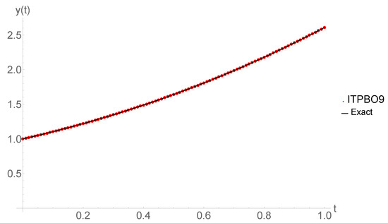
Figure 3. Response curve concerning Equation (27) with $\mu =2$, $h=0.01$.

5.3. Application to Boundary Layer Equation

A boundary layer in physics and fluid mechanics is the fluid layer in the immediate vicinity of a bounding surface in which the viscosity has significant effects. The equation of the nonlinear boundary layer is a nonlinear differential equation of third order defined as

$$\begin{array}{c}\hfill 2y^{″}+y{y}^{″}=0,\end{array}$$

(28)

subject to

$$\begin{array}{c}\hfill y\left(0\right)=y^{\prime }\left(0\right)=0,y^{″}\left(0\right)=1.\end{array}$$

It is a well known equation as the Blasius equation, which describes a boundary layer flow over a flat plate. This equation was already considered in [32,33]. We applied our method to solve the Blasius equation and to determine the shear stress at the plate. Figure 4 depicts that the solution to Equation (29) of the proposed method ITBPO9 in the interval $t\in [0,10]$ with $h=0.1$ agree very well with approximations found by the Mathematica built-in package NDSolve.

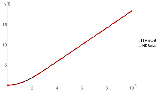
Figure 4. Response curve concerning Equation (29) with $h=0.1$ in $t\in [0,10]$.

5.4. Application to Nonlinear Genesio Equation

Consider the following nonlinear Genesio equation, which was introduced as a chaotic system by Genesio [34]

$$y^{″}+\alpha y^{″}+\beta y^{\prime }-f\left(y\left(t\right)\right)=0,$$

(29)

where

$$f(y\left(t\right)=-\gamma y\left(t\right)+y{\left(t\right)}^2,$$

subject to

$$y\left(t_0\right)=0.2,y^{\prime }\left(t_0\right)=-0.3,y^{″}\left(t_0\right)=0.1,t\in [0,b],$$

where $\alpha ,\beta$ and $\gamma$ are positive constants satisfying $\alpha \beta <\gamma$. The theoretical solution for this problem is unknown. This problem was studied by some researchers such as Bataineh et al. [35], which included the behavior of this system. Table 10 shows the computed solutions and the number of steps by the proposed ITPBO9 method, HCD [28] and the NDSolve at different b as well as different step sizes. We apply the new method to solve the nonlinear Genesio equation when $\alpha =1.2,\beta =2.92,\gamma =6$. It can be observed that ITPBO9 is applicable to solve Equation (29) with an advantage of fewer total steps compared to NDSolve. Figure 5 illustrates the numerical approximations for Equation (29) with $h=0.1$ in $t\in [0,4]$. It is obvious that the solutions obtained by ITPBO9 agree very well with approximations found by the Mathematica built-in package NDSolve that evaluate the efficiency of the new method.

Table 10. Numerical findings for solving Problem (29).

b	h	Method	Step	Computed Solution
$1.0$	0.1	ITPBO9	4	−0.0540040835391235
		HCD	4	−0.0540040832456468
		NDSolve	10	−0.0540040799051468
	0.01	ITPBO9	34	−0.0540040835547517
		HCD	34	−0.0540040835547393
		NDSolve	100	−0.0540040799051468
$4.0$	0.1	ITPBO9	13	−0.0676306051287455
		HCD	13	−0.0676305906240893
		NDSolve	40	−0.0676380593281975
	0.01	ITPBO9	133	−0.0676306051591404
		HCD	133	−0.0676306051590027
		NDSolve	400	−0.0676305976247482

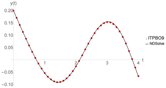
Figure 5. Response curve concerning Equation (29) with $h=0.1$ in $t\in [0,4]$.

6. Conclusions

In this article, we proposed a three-point implicit block method using the fourth and fifth derivatives of the solution, which aim to solve linear and nonlinear single as well as system initial value problems of the general third-order ODEs directly. The method is also applicable to solve the physical and engineering problems of the general third-order ODEs directly. The idea of incorporation of higher derivatives of the solution in the process, is that higher and better accuracy can be achieved without a corresponding increase in the order of the method. This new method is uncomplicated to implement and satisfies the property of convergence, which is indicated by the significant improvement with regards to accuracy in the numerical results. Therefore, we suggest the new ITPBO9 method as a suitable tool for solving general third-order ODEs directly with high precision and easy implementation.

References

- Boatto, S.; Kadanoff, L.P.; Olla, P. Traveling-wave solutions to thin-film equations. Phys. Rev. E 1993, 48, 4423. [Google Scholar] [CrossRef] [PubMed]
- Myers, T.G. Thin films with high surface tension. SIAM Rev. 1998, 40, 441–462. [Google Scholar] [CrossRef]
- Troy, W.C. Solutions of third-order differential equations relevant to draining and coating flows. SIAM J. Math. Anal. 1993, 24, 155–171. [Google Scholar] [CrossRef]
- Varlamov, V.V. The Third-Order Nonlinear Evolution Equation Governing Wave Propagation in Relaxing Media. Stud. Appl. Math. 1997, 99, 25–48. [Google Scholar] [CrossRef]
- Jikantoro, Y.; Ismail, F.; Senu, N.; Ibrahim, Z. A New Integrator for Special Third Order Differential Equations With Application to Thin Film Flow Problem. Indian J. Pure Appl. Math. 2018, 49, 151–167. [Google Scholar] [CrossRef]
- Jator, S.; Okunlola, T.; Biala, T.; Adeniyi, R. Direct Integrators for the General Third-Order Ordinary Differential Equations with an Application to the Korteweg–de Vries Equation. Int. J. Appl. Comput. Math. 2018, 4, 110. [Google Scholar] [CrossRef]
- Alkasassbeh, M.; Omar, Z. Hybrid one-step block fourth derivative method for the direct solution of third order initial value problems of ordinary differential equations. Int. J. Pure Appl. Math. 2018, 119, 207–224. [Google Scholar]
- Adeyeye, O.; Omar, Z. Direct solution of initial and boundary value problems of third order ODEs using maximal-order fourth-derivative block method. In AIP Conference Proceedings; AIP Publishing LLC: Melville, NY, USA, 2019; Volume 2138. [Google Scholar]
- Jeltsch, R.; Kratz, L. On the stability properties of Brown’s multistep multiderivative methods. Numer. Math. 1978, 30, 25–38. [Google Scholar] [CrossRef]
- Brugnano, L.; Trigiante, D. High-order multistep methods for boundary value problems. Appl. Numer. Math. 1995, 18, 79–94. [Google Scholar] [CrossRef]
- Awoyemi, D. A P-stable linear multistep method for solving general third order ordinary differential equations. Int. J. Comput. Math. 2003, 80, 985–991. [Google Scholar] [CrossRef]
- Majid, Z.A.; Suleiman, M.; Azmi, N.A. Variable step size block method for solving directly third order ordinary differential equations. Far East J. Math. Sci. 2010, 41, 63–73. [Google Scholar]
- Mechee, M.; Ismail, F.; Hussain, Z.M.; Siri, Z. Direct numerical methods for solving a class of third-order partial differential equations. Appl. Math. Comput. 2014, 247, 663–674. [Google Scholar] [CrossRef]
- Ramos, H.; Singh, G.; Kanwar, V.; Bhatia, S. An efficient variable step-size rational Falkner-type method for solving the special second-order IVP. Appl. Math. Comput. 2016, 291, 39–51. [Google Scholar] [CrossRef]
- Ramos, H.; Mehta, S.; Vigo-Aguiar, J. A unified approach for the development of k-step block Falkner-type methods for solving general second-order initial-value problems in ODEs. J. Comput. Appl. Math. 2017, 318, 550–564. [Google Scholar] [CrossRef]
- Jikantoro, Y.; Ismail, F.; Senu, N.; Ibrahim, Z.B. Hybrid methods for direct integration of special third order ordinary differential equations. Appl. Math. Comput. 2018, 320, 452–463. [Google Scholar] [CrossRef]
- Kuboye, J.; Omar, Z. Numerical solution of third order ordinary differential equations using a seven-step block method. Int. J. Math. Anal. 2014, 9, 743–754. [Google Scholar] [CrossRef]
- Awoyemi, D.; Kayode, S.; Adoghe, L. A five-step P-stable method for the numerical integration of third order ordinary differential equations. Am. J. Comput. Math. 2014, 4, 119–126. [Google Scholar] [CrossRef][Green Version]
- Ramos, H.; Rufai, M.A. Third derivative modification of k-step block Falkner methods for the numerical solution of second order initial-value problems. Appl. Math. Comput. 2018, 333, 231–245. [Google Scholar] [CrossRef]
- Ramos, H.; Rufai, M.A. A third-derivative two-step block Falkner-type method for solving general second-order boundary-value systems. Math. Comput. Simul. 2019, 165, 139–155. [Google Scholar] [CrossRef]
- Allogmany, R.; Ismail, F.; Ibrahim, Z.B. Implicit Two-point Block Method with Third and Fourth Derivatives for Solving General Second Order ODEs. Math. Stat. 2019, 7, 123. [Google Scholar] [CrossRef][Green Version]
- Wend, D.V. Existence and uniqueness of solutions of ordinary differential equations. Proc. Am. Math. Soc. 1969, 23, 27–33. [Google Scholar] [CrossRef]
- Wend, D. Uniqueness of solutions of ordinary differential equations. Am. Math. Mon. 1967, 74, 948–950. [Google Scholar] [CrossRef]
- Stoer, J.; Bulirsch, R. Introduction to Numerical Analysis; Springer: New York, NY, USA, 2002. [Google Scholar]
- Lambert, J.D. Numerical Methods for Ordinary Differential Systems: The Initial Value Problem; John Wiley & Sons, Inc.: New York, NY, USA, 1991. [Google Scholar]
- Fatunla, S.O. Numerical Methods for Initial Value Problems in Ordinary Differential Equations; Academic Press Inc.: New York, NY, USA, 1988. [Google Scholar]
- Ackleh, A.S.; Allen, E.J.; Kearfott, R.B.; Seshaiyer, P. Classical and Modern Numerical Analysis: Theory, Methods And Practice; Chapman and Hall/CRC: Boca Raton, FL, USA, 2009. [Google Scholar]
- Yap, L.K.; Ismail, F.; Senu, N. An accurate block hybrid collocation method for third order ordinary differential equations. J. Appl. Math. 2014, 2014. [Google Scholar] [CrossRef]
- Tuck, E.; Schwartz, L. A numerical and asymptotic study of some third-order ordinary differential equations relevant to draining and coating flows. SIAM Rev. 1990, 32, 453–469. [Google Scholar] [CrossRef]
- Duffy, B.; Wilson, S. A third-order differential equation arising in thin-film flows and relevant to Tanner’s law. Appl. Math. Lett. 1997, 10, 63–68. [Google Scholar] [CrossRef][Green Version]
- Mechee, M.; Senu, N.; Ismail, F.; Nikouravan, B.; Siri, Z. A three-stage fifth-order Runge-Kutta method for directly solving special third-order differential equation with application to thin film flow problem. Math. Probl. Eng. 2013, 2013, 795397. [Google Scholar] [CrossRef]
- Schlichting, H.; Gersten, K.; Krause, E.; Oertel, H.; Mayes, K. Boundary-Layer Theory; McGraw-Hill: New York, NY, USA, 1955. [Google Scholar]
- Lien-Tsai, Y.; Cha’o-Kuang, C. The solution of the Blasius equation by the differential transformation method. Math. Comput. Modell. 1998, 28, 101–111. [Google Scholar] [CrossRef]
- Genesio, R.; Tesi, A. Harmonic balance methods for the analysis of chaotic dynamics in nonlinear systems. Autom. J. IFAC 1992, 28, 531–548. [Google Scholar] [CrossRef]
- Bataineh, A.S.; Noorani, M.; Hashim, I. Direct Solution of n th-Order IVPs by Homotopy Analysis Method. Available online: https://projecteuclid.org/download/pdf_1/euclid.ijde/1485399721 (accessed on 5 March 2020).
© 2020 by the authors. Licensee MDPI, Basel, Switzerland. This article is an open access article distributed under the terms and conditions of the Creative Commons Attribution (CC BY) license (http://creativecommons.org/licenses/by/4.0/).