Further Properties of Quantum Spline Spaces

Abstract

We construct q-B-splines using a new form of truncated power functions. We give basic properties to show that q-B-splines form a basis for quantum spline spaces. On the other hand, we derive algorithmic formulas for $1/q$-integration and $1/q$-differentiation for q-spline functions. Moreover, we show a way to find the polynomial pieces on each interval of a q-spline function.

1. Introduction

B-splines were constructed by Lobachevsky as convolutions of certain probability distributions in the early 19th century. Spline functions are used in various numerical analysis areas like interpolation, approximation, computer aided geometric design, numerical solutions of differential equations, etc. The modern theory of spline approximation was started by Schoenberg in 1946, when he used B-splines for statistical data smoothing, see [1]. De Boor gave the recurrence relation for B-splines in [2]. Gordon and Reisenfield formally introduced B-splines into computer aided design in [3].

Mangasarian and Schumaker introduced discrete splines, h-splines, to solve discrete analogoues of minimization problems in a Banach space (see [4]). These discrete splines of degree n are defined on a subset of real line of the form ${[a,b]}_h=\{a,a+h,\dots ,a+Nh\}$, $b=a+Nh$, whose knot sequence is in $[a,b]$ and their polynomial pieces agree at the knots up to the order $n-1$ of forward differences with step size h instead of derivatives. In [5], q-splines which allow us to model tolerances, jumps and quantum leaps in the derivatives at the joins, were defined recursively based on a q-analogue of the de Boor algorithm. After giving certain properties, they defined blossoms for q-B-splines. In [6], fundamental formulas of classical B-splines were extended to q-B-splines. The q-splines are piecewise polynomials whose q-derivatives up to some order agree at the joins. A recent study relates q-B-splines with the q-Peano kernels of divided differences and solves a best approximation problem in the space of quantum integrable functions, see [7].

Let $t_0<t_1<\cdots <t_m$ be the knots, and let n be a nonnegative integer and $q\ne 0$ be a fixed real. A q-spline function of degree n having knots $t_0<t_1<\cdots <t_m$ is a function S such that

(i)

S is a polynomial of degree up to n on each interval $[t_{i-1},t_i)$, $i=1,2,\dots ,m$.

(ii)

S is quantum continuous of order $n-1$ at the knots.

Then, S is a continuous piecewise polynomial of degree at most n and quantum continuous of order $n-1$ at the knots. Here, “quantum continuous of order $n-1$ at the knots” means the quantum derivatives $D_{1/q}^k$, $k=0,\dots ,n-1$ of adjacent polynomial segments agree at the knots.

The rest of this paper is organized as follows. In Section 2, we begin with definitions and theorems in q-calculus concerning this work. In Section 3, we give some properties of q-B-splines and give proofs which are not stated explicitly in [5]. In Section 4, we find a new basis for the q-spline spaces with a given knot sequence and degree. We define q-B-splines in a different manner from [5,6] but similar to that of Curry and Schoenberg [8] in which the truncated power function played a significant role. Our approach is based on a certain q-truncated power function rather than the recursive definition of q-B-splines. We show how we can obtain quantum derivatives and quantum integrals of a given q-spline function. Furthermore, we find the polynomial pieces of a q-spline by using quantum derivatives.

2. Preliminaries

For a fixed parameter $q\ne 1$, the q-derivatives are defined by

$$\begin{array}{ccc}\hfill D_{q}f\left(t\right)& =& \frac{f\left(qt\right)-f\left(t\right)}{(q-1)t}\hfill \\ \hfill D_q^{n}f\left(t\right)& =& D_q\left(D_q^{n-1}f\left(t\right)\right),n⩾2.\hfill \end{array}$$

Indeed q-derivatives are approximations to classical derivatives and, if f is a differentiable function, then

$$\underset{q\to 1}{lim}{D}_{q}f\left(x\right)=Df\left(x\right).$$

For polynomials, it follows from the definition of the q-derivative that

$$D_q{x}^n={\left[n\right]}_q{x}^{n-1},$$

where the q-integers ${\left[n\right]}_q$ are defined by

$${\left[n\right]}_q=\left\{\begin{array}{cc}(1-q^n)/(1-q),\hfill & q\ne 1,\\ n,\hfill & q=1.\end{array}\right.$$

Furthermore, the q-factorial is defined by

$${\left[n\right]}_q!={\left[1\right]}_q\cdots {\left[n\right]}_q.$$

The next definition states the q-analogues of a classical definite integral; for details, one may see [9].

Definition 1.

Let $0<a<b$. Then, the definite q-integral of a function $f\left(x\right)$ is defined by a convergent series

$${\int }_0^{b}f\left(x\right)d_{q}x=(1-q)b\sum _{i=0}^{\infty }{q}^{i}f\left(q^{i}b\right)$$

and

$${\int }_a^{b}f\left(x\right)d_{q}x={\int }_0^{b}f\left(x\right)d_{q}x-{\int }_0^{a}f\left(x\right)d_{q}x.$$

Theorem 1.

If $F\left(x\right)$ is continuous at $x=0$, then

$${\int }_a^b{D}_{q}F\left(x\right)d_{q}x=F\left(b\right)-F\left(a\right)$$

where $0⩽a<b⩽\infty .$

3. Properties of $\mathbf{q}$-B-Splines

The q-B-splines are introduced first by Simeonov and Goldman in [5]. We give from [5,6] the important properties of q-B-splines that will be used in this work. Throughout the paper $N_{k,n}(t;q)$ refers to q-B-spline basis functions.

Property1. 

(Recurrence Relation) Let $n⩾1$ be an integer and $\{t_i;i=k,k+1,\dots ,k+n+1\}$ be a set of distinct real numbers. Then, q-B-splines satisfies the recurrence relation

$$N_{k,n}(t;q)={\displaystyle \frac{q^{n-1}t-t_k}{t_{k+n}-t_k}}{N}_{k,n-1}(t;q)+{\displaystyle \frac{t_{k+n+1}-q^{n-1}t}{t_{k+n+1}-t_{k+1}}}{N}_{k+1,n-1}(t;q)$$

(1)

with

$$N_{k,0}(t;q)=\left\{\begin{array}{cc}1,\hfill & t_k⩽t<t_{k+1}\hfill \\ 0,\hfill & \mathit{otherwise}.\hfill \end{array}\right.$$

Property 2.

$$N_{k,n}(t;q)=(t_{k+n+1}-t_k)[t_k,\dots ,t_{k+n+1}]{(x-t)}_{+}^{n,q},$$

(2)

where

$${(x-t)}_{+}^{n,q}=(x-q^{n-1}t)(x-q^{n-2}t)\cdots (x-qt){(x-t)}_{+}$$

and

$${(x-t)}_{+}=\left\{\begin{array}{cc}x-t,\hfill & \hfill \mathit{if}x⩾t\\ 0,\hfill & \hfill \mathit{if}x<t.\end{array}\right.$$

Property 3.

The interval of support of the q-B-spline: $support\left(N_{k,n}(t;q)\right)\subseteq [t_k,t_{k+n+1}]$.

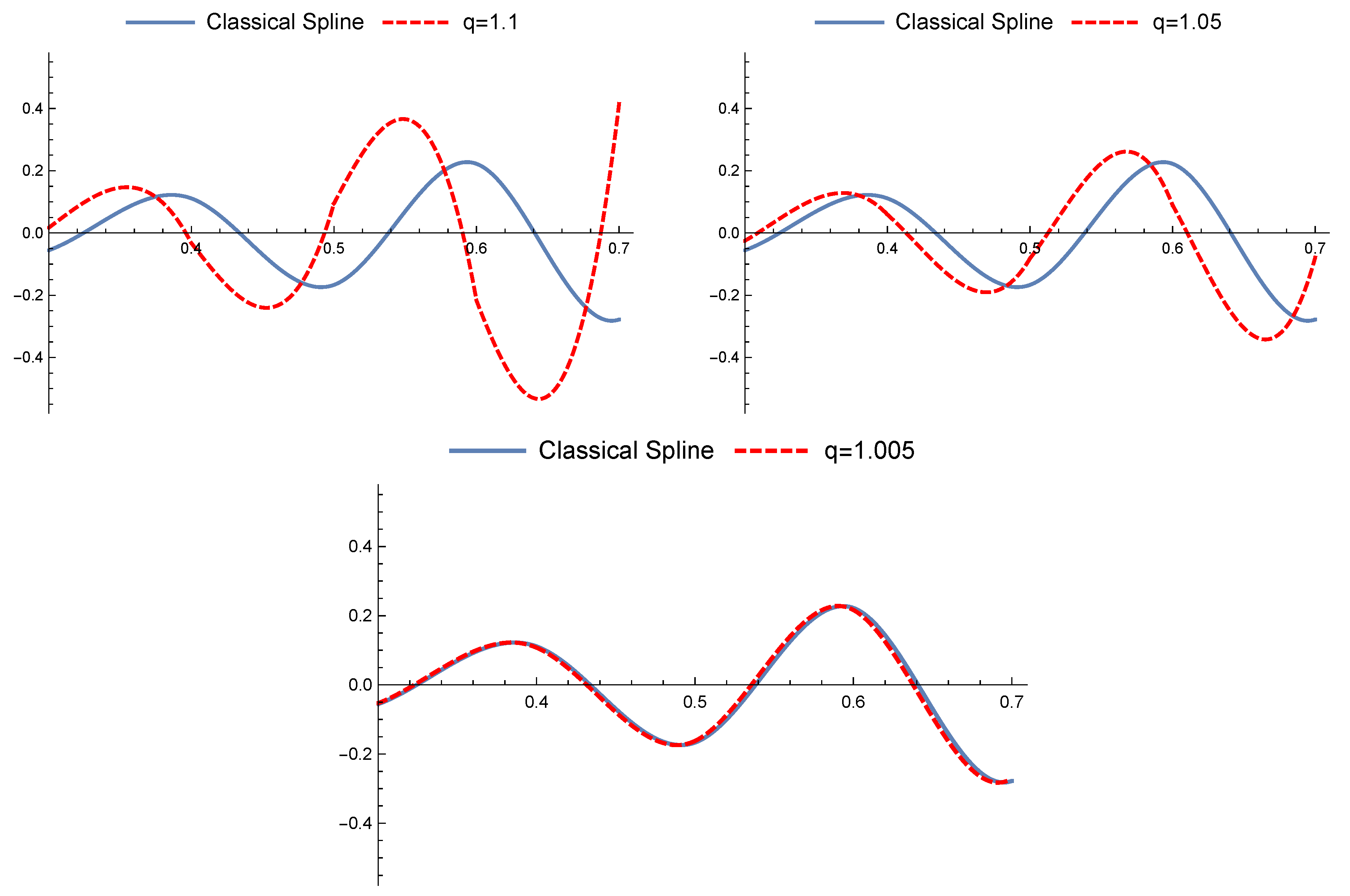
Property 4.

For any integer $n⩾2$, we have

$$D_{1/q}{N}_{k,n}(t;q)={\left[n\right]}_q\left(\frac{N_{k,n-1}(t;q)}{t_{k+n}-t_k}-\frac{N_{k+1,n-1}(t;q)}{t_{k+n+1}-t_{k+1}}\right).$$

(3)

Property 5.

Partition of unity:

$$\sum _k{N}_{k,n}(t;q)=1.$$

Remark 1.

The classical B-spline $N_{k,n}\left(t\right)$ is nonnegative for each k, n and all $t\in [t_k,t_{k+n+1}]$. However, Figure 1 shows that q-B-splines $N_{k,n}(t;q)$ may be nonnegative depending on the value of parameter q.

Figure 1. The graphs of $N_{0,2}(t;q)$ with the knot sequence $(1,2,3,4)$ and $q=2$, $q=1.5$, $q=1.1$ respectively, whose first order quantum derivatives agree at knots.

Remark 2.

If $q=1$, it is obvious that q-B-splines become classical B-splines and they mimic the classical counterpart when q is near 1.

Figure 2 compares q-B-spline curves with various values of q and for a fixed knot sequence and fixed control points.

Figure 2. q-B-spline curves with several q values, the knot sequence $\left\{0,\frac{1}{10},\frac{1}{5},\frac{3}{10},\frac{2}{5},\frac{1}{2},\frac{3}{5},\frac{7}{10},\frac{4}{5},\frac{9}{10},1\right\}$ and the control points $\left\{0,-\frac{1}{6},\frac{1}{3},-\frac{1}{2},\frac{2}{3},-\frac{5}{6},1\right\}$.

The following Lemmas 1, 2, and Proposition 1 are noted in [5]. Here, we prove them by using induction. We use the notation $N_{k,n}^q$ in the place of $N_{k,n}(t;q)$ to emphasize its dependence on the initial parameter value q.

Lemma 1.

For $n⩾1$, the q-B-splines $N_{k,n}^q$ belong to continuity class $q-C^{n-1}\left(\mathbb{R}\right)$ that is quantum derivatives of $N_{k,n}^q$ agree up to the order $n-1$ at the joins.

Proof. 

Since $N_{k,1}^q$ is continuous, we can say that $N_{k,1}^q\in q-C^0\left(\mathbb{R}\right).$ Suppose that $N_{k,n}^q\in q-C^{n-1}\left(\mathbb{R}\right)$. By Property 4, it follows that $D_{1/q}{N}_{k,n+1}^q\in q-C^{n-1}\left(\mathbb{R}\right)$. Thus, $N_{k,n+1}^q\in q-C^n\left(\mathbb{R}\right)$.  □

The following result shows that the sequence of q-B-splines of the same degree is linearly independent in a single interval of its support.

Lemma 2.

The set of q-B-splines $\{N_{i,n}^q,N_{i+1,n}^q,\dots ,N_{i+n,n}^q\}$ is linearly independent on $(t_{i+n},t_{i+n+1}).$

Proof. 

When $n=0$, it is obvious that the set is linearly independent. Let $n⩾1$ and assume that the Lemma 2 holds for $n-1$. Let $S={\displaystyle \sum _{k=0}^n}{c}_{i+k}{N}_{i+k,n}^q$ and suppose that the q-spline S restricted to the interval $(t_{i+n},t_{i+n+1})$, $S\left|\right(t_{i+n},t_{i+n+1})=0$. By Equation (3), we have

$$0=D_{1/q}S|(t_{i+n},t_{i+n+1})={\left[n\right]}_q\sum _{k=1}^n\left(\frac{c_{i+k}-c_{i+k-1}}{t_{i+k+n}-t_{i+k}}\right)N_{i+k,n-1}^q|(t_{i+n},t_{i+n+1}).$$

(4)

Since $N_{i+n+1,n-1}(t;q)=0$ and $N_{i,n-1}(t;q)=0$ on $(t_{i+n},t_{i+n+1})$, by induction hypothesis $\{N_{i+1,n-1}^q,\dots ,N_{i+n,n-1}^q\}$ is linearly independent on the interval $(t_{i+n},t_{i+n+1})$. Therefore, we must have that all the coefficients in Equation (4) are zero, that is, $c_i=c_{i+1}=\cdots =c_{i+n}$, say all of them equal to the value c. Thus, by the partition unity property of q-B-splines, we have $S(t;q)=c$ on $(t_{i+n},t_{i+n+1})$. Hence, by the assumption $S\left|\right(t_{i+n},t_{i+n+1})=0$, we have $c=0$ which shows that the set of q-B-splines $\{N_{i,n}^q,N_{i+1,n}^q,\dots ,N_{i+n,n}^q\}$ is linearly independent on an interval $(t_{i+n},t_{i+n+1}).$  □

Proposition 1.

The set of q-B-splines $\{N_{-n,n}^q,N_{-n+1,n}^q,\dots ,N_{m-1,n}^q\}$ is linearly independent on $(t_0,t_m).$

Proof. 

Let ${\displaystyle S=\sum _{k=-n}^{m-1}{c}_k{N}_{k,n}^q}$ and suppose $S\left|\right(t_0,t_m)=0$. For $0⩽i⩽m-1$, on the interval $(t_i,t_{i+1})$, only $\{N_{i-n,n}^q,N_{i-n+1,n}^q,\dots ,N_{i,n}^q\}$ are non-zero and we have

$$0=S|(t_i,t_{i+1})=\sum _{k=i-n}^i{c}_k{N}_{k,n}^q|(t_i,t_{i+1}).$$

(5)

From the previous lemma, the set $\{N_{i-n,n}^q,N_{i-n+1,n}^q,\dots ,N_{i,n}^q\}$ is linearly independent on $(t_i,t_{i+1})$. Hence, the coefficients $c_k=0$ for $i-n⩽k⩽i$ in Equation (5). If all the $c_k$’s are zero, then there is nothing to prove. Suppose, on the contrary, that not all the $c_k$’s are zero. Let j be the index such that $c_j\ne 0$. Assume $0⩽j⩽m-1$ and $(t_j,t_{j+1})\subset (t_0,t_m)$. For any $t\in (t_j,t_{j+1})$, we obtain

$$0=S(t;q)=\sum _{k=j}^{m-1}{c}_k{N}_{k,n}(t;q)=c_j{N}_{j,n}(t;q)\ne 0$$

which contradicts $S\left|\right(t_j,t_{j+1})=0$. Therefore, all the $c_k$’s are zero and this implies that the set $\{N_{-n,n}^q,N_{-n+1,n}^q,\dots ,N_{m-1,n}^q\}$ is linearly independent on $(t_0,t_m)$.  □

4. The Quantum Spline Space ${\mathcal{S}}_m^{n,q}$

Let ${\mathcal{S}}_m^{n,q}$ denote the space of the q-spline functions which are quantum continuous up to the order $n-1$, and n denotes the degree of polynomial pieces, $m+1$ is the number of knots in the knot sequence, and q is a nonzero initial parameter.

The next theorem shows that q-B-splines form a basis for the quantum spline space ${\mathcal{S}}_m^{n,q}$ of degree n with the knot sequence $t_0<t_1<\cdots <t_m$.

We note that, although the work [5] investigates broadly q-B-splines via blossoming, the following theorem and its proof were not mentioned.

Theorem 2.

A basis for the space ${\mathcal{S}}_m^{n,q}$ is

$$1,t,t^2,\dots ,t^n,{(t-t_1;q)}_{+}^n,{(t-t_2;q)}_{+}^n,\dots ,{(t-t_{m-1};q)}_{+}^n$$

where

$${(t-t_j;q)}_{+}^n=(q^{n-1}t-t_j)\cdots (qt-t_j){(t-t_j)}_{+}.$$

Consequently, the dimension of ${\mathcal{S}}_m^{n,q}$ is $n+m$ and q-B-splines $N_{i,n}^q|[t_0,t_m]$ with $-n⩽i⩽m-1$ form a basis for the q-spline space ${\mathcal{S}}_m^{n,q}$.

Proof. 

It is obvious that each $N_{i,n}^q|[t_0,t_m]$ for $-n⩽i⩽m-1$ is in the space ${\mathcal{S}}_m^{n,q}$. Thus, it is enough to show that the dimension of the space ${\mathcal{S}}_m^{n,q}$ is $m+n$. Firstly, we show that each element $S_m^n$ in ${\mathcal{S}}_m^{n,q}$ can be written in the form

$$S_m^n(t;q)=\sum _{i=0}^n{a}_i{t}^i+\sum _{i=1}^{m-1}{b}_i{(t-t_i;q)}_{+}^n.$$

(6)

Since in the interval $[t_0,t_1]$ all the truncated powers vanish, $S_m^n(t;q)$ is a polynomial of degree n, say ${\beta }_0$. Thus, we have $p_0(t;q)={\displaystyle \sum _{i=0}^n}{a}_i{t}^i$ which determines all the coefficients $a_i$. In the interval $[t_1,t_2]$, $S_m^n(t;q)$ is another polynomial, say ${\beta }_1$. According to the quantum continuity at the knots, we have at $t_1$,

$$D_{1/q}^r({\beta }_1-{\beta }_0)\left(t_1\right)=0,0⩽r⩽n-1.$$

Since ${\beta }_1-{\beta }_0$ is a polynomial of degree at most n, we have $({\beta }_1-{\beta }_0)(t;q)=b_1{(t-t_1;q)}^n$ for some $b_1$. Hence, we can write

$$S_m^n(t;q)=\sum _{i=0}^n{a}_i{t}^i+b_1{(t-t_1;q)}_{+}^n,t_0⩽t⩽t_2$$

When we repeat the same argument at the other internal knots $t_2,t_3,\dots ,t_{m-1}$, we obtain the q-spline in Equation (6). Thus, any spline of degree n on the interval $[t_0,t_m]$ with intermediate knots $t_1,t_2,\dots ,t_{m-1}$ may be written as a sum of multiples of $n+m$ functions

$$1,t,t^2,\dots ,t^n,{(t-t_1;q)}_{+}^n,{(t-t_2;q)}_{+}^n,\dots ,{(t-t_{m-1};q)}_{+}^n.$$

Since these functions are linearly independent, they form a basis for the this spline space and hence the dimension of the space ${\mathcal{S}}_m^{n,q}$ is $n+m$. Furthermore, it follows from Proposition 1 that q-B-splines $N_{i,n}^q|[t_0,t_m]$ with $-n⩽i⩽m-1$ form a basis for the space ${\mathcal{S}}_m^{n,q}$.  □

In [5], q-B-splines are constructed by using the de Boor algorithm. In the following theorem, we construct q-B-splines using properties of truncated power functions depending on q. Namely, we give explicit expression of q-B-spline basis functions in terms of linear combinations of q-truncated power functions.

Theorem 3.

$$N_{k,n}(t;q)={(-1)}^{n+1}(t_{k+n+1}-t_k)\sum _{j=k}^{k+n+1}\left[\prod _{\genfrac{}{}{0pt}{}{i=k}{i\ne j}}^{k+n+1}\frac{1}{(t_j-t_i)}\right]{(t-t_j;q)}_{+}^n$$

with respect to the normalization ${\sum }_k{N}_{k,n}(t;q)=1$.

Proof. 

Let $\{{\Psi }_j:j=1,2,\dots ,n+m\}$ be a basis in the expression

$$S(t;q)=\sum _{j=1}^{n+m}{\lambda }_j{\Psi }_j(t;q)a⩽t⩽b$$

such that each function $\{{\Psi }_j(t;q):j=1,2,\dots ,n+m\}$ is identically zero over a large part of the range $a⩽t⩽b$. Consider an element of the space $\mathcal{S}(n,t_0,\dots ,t_m)$ that is zero on the intervals $[t_0,t_k]$ and $[t_r,t_m]$, but that is nonzero on $(t_k,t_r)$, where $0<k<r<m$. If $\Phi$ is such a function, it can be expressed in the form

$$\Phi (t;q)=\sum _{j=k}^r{\mu }_j(q^{n-1}t-t_j)\cdots (qt-t_j){(t-t_j)}_{+},a⩽t⩽b$$

where the parameters ${\mu }_j$ have to satisfy the condition

$$\sum _{j=k}^r{\mu }_j(q^{n-1}t-t_j)\cdots (qt-t_j)(t-t_j)=0,t_r⩽t⩽b$$

since ${(t-t_j)}_{+}=0$ for $j=k,k+1,\dots ,r$ and $a⩽t⩽t_k$.

By rearranging the terms and using the properties of Lagrange polynomial interpolation, we have

$$\sum _{j=k}^r{\mu }_j{t}_j^i=0,i=0,1,\dots ,n.$$

(7)

If $r⩾k+n+1$, then equations in (7) have a nonzero solution. If $r=k+n+1$, then the coefficients are

$${\mu }_j=c\prod _{\genfrac{}{}{0pt}{}{i=k}{i\ne j}}^{k+n+1}\frac{1}{(t_i-t_j)},j=k,k+1,\dots ,k+n+1$$

where c is a nonzero constant. Thus, we can conclude that

$$\Phi (t;q)=\sum _{j=k}^{k+n+1}\left[c\prod _{\genfrac{}{}{0pt}{}{i=k}{i\ne j}}^{k+n+1}\frac{1}{(t_i-t_j)}\right]{(t-t_j;q)}_{+}^n.$$

By applying the normalization constraint ${\sum }_k{N}_{k,n}(t;q)=1$, we obtain the q-B-splines

$$N_{k,n}(t;q)={(-1)}^{n+1}(t_{k+n+1}-t_k)\sum _{j=k}^{k+n+1}\left[\prod _{\genfrac{}{}{0pt}{}{i=k}{i\ne j}}^{k+n+1}\frac{1}{(t_j-t_i)}\right]{(t-t_j;q)}_{+}^n.$$

(8)

 □

A consequence of the last expression is the following:

Corollary 1.

$$N_{k,n}(t;q)={(-1)}^{n+1}(t_{k+n+1}-t_k)[t_k,t_{k+1},\dots ,t_{k+n+1}]{(t-x;q)}_{+}^n$$

(9)

Proof. 

This follows from the following property of divided differences

$$[t_k,t_{k+1},\dots ,t_{k+n+1}]f=\sum _{j=k}^{k+n+1}f\left(t_j\right)\left[\prod _{\genfrac{}{}{0pt}{}{i=k}{i\ne j}}^{k+n+1}\frac{1}{(t_j-t_i)}\right]$$

by replacing f by the truncated power function.  □

Remark 3.

One can easily show that q-B-spline basis functions defined in Equation (2) (Theorem 6 in [6]) are right continuous and that the q-B-spline basis functions defined in Equation (9) are left continuous.

We have shown that q-B-splines form a basis for q-splines. Now, let us investigate how we can find the quantum derivatives $D_{1/q}^j$ of the q-spline functions. The following algorithms allow us to store, evaluate, and manipulate q-splines on a computer easily, see [10]. In addition, we show that $1/q$-derivatives of q-splines are again q-spline functions.

Theorem 4.

Let S be a given q-spline function such that ${\displaystyle S(t;q)=\sum _{i=-n}^k{a}_i{N}_{i,n}(t;q)}$. Then, for all $j\in \{1,2,\dots ,n-1\}$ and all $t\in [a,b]$

$$D_{1/q}^{j}S(t;q)=\sum _{i=-n+j}^k{a}_i^{\left(j\right)}{N}_{i,n-j}(t;q),$$

(10)

where

$$a_i^{\left(j\right)}=\left\{\begin{array}{cc}{a}_i,\hfill & \mathit{if}j=0\hfill \\ {[n+1-j]}_q{\displaystyle \frac{a_i^{(j-1)}-a_{i-1}^{(j-1)}}{t_{i+n+1-j}-t_i}},\hfill & \mathit{if}j>0.\hfill \end{array}\right.$$

(11)

Proof. 

For $j=1$, we have

$$\begin{array}{ccc}\hfill D_{1/q}S(t;q)& =& \sum _{i=-n}^k{a}_i{D}_{1/q}{N}_{i,n}(t;q)\hfill \\ & =& \sum _{i=-n}^k{a}_i{\left[n\right]}_q\left(\frac{N_{i,n-1}(t;q)}{t_{i+n}-t_i}-\frac{N_{i+1,n-1}(t;q)}{t_{i+n+1}-t_{i+1}}\right)\hfill \\ & =& \sum _{i=-n}^k{\left[n\right]}_q\left(\frac{a_i}{t_{i+n}-t_i}{N}_{i,n-1}(t;q)-\frac{a_i}{t_{i+n+1}-t_{i+1}}{N}_{i+1,n-1}(t;q)\right)\hfill \\ & =& \sum _{i=-n+1}^k{\left[n\right]}_q\left(\frac{a_i-a_{i-1}}{t_{i+n}-t_i}\right)N_{i,n-1}(t;q).\hfill \end{array}$$

This shows that Equation (11) is true for $j=1$. Repeating the same argument shows that the formula (11) is true for each $j=1,2,\dots ,n-1.$  □

Now, we derive a formula for computing the $1/q$-integral of a given q-spline function.

Theorem 5.

Let S be a given q-spline function such that ${\displaystyle S(t;q)=\sum _{i=-n}^k{a}_i{N}_{i,n}(t;q)}$. Then, for all $t\in [a,b]$,

$${\int }_{t_{-n}}^{t}S(x;q)d_{1/q}x=\sum _{i=-n}^k\left(\sum _{j=-n}^i{a}_j\frac{t_{j+m+1}-t_j}{{[n+1]}_q}\right)N_{i,n+1}(t;q).$$

(12)

Proof. 

Define a function $\tilde{S}$ by

$$\tilde{S}(t;q)={\int }_{t_{-n}}^{t}S(x;q)d_{1/q}x.$$

This is a quantum spline of degree $n+1$ and so $\tilde{S}$ can be written as

$$\tilde{S}(t;q)=\sum _{i=-n}^k{\tilde{a}}_i{N}_{i,n+1}(t;q).$$

Using (10) and (11) for all $t\in [a,b]$ gives

$$S(t;q)=D_{1/q}\tilde{S}(t;q)=\sum _{i=-n}^k{[n+1]}_q\frac{{\tilde{a}}_i-{\tilde{a}}_{i-1}}{t_{i+n+1}-t_i}{N}_{i,n}(t;q),$$

where ${\tilde{a}}_{-m-1}=0.$ It follows by comparing the appropriate coefficients of the basis that

$$a_i=\frac{{[n+1]}_q}{t_{i+n+1}-t_i}{\tilde{a}}_i\mathrm{for}i=-n$$

and

$$a_i=\frac{{[n+1]}_q}{t_{i+n+1}-t_i}\left({\tilde{a}}_i-{\tilde{a}}_{i-1}\right)\mathrm{for}i=-n+1,\dots ,k.$$

Therefore,

$${\tilde{a}}_i=\sum _{j=-n}^i{a}_j\frac{t_{j+m+1}-t_j}{{[n+1]}_q}\mathrm{for}i=-n,-n+1,\dots ,k$$

and this completes the proof.  □

In the next proposition, we demonstrate a way to find the polynomials on each interval of a q-spline function. In certain circumstances, we may have to evaluate the q-spline function S at a large number of points, then it is advantageous to determine the polynomial pieces at each interval $P_j{(t;q)=S|}_{[t_j,t_{j+1})}$ for each j.

Proposition 2.

Let $S(t;q)$ be a q-spline function such that

$$S(t;q)=\sum _{i=-n}^k{a}_i{N}_{i,n}(t;q),t\in [a,b]$$

and $P_j$ be the polynomial restricted to ${S|}_{[t_j,t_{j+1})}$ for $j=0,\dots ,k.$ Then,

$$P_j(t;q)=\sum _{r=0}^n\frac{1}{{\left[r\right]}_q!}\left(D_{1/q}^{r}S(t_j;q)\right)(q^{r-1}t-t_j)\cdots (qt-t_j)(t-t_j),t\in [t_j,t_{j+1})$$

Proof. 

Since $S(t;q)$ is a polynomial of degree n on the interval $[t_j,t_{j+1})$ for each $j=0,1,\dots ,k$, we can write

$$P_j(t;q)=\sum _{r=0}^n{\lambda }_{rj}{(t-t_j;q)}^r,$$

where ${\lambda }_{rj}$ for $r=0,1,\dots ,n$ and $j=0,1,\dots ,k$ are the unknowns and

$${(t-t_j;q)}^r=(q^{r-1}t-t_j)\cdots (qt-t_j)(t-t_j).$$

Then, it is easily seen that, by taking $1/q$-derivative of $S(t;q)$r times, substituting $t=t_j$ in Equation (10) gives

$${\lambda }_{rj}=\frac{1}{{\left[r\right]}_q!}{D}_{1/q}^{r}S(t_j;q).$$

Hence, we obtain

$$P_j(t;q)=\sum _{r=0}^n\frac{1}{{\left[r\right]}_q!}{D}_{1/q}^{r}S(t_j;q){(t-t_j;q)}^r,t\in [t_j,t_{j+1}).$$

 □

5. Conclusions

In this work, we derived a new way to compute q-B-spline $N_{k,n}(t;q)$ and algorithms for q-derivatives and q-integrals of a q-spline function, and found the polynomial pieces on a specified single interval. These formulas will be useful in numerical methods incorporating a finite difference scheme with q-B-splines. For CAGD purposes, we take the parameter values q near 1 in q-B-spline curves so as to mimic the behavior of their classical counterpart. Besides solving a best approximation problem, not only q-B-splines but also h-splines share certain fundamental properties of the classical B-splines. In a future work, we will study how we can solve partial q-differential equations by using q-splines. We will introduce box q-splines as well as their rational counterpart and then investigate them in solving certain PDE problems towards isogeometric analysis.