A Modified Self-Adaptive Conjugate Gradient Method for Solving Convex Constrained Monotone Nonlinear Equations for Signal Recovery Problems

Abstract

In this article, we propose a modified self-adaptive conjugate gradient algorithm for handling nonlinear monotone equations with the constraints being convex. Under some nice conditions, the global convergence of the method was established. Numerical examples reported show that the method is promising and efficient for solving monotone nonlinear equations. In addition, we applied the proposed algorithm to solve sparse signal reconstruction problems.

1. Introduction

Suppose $\Omega$ is a nonempty, closed and convex subset of $R^n$, F a continuous function from $R^n$ to $R^n$. A constrained nonlinear monotone equation involves finding a point $x\in \Omega$, such that

$$F\left(x\right)=0.$$

(1)

Many algorithms have been proposed in the literature to solve nonlinear constrained equations, some of which are the trust region and the Levenberg-Marquardt method [1]. However, the need for these methods to compute and store matrix in every iteration, make them unsuitable for solving large-scale nonlinear equations.

Conjugate gradient (CG) methods is an iterative method developed for handling the unconstrained optimization problem [2,3,4,5,6,7,8,9]. CG methods do not require matrix storage, which make them one of the most efficient methods for handling large-scale unconstrained optimization problems. Moreover, generating a descent direction does not always hold based on the secant conditions. In order to obtain a descent direction, Narushima et al. [6] and Zhang et al. [8] proposed three term CG methods, which always generate a descent direction and established the convergence of the methods under some suitable conditions. Also in Reference [5], Narushima proposed a smoothing CG algorithm, which combine the smoothing approach with the Polak–Ribière–Polyak CG methods in Reference [9], to handle unconstrained non-smooth equations. The convergence of the method was established under some mild conditions.

Methods for solving unconstrained problems sometimes become less useful (see for example References [10,11,12,13]), as in many practical applications, such as equilibrium problems, the solution of the unconstrained problem may lie outside the constrained set $\Omega$. This reason made researchers shift their attention to the constrained case (1). In the last few years, many kinds of algorithms for solving nonlinear monotone equations with convex constrained set $\Omega$ have been developed and one of the popular is the projection method. For example, in Reference [14] Wang et al. proposed a projection method for solving systems of monotone nonlinear equations with convex constraints. The method was based on the inexact Newton backtracking technique and the direction was obtained by minimization of a linear system together with the constrained condition at each iteration. Also, in Reference [15] Wang et al. presented a modification of the method in Reference [16], and the global convergence as well as the super-linear rate of convergence were established under same conditions in Reference [14]. However, the direction of the methods in Reference [15,16] were determined by minimization of linear equations at each step. In trying to avoid solving the linear equation to obtain the direction at each step, Xiao and Zhu [17] proposed a projected CG methods, which combines the CG-DESCENT method in [4] and the projection technique by Solodov and Svaiter [18]. In Reference [19], a modification of the method in Reference [17] was proposed by Liu and Li. The advantage of this modification was that it improves the numerical performance of the method in Reference [17] and still retains its nice properties. Furthermore, Wang et al. [20] proposed a self-adaptive three-term CG methods for solving constrained nonlinear monotone equations. The method can be viewed as combination of the CG methods, the projection method and the self-adaptive method. Motivated by the above methods, we propose a modification of the method in Reference [20] for solving nonlinear monotone equations with convex constraints. The modification improves the numerical performance of the method in Reference [20] and still inherits its nice properties. The difference between the two methods is that $y_{k-1}$ in Reference [20] is replaced by $w_{k-1}$ (More details can be found in the next section). Under appropriate conditions, the global convergence of the proposed method is established. Numerical results presented show that the proposed method is efficient and promising compared to some similar existing algorithms.

The remaining part of this paper is organized as follows. In Section 2, we state some preliminaries and then present the algorithm. The global convergence of the proposed method is proved in Section 3. In Section 4, we report some numerical experiments to show its performance in solving nonlinear monotone equations with convex constraints, and lastly apply it to solve some signal recovery problems.

2. Preliminaries and Algorithm

This section gives some basic concepts and properties of the projection mapping as well as some assumptions. $\parallel ·\parallel$ denotes the Euclidean norm throughout the paper.

Definition 1.

Let $\Omega \subset R^n$ be a nonempty closed convex set. Then for any $x\in R^n$, its orthogonal projection onto Ω, denoted by $P_{\Omega }\left(x\right)$, is defined by

$$P_{\Omega }\left(x\right)=argmin\{\parallel x-y\parallel :y\in \Omega \}.$$

The following Lemma provides us with some well-known properties of the projection mapping.

Lemma 1.

[20] Let $\Omega \subset R^n$ be a nonempty, closed and convex set. Then the following statements are true:

1. 

${(x-P_{\Omega }\left(x\right))}^T(P_{\Omega }\left(x\right)-z)\ge 0$, $\forall x\in R^n,z\in \Omega .$

2. 

$\parallel P_{\Omega }\left(x\right)-P_{\Omega }\left(y\right)\parallel \le \parallel x-y\parallel$, $\forall x,y\in R^n.$

3. 

$\parallel P_{\Omega }{\left(x\right)-z\parallel }^2\le {\parallel x-z\parallel }^2-{\parallel x-P_{\Omega }\left(x\right)\parallel }^2$, $\forall x\in R^n,z\in \Omega .$

All through this article, we assume the following

($A_1$) 

The solution set of (1), denoted by ${\Omega }^{{}^{\prime }}$, is nonempty.

($A_2$) 

The mapping F is monotone, that is,

$${(F\left(x\right)-F\left(y\right))}^T(x-y)\ge 0,\forall x,y\in R^n.$$

($A_3$) 

The mapping $F(.)$ is Lipschitz continuous, that is there exists a positive constant L such that $\parallel F\left(x\right)-F\left(y\right)\parallel \le L\parallel x-y\parallel$, $\forall x,y\in R^n$.

Algorithm 1: Modified Self-adaptive CG method (MSCG).
	Step 0. Given an arbitrary initial point $x_0\in \Omega$, parameters $\beta >0$, $r>0$, $0<\mu <2$, $\sigma >0$, $0<\rho <1$, $Tol>0$, and set $k:=0$.
	Step 1.  If $\parallel F\left(x_k\right)\parallel \le Tol$, stop, otherwise go to Step 2.
	Step 2.  Compute $$d_k=\left\{\begin{array}{cc}-F\left(x_k\right),\hfill & \mathrm{if}k=0,\hfill \\ -F\left(x_k\right)+{\beta }_k^{{}^{\prime }}{d}_{k-1}-{\theta }_k^{{}^{\prime }}{w}_{k-1},\hfill & \mathrm{if}k\ge 1,\hfill \end{array}\right.$$ (2) where $${\beta }_k^{{}^{\prime }}=\frac{F{\left(x_k\right)}^T{w}_{k-1}}{d_{k-1}^T{w}_{k-1}},{\theta }_k^{{}^{\prime }}=\frac{F{\left(x_k\right)}^T{d}_{k-1}}{d_{k-1}^T{w}_{k-1}}$$ (3) $$y_{k-1}=F\left(x_k\right)-F\left(x_{k-1}\right)+r{s}_{k-1},s_{k-1}=x_k-x_{k-1},$$ (4) $$w_{k-1}=y_{k-1}+t_{k-1}{d}_{k-1},t_{k-1}=1+max\left\{0,-\frac{d_{k-1}^T{y}_{k-1}}{d_{k-1}^T{d}_{k-1}}\right\}.$$ (5)
	Step 3.  Compute the step length ${\alpha }_k=\beta {\rho }^{m_k}$ and $m_k$ is the smallest non-negative integer m such that $$-⟨F(x_k+\beta {\rho }^m{d}_k),d_k⟩\ge \sigma \beta {\rho }^m{\parallel d_k\parallel }^2.$$ (6)
	Step 4.  Set $z_k=x_k+{\alpha }_k{d}_k$ and compute $$x_{k+1}=P_{\Omega }[x_k-\mu {\zeta }_{k}F\left(z_k\right)]$$ where $${\zeta }_k=\frac{F{\left(z_k\right)}^T(x_k-z_k)}{\parallel F\left(z_k\right){\parallel }^2}.$$
	Step 5.  Let $k=k+1$ and go to Step 1.

It can be observed that the modification made is by replacing ${\beta }_k^{HS}$, ${\theta }_k$ in [20] with ${\beta }_k^{{}^{\prime }}$, ${\theta }_k^{{}^{\prime }}$ respectively in the proposed algorithm.

Remark 1.

$$\begin{array}{cc}\hfill {F(x}_k{)}^T{d}_k& =-F{\left(x_k\right)}^{T}F\left(x_k\right)+\frac{F{\left(x_k\right)}^T\left(F{\left(x_k\right)}^T{w}_{k-1}\right)d_{k-1}-F{\left(x_k\right)}^T\left(F{\left(x_k\right)}^T{d}_{k-1}\right)w_{k-1}}{d_{k-1}^T{w}_{k-1}}\hfill \\ & =-\parallel F\left(x_k\right){\parallel }^2+\frac{\left(F{\left(x_k\right)}^T{d}_{k-1}\right)\left(F{\left(x_k\right)}^T{w}_{k-1}\right)-\left(F{\left(x_k\right)}^T{w}_{k-1}\right)\left(F{\left(x_k\right)}^T{d}_{k-1}\right)}{d_{k-1}^T{w}_{k-1}}\hfill \\ & =-\parallel F\left(x_k\right){\parallel }^2.\hfill \end{array}$$

(7)

Using Cauchy-Schwartz inequality, we get

$$\parallel F\left(x_k\right)\parallel \le \parallel d_k\parallel .$$

(8)

Remark 2.

From the definition of $w_{k-1}$, $t_{k-1}$ and (8), we have

$$d_{k-1}^T{w}_{k-1}\ge d_{k-1}^T{y}_{k-1}+\parallel d_{k-1}{\parallel }^2-d_{k-1}^T{y}_{k-1}={\parallel d_{k-1}\parallel }^2$$

(9)

The above inequality shows that the denominator of ${\beta }_k^{{}^{\prime }}$ and ${\theta }_k^{{}^{\prime }}$ cannot be zero except at the solution. However, there is no any guarantee that the denominator of ${\beta }_k^{HS}$ and ${\theta }_k$ defined in Reference [20] cannot be zero. In addition, the conditions imposed in step 2 of Algorithm 2.1 of [20] were not considered in our case.

3. Convergence Analysis

To prove the global convergence of Algorithm 1, the following Lemmas are needed. The following Lemma shows that Algorithm 1 is well-defined.

Lemma 2.

Suppose that assumptions ($A_1$)–($A_3$) hold, then there exists a step-length ${\alpha }_k$ satisfying the line search (6) $\forall k\ge 0$.

Proof. 

Suppose there exists $k_0\ge 0$ such that (6) does not hold for any non-negative integer i, that is,

$$-⟨F(x_{k_0}+\beta {\rho }^i{d}_{k_0}),d_{k_0}⟩<\sigma \beta {\rho }^i{\parallel d_{k_0}\parallel }^2.$$

Using assumption ($A_3$) and allowing $i\to \infty$, we get

$$-⟨F\left(x_{k_0}\right),d_{k_0}⟩\le 0.$$

(10)

Also from (7), we have

$$-⟨F\left(x_{k_0}\right),d_{k_0}⟩={\parallel F\left(x_{k_0}\right)\parallel }^2>0,$$

which contradicts (10). The proof is complete. □

Lemma 3.

Suppose that ($A_3$) hold and the sequences $\left\{x_k\right\}$ and $\left\{z_k\right\}$ be generated by Algorithm 1. Then we have

$${\alpha }_k\ge \rho min\left\{\beta ,\rho \frac{\parallel F\left(x_k\right){\parallel }^2}{(L+\sigma )\parallel d_k{\parallel }^2}\right\}.$$

Proof. 

Suppose ${\alpha }_k\ne \beta$, then $\frac{{\alpha }_k}{\rho }$ does not satisfy Equation (6), that is

$$-F{\left(x_k+\frac{{\alpha }_k}{\rho }{d}_k\right)}^T{d}_k<\sigma \frac{{\alpha }_k}{\rho }{\parallel d_k\parallel }^2.$$

This combined with (7) and the fact that F is Lipschitz continuous yields

$$\begin{array}{cc}\hfill \parallel F\left(x_k\right){\parallel }^2& =-F{\left(x_k\right)}^T{d}_k\hfill \\ & ={\left(F(x_k+\frac{{\alpha }_k}{\rho }{d}_k)-F\left(x_k\right)\right)}^T{d}_k-F{\left(x_k+\frac{{\alpha }_k}{\rho }{d}_k\right)}^T{d}_k\hfill \\ & \le L\frac{{\alpha }_k}{\rho }\parallel d_k{\parallel }^2+\sigma \frac{{\alpha }_k}{\rho }{\parallel d_k\parallel }^2\hfill \\ & =\frac{L+\sigma }{\rho }{\alpha }_k{\parallel d_k\parallel }^2.\hfill \end{array}$$

(11)

The above equation implies

$${\alpha }_k\ge \rho \frac{\parallel F\left(x_k\right){\parallel }^2}{(L+\sigma )\parallel d_k{\parallel }^2},$$

which completes the proof. □

Lemma 4.

Suppose that assumptions ($A_1$)–($A_3$) hold, then the sequences $\left\{x_k\right\}$ and $\left\{z_k\right\}$ generated by Algorithm 1 are bounded. Moreover, we have

$$\underset{k\to \infty }{lim}\parallel x_k-z_k\parallel =0,$$

(12)

and

$$\underset{k\to \infty }{lim}\parallel x_{k+1}-x_k\parallel =0.$$

(13)

Proof. 

We will start by showing that the sequences $\left\{x_k\right\}$ and $\left\{z_k\right\}$ are bounded. Suppose $\overline{x}\in {\Omega }^{{}^{\prime }}$, then by monotonicity of F, we get

$$⟨F\left(z_k\right),x_k-\overline{x}⟩\ge ⟨F\left(z_k\right),x_k-z_k⟩.$$

(14)

Also by definition of $z_k$ and the line search (6), we have

$$⟨F\left(z_k\right),x_k-z_k⟩\ge \sigma {\alpha }_k^2{\parallel d_k\parallel }^2\ge 0.$$

(15)

So, we have

$$\begin{array}{cc}\hfill \parallel x_{k+1}-\overline{x}{\parallel }^2& =\parallel P_{\Omega }[x_k-\mu {\zeta }_{k}F\left(z_k\right)]-\overline{x}{\parallel }^2\hfill \\ & \le \parallel x_k-\mu {\zeta }_{k}F\left(z_k\right)-\overline{x}{\parallel }^2\hfill \\ & =\parallel x_k-\overline{x}{\parallel }^2-2\mu {\zeta }_k⟨F\left(z_k\right),x_k-\overline{x}⟩+{\parallel \mu {\zeta }_{k}F\left(z_k\right)\parallel }^2\hfill \\ & =\parallel x_k-\overline{x}{\parallel }^2-2\mu \frac{⟨F\left(z_k\right),x_k-z_k⟩}{\parallel F\left(z_k\right){\parallel }^2}⟨F\left(z_k\right),x_k-\overline{x}⟩+{\mu }^2{\left(\frac{⟨F\left(z_k\right),x_k-z_k⟩}{\parallel F\left(z_k\right)\parallel }\right)}^2\hfill \\ & \le \parallel x_k-\overline{x}{\parallel }^2-2\mu \frac{⟨F\left(z_k\right),x_k-z_k⟩}{\parallel F\left(z_k\right){\parallel }^2}⟨F\left(z_k\right),x_k-z_k⟩+{\mu }^2{\left(\frac{⟨F\left(z_k\right),x_k-z_k⟩}{\parallel F\left(z_k\right)\parallel }\right)}^2\hfill \\ & \le \parallel x_k-\overline{x}{\parallel }^2-\mu (2-\mu ){\left(\frac{⟨F\left(z_k\right),x_k-z_k⟩}{\parallel F\left(z_k\right)\parallel }\right)}^2\hfill \\ & =\parallel x_k-\overline{x}{\parallel }^2-\mu (2-\mu )\frac{{\sigma }^2{\parallel x_k-z_k\parallel }^4}{\parallel F\left(z_k\right){\parallel }^2}.\hfill \end{array}$$

(16)

Thus the sequence $\{\parallel x_k-\overline{x}\parallel \}$ is non increasing and convergent and hence $\left\{x_k\right\}$ is bounded. Furthermore, from Equation (16), we have

$$\parallel x_{k+1}-\overline{x}{\parallel }^2\le {\parallel x_k-\overline{x}\parallel }^2,$$

(17)

and we can deduce recursively that

$$\parallel x_k-\overline{x}{\parallel }^2\le {\parallel x_0-\overline{x}\parallel }^2,\forall k\ge 0.$$

Then from Assumption ($A_3$), we obtain

$$\parallel F\left(x_k\right)\parallel =\parallel F\left(x_k\right)-F\left(\overline{x}\right)\parallel \le L\parallel x_k-\overline{x}\parallel \le L\parallel x_0-\overline{x}\parallel .$$

If we let $L\parallel x_0-\overline{x}\parallel =\omega$, then the sequence $\left\{F\left(x_k\right)\right\}$ is bounded, that is,

$$\parallel F\left(x_k\right)\parallel \le \omega ,\forall k\ge 0.$$

(18)

By the definition of $z_k$, Equation (15), monotonicity of F and the Cauchy-Schwatz inequality, we get

$$\sigma \parallel x_k-z_k\parallel =\frac{\sigma \parallel {\alpha }_k{d}_k{\parallel }^2}{\parallel x_k-z_k\parallel }\le \frac{⟨F\left(z_k\right),x_k-z_k⟩}{\parallel x_k-z_k\parallel }\le \frac{⟨F\left(x_k\right),x_k-z_k⟩}{\parallel x_k-z_k\parallel }\le \parallel F\left(x_k\right)\parallel .$$

(19)

The boundedness of the sequence $\left\{x_k\right\}$ together with Equations (18) and (19), implies that the sequence $\left\{z_k\right\}$ is bounded.

Since $\left\{z_k\right\}$ is bounded, then for any $\overline{x}\in {\Omega }^{{}^{\prime }}$, the sequence $\{z_k-\overline{x}\}$ is also bounded, that is, there exists a positive constant $\nu >0$ such that

$$\parallel z_k-\overline{x}\parallel \le \nu ,\forall k\ge 0.$$

This together with Assumption ($A_3$) yields

$$\parallel F\left(z_k\right)\parallel =\parallel F\left(z_k\right)-F\left(\overline{x}\right)\parallel \le L\parallel z_k-\overline{x}\parallel \le L\nu .$$

Therefore, using Equation (16), we have

$$\mu (2-\mu )\frac{{\sigma }^2}{{\left(L\nu \right)}^2}\parallel x_k-z_k{\parallel }^4\le \parallel x_k-\overline{x}{\parallel }^2-{\parallel x_{k+1}-\overline{x}\parallel }^2,$$

which implies

$$\mu (2-\mu )\frac{{\sigma }^2}{{\left(L\nu \right)}^2}\sum _{k=0}^{\infty }\parallel x_k-z_k{\parallel }^4\le \sum _{k=0}^{\infty }(\parallel x_k-\overline{x}{\parallel }^2-\parallel x_{k+1}-\overline{x}{\parallel }^2)\le \parallel x_0-\overline{x}\parallel <\infty .$$

(20)

Equation (20) implies

$$\underset{k\to \infty }{lim}\parallel x_k-z_k\parallel =0.$$

However, using statement 2 of Lemma 1, the definition of ${\zeta }_k$ and the Cauchy-Schwatz inequality, we have

$$\begin{array}{cc}\hfill \parallel x_{k+1}-x_k\parallel & =\parallel P_{\Omega }[x_k-\mu {\zeta }_{k}F\left(z_k\right)]-x_k\parallel \hfill \\ & =\parallel x_k-\mu {\zeta }_{k}F\left(z_k\right)-x_k\parallel \hfill \\ & =\parallel \mu {\zeta }_{k}F\left(z_k\right)\parallel \hfill \\ & =\mu \parallel x_k-z_k\parallel ,\forall k\ge 0,\hfill \end{array}$$

(21)

which yields

$$\underset{k\to \infty }{lim}\parallel x_{k+1}-x_k\parallel =0.$$

 □

Remark 3.

By Equation (12) and definition of $z_k$, we have

$$\underset{k\to \infty }{lim}{\alpha }_k\parallel d_k\parallel =0.$$

(22)

Theorem 1.

Suppose that assumptions ($A_1$)–($A_3$) hold and let the sequence $\left\{x_k\right\}$ be generated by Algorithm 1, then

$${\displaystyle \underset{k\to \infty }{lim\; inf}\parallel F\left(x_k\right)\parallel =0.}$$

(23)

Proof. 

Assume that Equation (23) is not true, then there exists a constant $ϵ>0$ such that

$$\parallel F\left(x_k\right)\parallel \ge ϵ,\forall k\ge 0.$$

(24)

We will first show that the sequence $\left\{d_k\right\}$ is bounded. From the definition of $t_{k-1}$, we have

$$\begin{array}{cc}\hfill |t_{k-1}|& =\left|1+max\left\{0,-\frac{d_{k-1}^T{y}_{k-1}}{\parallel d_{k-1}{\parallel }^2}\right\}\right|\hfill \\ & \le 1+\frac{|d_{k-1}^T{y}_{k-1}|}{\parallel d_{k-1}{\parallel }^2}\hfill \\ & \le 1+\frac{\parallel d_{k-1}\parallel \parallel y_{k-1}\parallel }{\parallel d_{k-1}{\parallel }^2}\hfill \\ & =1+\frac{\parallel y_{k-1}\parallel }{\parallel d_{k-1}\parallel }.\hfill \end{array}$$

(25)

Also from definition of $y_{k-1}$ and assumption ($A_3$), we have

$$\begin{array}{cc}\hfill \parallel y_{k-1}\parallel & \le \parallel F\left(x_k\right)-F\left(x_{k-1}\right)\parallel +r\parallel s_{k-1}\parallel \hfill \\ & \le (L+r)\parallel s_{k-1}\parallel \hfill \\ & \le (L+r){\alpha }_{k-1}\parallel d_{k-1}\parallel .\hfill \end{array}$$

(26)

Furthermore by definition of $w_{k-1}$, (25) and (26), we obtain

$$\begin{array}{cc}\hfill \parallel w_{k-1}\parallel & =\parallel y_{k-1}+t_{k-1}{d}_{k-1}\parallel \hfill \\ & \le \parallel y_{k-1}\parallel +|t_{k-1}|\parallel d_{k-1}\parallel \hfill \\ & \le (L+r){\alpha }_{k-1}\parallel d_{k-1}\parallel +\left(1+\frac{\parallel y_{k-1}\parallel }{\parallel d_{k-1}\parallel }\right)\parallel d_{k-1}\parallel \hfill \\ & =(L+r){\alpha }_{k-1}\parallel d_{k-1}\parallel +\parallel d_{k-1}\parallel +\parallel y_{k-1}\parallel \hfill \\ & \le (2(L+r){\alpha }_{k-1}+1)\parallel d_{k-1}\parallel .\hfill \end{array}$$

(27)

Therefore, by (2), (9), (18), (27) and Cauchy-Schwatz inequality, we have

$$\begin{array}{cc}\hfill \parallel d_k\parallel & \le \parallel F\left(x_k\right)\parallel +\frac{\parallel F\left(x_k\right)\parallel \parallel w_{k-1}\parallel \parallel d_{k-1}\parallel }{|d_{k-1}^T{w}_{k-1}|}+\frac{\parallel F\left(x_k\right)\parallel \parallel d_{k-1}\parallel \parallel w_{k-1}\parallel }{|d_{k-1}^T{w}_{k-1}|}\hfill \\ & \le \parallel F\left(x_k\right)\parallel +(4(L+r){\alpha }_{k-1}+2)\parallel F\left(x_k\right)\parallel \hfill \\ & =(1+4(L+r){\alpha }_{k-1}+2)\parallel F\left(x_k\right)\parallel \hfill \\ & \le (1+4(L+r)\beta +2)\omega .\hfill \end{array}$$

(28)

Letting $C=(1+4(L+r)\beta +2)\omega$, then $\parallel d_k\parallel \le C,\forall k\ge 0.$

Combining (8) and (24), we have

$$\parallel d_k\parallel \ge \parallel F\left(x_k\right)\parallel \ge ϵ,\forall k\ge 0.$$

As $z_k=x_k+{\alpha }_k{d}_k$ and ${lim}_{k\to \infty }\parallel x_k-z_k\parallel =0$, we get ${lim}_{k\to \infty }{\alpha }_k\parallel d_k\parallel =0$ and

$$\underset{k\to \infty }{lim}{\alpha }_k=0.$$

(29)

On the other side, Lemma 3 and (28) imply ${\alpha }_k\parallel d_k\parallel \ge min\left\{\beta ϵ\frac{{ϵ}^2}{(L+\sigma )C^2}\right\}$, which contradicts with (29). Therefore, (23) must hold. □

4. Numerical Examples

This section reports some numerical results to show the efficiency of Algorithm 1. For convenience sake, we denote Algorithm 1 by the modified self-adaptive method MSCG. We also divide this section into two. First we compare the MSCG method with the projected conjugate gradient PCG and the self-adaptive three-term conjugate gradient SATCGM methods in References [19,20] respectively, by solving some monotone nonlinear equations with convex constraints using different initial points and several dimensions. Secondly, the MSCG method is applied to solve signal recovery problems. All codes were written in MATLAB R2017a and run on a PC with intel COREi5 processor with 4 GB of RAM and CPU 2.3 GHZ.

4.1. Numerical Examples on Some Convex Constrained Nonlinear Monotone Equations

Same line search implementation was used for both MSCG, PCG and SATCGM. The specific parameters used for each method are as follows:

MSCG method:

$\beta =1$, $\mu =1.8$, $\rho =0.6$, $r=0.1$, $\sigma =0.0001$.

PCG method:

All parameters are chosen as in [19].

SATCGM method:

All parameters are chosen as in [20]. All runs were stopped whenever $\parallel F\left(x_k\right)\parallel <{10}^{-6}.$

We test problems 1 to 9 with dimensions of n = 1000, 5000, 10,000, 50,000, 100,000 and different initial points: $x_1={(1,1,\dots ,1)}^T$, $x_2={(2,2,\dots ,2)}^T$, $x_3={(3,3,\dots ,3)}^T$, $x_4={(5,5,\dots ,5)}^T$, $x_5={(8,8,\dots ,8)}^T$, $x_6={(0.5,0.5,\dots 0.5)}^T$, $x_7={(0.1,0.1,\dots ,0.1)}^T$, $x_8={(10,10,\dots ,10)}^T$. The numerical results in Table 1, Table 2, Table 3, Table 4, Table 5, Table 6, Table 7, Table 8 and Table 9 report the number of iterations (Iter), number of function evaluations (Fval), CPU time in seconds (Time) and the norm at the approximate solution (Norm). The symbol ‘−’ is used to indicate that the number of iterations exceeds 1000 and/or the number of function evaluations exceeds 2000.

Table 1. Numerical Results for modified self-adaptive method MSCG, projected conjugate gradient PCG and the self-adaptive three-term conjugate gradient SATCGM for Problem 1 with given initial points and dimensions.

		MSCG				PCG				SATCGM
Dimension	Initial Point	Iter	Fval	Time	Norm	Iter	Fval	Time	Norm	Iter	Fval	Time	Norm
1000	$x_1$	2	9	0.007489	0	52	189	0.110321	8.55$\times {10}^{-7}$	0	1	0.000488	0
	$x_2$	2	10	0.005551	0	56	204	0.035141	8.99$\times {10}^{-7}$	2	9	0.001201	0
	$x_3$	2	11	0.014899	0	56	205	0.033533	8.39$\times {10}^{-7}$	2	10	0.000999	0
	$x_3$	2	14	0.006243	0	65	237	0.041638	8.27$\times {10}^{-7}$	8	39	0.002423	7.2$\times {10}^{-7}$
	$x_5$	2	19	0.006022	0	78	310	0.05362	9.48$\times {10}^{-7}$	2	16	0.001369	0
	$x_6$	2	9	0.002681	0	54	196	0.035021	6.83$\times {10}^{-7}$	7	29	0.001878	2.24$\times {10}^{-7}$
	$x_7$	2	9	0.004044	0	49	178	0.042635	7.85$\times {10}^{-7}$	2	8	0.001429	0
	$x_8$	2	23	0.005336	0	69	266	0.043962	8.44$\times {10}^{-7}$	9	48	0.002906	1.14$\times {10}^{-7}$
5000	$x_1$	2	9	0.022857	0	50	183	0.09149	9.98$\times {10}^{-7}$	0	1	0.000807	0
	$x_2$	2	10	0.006854	0	56	205	0.103092	6.81$\times {10}^{-7}$	26	132	0.050119	5.8$\times {10}^{-7}$
	$x_3$	2	11	0.011049	0	54	199	0.104065	9.9$\times {10}^{-7}$	27	137	0.053248	6.74$\times {10}^{-7}$
	$x_3$	2	14	0.011355	0	64	234	0.115013	9.48$\times {10}^{-7}$	26	134	0.058245	9.79$\times {10}^{-7}$
	$x_5$	2	19	0.013144	0	70	278	0.131778	8.96$\times {10}^{-7}$	2	16	0.007147	0
	$x_6$	2	9	0.012189	0	53	193	0.09886	7.86$\times {10}^{-7}$	24	120	0.04757	9.33$\times {10}^{-7}$
	$x_7$	2	9	0.009516	0	47	172	0.095304	9.24$\times {10}^{-7}$	21	106	0.046785	9.89$\times {10}^{-7}$
	$x_8$	2	23	0.014401	0	70	269	0.128741	6.8$\times {10}^{-7}$	26	141	0.052327	8.83$\times {10}^{-7}$
10,000	$x_1$	2	9	0.017626	0	51	187	0.173696	6.85$\times {10}^{-7}$	0	1	0.001096	0
	$x_2$	2	10	0.013878	0	55	202	0.242626	7.46$\times {10}^{-7}$	25	127	0.101565	9.68$\times {10}^{-7}$
	$x_3$	2	11	0.016471	0	55	203	0.181091	6.79$\times {10}^{-7}$	27	137	0.101702	6.74$\times {10}^{-7}$
	$x_3$	2	14	0.016887	0	64	234	0.207939	9.63$\times {10}^{-7}$	26	134	0.086415	9.78$\times {10}^{-7}$
	$x_5$	2	19	0.019661	0	87	467	0.370102	9.32$\times {10}^{-7}$	2	16	0.012166	0
	$x_6$	2	9	0.011591	0	52	190	0.166351	8.5$\times {10}^{-7}$	24	120	0.078086	9.33$\times {10}^{-7}$
	$x_7$	2	9	0.011988	0	46	169	0.15083	1$\times {10}^{-6}$	21	106	0.072047	9.43$\times {10}^{-7}$
	$x_8$	2	23	0.022006	0	68	262	0.215882	9.85$\times {10}^{-7}$	26	141	0.100132	8.39$\times {10}^{-7}$
50,000	$x_1$	2	9	0.040326	0	49	181	0.707163	8.25$\times {10}^{-7}$	0	1	0.003271	0
	$x_2$	2	10	0.039481	0	54	199	0.901824	8.74$\times {10}^{-7}$	25	127	0.408502	8.76$\times {10}^{-7}$
	$x_3$	2	11	0.044192	0	53	197	0.779749	8.21$\times {10}^{-7}$	27	137	0.431524	6.74$\times {10}^{-7}$
	$x_3$	2	14	0.066019	0	63	232	1.047125	7.61$\times {10}^{-7}$	26	134	0.432464	9.78$\times {10}^{-7}$
	$x_5$	2	19	0.062454	0	73	293	1.479499	7.54$\times {10}^{-7}$	2	16	0.055519	0
	$x_6$	2	9	0.038738	0	51	187	0.769376	9.74$\times {10}^{-7}$	24	120	0.359623	9.32$\times {10}^{-7}$
	$x_7$	2	9	0.048211	0	46	170	0.650199	7.66$\times {10}^{-7}$	21	106	0.340155	8.53$\times {10}^{-7}$
	$x_8$	2	23	0.075239	0	68	262	1.034824	9.43$\times {10}^{-7}$	26	141	0.427085	7.54$\times {10}^{-7}$
100,000	$x_1$	2	9	0.071954	0	49	181	1.456718	8.7$\times {10}^{-7}$	0	1	0.005325	0
	$x_2$	2	10	0.070337	0	53	196	1.564101	9.51$\times {10}^{-7}$	25	127	0.795299	8.39$\times {10}^{-7}$
	$x_3$	2	11	0.129537	0	53	197	1.632904	8.69$\times {10}^{-7}$	27	137	0.805937	6.74$\times {10}^{-7}$
	$x_3$	2	14	0.103765	0	62	229	1.858922	8.28$\times {10}^{-7}$	26	134	0.816302	9.78$\times {10}^{-7}$
	$x_5$	2	19	0.132033	0	91	394	2.909579	9.4$\times {10}^{-7}$	2	16	0.104851	0
	$x_6$	2	9	0.066613	0	51	188	1.480664	7.13$\times {10}^{-7}$	24	120	0.708975	9.32$\times {10}^{-7}$
	$x_7$	2	9	0.070007	0	46	170	1.334943	8.04$\times {10}^{-7}$	21	106	0.623866	8.17$\times {10}^{-7}$
	$x_8$	2	23	0.158984	0	68	262	1.981132	9.39$\times {10}^{-7}$	26	141	0.841829	7.23$\times {10}^{-7}$

Table 2. Numerical Results for MSCG, PCG and SATCGM for Problem 2 with given initial points and dimensions.

		MSCG				PCG				SATCGM
Dimension	Initial Point	Iter	Fval	Time	Norm	Iter	Fval	Time	Norm	Iter	Fval	Time	Norm
1000	$x_1$	2	7	0.002287	0	4	9	0.005149	0	0	1	0.041011	0
	$x_2$	3	10	0.002837	0	5	11	0.005127	0	14	43	0.006989	1.84$\times {10}^{-7}$
	$x_3$	3	10	0.0042	0	6	13	0.004934	0	378	1135	0.221475	0
	$x_3$	3	10	0.004002	0	7	15	0.006266	0	373	1120	0.078963	0
	$x_5$	4	13	0.004927	0	9	19	0.009583	0	371	1114	0.071626	0
	$x_6$	2	7	0.002839	0	3	7	0.003695	0	8	25	0.00237	7.06$\times {10}^{-7}$
	$x_7$	2	7	0.003192	0	2	5	0.003077	0	7	22	0.002122	1.55$\times {10}^{-7}$
	$x_8$	5	16	0.005398	0	10	21	0.008973	0	371	1114	0.077539	0
5000	$x_1$	2	7	0.005581	0	4	9	0.009838	0	0	1	0.000878	0
	$x_2$	3	10	0.012182	0	5	11	0.012215	0	9	36	0.020012	1.86$\times {10}^{-7}$
	$x_3$	3	10	0.014385	0	6	13	0.016737	0	3	10	0.005862	0
	$x_3$	3	10	0.009594	0	7	15	0.017589	0	3	10	0.007543	0
	$x_5$	4	13	0.011344	0	9	19	0.020153	0	4	13	0.008266	0
	$x_6$	2	7	0.007545	0	3	7	0.010968	0	2	7	0.004719	0
	$x_7$	2	7	0.006425	0	2	5	0.008253	0	9	37	0.019936	1.09$\times {10}^{-7}$
	$x_8$	5	16	0.018064	0	10	21	0.024443	0	12	46	0.024472	1.72$\times {10}^{-7}$
10,000	$x_1$	2	7	0.01418	0	4	9	0.018819	0	0	1	0.001023	0
	$x_2$	3	10	0.014155	0	5	11	0.021572	0	9	36	0.032795	2.56$\times {10}^{-7}$
	$x_3$	3	10	0.014925	0	6	13	0.024532	0	3	10	0.010619	0
	$x_3$	3	10	0.014886	0	7	15	0.028731	0	3	10	0.010295	0
	$x_5$	4	13	0.017717	0	9	19	0.033857	0	4	13	0.015479	0
	$x_6$	2	7	0.010365	0	3	7	0.018178	0	2	7	0.006803	0
	$x_7$	2	7	0.010509	0	2	5	0.012152	0	9	37	0.033013	1.53$\times {10}^{-7}$
	$x_8$	5	16	0.022966	0	10	21	0.037341	0	12	46	0.042546	2.37$\times {10}^{-7}$
50,000	$x_1$	2	7	0.032816	0	4	9	0.059874	0	0	1	0.003458	0
	$x_2$	3	10	0.057053	0	5	11	0.080753	0	9	36	0.137308	5.63$\times {10}^{-7}$
	$x_3$	3	10	0.047544	0	6	13	0.088801	0	3	10	0.044405	0
	$x_3$	3	10	0.045036	0	7	15	0.102315	0	3	10	0.039837	0
	$x_5$	4	13	0.063642	0	9	19	0.129467	0	4	13	0.057216	0
	$x_6$	2	7	0.034852	0	3	7	0.054439	0	2	7	0.030166	0
	$x_7$	2	7	0.035797	0	2	5	0.035327	0	9	37	0.132406	3.41$\times {10}^{-7}$
	$x_8$	5	16	0.087191	0	10	21	0.143865	0	12	46	0.189329	5.22$\times {10}^{-7}$
100,000	$x_1$	2	7	0.057021	0	4	9	0.119186	0	0	1	0.005345	0
	$x_2$	3	10	0.091601	0	5	11	0.144375	0	9	36	0.290364	7.94$\times {10}^{-7}$
	$x_3$	3	10	0.0876	0	6	13	0.176278	0	3	10	0.081386	0
	$x_3$	3	10	0.11867	0	7	15	0.202121	0	3	10	0.078766	0
	$x_5$	4	13	0.122207	0	9	19	0.254424	0	4	13	0.105536	0
	$x_6$	2	7	0.061273	0	3	7	0.092884	0	2	7	0.050801	0
	$x_7$	2	7	0.086732	0	2	5	0.064906	0	9	37	0.30913	4.82$\times {10}^{-7}$
	$x_8$	5	16	0.137848	0	10	21	0.279527	0	12	46	0.384466	7.36$\times {10}^{-7}$

Table 3. Numerical Results for MSCG, PCG and SATCGM for Problem 3 with given initial points and dimensions.

		MSCG				PCG				SATCGM
Dimension	Initial Point	Iter	Fval	Time	Norm	Iter	Fval	Time	Norm	Iter	Fval	Time	Norm
1000	$x_1$	2	8	0.002131	0	11	29	0.007647	5.91$\times {10}^{-7}$	0	1	0.030317	0
	$x_2$	2	8	0.002618	0	11	29	0.006415	9.95$\times {10}^{-7}$	2	8	0.003362	0
	$x_3$	2	9	0.003474	0	11	30	0.007009	7.4$\times {10}^{-7}$	8	34	0.003058	4.12$\times {10}^{-7}$
	$x_3$	2	9	0.003267	0	13	36	0.010125	5.86$\times {10}^{-7}$	7	30	0.002381	9.62$\times {10}^{-7}$
	$x_5$	2	9	0.002792	0	12	34	0.006802	1.45$\times {10}^{-7}$	3	13	0.001892	0
	$x_6$	2	8	0.003134	0	11	29	0.008319	6.19$\times {10}^{-7}$	7	29	0.002217	4.45$\times {10}^{-7}$
	$x_7$	2	8	0.00293	0	10	26	0.008698	3.51E-07	7	29	0.002266	1.39$\times {10}^{-7}$
	$x_8$	2	9	0.003217	0	12	34	0.011399	1.02$\times {10}^{-7}$	8	34	0.002792	1.8$\times {10}^{-7}$
5000	$x_1$	2	8	0.004982	0	12	31	0.023695	1.23$\times {10}^{-7}$	0	1	0.000694	0
	$x_2$	2	8	0.007135	0	12	32	0.024907	9.71$\times {10}^{-7}$	2	8	0.004892	0
	$x_3$	2	9	0.009629	0	12	33	0.024784	7.22$\times {10}^{-7}$	10	42	0.018214	2.06$\times {10}^{-7}$
	$x_3$	2	9	0.009662	0	14	38	0.028132	1.22$\times {10}^{-7}$	9	38	0.017115	4.81$\times {10}^{-7}$
	$x_5$	2	9	0.007819	0	12	34	0.025162	3.25$\times {10}^{-7}$	3	13	0.00673	0
	$x_6$	2	8	0.006236	0	12	31	0.022688	1.28$\times {10}^{-7}$	9	37	0.01618	2.22$\times {10}^{-7}$
	$x_7$	2	8	0.00624	0	10	26	0.019349	7.85$\times {10}^{-7}$	8	33	0.014479	6.96$\times {10}^{-7}$
	$x_8$	2	9	0.006238	0	12	34	0.026113	2.27$\times {10}^{-7}$	9	38	0.018184	9$\times {10}^{-7}$
10,000	$x_1$	2	8	0.008726	0	12	31	0.042552	1.73$\times {10}^{-7}$	0	1	0.001391	0
	$x_2$	2	8	0.012242	0	13	34	0.04396	1.27$\times {10}^{-7}$	2	8	0.007936	0
	$x_3$	2	9	0.012729	0	13	35	0.041531	9.47$\times {10}^{-7}$	10	42	0.032685	2.92$\times {10}^{-7}$
	$x_3$	2	9	0.012833	0	14	38	0.043616	1.72$\times {10}^{-7}$	9	38	0.02903	6.8$\times {10}^{-7}$
	$x_5$	2	9	0.008266	0	12	34	0.040575	4.59$\times {10}^{-7}$	3	13	0.011808	0
	$x_6$	2	8	0.018599	0	12	31	0.037381	1.81$\times {10}^{-7}$	9	37	0.027841	3.14$\times {10}^{-7}$
	$x_7$	2	8	0.009012	0	11	29	0.034501	4.84$\times {10}^{-7}$	8	33	0.025044	9.85$\times {10}^{-7}$
	$x_8$	2	9	0.009328	0	12	34	0.042223	3.21$\times {10}^{-7}$	10	42	0.031896	1.27$\times {10}^{-7}$
50,000	$x_1$	2	8	0.032446	0	12	31	0.139558	3.88$\times {10}^{-7}$	0	1	0.003099	0
	$x_2$	2	8	0.04508	0	13	34	0.153158	2.85$\times {10}^{-7}$	2	8	0.026479	0
	$x_3$	2	9	0.035499	0	13	35	0.154392	2.12$\times {10}^{-7}$	10	42	0.144432	6.52$\times {10}^{-7}$
	$x_3$	2	9	0.043984	0	14	38	0.165244	3.85$\times {10}^{-7}$	10	42	0.135136	1.52$\times {10}^{-7}$
	$x_5$	2	9	0.037903	0	13	37	0.162555	4.48$\times {10}^{-7}$	3	13	0.043419	0
	$x_6$	2	8	0.03081	0	12	31	0.135904	4.06$\times {10}^{-7}$	9	37	0.114776	7.03$\times {10}^{-7}$
	$x_7$	2	8	0.031101	0	12	31	0.133471	1.01$\times {10}^{-7}$	9	37	0.114557	2.2$\times {10}^{-7}$
	$x_8$	2	9	0.034806	0	12	34	0.148058	7.18$\times {10}^{-7}$	10	42	0.156754	2.85$\times {10}^{-7}$
100,000	$x_1$	2	8	0.063409	0	12	31	0.272996	5.48$\times {10}^{-7}$	0	1	0.004848	0
	$x_2$	2	8	0.064054	0	13	34	0.298372	4.03$\times {10}^{-7}$	2	8	0.051739	0
	$x_3$	2	9	0.085457	0	13	35	0.303707	2.99$\times {10}^{-7}$	10	42	0.246669	9.22$\times {10}^{-7}$
	$x_3$	2	9	0.065247	0	14	38	0.329149	5.44$\times {10}^{-7}$	10	42	0.253435	2.15$\times {10}^{-7}$
	$x_5$	2	9	0.070299	0	13	37	0.324363	6.34$\times {10}^{-7}$	3	13	0.083962	0
	$x_6$	2	8	0.058418	0	12	31	0.272816	5.74$\times {10}^{-7}$	9	37	0.221264	9.94$\times {10}^{-7}$
	$x_7$	2	8	0.056572	0	12	31	0.274954	1.42$\times {10}^{-7}$	9	37	0.223174	3.11$\times {10}^{-7}$
	$x_8$	2	9	0.092306	0	13	37	0.357351	4.43$\times {10}^{-7}$	10	42	0.254061	4.03$\times {10}^{-7}$

Table 4. Numerical Results for MSCG, PCG and SATCGM for Problem 4 with given initial points and dimensions.

		MSCG				PCG				SATCGM
Dimension	Initial Point	Iter	Fval	Time	Norm	Iter	Fval	Time	Norm	Iter	Fval	Time	Norm
1000	$x_1$	2	8	0.002519	0	-	-	-	-	0	1	0.032812	0
	$x_2$	2	8	0.004286	0	-	-	-	-	655	1967	0.139812	9.97$\times {10}^{-7}$
	$x_3$	2	8	0.003714	0	-	-	-	-	655	1967	0.124618	9.98$\times {10}^{-7}$
	$x_3$	2	8	0.004556	0	-	-	-	-	649	1949	0.126132	9.98$\times {10}^{-7}$
	$x_5$	2	8	0.005003	0	-	-	-	-	656	1971	0.129295	9.98$\times {10}^{-7}$
	$x_6$	-	-	-	-	-	-	-	-	648	1945	0.12381	9.98$\times {10}^{-7}$
	$x_7$	-	-	-	-	-	-	-	-	652	1957	0.132922	9.98$\times {10}^{-7}$
	$x_8$	2	8	0.002868	0	-	-	-	-	654	1965	0.12119	9.98$\times {10}^{-7}$
5000	$x_1$	2	8	0.012432	0	-	-	-	-	0	1	0.001131	0
	$x_2$	2	8	0.011534	0	-	-	-	-	-	-	-	-
	$x_3$	2	8	0.009014	0	-	-	-	-	-	-	-	-
	$x_3$	2	8	0.008944	0	-	-	-	-	-	-	-	-
	$x_5$	2	8	0.009143	0	-	-	-	-	-	-	-	-
	$x_6$	-	-	-	-	-	-	-	-	-	-	-	-
	$x_7$	-	-	-	-	-	-	-	-	-	-	-	-
	$x_8$	2	8	0.010586	0	-	-	-	-	-	-	-	-
10,000	$x_1$	2	8	0.013601	0	-	-	-	-	0	1	0.00148	0
	$x_2$	2	8	0.017482	0	-	-	-	-	-	-	-	-
	$x_3$	2	8	0.020485	0	-	-	-	-	-	-	-	-
	$x_3$	2	8	0.016717	0	-	-	-	-	-	-	-	-
	$x_5$	2	8	0.016828	0	-	-	-	-	-	-	-	-
	$x_6$	-	-	-	-	-	-	-	-	-	-	-	-
	$x_7$	-	-	-	-	-	-	-	-	-	-	-	-
	$x_8$	2	8	0.014088	0	-	-	-	-	-	-	-	-
50,000	$x_1$	2	8	0.059616	0	-	-	-	-	0	1	0.004883	0
	$x_2$	2	8	0.068817	0	-	-	-	-	-	-	-	-
	$x_3$	2	8	0.064686	0	-	-	-	-	-	-	-	-
	$x_3$	2	8	0.061062	0	-	-	-	-	-	-	-	-
	$x_5$	2	8	0.067814	0	-	-	-	-	-	-	-	-
	$x_6$	-	-	-	-	-	-	-	-	-	-	-	-
	$x_7$	-	-	-	-	-	-	-	-	-	-	-	-
	$x_8$	2	8	0.064979	0	-	-	-	-	-	-	-	-
100,000	$x_1$	2	8	0.115326	0	-	-	-	-	0	1	0.00963	0
	$x_2$	2	8	0.120746	0	-	-	-	-	-	-	-	-
	$x_3$	2	8	0.135422	0	-	-	-	-	-	-	-	-
	$x_3$	2	8	0.138436	0	-	-	-	-	-	-	-	-
	$x_5$	2	8	0.129448	0	-	-	-	-	-	-	-	-
	$x_6$	-	-	-	-	-	-	-	-	-	-	-	-
	$x_7$	-	-	-	-	-	-	-	-	-	-	-	-
	$x_8$	2	8	0.120702	0	-	-	-	-	-	-	-	-

Table 5. Numerical Results for MSCG, PCG and SATCGM for Problem 5 with given initial points and dimensions.

		MSCG				PCG				SATCGM
Dimension	Initial Point	Iter	Fval	Time	Norm	Iter	Fval	Time	Norm	Iter	Fval	Time	Norm
1000	$x_1$	2	9	0.00237	0	11	29	0.006732	1.54E-07	0	1	0.007697	0
	$x_2$	2	10	0.002475	0	11	30	0.007149	1.79$\times {10}^{-7}$	2	9	0.002972	0
	$x_3$	2	11	0.002987	0	13	39	0.009395	2.64$\times {10}^{-7}$	2	10	0.001082	0
	$x_3$	2	14	0.003295	0	12	37	0.008608	2.18$\times {10}^{-7}$	3	17	0.001628	0
	$x_5$	2	19	0.00434	0	12	41	0.009546	2.64$\times {10}^{-7}$	2	16	0.001933	0
	$x_6$	2	8	0.00273	0	11	29	0.00746	2.65$\times {10}^{-7}$	2	8	0.001017	0
	$x_7$	2	8	0.003503	0	10	26	0.009129	2.28$\times {10}^{-7}$	6	25	0.002156	7.36$\times {10}^{-7}$
	$x_8$	2	23	0.004658	0	1	14	0.003566	0	3	23	0.001852	0
5000	$x_1$	2	9	0.009611	0	11	29	0.01907	3.45$\times {10}^{-7}$	0	1	0.000746	0
	$x_2$	2	10	0.006664	0	11	30	0.019865	4$\times {10}^{-7}$	2	9	0.00475	0
	$x_3$	2	11	0.006446	0	13	39	0.02496	5.9$\times {10}^{-7}$	2	10	0.004244	0
	$x_3$	2	14	0.008092	0	12	37	0.024694	4.88$\times {10}^{-7}$	3	17	0.006777	0
	$x_5$	2	19	0.012408	0	12	41	0.02616	5.9$\times {10}^{-7}$	2	16	0.007167	0
	$x_6$	2	8	0.009391	0	11	29	0.020571	5.91$\times {10}^{-7}$	2	8	0.003763	0
	$x_7$	2	8	0.005317	0	10	26	0.019593	5.1$\times {10}^{-7}$	8	33	0.013204	3.68$\times {10}^{-7}$
	$x_8$	2	23	0.02448	0	1	14	0.010907	0	3	23	0.008039	0
10,000	$x_1$	2	9	0.007472	0	11	29	0.029425	4.87$\times {10}^{-7}$	0	1	0.000901	0
	$x_2$	2	10	0.012876	0	11	30	0.030602	5.65$\times {10}^{-7}$	2	9	0.007109	0
	$x_3$	2	11	0.011031	0	13	39	0.039	8.34$\times {10}^{-7}$	2	10	0.006925	0
	$x_3$	2	14	0.011727	0	12	37	0.03542	6.9$\times {10}^{-7}$	3	17	0.012882	0
	$x_5$	2	19	0.025132	0	12	41	0.035758	8.34$\times {10}^{-7}$	2	16	0.011174	0
	$x_6$	2	8	0.006515	0	11	29	0.028215	8.36$\times {10}^{-7}$	2	8	0.005441	0
	$x_7$	2	8	0.008092	0	10	26	0.03742	7.21$\times {10}^{-7}$	8	33	0.020877	5.2$\times {10}^{-7}$
	$x_8$	2	23	0.019344	0	1	14	0.012921	0	3	23	0.013916	0
50,000	$x_1$	2	9	0.028692	0	12	32	0.114236	4.75$\times {10}^{-7}$	0	1	0.002226	0
	$x_2$	2	10	0.030939	0	12	33	0.128343	5.51$\times {10}^{-7}$	2	9	0.026063	0
	$x_3$	2	11	0.03574	0	14	42	0.145184	8.13$\times {10}^{-7}$	2	10	0.025624	0
	$x_3$	2	14	0.042175	0	13	40	0.134906	6.73$\times {10}^{-7}$	3	17	0.044529	0
	$x_5$	2	19	0.051753	0	13	44	0.151662	8.14$\times {10}^{-7}$	2	16	0.04147	0
	$x_6$	2	8	0.030385	0	12	32	0.112251	8.16$\times {10}^{-7}$	2	8	0.021594	0
	$x_7$	2	8	0.025703	0	11	29	0.236718	7.04$\times {10}^{-7}$	9	37	0.109317	1.16$\times {10}^{-7}$
	$x_8$	2	23	0.074049	0	1	14	0.072093	0	3	23	0.058222	0
100,000	$x_1$	2	9	0.051896	0	12	32	0.379062	6.72$\times {10}^{-7}$	0	1	0.00385	0
	$x_2$	2	10	0.057322	0	12	33	0.296027	7.8$\times {10}^{-7}$	2	9	0.048827	0
	$x_3$	2	11	0.074678	0	15	44	0.420986	1.07$\times {10}^{-7}$	2	10	0.053915	0
	$x_3$	2	14	0.073831	0	13	40	0.37295	9.52$\times {10}^{-7}$	3	17	0.091745	0
	$x_5$	2	19	0.112341	0	14	46	0.371747	1.07$\times {10}^{-7}$	2	16	0.085849	0
	$x_6$	2	8	0.044526	0	13	34	0.3338	1.07$\times {10}^{-7}$	2	8	0.040133	0
	$x_7$	2	8	0.050034	0	11	29	0.274607	9.95$\times {10}^{-7}$	9	37	0.183205	1.65$\times {10}^{-7}$
	$x_8$	2	23	0.105816	0	1	14	0.079056	0	3	23	0.105957	0

Table 6. Numerical Results for MSCG, PCG and SATCGM for Problem 6 with given initial points and dimensions.

		MSCG				PCG				SATCGM
Dimension	Initial Point	Iter	Fval	Time	Norm	Iter	Fval	Time	Norm	Iter	Fval	Time	Norm
1000	$x_1$	38	243	0.026874	4.9$\times {10}^{-7}$	80	366	0.04524	8.69$\times {10}^{-7}$	27	136	0.030125	7.98$\times {10}^{-7}$
	$x_2$	58	367	0.045364	5.9$\times {10}^{-7}$	64	295	0.04116	9.27$\times {10}^{-7}$	28	141	0.015631	7.98$\times {10}^{-7}$
	$x_3$	58	365	0.040542	6.6$\times {10}^{-7}$	81	371	0.04937	9.38$\times {10}^{-7}$	28	141	0.009692	7.98$\times {10}^{-7}$
	$x_3$	45	288	0.035103	9.3$\times {10}^{-7}$	92	420	0.0599	9.21$\times {10}^{-7}$	28	141	0.009798	7.98$\times {10}^{-7}$
	$x_5$	43	276	0.036887	4.9$\times {10}^{-7}$	98	447	0.06313	9.72$\times {10}^{-7}$	28	141	0.012247	7.98$\times {10}^{-7}$
	$x_6$	55	348	0.046344	8.2$\times {10}^{-7}$	88	401	0.05872	8.89$\times {10}^{-7}$	27	136	0.011427	5.98$\times {10}^{-7}$
	$x_7$	48	304	0.037347	6.5$\times {10}^{-7}$	93	423	0.05981	8.67$\times {10}^{-7}$	26	131	0.01332	9.02$\times {10}^{-7}$
	$x_8$	39	251	0.032886	7.3$\times {10}^{-7}$	102	465	0.0686	8.53$\times {10}^{-7}$	28	141	0.011395	7.98$\times {10}^{-7}$
5000	$x_1$	39	250	0.095043	9$\times {10}^{-7}$	77	353	0.16437	9.81$\times {10}^{-7}$	35	193	0.071597	5.32$\times {10}^{-7}$
	$x_2$	55	348	0.154642	6.3$\times {10}^{-7}$	63	291	0.14918	8.23$\times {10}^{-7}$	74	442	0.160034	9.27$\times {10}^{-7}$
	$x_3$	43	275	0.1028	4.9$\times {10}^{-7}$	80	367	0.17072	8.51$\times {10}^{-7}$	37	205	0.078159	7.82$\times {10}^{-7}$
	$x_3$	34	223	0.080845	4.9$\times {10}^{-7}$	91	416	0.20171	8.36$\times {10}^{-7}$	50	277	0.112864	8.29$\times {10}^{-7}$
	$x_5$	51	322	0.122567	9.5$\times {10}^{-7}$	97	443	0.24548	8.84$\times {10}^{-7}$	50	277	0.097387	8.68$\times {10}^{-7}$
	$x_6$	39	252	0.121755	8.1$\times {10}^{-7}$	85	388	0.18099	9.98$\times {10}^{-7}$	28	155	0.051853	8.69$\times {10}^{-7}$
	$x_7$	35	226	0.119903	7.1$\times {10}^{-7}$	90	410	0.19088	9.71$\times {10}^{-7}$	37	205	0.088455	8.1$\times {10}^{-7}$
	$x_8$	53	335	0.116079	4.8$\times {10}^{-7}$	99	452	0.20959	9.56$\times {10}^{-7}$	52	288	0.119519	5.08$\times {10}^{-7}$
10,000	$x_1$	42	270	0.247204	9.4$\times {10}^{-7}$	76	349	0.33826	9.6$\times {10}^{-7}$	33	182	0.130017	8.6$\times {10}^{-7}$
	$x_2$	42	271	0.195421	7.3$\times {10}^{-7}$	61	282	0.26813	9.8$\times {10}^{-7}$	74	443	0.336745	9.93$\times {10}^{-7}$
	$x_3$	39	252	0.227771	1$\times {10}^{-6}$	80	367	0.3535	8.11$\times {10}^{-7}$	93	556	0.393459	9.31$\times {10}^{-7}$
	$x_3$	55	346	0.253661	7.8$\times {10}^{-7}$	88	403	0.40217	9.94$\times {10}^{-7}$	96	575	0.40933	9.64$\times {10}^{-7}$
	$x_5$	39	252	0.215484	4.2$\times {10}^{-7}$	96	439	0.42976	8.6$\times {10}^{-7}$	100	600	0.422909	9.8$\times {10}^{-7}$
	$x_6$	40	257	0.193518	6.3$\times {10}^{-7}$	84	384	0.36918	9.64$\times {10}^{-7}$	33	183	0.132615	6.75$\times {10}^{-7}$
	$x_7$	40	259	0.1937	8.9$\times {10}^{-7}$	90	410	0.39508	9.38$\times {10}^{-7}$	37	204	0.156007	5.58$\times {10}^{-7}$
	$x_8$	44	284	0.234578	4.8$\times {10}^{-7}$	98	448	0.44134	9.32$\times {10}^{-7}$	102	612	0.463834	9.46$\times {10}^{-7}$
50,000	$x_1$	66	417	1.357417	8.7$\times {10}^{-7}$	76	349	1.42871	8.74$\times {10}^{-7}$	33	182	0.680779	7.07$\times {10}^{-7}$
	$x_2$	57	362	1.174249	5.3$\times {10}^{-7}$	60	278	1.11554	8.73$\times {10}^{-7}$	40	222	0.675886	7.8$\times {10}^{-7}$
	$x_3$	53	338	1.175447	8.1$\times {10}^{-7}$	77	354	1.47994	9.12$\times {10}^{-7}$	44	244	0.778224	6.61$\times {10}^{-7}$
	$x_3$	54	343	1.148698	5.3$\times {10}^{-7}$	87	399	1.64205	9.08$\times {10}^{-7}$	40	222	0.727745	8.56$\times {10}^{-7}$
	$x_5$	64	403	1.332901	5.5$\times {10}^{-7}$	93	426	1.76483	9.69$\times {10}^{-7}$	40	222	0.742346	7.11$\times {10}^{-7}$
	$x_6$	57	361	1.156373	9.7$\times {10}^{-7}$	83	380	1.58523	8.85$\times {10}^{-7}$	35	194	0.651189	6.22$\times {10}^{-7}$
	$x_7$	56	356	1.183557	6.7$\times {10}^{-7}$	89	406	1.65191	8.53$\times {10}^{-7}$	39	215	0.68523	6.55$\times {10}^{-7}$
	$x_8$	69	434	1.42208	6.9$\times {10}^{-7}$	98	448	1.84774	8.45$\times {10}^{-7}$	40	222	0.717128	7.69$\times {10}^{-7}$
100,000	$x_1$	57	363	2.595996	7.4$\times {10}^{-7}$	75	345	3.36307	8.42$\times {10}^{-7}$	35	194	1.386507	8.91$\times {10}^{-7}$
	$x_2$	48	309	2.27289	9.2$\times {10}^{-7}$	60	278	2.64065	8.38$\times {10}^{-7}$	36	200	1.415589	6.35$\times {10}^{-7}$
	$x_3$	56	359	2.542895	5.3$\times {10}^{-7}$	76	350	3.48779	8.89$\times {10}^{-7}$	38	211	1.521538	8.92$\times {10}^{-7}$
	$x_3$	65	412	2.914784	9.9$\times {10}^{-7}$	87	399	3.83986	8.66$\times {10}^{-7}$	38	211	1.52262	9.77$\times {10}^{-7}$
	$x_5$	59	376	2.674455	7.6$\times {10}^{-7}$	93	426	4.06354	9.21$\times {10}^{-7}$	46	254	1.819143	5.33$\times {10}^{-7}$
	$x_6$	61	386	2.776046	7.1$\times {10}^{-7}$	83	380	3.60289	8.44$\times {10}^{-7}$	37	205	1.449568	6$\times {10}^{-7}$
	$x_7$	52	333	2.472388	4.6$\times {10}^{-7}$	88	402	3.86873	8.22$\times {10}^{-7}$	31	171	1.222638	5.94$\times {10}^{-7}$
	$x_8$	51	327	2.367317	8.5$\times {10}^{-7}$	95	435	4.3091	9.98$\times {10}^{-7}$	42	232	1.665942	9.69$\times {10}^{-7}$

Table 7. Numerical Results for MSCG, PCG and SATCGM for Problem 7 with given initial points and dimensions.

		MSCG				PCG				SATCGM
Dimension	Initial Point	Iter	Fval	Time	Norm	Iter	Fval	Time	Norm	Iter	Fval	Time	Norm
1000	$x_1$	9	37	0.012528	9.18$\times {10}^{-8}$	12	31	0.010964	2.45$\times {10}^{-7}$	10	49	0.066541	6.29$\times {10}^{-7}$
	$x_2$	8	33	0.008634	4.79$\times {10}^{-7}$	12	31	0.014242	1.02$\times {10}^{-7}$	8	41	0.004033	6.37$\times {10}^{-7}$
	$x_3$	8	33	0.012001	1.88$\times {10}^{-7}$	10	26	0.007035	9.94$\times {10}^{-7}$	9	45	0.005178	9.16$\times {10}^{-7}$
	$x_3$	9	37	0.012042	1.22$\times {10}^{-7}$	12	31	0.012585	3.25$\times {10}^{-7}$	10	50	0.004337	1.27$\times {10}^{-7}$
	$x_5$	9	37	0.011777	2.82$\times {10}^{-7}$	12	31	0.016446	7.53$\times {10}^{-7}$	10	49	0.005616	6.07$\times {10}^{-7}$
	$x_6$	9	37	0.007588	1.18$\times {10}^{-7}$	12	31	0.013752	3.17$\times {10}^{-7}$	9	46	0.003995	2.22$\times {10}^{-7}$
	$x_7$	9	37	0.011852	1.4$\times {10}^{-7}$	12	31	0.014276	3.74$\times {10}^{-7}$	10	49	0.004387	6.31$\times {10}^{-7}$
	$x_8$	9	37	0.012123	3.9$\times {10}^{-7}$	13	34	0.017765	4.53$\times {10}^{-7}$	11	52	0.004338	6.29$\times {10}^{-7}$
5000	$x_1$	9	37	0.036716	2.04$\times {10}^{-7}$	12	31	0.048108	5.51$\times {10}^{-7}$	10	41	0.058133	1.92$\times {10}^{-7}$
	$x_2$	9	37	0.03521	8.52$\times {10}^{-8}$	12	31	0.044947	2.3$\times {10}^{-7}$	9	37	0.031097	5.08$\times {10}^{-7}$
	$x_3$	8	33	0.036131	4.18$\times {10}^{-7}$	11	29	0.03674	9.73$\times {10}^{-7}$	9	37	0.032028	1.99$\times {10}^{-7}$
	$x_3$	9	37	0.034892	2.71$\times {10}^{-7}$	12	31	0.057287	7.31$\times {10}^{-7}$	10	41	0.028269	1.61$\times {10}^{-7}$
	$x_5$	9	37	0.032141	6.27$\times {10}^{-7}$	13	34	0.03866	7.39$\times {10}^{-7}$	10	41	0.029928	3.73$\times {10}^{-7}$
	$x_6$	9	37	0.033881	2.63$\times {10}^{-7}$	12	31	0.041563	7.11$\times {10}^{-7}$	10	41	0.029049	1.57$\times {10}^{-7}$
	$x_7$	9	37	0.033572	3.11$\times {10}^{-7}$	12	31	0.045607	8.39$\times {10}^{-7}$	10	41	0.034399	1.85$\times {10}^{-7}$
	$x_8$	9	37	0.036109	8.64$\times {10}^{-7}$	14	36	0.049345	9.45$\times {10}^{-8}$	10	41	0.029048	5.15$\times {10}^{-7}$
10,000	$x_1$	9	37	0.057811	2.88$\times {10}^{-7}$	12	31	0.070204	7.79$\times {10}^{-7}$	10	41	0.055564	2.72$\times {10}^{-7}$
	$x_2$	9	37	0.057191	1.21$\times {10}^{-7}$	12	31	0.070029	3.26$\times {10}^{-7}$	9	37	0.053516	7.18$\times {10}^{-7}$
	$x_3$	8	33	0.07548	5.91$\times {10}^{-7}$	12	31	0.065584	1.28$\times {10}^{-7}$	9	37	0.049419	2.82$\times {10}^{-7}$
	$x_3$	9	37	0.052442	3.83$\times {10}^{-7}$	13	34	0.072424	4.51$\times {10}^{-7}$	10	41	0.061114	2.28$\times {10}^{-7}$
	$x_5$	9	37	0.076822	8.86$\times {10}^{-7}$	14	36	0.074676	9.69$\times {10}^{-8}$	10	41	0.056672	5.28$\times {10}^{-7}$
	$x_6$	9	37	0.063751	3.72$\times {10}^{-7}$	13	34	0.085115	4.39$\times {10}^{-7}$	10	41	0.060859	2.22$\times {10}^{-7}$
	$x_7$	9	37	0.055204	4.39$\times {10}^{-7}$	13	34	0.073913	5.18$\times {10}^{-7}$	10	41	0.062871	2.62$\times {10}^{-7}$
	$x_8$	10	41	0.083553	9.77$\times {10}^{-8}$	14	36	0.087317	1.34$\times {10}^{-7}$	10	41	0.058883	7.28$\times {10}^{-7}$
50,000	$x_1$	9	37	0.208485	6.45$\times {10}^{-7}$	13	34	0.302189	7.6$\times {10}^{-7}$	10	41	0.251047	6.08$\times {10}^{-7}$
	$x_2$	9	37	0.231584	2.69$\times {10}^{-7}$	12	31	0.272796	7.28$\times {10}^{-7}$	10	41	0.262428	1.61$\times {10}^{-7}$
	$x_3$	9	37	0.215684	1.06$\times {10}^{-7}$	12	31	0.338126	2.86$\times {10}^{-7}$	9	37	0.228764	6.3$\times {10}^{-7}$
	$x_3$	9	37	0.233193	8.56$\times {10}^{-7}$	14	36	0.425249	9.36$\times {10}^{-8}$	10	41	0.253158	5.1$\times {10}^{-7}$
	$x_5$	10	41	0.238034	1.59$\times {10}^{-7}$	14	36	0.435261	2.17$\times {10}^{-7}$	11	45	0.268514	1.18$\times {10}^{-7}$
	$x_6$	9	37	0.284085	8.32$\times {10}^{-7}$	13	34	0.591563	9.81$\times {10}^{-7}$	10	41	0.235373	4.96$\times {10}^{-7}$
	$x_7$	9	37	0.223528	9.82$\times {10}^{-7}$	14	36	0.401554	1.07$\times {10}^{-7}$	10	41	0.231305	5.85$\times {10}^{-7}$
	$x_8$	10	41	0.244065	2.19$\times {10}^{-7}$	14	36	0.474472	2.99$\times {10}^{-7}$	11	45	0.262347	1.63$\times {10}^{-7}$
100,000	$x_1$	9	37	0.45449	9.12$\times {10}^{-7}$	14	36	0.753856	9.97$\times {10}^{-8}$	10	41	0.520939	8.6$\times {10}^{-7}$
	$x_2$	9	37	0.504209	3.81$\times {10}^{-7}$	13	34	0.692957	4.49$\times {10}^{-7}$	10	41	0.506242	2.27$\times {10}^{-7}$
	$x_3$	9	37	0.598617	1.49$\times {10}^{-7}$	12	31	0.606275	4.04$\times {10}^{-7}$	9	37	0.46388	8.91$\times {10}^{-7}$
	$x_3$	10	41	0.494593	9.68$\times {10}^{-8}$	14	36	0.767606	1.32$\times {10}^{-7}$	10	41	0.513725	7.22$\times {10}^{-7}$
	$x_5$	10	41	0.577411	2.24$\times {10}^{-7}$	14	36	0.744496	3.06$\times {10}^{-7}$	11	45	0.62111	1.67$\times {10}^{-7}$
	$x_6$	10	41	0.561866	9.42$\times {10}^{-8}$	14	36	0.75663	1.29$\times {10}^{-7}$	10	41	0.618247	7.01$\times {10}^{-7}$
	$x_7$	10	41	0.55687	1.11$\times {10}^{-7}$	14	36	0.728991	1.52$\times {10}^{-7}$	10	41	0.544319	8.28$\times {10}^{-7}$
	$x_8$	10	41	0.562773	3.09$\times {10}^{-7}$	14	36	0.703906	4.23$\times {10}^{-7}$	11	45	0.543799	2.3$\times {10}^{-7}$

Table 8. Numerical Results for MSCG, PCG and SATCGM for Problem 8 with given initial points and dimensions.

		MSCG				PCG				SATCGM
Dimension	Initial Point	Iter	Fval	Time	Norm	Iter	Fval	Time	Norm	Iter	Fval	Time	Norm
1000	$x_1$	0	1	0.001779	0	0	1	0.001328	0	13	89	0.158391	2.25$\times {10}^{-7}$
	$x_2$	41	356	0.180046	9.5$\times {10}^{-7}$	18	128	0.072022	5.55$\times {10}^{-7}$	15	107	0.010535	5.89$\times {10}^{-7}$
	$x_3$	40	352	0.166179	9.02$\times {10}^{-7}$	19	137	0.082537	8.24$\times {10}^{-7}$	17	122	0.017372	9.6$\times {10}^{-7}$
	$x_3$	53	473	0.213444	7.73$\times {10}^{-7}$	19	138	0.081841	4.96$\times {10}^{-7}$	18	133	0.018767	1.88$\times {10}^{-7}$
	$x_5$	31	284	0.142613	5.81$\times {10}^{-7}$	45	313	0.167576	9.2$\times {10}^{-7}$	16	117	0.011881	7.24$\times {10}^{-7}$
	$x_6$	40	360	0.156393	8.3$\times {10}^{-7}$	46	314	0.171545	7.72$\times {10}^{-7}$	14	94	0.011445	3.19$\times {10}^{-7}$
	$x_7$	31	279	0.123888	7.98$\times {10}^{-7}$	32	219	0.125863	7.83$\times {10}^{-7}$	18	123	0.012274	4.31$\times {10}^{-7}$
	$x_8$	35	283	0.127523	9.52$\times {10}^{-7}$	-	-	-	-	19	129	0.015164	9.14$\times {10}^{-7}$
5000	$x_1$	0	1	0.001711	0	0	1	0.001672	0	34	254	0.452385	6.31$\times {10}^{-7}$
	$x_2$	56	489	0.865066	8.21$\times {10}^{-7}$	19	135	0.278625	4.25$\times {10}^{-7}$	38	273	0.464537	6.65$\times {10}^{-7}$
	$x_3$	44	383	0.655966	8$\times {10}^{-7}$	20	144	0.304117	6.27$\times {10}^{-7}$	55	395	0.684454	9.47$\times {10}^{-7}$
	$x_3$	42	381	0.687588	7.45$\times {10}^{-7}$	20	145	0.31177	3.73$\times {10}^{-7}$	41	301	0.485684	2.87$\times {10}^{-7}$
	$x_5$	28	257	0.438179	8.43$\times {10}^{-7}$	48	331	0.665478	9.68$\times {10}^{-7}$	35	265	0.429889	5.99$\times {10}^{-7}$
	$x_6$	37	333	0.578789	7.75$\times {10}^{-7}$	20	141	0.276562	4.24$\times {10}^{-7}$	24	181	0.29018	5.67$\times {10}^{-7}$
	$x_7$	30	270	0.4597	7.02$\times {10}^{-7}$	29	199	0.384523	8.46$\times {10}^{-7}$	34	254	0.422871	9.83$\times {10}^{-7}$
	$x_8$	53	453	0.770932	8.01$\times {10}^{-7}$	48	295	0.585834	7.16$\times {10}^{-7}$	-	-	-	-
10,000	$x_1$	0	1	0.003212	0	0	1	0.004846	0	28	209	0.694965	8.3$\times {10}^{-7}$
	$x_2$	30	252	0.827242	7.1$\times {10}^{-7}$	19	135	0.502917	6.37$\times {10}^{-7}$	46	318	1.014532	7.99$\times {10}^{-7}$
	$x_3$	52	445	1.444882	9.42$\times {10}^{-7}$	20	144	0.544719	9.58$\times {10}^{-7}$	49	360	1.186535	4.75$\times {10}^{-7}$
	$x_3$	39	354	1.164713	7.61$\times {10}^{-7}$	20	145	0.542192	5.52$\times {10}^{-7}$	51	369	1.248033	4.27$\times {10}^{-7}$
	$x_5$	27	248	0.825987	9.85$\times {10}^{-7}$	48	331	1.314858	7.51$\times {10}^{-7}$	29	221	0.690285	4.89$\times {10}^{-7}$
	$x_6$	36	324	1.102443	7.47$\times {10}^{-7}$	20	141	0.524563	3.81$\times {10}^{-7}$	32	237	0.836533	9.41$\times {10}^{-7}$
	$x_7$	30	270	0.88172	7.45$\times {10}^{-7}$	27	187	0.696947	6.15$\times {10}^{-7}$	35	258	0.814554	7.82$\times {10}^{-7}$
	$x_8$	59	504	1.628672	7.67$\times {10}^{-7}$	32	220	0.830439	6.31$\times {10}^{-7}$
50,000	$x_1$	0	1	0.01418	0	0	1	0.009638	0	44	316	4.547128	6.58$\times {10}^{-7}$
	$x_2$	29	255	3.750516	8.09$\times {10}^{-7}$	20	142	2.473295	5.46$\times {10}^{-7}$	37	267	4.721043	8.72$\times {10}^{-7}$
	$x_3$	46	398	5.801909	9.64$\times {10}^{-7}$	21	151	2.648615	8.04$\times {10}^{-7}$	-	-	-	-
	$x_3$	38	345	4.969609	9.49$\times {10}^{-7}$	21	152	2.619938	4.6$\times {10}^{-7}$	-	-	-	-
	$x_5$	26	239	3.471028	8.45$\times {10}^{-7}$	42	293	5.07355	8.25$\times {10}^{-7}$	45	327	4.601741	7.26$\times {10}^{-7}$
	$x_6$	34	306	4.479681	7.04$\times {10}^{-7}$	20	141	2.425991	7.18$\times {10}^{-7}$	45	332	4.731408	4.76$\times {10}^{-7}$
	$x_7$	28	252	3.612033	8.54$\times {10}^{-7}$	24	167	2.9087	8.62$\times {10}^{-7}$	37	267	3.873198	7$\times {10}^{-7}$
	$x_8$	51	443	6.361079	9.55$\times {10}^{-7}$	21	154	2.627603	4.8$\times {10}^{-7}$	-	-	-	-
100,000	$x_1$	0	1	0.027051	0	0	1	0.024137	0	-	-	-	-
	$x_2$	29	255	7.270722	9.08$\times {10}^{-7}$	20	142	5.192622	8.61$\times {10}^{-7}$	-	-	-	-
	$x_3$	44	368	10.87012	7.71$\times {10}^{-7}$	22	158	5.5671	3.91$\times {10}^{-7}$	-	-	-	-
	$x_3$	37	336	9.77921	9.4$\times {10}^{-7}$	21	152	5.24037	7.3$\times {10}^{-7}$	-	-	-	-
	$x_5$	26	239	7.044853	9.27$\times {10}^{-7}$	43	299	10.94874	6.69$\times {10}^{-7}$	-	-	-	-
	$x_6$	33	297	8.681605	8.44$\times {10}^{-7}$	22	156	5.462871	5.41$\times {10}^{-7}$	30	225	6.420168	6.36$\times {10}^{-7}$
	$x_7$	27	243	7.180561	8.73$\times {10}^{-7}$	23	161	5.708924	6.57$\times {10}^{-7}$	39	280	8.096769	7.51$\times {10}^{-7}$
	$x_8$	47	416	12.17001	7.77$\times {10}^{-7}$	21	154	5.476608	6.48$\times {10}^{-7}$	-	-	-	-

Table 9. Numerical Results for MSCG, PCG and SATCGM for Problem 9 with given initial points and dimensions.

		MSCG				PCG				SATCGM
Dimension	Initial Point	Iter	Fval	Time	Norm	Iter	Fval	Time	Norm	Iter	Fval	Time	Norm
1000	$x_1$	13	66	0.007835	3.04$\times {10}^{-7}$	10	36	0.008142	3.03$\times {10}^{-7}$	10	50	0.012161	2.2$\times {10}^{-7}$
	$x_2$	13	64	0.012285	6.68$\times {10}^{-7}$	10	34	0.011219	6.61$\times {10}^{-7}$	11	53	0.003638	2.2$\times {10}^{-7}$
	$x_3$	13	64	0.012086	6.68$\times {10}^{-7}$	10	34	0.011537	7.04$\times {10}^{-8}$	11	53	0.004043	2.2$\times {10}^{-7}$
	$x_3$	13	65	0.019151	6.68$\times {10}^{-7}$	11	37	0.009902	3.94$\times {10}^{-7}$	11	54	0.003832	2.2$\times {10}^{-7}$
	$x_5$	13	64	0.009038	6.68$\times {10}^{-7}$	11	38	0.012195	1.5$\times {10}^{-7}$	9	44	0.00359	2.7$\times {10}^{-7}$
	$x_6$	10	51	0.011598	5.96$\times {10}^{-7}$	8	29	0.010377	4.31$\times {10}^{-7}$	7	36	0.002589	4.39$\times {10}^{-7}$
	$x_7$	12	61	0.012959	6.38$\times {10}^{-7}$	9	32	0.008083	5.32$\times {10}^{-7}$	10	50	0.003896	1.91$\times {10}^{-7}$
	$x_8$	13	65	0.016145	6.68$\times {10}^{-7}$	12	40	0.011124	9.64$\times {10}^{-7}$	10	49	0.003317	1.67$\times {10}^{-7}$
5000	$x_1$	13	66	0.039759	6.79$\times {10}^{-7}$	10	36	0.029266	6.77$\times {10}^{-7}$	12	60	0.025757	2.73$\times {10}^{-7}$
	$x_2$	14	69	0.039939	3.18$\times {10}^{-7}$	11	38	0.031945	6.23$\times {10}^{-7}$	13	63	0.027326	2.73$\times {10}^{-7}$
	$x_3$	14	69	0.036569	3.18$\times {10}^{-7}$	10	34	0.028428	1.57$\times {10}^{-7}$	13	63	0.030712	2.73$\times {10}^{-7}$
	$x_3$	14	70	0.044959	3.18$\times {10}^{-7}$	11	37	0.02743	8.81$\times {10}^{-7}$	13	64	0.029855	2.73$\times {10}^{-7}$
	$x_5$	14	69	0.04045	3.18$\times {10}^{-7}$	11	38	0.029214	3.36$\times {10}^{-7}$	11	54	0.025731	3.35$\times {10}^{-7}$
	$x_6$	11	56	0.029751	2.84$\times {10}^{-7}$	8	29	0.026799	9.65$\times {10}^{-7}$	9	46	0.019232	5.45$\times {10}^{-7}$
	$x_7$	13	66	0.036743	3.04$\times {10}^{-7}$	10	36	0.025915	5.02$\times {10}^{-7}$	12	60	0.024456	2.36$\times {10}^{-7}$
	$x_8$	14	70	0.03723	3.18$\times {10}^{-7}$	13	44	0.035078	9.09$\times {10}^{-7}$	12	59	0.03758	2.07$\times {10}^{-7}$
10,000	$x_1$	13	66	0.093164	9.61$\times {10}^{-7}$	10	36	0.042408	9.57$\times {10}^{-7}$	12	60	0.039576	3.86$\times {10}^{-7}$
	$x_2$	14	69	0.080892	4.5$\times {10}^{-7}$	11	38	0.066548	8.82$\times {10}^{-7}$	13	63	0.044741	3.86$\times {10}^{-7}$
	$x_3$	14	69	0.055136	4.5$\times {10}^{-7}$	10	34	0.049121	2.23$\times {10}^{-7}$	13	63	0.050572	3.86$\times {10}^{-7}$
	$x_3$	14	70	0.080006	4.5$\times {10}^{-7}$	12	41	0.051811	5.26$\times {10}^{-7}$	13	64	0.043301	3.86$\times {10}^{-7}$
	$x_5$	14	69	0.084106	4.5$\times {10}^{-7}$	11	38	0.052024	4.75$\times {10}^{-7}$	11	54	0.040892	4.74$\times {10}^{-7}$
	$x_6$	11	56	0.04438	4.02$\times {10}^{-7}$	9	33	0.042029	5.75$\times {10}^{-7}$	9	46	0.031441	7.7$\times {10}^{-7}$
	$x_7$	13	66	0.074654	4.3$\times {10}^{-7}$	10	36	0.048007	7.1$\times {10}^{-7}$	12	60	0.046445	3.34$\times {10}^{-7}$
	$x_8$	14	70	0.072395	4.5$\times {10}^{-7}$	14	47	0.066632	8.67$\times {10}^{-8}$	12	59	0.044271	2.93$\times {10}^{-7}$
50,000	$x_1$	14	71	0.222734	4.58$\times {10}^{-7}$	11	40	0.165454	9.02$\times {10}^{-7}$	12	60	0.168384	8.63$\times {10}^{-7}$
	$x_2$	15	74	0.259981	2.15$\times {10}^{-7}$	12	41	0.187299	1.33$\times {10}^{-7}$	13	63	0.180886	8.63$\times {10}^{-7}$
	$x_3$	15	74	0.218328	2.15$\times {10}^{-7}$	10	34	0.148232	4.98$\times {10}^{-7}$	13	63	0.203814	8.63$\times {10}^{-7}$
	$x_3$	15	75	0.222071	2.15$\times {10}^{-7}$	13	44	0.203704	7.93$\times {10}^{-8}$	13	64	0.195424	8.63$\times {10}^{-7}$
	$x_5$	15	74	0.230332	2.15$\times {10}^{-7}$	12	42	0.1771	4.48$\times {10}^{-7}$	12	59	0.167624	1.67$\times {10}^{-7}$
	$x_6$	11	56	0.168722	8.99$\times {10}^{-7}$	10	36	0.158327	8.68$\times {10}^{-8}$	10	51	0.144344	2.71$\times {10}^{-7}$
	$x_7$	13	66	0.190625	9.62$\times {10}^{-7}$	11	39	0.175721	1.07$\times {10}^{-7}$	12	60	0.167379	7.48$\times {10}^{-7}$
	$x_8$	15	75	0.253142	2.15$\times {10}^{-7}$	14	47	0.22066	1.94$\times {10}^{-7}$	12	59	0.201418	6.55$\times {10}^{-7}$
100,000	$x_1$	14	71	0.462082	6.48$\times {10}^{-7}$	12	43	0.381488	8.61$\times {10}^{-8}$	13	65	0.406448	1.92$\times {10}^{-7}$
	$x_2$	15	74	0.552861	3.04$\times {10}^{-7}$	12	41	0.365063	1.88$\times {10}^{-7}$	14	68	0.424304	1.92$\times {10}^{-7}$
	$x_3$	15	74	0.538822	3.04$\times {10}^{-7}$	10	34	0.295517	7.04$\times {10}^{-7}$	14	68	0.426471	1.92$\times {10}^{-7}$
	$x_3$	15	75	0.595913	3.04$\times {10}^{-7}$	13	44	0.379492	1.12$\times {10}^{-7}$	14	69	0.427596	1.92$\times {10}^{-7}$
	$x_5$	15	74	0.51213	3.04$\times {10}^{-7}$	12	42	0.359235	6.34$\times {10}^{-7}$	12	59	0.360258	2.36$\times {10}^{-7}$
	$x_6$	12	61	0.461306	2.71$\times {10}^{-7}$	10	36	0.305215	1.23$\times {10}^{-7}$	10	51	0.293042	3.84$\times {10}^{-7}$
	$x_7$	14	71	0.507379	2.9$\times {10}^{-7}$	11	39	0.373767	1.51$\times {10}^{-7}$	13	65	0.377297	1.66$\times {10}^{-7}$
	$x_8$	15	75	0.525749	3.04$\times {10}^{-7}$	14	47	0.42366	2.74$\times {10}^{-7}$	12	59	0.336957	9.27$\times {10}^{-7}$

The problem functions $F\left(x\right)={(f_1\left(x\right),f_2\left(x\right),\dots ,f_n\left(x\right))}^T,\mathrm{where}x={(x_1,x_2,\dots ,x_n)}^T,$ and feasible sets $\Omega \subset R^n$ tested are listed as follows:

Problem 1 Modified exponential function

$$\begin{array}{cc}\hfill f_1\left(x\right)& =e^{x_1}-1\hfill \\ \hfill f_i\left(x\right)& =e^{x_i}+x_{i-1}-1\mathrm{for}i=2,3,\dots ,n\hfill \\ \hfill \mathrm{and}\Omega & ={\mathbb{R}}_{+}^n.\hfill \end{array}$$

Problem 2 Logarithmic Function

$$\begin{array}{c}\hfill f_i\left(x\right)=ln\left(\right|x_i|+1)-\frac{x_i}{n},\mathrm{for}i=2,3,\dots ,n\mathrm{and}\Omega ={\mathbb{R}}_{+}^n.\end{array}$$

Problem 3 [21]

$$\begin{array}{c}\hfill f_i\left(x\right)=2x_i-sin\left|x_i\right|,i=1,2,3,\dots ,n\mathrm{and}\Omega ={\mathbb{R}}_{+}^n.\end{array}$$

Problem 4 [22]

$$f_i\left(x\right)=min\left(min\left(\right|x_i|,x_i^2),max(|x_i|,x_i^3)\right)\mathrm{for}i=2,3,\dots ,n\mathrm{and}\Omega ={\mathbb{R}}_{+}^n.$$

Problem 5 Strictly convex function [14]

$$f_i\left(x\right)=e^{x_i}-1,\mathrm{for}i=2,3,\dots ,n\mathrm{and}\Omega ={\mathbb{R}}_{+}^n.$$

Problem 6 Linear monotone problem

$$\begin{array}{cc}\hfill f_1\left(x\right)& =2.5x_1+x_2-1\hfill \\ \hfill f_i\left(x\right)& =x_{i-1}+2.5x_i+x_{i+1}-1\mathrm{for}i=2,3,\dots ,n-1\hfill \\ \hfill f_n\left(x\right)& =x_{n-1}+2.5x_n-1\hfill \\ \hfill \mathrm{and}\Omega & ={\mathbb{R}}_{+}^n.\hfill \end{array}$$

Problem 7 Tridiagonal Exponential Problem [23]

$$\begin{array}{cc}\hfill f_1\left(x\right)& =x_1-e^{cos\left(h(x_1+x_2)\right)}\hfill \\ \hfill f_i\left(x\right)& =x_i-e^{cos\left(h(x_{i-1}+x_i+x_{i+1})\right)}\mathrm{for}i=2,3,\dots ,n-1\hfill \\ \hfill f_n\left(x\right)& =x_n-e^{cos\left(h(x_{n-1}+x_n)\right)},\hfill \\ \hfill \mathrm{where}h& =\frac{1}{n+1}\hfill \\ \hfill \mathrm{and}\Omega & ={\mathbb{R}}_{+}^n.\hfill \end{array}$$

Problem 8

$$\begin{array}{cc}\hfill f_1\left(x\right)& =3x_1^3+2x_2-5+sin(x_1-x_2)sin(x_1+x_2)\hfill \\ \hfill f_i\left(x\right)& =3x_i^3+2x_{i+1}-5+sin(x_i-x_{i+1})sin(x_i+x_{i+1})+4x_i-x_{i-1}{e}^{x_{i-1}-x_i}-3\mathrm{for}i=2,3,\dots ,n-1\hfill \\ \hfill f_n\left(x\right)& =x_{n-1}{e}^{x_{n-1}-x_n}-4x_n-3,\hfill \\ \hfill \mathrm{where}h& =\frac{1}{n+1}\hfill \\ \hfill \mathrm{and}\Omega & ={\mathbb{R}}_{+}^n.\hfill \end{array}$$

Problem 9

$$\begin{array}{c}\hfill f_i\left(x\right)=x_i-sin|x_i-1|,i=1,2,3,\dots ,n\mathrm{and}\Omega ={\mathbb{R}}_{+}^n.\end{array}$$

The numerical results indicate that the MSCG method is more effective than the PCG and SATCGM methods for the given problems as it solves and win 6 out of 9 of the problems tested both in terms of number of iterations, number of function evaluations and CPU time (see Table 1, Table 2, Table 3, Table 4, Table 5, Table 6, Table 7, Table 8 and Table 9). In particular, the PCG method fails to solve problems 4 completely while MSCG was able to solve all the problems except for the initial points $x_6$ and $x_7$ (see Table 4). In addition, the SATCGM method fails to solve problem 4 except in the case of dimension 1000 and initial point $x_1$ for the remaining dimensions considered. Therefore, we can conclude that the MSCG method is a very efficient tool for solving nonlinear monotone equations with convex constraints, especially for large-scale dimensions.

4.2. Experiments on Solving Some Signal Recovery Problems in Compressive Sensing

There are many problems in signal processing and statistical inference involving finding sparse solutions to ill-conditioned linear systems of equations. Among popular approaches is minimizing an objective function which contains quadratic (${\ell }_2$) error term and a sparse ${\ell }_1-$regularization term, that is,

$$\underset{x}{min}\frac{1}{2}{\parallel y-Ax\parallel }_2^2+\tau {\parallel x\parallel }_1,$$

(30)

where $x\in R^n$, $y\in R^k$ is an observation, $A\in R^{k\times n}$ ($k<<n$) is a linear operator, $\tau$ is a nonnegative parameter, ${\parallel x\parallel }_2$ denotes the Euclidean norm of x and ${\parallel x\parallel }_1={\sum }_{i=1}^n\left|x_i\right|$ is the ${\ell }_1-$norm of x. It is easy to see that problem (30) is a convex unconstrained minimization problem. Due to the fact that if the original signal is sparse or approximately sparse in some orthogonal basis, problem (30) frequently appears in compressive sensing, and hence an exact restoration can be produced by solving (30).

Iterative methods for solving (30) have been presented in the literature, (see References [24,25,26,27,28,29]). The most popular method among these methods is the gradient based method and the earliest gradient projection method for sparse reconstruction (GPRS) was proposed by Figueiredo et al. [27]. The first step of the GPRS method is to express (30) as a quadratic problem using the following process.

Let $x\in R^n$ and splitting it into its positive and negative parts. Then x can be formulated as

$$x=u-v,u\ge 0,v\ge 0,$$

where $u_i={\left(x_i\right)}_{+}$, $v_i={(-x_i)}_{+}$ for all $i=1,2,\dots ,n$, and ${(.)}_{+}=max\{0,.\}$. By definition of ${\ell }_1$-norm, we have ${\parallel x\parallel }_1=e_n^{T}u+e_n^{T}v$, where $e_n={(1,1,\dots ,1)}^T\in R^n$. Now (30) can be written as

$$\underset{u,v}{min}\frac{1}{2}{\parallel y-A(u-v)\parallel }_2^2+\tau e_n^{T}u+\tau e_n^{T}v,u\ge 0,v\ge 0,$$

(31)

which is a bound-constrained quadratic program. However, from Reference [27], Equation (31) can be written in standard form as

$$\underset{z}{min}\frac{1}{2}{z}^{T}Dz+c^{T}z,\mathrm{such}\mathrm{that}z\ge 0,$$

(32)

where $z=\left(\begin{array}{c}u\\ v\end{array}\right)$, $c=\tau e_{2n}+\left(\begin{array}{c}-b\\ b\end{array}\right)$, $b=A^{T}y$, $D=\left(\begin{array}{cc}{A}^{T}A& -A^{T}A\\ -A^{T}A& A^{T}A\end{array}\right)$.

Clearly, D is a positive semi-definite matrix, which implies that Equation (32) is a convex quadratic problem.

Xiao et al. [17] translated (32) into a linear variable inequality problem which is equivalent to a linear complementarity problem. Furthermore, they pointed out that z is a solution of the linear complementarity problem if and only if it is a solution of the nonlinear equation:

$$F\left(z\right)=min\{z,Dz+c\}=0.$$

(33)

It was proved in Reference [30,31] that $F\left(z\right)$ is continuous and monotone. Therefore problem (30) can be translated into problem (1) and thus MSCG method can be applied to solve (30).

In this experiment, we consider a simple compressive sensing possible situation, where our goal is to reconstruct a sparse signal of length n from k observations. The quality of restoration is assessed by mean of squared error (MSE) to the original signal $\tilde{x}$,

$$MSE=\frac{1}{n}{\parallel \tilde{x}-x_{*}\parallel }^2,$$

(34)

where $x_{*}$ is the recovered or restored signal. The signal size is chosen as $n=2^{12}$, $k=2^{10}$ and the original signal contains $2^7$ randomly nonzero elements. A is the Gaussian matrix generated by the command $rand(m,n)$ in MATLAB. In addition, the measurement y is distributed with noise, that is, $y=A\tilde{x}+\eta$, where $\eta$ is the Gaussian noise distributed normally with mean 0 and variance ${10}^{-4}$ ($N(0,{10}^{-4})$).

To show the performance of the MSCG method in compressive sensing, we compare it with the PCG method. The parameters in both MSCG and PCG methods are chosen as $\beta =1$, $\sigma ={10}^{-4}$, $\rho =0.8$, and $r=0.1$ and the merit function used is $f\left(x\right)=\frac{1}{2}{\parallel y-Ax\parallel }_2^2+\tau {\parallel x\parallel }_1$. To achieve fairness in comparison, each code was run from same initial point, same continuation technique on the parameter $\tau$, and observed only the behaviour of the convergence of each method to have a similar accurate solution. The experiment is initialized by $x_0=A^{T}y$ and terminates when

$$\frac{\parallel f_k-f_{k-1}\parallel }{\parallel f_{k-1}\parallel }<{10}^{-5}$$

(35)

where $f_k$ is the function evaluation at $x_k$. In Figure 1, MSCG and PCG methods recovered the disturbed signal almost exactly. In order to show the performance of both methods visually, four figures were plotted to demonstrate their convergence behaviour based on MSE, objective function values, number of iterations and CPU time (see Figure 2, Figure 3, Figure 4 and Figure 5). Furthermore, the experiment was repeated for 25 different noise samples (see Table 10). From the Table, it can be observed that the MSCG is more efficient in terms of iterations and CPU time than the PCG method in most cases.

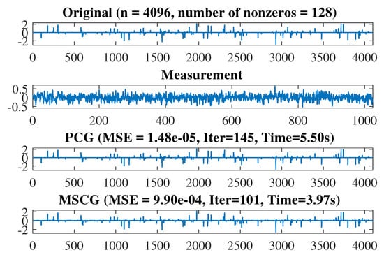
Figure 1. From top to bottom: the original image, the measurement, and the recovered signals b they PCG and MSCG methods.

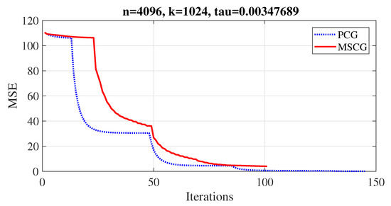
Figure 2. Iterations.

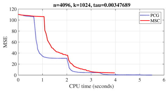
Figure 3. CPU time (seconds).

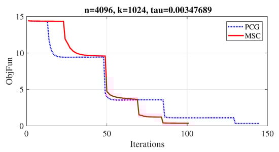
Figure 4. Iterations.

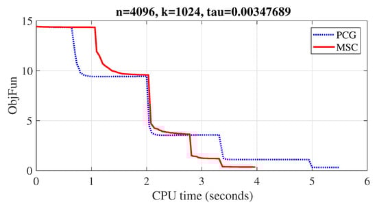
Figure 5. CPU time (seconds).

Table 10. Twenty five experiment results of ${\ell }_1-$norm regularization problem for MSCG and PCG methods.

	MSCG			PCG
	MSE	ITER	CPU(s)	MSE	ITER	CPU(s)
r = 0.1	9.90$\times {10}^{-4}$	101	3.97	1.48$\times {10}^{-5}$	145	5.5
	1.58$\times {10}^{-3}$	103	3.31	1.63$\times {10}^{-5}$	140	4.5
	7.68$\times {10}^{-4}$	113	3.17	1.30$\times {10}^{-5}$	133	3.47
	1.07$\times {10}^{-3}$	128	3.45	1.70$\times {10}^{-5}$	145	3.95
	1.23$\times {10}^{-3}$	122	3.2	1.38$\times {10}^{-5}$	143	3.77
	1.62$\times {10}^{-3}$	88	2.34	1.48$\times {10}^{-5}$	139	3.72
	1.66$\times {10}^{-3}$	114	3.19	1.84$\times {10}^{-5}$	132	3.59
	2.63$\times {10}^{-3}$	95	2.75	1.83$\times {10}^{-5}$	123	3.41
	1.16$\times {10}^{-3}$	99	2.67	1.22$\times {10}^{-5}$	113	2.92
	1.91$\times {10}^{-3}$	107	2.84	1.79$\times {10}^{-5}$	114	2.92
	2.18$\times {10}^{-3}$	106	2.69	2.09$\times {10}^{-5}$	110	2.81
	8.60$\times {10}^{-3}$	107	2.77	1.63$\times {10}^{-5}$	131	3.38
	1.33$\times {10}^{-3}$	102	2.78	1.27$\times {10}^{-5}$	143	3.78
	1.03$\times {10}^{-3}$	119	4.53	1.06$\times {10}^{-5}$	140	5.34
	1.15$\times {10}^{-3}$	110	3.03	1.48$\times {10}^{-5}$	135	3.61
	1.77$\times {10}^{-3}$	110	4.27	1.69$\times {10}^{-5}$	148	5.75
	1.36$\times {10}^{-3}$	103	3.83	1.47$\times {10}^{-5}$	114	4.34
	1.67$\times {10}^{-3}$	112	3.42	1.78$\times {10}^{-5}$	120	3.88
	1.21$\times {10}^{-3}$	107	4.38	1.47$\times {10}^{-5}$	114	4.91
	9.99$\times {10}^{-4}$	101	3.86	1.47$\times {10}^{-5}$	145	5.55
	1.58$\times {10}^{-3}$	103	2.78	1.63$\times {10}^{-5}$	140	3.7
	7.68$\times {10}^{-4}$	113	3.16	1.30$\times {10}^{-5}$	133	3.92
	1.07$\times {10}^{-3}$	128	4.77	1.70$\times {10}^{-5}$	145	5.59
	1.23$\times {10}^{-3}$	122	3.23	1.38$\times {10}^{-5}$	143	3.91
	1.62$\times {10}^{-3}$	88	2.41	1.48$\times {10}^{-5}$	139	3.81

5. Conclusions

In this paper, a modified three-term conjugate gradient method for solving monotone nonlinear equations with convex constraints was presented. The proposed algorithm is suitable for solving non-smooth equations because it requires no Jacobian information of the nonlinear equations. Under some assumptions, global convergence properties of the proposed method were proved. The numerical experiments presented clearly show how effective the MSCG algorithm is compared to the PCG and SATCGM methods of References [19,20] for the given constrained problems. In addition, the MSCG algorithm was shown to be effective in signal recovery problems.

References

- Kanzow, C.; Yamashita, N.; Fukushima, M. Levenberg–Marquardt methods with strong local convergence properties for solving nonlinear equations with convex constraints. J. Comput. Appl. Math. 2004, 172, 375–397. [Google Scholar] [CrossRef]
- Al-Baali, M.; Narushima, Y.; Yabe, H. A family of three term conjugate gradient methods with sufficient descent property for unconstrained optimization. Comput. Optim. Appl. 2015, 60, 89–110. [Google Scholar] [CrossRef]
- Hager, W.W.; Zhang, H. A survey of nonlinear conjugate gradient methods. Pac. J. Optim. 2006, 2, 35–58. [Google Scholar]
- Hager, W.; Zhang, H. A New Conjugate Gradient Method with Guaranteed Descent and an Efficient Line Search. SIAM J. Optim. 2005, 16, 170–192. [Google Scholar] [CrossRef]
- Narushima, Y. A smoothing conjugate gradient method for solving systems of nonsmooth equations. Appl. Math. Comput. 2013, 219, 8646–8655. [Google Scholar] [CrossRef]
- Narushima, Y.; Yabe, H.; Ford, J. A Three-Term Conjugate Gradient Method with Sufficient Descent Property for Unconstrained Optimization. SIAM J. Optim. 2011, 21, 212–230. [Google Scholar] [CrossRef]
- Sugiki, K.; Narushima, Y.; Yabe, H. Globally Convergent Three-Term Conjugate Gradient Methods that Use Secant Conditions and Generate Descent Search Directions for Unconstrained Optimization. J. Optim. Theory Appl. 2012, 153, 733–757. [Google Scholar] [CrossRef]
- Zhang, L.; Zhou, W.; Li, D. Some descent three-term conjugate gradient methods and their global convergence. Optim. Methods Softw. 2007, 22, 697–711. [Google Scholar] [CrossRef]
- Zhang, L.; Zhou, W.; Li, D.H. A descent modified Polak–Ribière–Polyak conjugate gradient method and its global convergence. IMA J. Numer. Anal. 2006, 26, 629–640. [Google Scholar] [CrossRef]
- Abubakar, A.B.; Kumam, P. An improved three-term derivative-free method for solving nonlinear equations. Comput. Appl. Math. 2018, 37, 6760–6773. [Google Scholar] [CrossRef]
- Abubakar, A.B.; Kumam, P. A descent Dai-Liao conjugate gradient method for nonlinear equations. Numer. Algorithms 2019, 81, 197–210. [Google Scholar] [CrossRef]
- Muhammed, A.A.; Kumam, P.; Abubakar, A.B.; Wakili, A.; Pakkaranang, N. A New Hybrid Spectral Gradient Projection Method for Monotone System of Nonlinear Equations with Convex Constraints. Thai J. Math. 2018, 16, 125–147. [Google Scholar]
- Mohammad, H.; Abubakar, A.B. A positive spectral gradient-like method for nonlinear monotone equations. Bull. Comput. Appl. Math. 2017, 5, 99–115. [Google Scholar]
- Wang, C.; Wang, Y.; Xu, C. A projection method for a system of nonlinear monotone equations with convex constraints. Math. Methods Oper. Res. 2007, 66, 33–46. [Google Scholar] [CrossRef]
- Wang, C.; Wang, Y. A superlinearly convergent projection method for constrained systems of nonlinear equations. J. Glob. Optim. 2009, 44, 283–296. [Google Scholar] [CrossRef]
- Solodov, M.; Svaiter, B. A New Projection Method for Variational Inequality Problems. SIAM J. Control Optim. 1999, 37, 765–776. [Google Scholar] [CrossRef]
- Xiao, Y.; Zhu, H. A conjugate gradient method to solve convex constrained monotone equations with applications in compressive sensing. J. Math. Anal. Appl. 2013, 405, 310–319. [Google Scholar] [CrossRef]
- Solodov, M.V.; Svaiter, B.F. A Globally Convergent Inexact Newton Method for Systems of Monotone Equations. In Reformulation: Nonsmooth, Piecewise Smooth, Semismooth and Smoothing Methods; Fukushima, M., Qi, L., Eds.; Applied Optimization; Springer: Boston, MA, USA; Berlin/Heidelberg, Germany, 1998; Volume 22, pp. 355–369. [Google Scholar]
- Liu, J.; Li, S. A projection method for convex constrained monotone nonlinear equations with applications. Comput. Math. Appl. 2015, 70, 2442–2453. [Google Scholar] [CrossRef]
- Wang, X.Y.; Li, S.J.; Kou, X.P. A self-adaptive three-term conjugate gradient method for monotone nonlinear equations with convex constraints. Calcolo 2016, 53, 133–145. [Google Scholar] [CrossRef]
- Zhou, W.; Li, D. Limited memory BFGS method for nonlinear monotone equations. J. Comput. Math. 2007, 25, 89–96. [Google Scholar]
- La Cruz, W. A spectral algorithm for large-scale systems of nonlinear monotone equations. Numer. Algorithms 2017, 76, 1109–1130. [Google Scholar] [CrossRef]
- Bing, Y.; Lin, G. An efficient implementation of Merrill’s method for sparse or partially separable systems of nonlinear equations. SIAM J. Optim. 1991, 1, 206–221. [Google Scholar] [CrossRef]
- Figueiredo, M.A.; Nowak, R.D. An EM algorithm for wavelet-based image restoration. IEEE Trans. Image Process. 2003, 12, 906–916. [Google Scholar] [CrossRef]
- Hale, E.T.; Yin, W.; Zhang, Y. A fixed-point continuation method for ℓ1-regularized minimization with applications to compressed sensing. CAAM TR07-07 Rice Univ. 2007, 43, 44. [Google Scholar]
- Beck, A.; Teboulle, M. A fast iterative shrinkage-thresholding algorithm for linear inverse problems. SIAM J. Imaging Sci. 2009, 2, 183–202. [Google Scholar] [CrossRef]
- Figueiredo, M.A.; Nowak, R.D.; Wright, S.J. Gradient projection for sparse reconstruction: Application to compressed sensing and other inverse problems. IEEE J. Sel. Top. Signal Process. 2007, 1, 586–597. [Google Scholar] [CrossRef]
- Van Den Berg, E.; Friedlander, M.P. Probing the Pareto frontier for basis pursuit solutions. SIAM J. Sci. Comput. 2008, 31, 890–912. [Google Scholar] [CrossRef]
- Birgin, E.G.; Martínez, J.M.; Raydan, M. Nonmonotone spectral projected gradient methods on convex sets. SIAM J. Optim. 2000, 10, 1196–1211. [Google Scholar] [CrossRef]
- Xiao, Y.; Wang, Q.; Hu, Q. Non-smooth equations based method for ℓ1-norm problems with applications to compressed sensing. Nonlinear Anal. Theory Methods Appl. 2011, 74, 3570–3577. [Google Scholar] [CrossRef]
- Pang, J.S. Inexact Newton methods for the nonlinear complementarity problem. Math. Program. 1986, 36, 54–71. [Google Scholar] [CrossRef]
© 2019 by the authors. Licensee MDPI, Basel, Switzerland. This article is an open access article distributed under the terms and conditions of the Creative Commons Attribution (CC BY) license (http://creativecommons.org/licenses/by/4.0/).