A Generic Family of Optimal Sixteenth-Order Multiple-Root Finders and Their Dynamics Underlying Purely Imaginary Extraneous Fixed Points

Abstract

A generic family of optimal sixteenth-order multiple-root finders are theoretically developed from general settings of weight functions under the known multiplicity. Special cases of rational weight functions are considered and relevant coefficient relations are derived in such a way that all the extraneous fixed points are purely imaginary. A number of schemes are constructed based on the selection of desired free parameters among the coefficient relations. Numerical and dynamical aspects on the convergence of such schemes are explored with tabulated computational results and illustrated attractor basins. Overall conclusion is drawn along with future work on a different family of optimal root-finders.

1. Introduction

Many nonlinear equations governing real-world natural phenomena cannot be solved exactly by virtue of their intrinsic complexities. It would be certainly an important matter to discuss methods for approximating such solutions of the nonlinear equations. The most widely accepted method under general circumstances is Newton’s method, which has quadratic convergence for a simple-root and linear convergence for a multiple-root. Other higher-order root-finders have been developed by many researchers [1,2,3,4,5,6,7,8,9] with optimal convergence satisfying Kung–Traub’s conjecture [10]. Several authors [10,11,12,13,14] have proposed optimal sixteenth-order simple-root finders, although their applications to real-life problems are limited due to the high degree of their algebraic complexities. Optimal sixteenth-order multiple-root finders are hardly found in the literature to the best of our knowledge at the time of writing this paper. It is not too much to emphasize the theoretical importance of developing optimal sixteenth-order multiple root-finders as well as to apply them to numerically solve real-world nonlinear problems.

In order to develop an optimal sixteenth-order multiple-root finders, we pursue a family of iterative methods equipped with generic weight functions of the form:

$$\left\{\begin{array}{l}{y}_n=x_n-m\frac{f\left(x_n\right)}{f^{\prime }\left(x_n\right)},\hfill \\ z_n=y_n-m{Q}_f\left(s\right)\frac{f\left(y_n\right)}{f^{\prime }\left(x_n\right)}=x_n-m\left[1+s{Q}_f\left(s\right)\right]\frac{f\left(x_n\right)}{f^{\prime }\left(x_n\right)},\hfill \\ w_n=z_n-m{K}_f(s,u)\frac{f\left(z_n\right)}{f^{\prime }\left(x_n\right)}=x_n-m\left[1+s{Q}_f\left(s\right)+su{K}_f(s,u)\right]\frac{f\left(x_n\right)}{f^{\prime }\left(x_n\right)},\hfill \\ x_{n+1}=w_n-m{J}_f(s,u,v)\frac{f\left(w_n\right)}{f^{\prime }\left(x_n\right)}=x_n-m\left[1+s{Q}_f\left(s\right)+su{K}_f(s,u)+suv{J}_f(s,u,v)\right]\frac{f\left(x_n\right)}{f^{\prime }\left(x_n\right)},\hfill \end{array}\right.$$

(1)

where $s={\left(\frac{f\left(y_n\right)}{f\left(x_n\right)}\right)}^{1/m},u={\left(\frac{f\left(z_n\right)}{f\left(y_n\right)}\right)}^{1/m},v={\left(\frac{f\left(w_n\right)}{f\left(z_n\right)}\right)}^{1/m}$; $Q_f:\mathbb{C}\to \mathbb{C}$ is analytic [15] in a neighborhood of 0, $K_f:{\mathbb{C}}^2\to \mathbb{C}$ holomorphic [16,17] in a neighborhood of $(0,0)$, and $J_f:{\mathbb{C}}^3\to \mathbb{C}$ holomorphic in a neighborhood of $(0,0,0)$. Since $s,u$ and v are respectively one-to-m multiple-valued functions, their principal analytic branches [15] are considered. Hence, for instance, it is convenient to treat s as a principal root given by $s=exp\left[\frac{1}{m}\mathrm{Log}\left(\frac{f\left(y_n\right)}{f\left(x_n\right)}\right)\right]$, with $\mathrm{Log}\left(\frac{f\left(y_n\right)}{f\left(x_n\right)}\right)=\mathrm{Log}\left|\frac{f\left(y_n\right)}{f\left(x_n\right)}\right|+i\mathrm{Arg}\left(\frac{f\left(y_n\right)}{f\left(x_n\right)}\right)$ for $-\pi <\mathrm{Arg}\left(\frac{f\left(y_n\right)}{f\left(x_n\right)}\right)\le \pi$; this convention of Arg(z) for $z\in \mathbb{C}$ agrees with that of Log[z] command of Mathematica [18] to be employed later in numerical experiments.

The case for $m=1$ has been recently developed by Geum–Kim–Neta [19]. Many other existing cases for $m=1$ are special cases of (1) with appropriate forms of weight functions $Q_f,K_f$, and $J_f$; for example, the case developed in [10] uses the following weight functions:

$$\left\{\begin{array}{c}{Q}_f\left(s\right)=\frac{1}{{(1-s)}^2},\hfill \\ K_f(s,u)=\frac{1+(1-u)s^2}{{(1-s)}^2(1-u){(1-su)}^2},\hfill \\ J_f(s,u,v)=\frac{-1+2s{u}^2(v-1)+s^4(u-1)u^2(v-1)(uv-1)+s^2[uv-1-u^3(v^2-1)]}{{(1-s)}^2(u-1){(su-1)}^2(v-1)(uv-1){(suv-1)}^2}.\hfill \end{array}\right.$$

(2)

One goal of this paper is to construct a family of optimal sixteenth-order multiple-root finders by characterizing the generic forms of weight functions $Q_f\left(s\right)$, $K_f(s,u)$, and $J_f(s,u,v)$. The other goal is to investigate the convergence behavior by exploring their numerical behavior and dynamics through basins of attractions [20] underlying the extraneous fixed points [21] when $f\left(z\right)={(z-a)}^m{(z-b)}^m$ is applied. In view of the right side of final substep of (1), we can conveniently locate extraneous fixed points from the roots of the weight function $m[1+s{Q}_f\left(s\right)+su{K}_f(s,u)+suv{J}_f(s,u,v)]$.

A motivation undertaking this research is to investigate the local and global characters on the convergence of proposed family of methods (1). The local convergence of an iterative method for solving nonlinear equations is usually guaranteed with an initial guess taken in a sufficiently close neighborhood of the sought zero. On the other hand, effective information on its global convergence is hardly achieved under general circumstances. We can obtain useful information on the global convergence from attractor basins through which relevant dynamics is worth exploring. Especially the dynamics underlying the extraneous fixed points (to be described in Section 3) would influence the dynamical behavior of the iterative methods by the presence of possible attractive, indifferent, repulsive, and other chaotic orbits. One way of reducing such influence is to control the location of the extraneous fixed points. We prefer the location to be the imaginary axis that divides the entire complex plane into two symmetrical half-planes. The dynamics underlying the extraneous fixed points on the imaginary axis would be less influenced by the presence of the possible periodic or chaotic attractors.

The main theorem is presented in Section 2 with required constraints on weight functions, $Q_f$, $K_f$, and $J_f$ to achieve the convergence order of 16. Section 2 discusses special cases of rational weight functions. Section 3 extensively investigates the purely imaginary extraneous fixed points and investigates their stabilities. Section 4 presents numerical experiments as well as the relevant dynamics, while Section 5 states the overall conclusions along with the short description of future work.

2. Methods and Special Cases

A main theorem on the convergence of (1) is established here with the error equation and relationships among generic weight functions $Q_f\left(s\right)$, $K_f(s,u)$, and $J_f(s,u,v)$:

Theorem 1.

Suppose that $f:\mathbb{C}\to \mathbb{C}$ has a multiple root α of multiplicity $m\ge 1$ and is analytic in a neighborhood of α. Let $c_j=\frac{m!}{(m-1+j)!}\frac{f^{(m-1+j)}\left(\alpha \right)}{f\left(m\right)\left(\alpha \right)}$ for $j=2,3,\cdots$. Let $x_0$ be an initial guess selected in a sufficiently small region containing α. Assume $L_f:\mathbb{C}\to \mathbb{C}$ is analytic in a neighborhood of 0. Let $Q_i=\frac{1}{i!}\frac{d^i}{d{s}^i}{Q}_f\left(s\right){|}_{(s=0)}$ for $0\le i\le 6$. Let $K_f:{\mathbb{C}}^2\to \mathbb{C}$ be holomorphic in a neighborhood of $(0,0)$. Let $J_f:{\mathbb{C}}^3\to \mathbb{C}$ be holomorphic in a neighborhood of $(0,0,0)$. Let $K_{ij}=\frac{1}{i!j!}\frac{{\partial }^{i+j}}{\partial s^i\partial u^j}{K}_f(s,u){|}_{(s=0,u=0)}$ for $0\le i\le 12$ and $0\le j\le 6$. Let $J_{ijk}=\frac{1}{i!j!k!}\frac{{\partial }^{i+j+k}}{\partial s^i\partial u^j\partial v^j}{J}_f(s,u,v){|}_{(s=0,u=0,v=0)}$ for $0\le i\le 8$, $0\le j\le 4$ and $0\le k\le 2$. If $Q_0=1,Q_1=2,K_{00}=1,K_{10}=2,K_{01}=1,K_{20}=1+Q_2,K_{11}=4,K_{30}=-4+2Q_2+Q_3$, $J_{000}=1,J_{100}=2,J_{200}=1+Q_2,J_{010}=1,J_{110}=4,J_{300}=-4+2Q_2+Q_3,J_{001}=1,J_{020}=K_{02},J_{210}=1+K_{21},J_{400}=K_{40},J_{101}=2,J_{120}=2+K_{12},J_{310}=-4+K_{31}+2Q_2,J_{500}=K_{50},J_{011}=2,J_{201}=1+Q_2,J_{030}=-1+K_{02}+K_{03},J_{220}=1+K_{21}+K_{22}-Q_2,J_{410}=-3+K_{40}+K_{41}+Q_2-Q_4,J_{600}=K_{60},J_{111}=8,J_{301}=-4+2Q_2+Q_3,J_{130}=-4+2K_{02}+K_{12}+K_{13},J_{320}=-6+2K_{21}+K_{31}+K_{32}-2Q_2-Q_3,J_{510}=6+2K_{40}+K_{50}+K_{51}-3Q_3-2Q_4-Q_5,J_{700}=K_{70}$ are fulfilled, then Scheme (1) leads to an optimal class of sixteenth-order multiple-root finders possessing the following error equation: with $e_n=x_n-\alpha$ for $n=0,1,2,\cdots ,$

$$e_{n+1}=\frac{1}{3456m^{15}}{c}_2(\rho c_2^2-2m{c}_3)\left[{\beta }_0{c}_2^4+{\beta }_1{c}_2^2{c}_3+12m^2(K_{02}-1)c_3^2-12m^2{c}_2{c}_4\right]\Psi e_n^{16}+O\left(e_n^{17}\right),$$

(3)

where $\rho =9+m-2Q_2$, ${\beta }_0=(-431+12K_{40}-7m^2+6m(-17+Q_2)+102Q_2-24Q_3-12Q_4+6K_{21}\rho +3K_{02}{\rho }^2),{\beta }_1=-12m(-17+K_{21}-2m+Q_2+K_{02}\rho )$, $\Psi ={\Delta }_1{c}_2^8+{\Delta }_2{c}_2^6{c}_3+{\Delta }_3{c}_2^5{c}_4+{\Delta }_4{c}_2^3{c}_3{c}_4+{\Delta }_5{c}_2^4+{\Delta }_6{c}_2^2+{\Delta }_7{c}_3^4+{\Delta }_8{c}_2{c}_3^2{c}_4$,

${\Delta }_1=(-255124+144J_{800}-144K_{80}-122577m-23941m^2-2199m^3-79m^4+24K_{40}(472+93m+5m^2)-72(17+m)Q_2^3-576Q_3^2+Q_3(48(-566+6K_{40}-117m-7m^2)-576Q_4)+24(-485+6K_{40}-108m-7m^2)Q_4-144Q_4^2+Q_2^2(36(-87+14m+m^2)+288Q_3+144Q_4)+Q_2(18(5300+1529m+172m^2+7m^3-8K_{40}(18+m))+144(35+m)Q_3+72(29+m)Q_4)+18{\rho }^3\sigma +6\rho (12J_{610}-12(2K_{50}+K_{60}+K_{61}-2Q_5-Q_6)+J_{211}(-12K_{40}+{\sigma }_2)+2K_{21}(-J_{002}{\sigma }_2+{\sigma }_3+6{\eta }_0))+{\rho }^2(36J_{420}-36J_{211}{K}_{21}+36J_{002}{K}_{21}^2-72K_{31}-36J_{021}{K}_{40}-36K_{41}-36K_{42}+3J_{021}{\sigma }_2+6K_{02}(-6J_{401}+12J_{002}{K}_{40}-J_{002}{\sigma }_2+{\sigma }_3))+12J_{401}{\sigma }_7+J_{002}{\sigma }_7^2+9{\rho }^4\tau )$,

${\Delta }_2=m(144(Q_2^3-2Q_5-Q_6)+288Q_3(-K_{21}+(39+4m)-K_{02}\rho )+144Q_2^2(-2K_{21}-(7+m)-K_{02}\rho )+144Q_4(-K_{21}+4(9+m)-K_{02}\rho )+Q_2(144K_{21}(58+5m)-36(1529-8K_{40}+m(302+17m))-288Q_3-144Q_4+144K_{02}(38+3m)\rho )-108{\rho }^2\sigma +6(40859-24J_{610}+48K_{50}+24K_{60}+24K_{61}+24K_{40}(-31+J_{211}-3m)+m(14864+m(1933+88m))-2J_{211}{\sigma }_8)-72{\rho }^3\tau -24{\rho }_2(J_{002}{\sigma }_2-6{\eta }_0)-24K_{21}(1309+m(267+14m)-J_{002}{\sigma }_8+6{\eta }_0)+\rho (144J_{211}{K}_{21}-144J_{002}{K}_{21}^2+12(-12J_{420}+12(2K_{31}+J_{021}{K}_{40}+K_{41}+K_{42})-J_{021}{\sigma }_4)-12K_{02}(1781+m(360+19m)-2J_{002}{\sigma }_4+12{\eta }_0)))$,

${\Delta }_3=12m^2(6(63+5m)Q_2-48Q_3-24Q_4+6(J_{211}+K_{21}-2J_{002}{K}_{21})\rho -(1645-12J_{401}+12(-1+2J_{002})K_{40}+372m+23m^2-2J_{002}{\sigma }_2)+3{\rho }^2{\sigma }_5)$,

${\Delta }_4=144m^3(-3Q_2+(53-J_{211}+(-1+2J_{002})K_{21}+6m-2J_{002}{\rho }_2)-\rho {\sigma }_5)$,

${\Delta }_5=72\rho m^3{c}_5+12m^2{c}_3^2((-12K_{21}(J_{211}-4(10+m))+K_{02}(4778-12J_{401}+m(990+52m))+3(-1929+4J_{401}+4J_{420}-8K_{31}+8K_{40}-4K_{41}-4K_{42}-476m-31m^2+2J_{211}(43+5m)+J_{021}(115+22m+m^2)))-6(-88+121J_{021}+4J_{211}+232K_{02}+8K_{21}+(-10+13J_{021}+22K_{02})m+2J_{002}(51-4K_{21}+5m))Q_2+12(1+J_{002}+3J_{021}+6K_{02})Q_2^2+18\rho \sigma +18{\rho }^2\tau +Q_4(12(-2+K_{02})+12{\eta }_1)+Q_3(24(-2+K_{02})+24{\eta }_1)-J_{021}{\eta }_2+{\eta }_1((2165-12K_{40}+m(510+31m))+{\eta }_2))$,

${\Delta }_6=72m^3(2(-1+J_{002})m{c}_4^2-2m{c}_3{c}_5+c_3^3(2Q_2(-1+6K_{02})-2K_{02}(49-J_{211}+5m+2J_{002}{\rho }_3)+(85-2J_{211}-2J_{230}+4K_{12}-4K_{21}+4J_{002}(K_{21}-{\rho }_2)+2K_{22}+2K_{23}+11m+2J_{021}{\rho }_3)-4\rho \tau ))$,

${\Delta }_7=144m^4(-1+J_{002}+J_{021}+J_{040}-K_{03}-K_{04}+(2-{\eta }_1)K_{02}+J_{002}{K}_{02}^2)$, ${\Delta }_8=144m^4(-3+{\eta }_1+(1-2J_{002})K_{02})$,

$\tau =J_{040}-J_{021}{K}_{02}+J_{002}{K}_{02}^2-K_{03}-K_{04},{\rho }_2=17+2m-Q_2,{\rho }_3=-26+K_{21}-3m+3Q_2,\sigma =J_{230}-J_{211}{K}_{02}-2K_{12}-J_{021}{K}_{21}+2J_{002}{K}_{02}{K}_{21}-K_{22}-K_{23},{\sigma }_2=431+7m^2-6m(-17+Q_2)-102Q_2+24Q_3+12Q_4,{\sigma }_3=472+5m^2+m(93-6Q_2)-108Q_2+12Q_3+6Q_4,{\sigma }_4=890+13m^2-231Q_2+6Q_2^2-3m(-69+7Q_2)+24Q_3+12Q_4,{\sigma }_5=J_{021}+K_{02}-2J_{002}{K}_{02},{\sigma }_6=-1255+6K_{40}-288m-17m^2+363Q_2+39m{Q}_2-18Q_2^2-12Q_3-6Q_4,{\sigma }_7=431-12K_{40}+7m^2-6m(-17+Q_2)-102Q_2+24Q_3+12Q_4,{\sigma }_8=1349+19m^2+m(312-36Q_2)-360Q_2+12Q_2^2+24Q_3+12Q_4,{\eta }_0=-J_{401}+2J_{002}{K}_{40},{\eta }_1=2J_{002}+J_{021},{\eta }_2=6K_{21}^2-6K_{21}(43+5m)+2{\sigma }_6{K}_{02}$.

Proof. 

Since Scheme (1) employs five functional evaluations, namely, $f^{\prime }\left(x_n\right)$, $f\left(x_n\right)$, $f\left(y_n\right)$, $f\left(z_n\right)$, and $f\left(w_n\right)$, optimality can be achieved if the corresponding convergence order is 16. In order to induce the desired order of convergence, we begin by the 16th-order Taylor series expansion of $f\left(x_n\right)$ about $\alpha$:

$$f\left(x_n\right)=\frac{f^{\prime }\left(\alpha \right)}{m!}{e}_n^m\{1+\sum _{i=2}^{17}{c}_i{e}_n^{i-1}+O\left(e_n^{17}\right)\}.$$

(4)

It follows that

$$f^{\prime }\left(x_n\right)=\frac{f^{\prime }\left(\alpha \right)}{(m-1)!}{e}_n^{m-1}\{1+\sum _{i=2}^{16}i\frac{m+i-1}{m}{c}_i{e}_n^{i-1}+O\left(e_n^{16}\right)\}.$$

(5)

For brevity of notation, we abbreviate $e_n$ as e. Using Mathematica [18], we find:

$$y_n=x_n-m\frac{f\left(x_n\right)}{f^{\prime }\left(x_n\right)}=\alpha +\frac{c_2}{m}{e}^2+\frac{(-(m+1)c_2^2+2m{c}_3)}{m^2}{e}^3+\frac{Y_4}{m^3}{e}^4+\sum _{i=5}^{16}\frac{Y_i}{m^{i-1}}{e}_n^i+O\left(e^{17}\right),$$

(6)

where $Y_4={(1+m)}^2{c}_2^3-m(4+3m)c_2{c}_3+3m^2{c}_4$ and $Y_i=Y_i(c_2,c_3,\cdots ,c_{16})$ for $5\le i\le 16$.

After a lengthy computation using the fact that $f\left(y_n\right)=f\left(x_n\right){|}_{e_n\to (y_n-\alpha )}$, we get:

$$s={\left(\frac{f\left(y_n\right)}{f\left(x_n\right)}\right)}^{1/m}=\frac{c_2}{m}e+\frac{(-(m+2)c_2^2+2m{c}_3)}{m^2}{e}^2+\frac{{\gamma }_3}{2m^3}{e}^3+\sum _{i=4}^{15}{E}_i{e}^i+O\left(e^{16}\right),$$

(7)

where ${\gamma }_3=(7+7m+2m^2)c_2^3-2m(7+3m)c_2{c}_3+6m^2{c}_4$, $E_i=E_i(c_2,c_3,\cdots ,c_{16})$ for $4\le i\le 15$.

In the third substep of Scheme (1), $w_n=O\left(e^8\right)$ can be achieved based on Kung–Traub’s conjecture. To reflect the effect on $w_n$ from $z_n$ in the second substep, we need to expand $z_n$ up to eighth-order terms; hence, we carry out a sixth-order Taylor expansion of $Q_f\left(s\right)$ about 0 by noting that $s=O\left(e\right)$ and $\frac{f\left(y_n\right)}{f^{\prime }\left(x_n\right)}=O\left(e^2\right)$:

$$Q_f\left(s\right)=Q_0+Q_{1}s+Q_2{s}^2+Q_3{s}^3+Q_4{s}^4+Q_5{s}^5+Q_6{s}^6+O\left(e^7\right),$$

(8)

where $Q_j=\frac{1}{j!}\frac{d^j}{d{s}^j}{Q}_f\left(s\right)$ for $0\le j\le 6$. As a result, we come up with:

$$z_n=x_n-m{Q}_f\left(s\right)\frac{f\left(y_n\right)}{f^{\prime }\left(x_n\right)}=\alpha +\frac{(1-Q_0)}{m}{e}^2+\frac{{\mu }_3}{m^2}{e}^3+\sum _{i=4}^{16}{W}_i{e}^i+O\left(e^{17}\right),$$

where ${\mu }_3=(-1+m(Q_0-1)+3Q_0-Q_1)c_2^2-2m(Q_0-1)c_3$ and $W_i=W_i(c_2,c_3,\cdots ,c_{16},Q_0,\cdots ,Q_6)$ for $4\le i\le 16$. Selecting $Q_0=1$ and $Q_1=2$ leads us to an expression:

$$z_n=\alpha +\frac{c_2(\rho c_2^2-2m{c}_3)}{m^2}{e}^4+\sum _{i=5}^{16}{W}_i{e}^i+O\left(e^{17}\right).$$

(9)

By a lengthy computation using the fact that $f\left(z_n\right)=f\left(x_n\right){|}_{e_n\to (z_n-\alpha )}$, we deduce:

$$u={\left(\frac{f\left(z_n\right)}{f\left(y_n\right)}\right)}^{1/m}=\frac{(\rho c_2^2-2m{c}_3)}{2m^2}{e}^2+\frac{{\delta }_3}{3m^3}{e}^3+\sum _{i=4}^{16}{G}_i{e}^i+O\left(e^{17}\right),$$

(10)

where ${\delta }_3=(49+2m^2+m(27-6Q_2)-18Q_2+3Q_3)c_2^3-6m\rho c_2{c}_3+6m^2{c}_4$ and $G_i=G_i(c_2,c_3,\cdots ,c_{16},Q_2,\cdots ,Q_6)$ for $4\le i\le 16$.

In the last substep of Scheme (1), $x_{n+1}=O\left(e^{16}\right)$ can be achieved based on Kung-Traub’s conjecture. To reflect the effect on $x_{n+1}$ from $w_n$ in the third substep, we need to expand $w_n$ up to sixteenth-order terms; hence, we carry out a 12th-order Taylor expansion of $K_f(s,u)$ about $(0,0)$ by noting that: $s=O\left(e\right),u=O\left(e^2\right)$ and $\frac{f\left(z_n\right)}{f^{\prime }\left(x_n\right)}=O\left(e^4\right)$ with $K_{ij}=0$ satisfying $i+2j>12$ for all $0\le i\le 12,0\le j\le 6$:

$$\begin{array}{r}\hfill K_f(s,u)=K_{00}+K_{10}s+K_{20}{s}^2+K_{30}{s}^3+K_{40}{s}^4+K_{50}{s}^5+K_{60}{s}^6+K_{70}{s}^7+K_{80}{s}^8+K_{90}{s}^9+K_{100}{s}^{10}+K_{110}{s}^{11}+\\ \hfill K_{120}{s}^{12}+(K_{01}+K_{11}s+K_{21}{s}^2+K_{31}{s}^3+K_{41}{s}^4+K_{51}{s}^5+K_{61}{s}^6+K_{71}{s}^7+K_{81}{s}^8+K_{91}{s}^9+K_{101}{s}^{10})u+\\ \hfill (K_{02}+K_{12}s+K_{22}{s}^2+K_{32}{s}^3+K_{42}{s}^4+K_{52}{s}^5+K_{62}{s}^6+K_{72}{s}^7+K_{82}{s}^8)u^2+\\ \hfill (K_{03}+K_{13}s+K_{23}{s}^2+K_{33}{s}^3+K_{43}{s}^4+K_{53}{s}^5+K_{63}{s}^6)u^3+\\ \hfill (K_{04}+K_{14}s+K_{24}{s}^2+K_{34}{s}^3+K_{44}{s}^4)u^4+(K_{05}+K_{15}s+K_{25}{s}^2)u^5+K_{06}{u}^6+O\left(e^{13}\right).\end{array}$$

(11)

Substituting $z_n,f\left(x_n\right),f\left(y_n\right),f\left(z_n\right),f^{\prime }\left(x_n\right)$, and $K_f(s,u)$ into the third substep of (1) leads us to:

$$w_n=z_n-m{K}_f(s,u)·\frac{f\left(z_n\right)}{f^{\prime }\left(x_n\right)}=\alpha +\frac{(1-K_{00})c_2(\rho c_2^2-2m{c}_3)}{2m^3}{e}^4+\sum _{i=5}^{16}{\Gamma }_i{e}^i+O\left(e^{17}\right),$$

(12)

where ${\Gamma }_i={\Gamma }_i(c_2,c_3,\cdots ,c_{16},Q_2,\cdots ,Q_6,K_{j\ell })$, for $5\le i\le 16$, $0\le j\le 12$ and $0\le \ell \le 6$. Thus $K_{00}=1$ immediately annihilates the fourth-order term. Substituting $K_{00}=1$ into ${\Gamma }_5=0$ and solving for $K_{10}$, we find:

$$K_{10}=2.$$

(13)

Continuing the algebraic operations in this manner at the i-th ($6\le i\le 7$) stage with known values of $K_{j\ell }$, we solve ${\Gamma }_i=0$ for remaining $K_{j\ell }$ to find:

$$K_{20}=1+Q_2,K_{01}=1.$$

(14)

Substituting $K_{00}=1,K_{10}=2,K_{20}=1+Q_2,K_{01}=1$ into (12) and simplifying we find:

$$v={\left(\frac{f\left(w_n\right)}{f\left(z_n\right)}\right)}^{1/m}=-\frac{\left[{\beta }_0{c}_2^4+{\beta }_1{c}_2^2{c}_3+12m^2(K_{02}-1)c_3^2-12m^2{c}_2{c}_4\right]}{12m^4}{e}^4+\sum _{i=5}^{16}{T}_i{e}^i+O\left(e^{17}\right),$$

(15)

where ${\beta }_0$ and ${\beta }_1$ are described in (3) and $T_i=T_i(c_2,c_3,\cdots ,c_{16},Q_2,\cdots ,Q_6)$ for $5\le i\le 16$.

To compute the last substep of Scheme (1), it is necessary to have an eighth-order Taylor expansion of $J_f(s,u,v)$ about $(0,0,0)$ due to the fact that $\frac{f\left(w_n\right)}{f^{\prime }\left(x_n\right)}=O\left(e^8\right)$. It suffices to expand $J_f$ up to eighth-, fourth-, and second-order terms in $s,u,v$ in order, by noting that $s=O\left(e\right),u=O\left(e^2\right),v=O\left(e^4\right)$ with $J_{ijk}=0$ satisfying $i+2j+4k>8$ for all $0\le i\le 8,0\le j\le 4,0\le k\le 2$:

$$\begin{array}{r}\hfill J_f(s,u,v)=J_{000}+J_{100}s+J_{200}{s}^2+J_{300}{s}^3+J_{400}{s}^4+J_{500}{s}^5+J_{600}{s}^6+J_{700}{s}^7+J_{800}{s}^8+(J_{010}+J_{110}s+J_{210}{s}^2+\\ \hfill J_{310}{s}^3+J_{410}{s}^4+J_{510}{s}^5+J_{610}{s}^6)u+(J_{020}+J_{120}s+J_{220}{s}^2+J_{320}{s}^3+J_{420}{s}^4)u^2+(J_{030}+J_{130}s+J_{230}{s}^2)u^3+\\ \hfill J_{040}{u}^4+(J_{001}+J_{101}s+J_{201}{s}^2+J_{301}{s}^3+J_{401}{s}^4+(J_{011}+J_{111}s+J_{211}{s}^2)u+J_{021}{u}^2)v+J_{002}{v}^2.\end{array}$$

(16)

Substituting $w_n,f\left(x_n\right),f\left(y_n\right),f\left(z_n\right),f\left(w_n\right),f^{\prime }\left(x_n\right)$ and $J_f(s,u,v)$ in (1), we arrive at:

$$x_{n+1}=w_n-m{J}_f(s,u,v)·\frac{f\left(w_n\right)}{f^{\prime }\left(x_n\right)}=\alpha +\varphi e^8+\sum _{i=9}^{16}{\Omega }_i{e}^i+O\left(e^{17}\right),$$

(17)

where $\varphi =\frac{1}{24m^7}(1-J_{000})c_2(\rho c_2^2-2m{c}_3)\left[{\beta }_0{c}_2^4+{\beta }_1{c}_2^2{c}_3+12m^2(K_{02}-1)c_3^2-12m^2{c}_2{c}_4\right]$ and ${\Omega }_i=$${\Omega }_i(c_2,c_3,\cdots ,c_{16},$$Q_2,\cdots ,Q_6,K_{\delta \theta },J_{jk\ell }$), for $9\le i\le 16$, $0\le \delta \le 12$, $0\le \theta \le 6$, $0\le j\le 8$, $0\le k\le 4$, $0\le \ell \le 2$.

Since $J_{000}=1$ makes $\varphi =0$, we substitute $J_{000}=1$ into ${\Omega }_9=0$ and solve for $J_{100}$ to find:

$$J_{100}=2.$$

(18)

Continuing the algebraic operations in the same manner at the i-th ($10\le i\le 15$) stage with known values of $J_{jk\ell }$, we solve ${\Omega }_i=0$ for remaining $J_{jk\ell }$ to find:

$$\left\{\begin{array}{l}{J}_{200}=1+Q_2,J_{010}=1,J_{110}=4,J_{300}=-4+2Q_2+Q_3,J_{001}=1,J_{020}=K_{02},J_{210}=1+K_{21},\hfill \\ J_{400}=K_{40},J_{101}=2,J_{120}=2+K_{12},J_{310}=-4+K_{31}+2Q_2,J_{500}=K_{50},J_{011}=2,J_{201}=1+Q_2,\hfill \\ J_{111}=8,J_{030}=-1+K_{02}+K_{03},J_{220}=1+K_{21}+K_{22}-Q_2,J_{410}=-3+K_{40}+K_{41}+Q_2-Q_4,\hfill \\ J_{301}=-4+2Q_2+Q_3,J_{130}=-4+2K_{02}+K_{12}+K_{13},J_{320}=-6+2K_{21}+K_{31}+K_{32}-2Q_2-Q_3,\hfill \\ J_{600}=K_{60},J_{510}=6+2K_{40}+K_{50}+K_{51}-3Q_3-2Q_4-Q_5,J_{700}=K_{70}.\hfill \end{array}\right.$$

(19)

Upon substituting Relation (19) into ${\Omega }_{16}$, we finally obtain:

$${\Omega }_{16}=\frac{1}{3456m^{15}}{c}_2(\rho c_2^2-2m{c}_3)\left[{\beta }_0{c}_2^4+{\beta }_1{c}_2^2{c}_3+12m^2(K_{02}-1)c_3^2-12m^2{c}_2{c}_4\right]\Psi ,$$

(20)

where $\rho$, ${\beta }_0,{\beta }_1$, and $\Psi$ as described in (3). This completes the proof. ☐

Remark 1.

Theorem 1 clearly reflects the case for $m=1$ with the same constraints on weight functions $Q_f,K_f,J_f$ studied in [19].

Special Cases of Weight Functions

Theorem 1 enables us to obtain $Q_f\left(s\right)$, $K_f(s,u)$, and $J_f(s,u,v)$ by means of Taylor polynomials:

$$\left\{\begin{array}{l}{Q}_f\left(s\right)=1+2s+Q_2{s}^2+Q_3{s}^3+Q_4{s}^4+Q_5{s}^5+Q_6{s}^6+O\left(e^7\right),\hfill \\ K_f(s,u)=1+2s+(1+Q_2)s^2+(2Q_2+Q_3-4)s^3+K_{40}{s}^4+K_{50}{s}^5+K_{60}{s}^6+K_{70}{s}^7+K_{80}{s}^8\hfill \\ +K_{90}{s}^9+K_{100}{s}^{10}+K_{110}{s}^{11}+K_{120}{s}^{12}+(1+4s+K_{21}{s}^2+K_{31}{s}^3+K_{41}{s}^4+K_{51}{s}^5+K_{61}{s}^6\hfill \\ +K_{71}{s}^7+K_{81}{s}^8+K_{91}{s}^9+K_{101}{s}^{10})u+(K_{02}+K_{12}s+K_{22}{s}^2+K_{32}{s}^3+K_{42}{s}^4+K_{52}{s}^5\hfill \\ +K_6{s}^6+K_{72}{s}^7+K_{82}{s}^8)u^2+(K_{03}+K_{13}s+K_{23}{s}^2+K_{33}{s}^3+K_{43}{s}^4+K_{53}{s}^5+K_{63}{s}^6)u^3\hfill \\ +(K_{04}+K_{14}s+K_{24}{s}^2+K_{34}{s}^3+K_{44}{s}^4)u^4+(K_{05}+K_{15}s+K_{25}{s}^2)u^5+K_{06}{u}^6+O\left(e^{13}\right),\hfill \\ J_f(s,u,v)=1+2s+(1+Q_2)s^2+(2Q_2+Q_3-4)s^3+K_{40}{s}^4+K_{50}{s}^5+K_{60}{s}^6+K_{70}{s}^7+J_{800}{s}^8\hfill \\ +(1+4s+(1+K_{21})s^2+(K_{31}+2Q_2-4)s^3+(K_{40}+K_{41}-3+Q_2-Q_4)s^4+(2K_{40}+K_{50}+K_{51}+6\hfill \\ -3Q_3-2Q_4-Q_5)s^5+J_{610}{s}^6)u+(K_{02}+(2+K_{12})s+(K_{21}+K_{22}-Q_2+1)s^2+(2K_{21}+K_{31}+K_{32}-6\hfill \\ -2Q_2-Q_3)s^3+J_{420}{s}^4)u^2+(K_{02}+K_{03}-1+(2K_{02}+K_{12}+K_{13}-4)s+J_{230}{s}^2)u^3+J_{040}{u}^4\hfill \\ +(1+2s+(1+Q_2)s^2+(2Q_2+Q_3-4)s^3+J_{401}{s}^4+(2+8s+J_{211}{s}^2)u+J_{021}{u}^2)v+J_{002}{v}^2+O\left(e^9\right),\hfill \end{array}\right.$$

(21)

where parameters $Q_2$–$Q_6$, $K_{40},K_{50},K_{60},K_{70},K_{80},K_{90},K_{100},K_{110},K_{120},K_{21},K_{31},K_{41},K_{51},K_{61},K_{71},K_{81}$, $K_{91},K_{101}$, $K_{02}$, $K_{12}$, $K_{22}$, $K_{32},K_{42},K_{52},K_{62},K_{72},K_{82}$, $K_{03},K_{13},K_{23},K_{33},K_{43},K_{53},K_{63},K_{04},K_{14},K_{24},K_{34},K_{44}$, $K_{05},K_{15},K_{25},K_{06}$ and $J_{040},J_{002},J_{021},J_{211},J_{230},J_{401},J_{420},J_{610},J_{800}$ may be free.

Although various forms of weight functions $Q_f\left(s\right)$, $K_f(s,u)$ and $J_f(s,u,v)$ are available, in the current study we limit ourselves to all three weight functions in the form of rational functions, leading us to possible purely imaginary extraneous fixed points when $f\left(z\right)={(z^2-1)}^m$ is employed. In the current study, we will consider two special cases described below:

The first case below will represent the best scheme, W3G7, studied in [19] only for $m=1$.

Case 1:

$$\left\{\begin{array}{cc}{Q}_f\left(s\right)\hfill & =\frac{1}{1-2s},\hfill \\ K_f(s,u)\hfill & =Q_f\left(s\right)·\frac{{(s-1)}^2}{1-2s-u+2s^{2}u},\hfill \\ J_f(s,u,v)\hfill & =K_f(s,u)·\frac{1+{\sum }_{i=1}^3{q}_i{s}^i+u{\sum }_{i=4}^8{q}_i{s}^{i-4}+u^2{\sum }_{i=9}^{14}{q}_i{s}^{i-9}+u^3{\sum }_{i=15}^{21}{q}_i{s}^{i-15}}{{\mathcal{A}}_1(s,u)+v·({\sum }_{i=22}^{25}{r}_i{s}^{i-22}+u(r_{26}+r_{27}s+\lambda s^2)},\hfill \end{array}\right.$$

(22)

where

$$\left\{\begin{array}{c}{q}_9=q_{12}=q_{13}=q_{17}=q_{18}=q_{19}=q_{20}=r_9=r_{10}=r_{19}=r_{20}=0,\hfill \\ q_1=\frac{-3055820263252-76497245\lambda }{142682111242},q_2=\frac{56884034112404+44614515451\lambda }{285364222484},\hfill \\ q_3=\frac{-45802209949332-44308526471\lambda }{142682111242},q_4=-\frac{3(17778426888128+67929066997\lambda )}{1426821112420},\hfill \\ q_5=\frac{2(21034820227211+132665343294\lambda )}{356705278105},q_6=\frac{-1589080655012451+134087681464\lambda }{142682111242},\hfill \\ q_7=\frac{2(-780300304419180+71852971399\lambda )}{71341055621},q_8=\frac{12288(-727219117761+128167952\lambda )}{71341055621},\hfill \\ q_{10}=2,q_{11}=\frac{2(-741727036224277+126275739062\lambda )}{71341055621},\hfill \\ q_{14}=-\frac{8192(-3964538065856+615849113\lambda )}{71341055621},q_{15}=\frac{8(-226231159891830+34083208621\lambda )}{71341055621},\hfill \\ q_{16}=-\frac{24(-908116719056544+136634733499\lambda )}{356705278105},q_{21}=\frac{131072(-918470889768+136352293\lambda )}{356705278105},\hfill \\ r_1=q_1,r_2=q_2,r_3=q_3,r_4=q_4,r_5=q_5,r_6=q_6-1,r_7=q_7-q_1-2,r_8=q_8+\frac{q_3}{2},\hfill \\ r_{11}=\frac{-29558910226378916+5256346708371\lambda }{1426821112420},r_{12}=\frac{-55018830261476-109759858153\lambda }{142682111242},\hfill \\ r_{13}=\frac{25(-75694849962572+11301475999\lambda )}{71341055621},r_{14}=-\frac{4096(-1500792372416+228734011\lambda )}{15508925135},\hfill \\ r_{15}=q_{15},r_{16}=\frac{43641510974266076-6354680006961\lambda }{713410556210},r_{17}=-\frac{2(-1060205894022116+202907726307\lambda )}{71341055621},\hfill \\ r_{18}=\frac{2(-2870055173156756+475573395275\lambda )}{71341055621},r_{21}=\frac{q_{21}}{2},r_{22}=-1,r_{23}=-q_1,r_{24}=-q_2,\hfill \\ r_{25}=-q_3,r_{26}=-1-q_4,r_{27}=-2-q_1-q_5,\lambda =\frac{1353974063793787}{212746858830},\hfill \end{array}\right.$$

(23)

and ${\mathcal{A}}_1(s,u)=1+{\sum }_{i=1}^3{r}_i{s}^i+u{\sum }_{i=4}^8{r}_i{s}^{i-4}+u^2{\sum }_{i=9}^{14}{r}_i{s}^{i-9}+u^3{\sum }_{i=15}^{21}{r}_i{s}^{i-15}$.

As a second case, we will consider the following set of weight functions:

Case 2:

$$\left\{\begin{array}{cc}{Q}_f\left(s\right)\hfill & =\frac{1}{1-2s},\hfill \\ K_f(s,u)\hfill & =Q_f\left(s\right)·\frac{{(s-1)}^2}{1-2s-u+2s^{2}u},\hfill \\ J_f(s,u,v)\hfill & =\frac{1+{\sum }_{i=1}^3{q}_i{s}^i+u{\sum }_{i=4}^8{q}_i{s}^{i-4}+u^2{\sum }_{i=9}^{14}{q}_i{s}^{i-9}+u^3{\sum }_{i=15}^{19}{q}_i{s}^{i-15}}{{\mathcal{A}}_0(s,u)+v·({\sum }_{i=20}^{23}{r}_i{s}^{i-20}+u{\sum }_{i=24}^{28}{r}_i{s}^{i-24}+r_{29}{u}^2)},\hfill \end{array}\right.$$

(24)

where ${\mathcal{A}}_0(s,u)=1+{\sum }_{i=1}^3{r}_i{s}^i+u{\sum }_{i=4}^8{r}_i{s}^{i-4}+u^2{\sum }_{i=9}^{14}{r}_i{s}^{i-9}+u^3{\sum }_{i=15}^{19}{r}_i{s}^{i-15}$ and determination of the 48 coefficients $q_i,r_i$ of $J_f$ is described below. Relationships were sought among all free parameters of $J_f(s,u,v)$, giving us a simple governing equation for extraneous fixed points of the proposed family of methods (1).

To this end, we first express $s,u$ and v for $f\left(z\right)={(z^2-1)}^m$ as follows with $t=z^2$:

$$s=\frac{1}{4}(1-\frac{1}{t}),u=\frac{1}{4}·\frac{{(t-1)}^2}{{(t+1)}^2},v=\frac{{(t-1)}^4}{4{(1+6t+t^2)}^2}.$$

(25)

In order to obtain a simple form of $J_f(s,u,v)$, we needed to closely inspect how it is connected with $K_f(s,u)$. When applying to $f\left(z\right)={(z^2-1)}^m$, we find $K_f(s,u)$ with $t=z^2$ as shown below:

$$K_f(s,u)=\frac{4t(1+t)}{t^2+6t+1}.$$

(26)

Using the two selected weight functions $Q_f,K_f$, we continue to determine coefficients $q_i,r_i$ of $J_f$ yielding a simple governing equation for extraneous fixed points of the proposed methods when $f\left(z\right)={(z^2-1)}^m$ is applied. As a result of tedious algebraic operations reflecting the 25 constraints (with possible rank deficiency) given by (18) and (19), we find only 23 effective relations, as follows:

$$\left\{\begin{array}{l}{q}_1=\frac{1}{4}(-8-r_{23}),q_2=-3-2q_1,q_3=2+q_1,q_4=-r_{24},q_5=2q_4-r_{25},\hfill \\ q_6=5+\frac{7q_3}{4}+\frac{13q_4}{4}+\frac{9q_5}{8}-\frac{5q_9}{4}-\frac{25q_{10}}{8}+\frac{5q_{12}}{8}+\frac{r_8}{4}-\frac{5r_{11}}{4}-\frac{5r_{12}}{8},\hfill \\ q_7=-\frac{4q_3}{5}+\frac{4q_4}{5}+\frac{q_5}{5}-\frac{2q_6}{5}-\frac{2r_8}{5},q_8=q_4+\frac{q_5}{2}-\frac{q_7}{2},q_9=q_{15}-r_{15},\hfill \\ q_{10}=-2q_4-2q_{15}+q_{16}-r_{16},q_{11}=-6+\frac{q_5}{2}-\frac{5q_7}{2}+q_9+2q_{10}-r_8+r_{11},\hfill \\ r_1=-2+q_1,r_2=2(1+q_2),r_3=4q_3,r_4=-1+q_4,r_5=2-q_3-2q_4+q_5,\hfill \\ r_6=1+2q_3-q_4-2q_5+q_6,r_7=-2+5q_3-4q_4-2q_5+6q_7+2r_8,r_9=-q_4+q_9,\hfill \\ r_{10}=-2-q_5-2q_9+q_{10},r_{20}=-1,r_{21}=4-q_3,r_{22}=-4(1-q_3).\hfill \end{array}\right.$$

(27)

The three relations, $J_{500}=K_{50},J_{600}=K_{60}$, and $J_{700}=K_{70}$ give one relation $r_{22}=-4(1-q_3)$.

Due to 23 constraints in Relation (27), we find that 18 free parameters among 48 coefficients of $J_f$ in (24) are available. We seek relationships among the free parameters yielding purely imaginary extraneous fixed points of the proposed family of methods when $f\left(z\right)={(z^2-1)}^m$ is applied.

To this end, after substituting the 23 effective relations given by (27) into $J_f$ in (24) and by applying to $f\left(z\right)={(z^2-1)}^m$, we can construct $H\left(z\right)=1+s{Q}_f\left(s\right)+su{K}_f(s,u)+suv{J}_f(s,u,v)$ in (1) and seek its roots for extraneous fixed points with $t=z^2$:

$$H\left(z\right)=\frac{\mathcal{A}·G\left(t\right)}{t{(1+t)}^2(1+6t+t^2)·W\left(t\right)},$$

(28)

where $\mathcal{A}$ is a constant factor, $G\left(t\right)={\sum }_{i=0}^{20}{g}_i{t}^i$, with $g_0=-q_{14},g_1=-16-2q_{12}-4q_{13}-8q_{14}-16q_{15}+10q_{16}-4r_8+4r_{11}+2r_{12}-{16}_{14}-4r_{15}-10r_{16}+3r_{20}+60r_{21}+10r_{22}$, $g_i=g_i(q_{12},r_{12},\cdots ,r_{25}),for2\le i\le 20$ and $W\left(t\right)={\sum }_{i=0}^{15}{w}_i{t}^i$, with $w_0=-r_{14},w_1=16r_8+4r_{13}-5r_{14}+4r_{25}$, $w_i=w_i(q_{12},r_{12},\cdots ,r_{25}),\mathrm{for}2\le i\le 15$. The coefficients of both polynomials, $G\left(t\right)$ and $W\left(t\right)$, contain at most 18 free parameters.

We first observe that partial expressions of $H\left(z\right)$ with $t=z^2$, namely, $1+s{Q}_f\left(s\right)=\frac{1+3t}{2(1+t)},1+s{Q}_f\left(s\right)+su{K}_f(s,u)=\frac{1+21t+35t^2+7t^3}{4(1+t)(1+6t+t^2)}$ and the denominator of (28) contain factors $t,(1+3t),(1+t),(1+6t+t^2),(1+21t+35t^2+7t^3)$ when $f\left(z\right)={(z^2-1)}^m$ is applied. With an observation of presence of such factors, we seek a special subcase in which $G\left(t\right)$ may contain all the interested factors as follows:

$$G\left(t\right)=t(1+3t){(1+t)}^{\lambda }{(1+6t+t^2)}^{\beta }(1+21t+35t^2+7t^3)·(1+10t+5t^2)(1+92t+134t^2+28t^3+t^4)·\Phi \left(t\right),$$

(29)

where $\Phi \left(t\right)$ is a polynomial of degree $(9-(\lambda +2\beta \left)\right)$, with $\lambda \in \{0,1,2\},\beta \in \{1,2,3\}$ and $1\le \lambda +\beta \le 3$; two polynomial factors $(1+10t+5t^2)$ and $(1+92t+134t^2+28t^3+t^4)$ were found in Case 3G of the previous study done by Geum–Kim–Neta [19]. Notice that factors $(1+6t+t^2)$, $(1+21t+35t^2+7t^3)$, $(1+10t+5t^2)$ and $(1+92t+134t^2+28t^3+t^4)$ of $G\left(t\right)$ are all negative, i.e., the corresponding extraneous fixed points are all purely imaginary.

In fact, the degree of $\Phi \left(t\right)$ will be decreased by annihilating the relevant coefficients containing free parameters to make all its roots negative. We take the 6 pairs of $(\lambda ,\beta )\in \left\{\right(0,1),(0,2),(0,3),(1,1),(1,2),(2,1\left)\right\}$ to form 6 subcases named as Case 2A–2F in order. The lengthy algebraic process eventually leads us to additional constraints to each subcase described below:

Case 2A: $(\lambda ,\beta )=(0,1)$

$$\left(\begin{array}{c}{q}_{12}\\ q_{15}\\ r_8\\ r_{11}\\ r_{12}\\ r_{13}\\ r_{14}\\ r_{15}\\ r_{16}\\ r_{18}\\ r_{23}\\ r_{24}\end{array}\right)=\left[\begin{array}{cccccccccccc}-3& 9& 9& \frac{13}{2}& \frac{7}{2}& -13& 0& 0& -12& -\frac{23}{2}& -13& -134\\ 0& -\frac{1}{2}& -\frac{1}{4}& -\frac{1}{8}& -\frac{1}{16}& 0& 0& 0& 0& 0& 0& 0\\ -\frac{7}{4}& \frac{17}{4}& 5& \frac{59}{16}& 2& -\frac{1}{4}& \frac{1}{16}& -\frac{181}{28}& -\frac{699}{112}& -\frac{99}{16}& -\frac{1807}{224}& -\frac{1163}{16}\\ -\frac{11}{4}& 34& \frac{171}{4}& \frac{125}{4}& \frac{159}{8}& -3& \frac{3}{4}& -\frac{291}{7}& -\frac{274}{7}& -\frac{75}{2}& -\frac{629}{14}& -454\\ -\frac{11}{2}& 14& \frac{23}{2}& \frac{35}{4}& \frac{9}{2}& 1& -\frac{1}{4}& -\frac{255}{14}& -\frac{425}{28}& -14& -\frac{821}{56}& -\frac{693}{4}\\ 7& -30& -33& -\frac{49}{2}& -\frac{29}{2}& 1& -\frac{1}{2}& \frac{297}{7}& \frac{537}{14}& 37& \frac{1199}{28}& \frac{937}{2}\\ 0& 1& 1& \frac{3}{4}& \frac{1}{2}& 0& 0& -\frac{9}{7}& -\frac{15}{14}& -1& -\frac{27}{28}& -\frac{27}{2}\\ \frac{1}{2}& -\frac{21}{4}& -\frac{23}{4}& -\frac{67}{16}& -\frac{21}{8}& \frac{1}{4}& -\frac{1}{16}& \frac{165}{28}& \frac{599}{112}& \frac{79}{16}& \frac{1291}{224}& \frac{967}{16}\\ -\frac{3}{2}& 16& \frac{35}{2}& \frac{51}{4}& 8& -1& \frac{1}{4}& -\frac{241}{14}& -\frac{439}{28}& -\frac{29}{2}& -\frac{947}{56}& -\frac{707}{4}\\ 2& -21& -23& -\frac{67}{4}& -\frac{21}{2}& 0& -1& \frac{152}{7}& \frac{279}{14}& \frac{37}{2}& \frac{603}{28}& \frac{447}{2}\\ 0& 0& 0& 0& 0& 0& 0& -\frac{2}{7}& -\frac{4}{7}& -1& -\frac{12}{7}& 0\\ 0& 0& 0& 0& 0& 0& 0& -\frac{2}{7}& -\frac{1}{14}& 0& \frac{1}{28}& -\frac{1}{2}\end{array}\right]\left(\begin{array}{c}{q}_{13}\\ q_{16}\\ q_{17}\\ q_{18}\\ q_{19}\\ r_{17}\\ r_{19}\\ r_{25}\\ r_{26}\\ r_{27}\\ r_{28}\\ r_{29}\end{array}\right)+\left(\begin{array}{c}-74\\ 0\\ -\frac{2207}{56}\\ -\frac{1900}{7}\\ -\frac{1355}{14}\\ \frac{1929}{7}\\ -\frac{61}{7}\\ \frac{1987}{56}\\ -\frac{1453}{14}\\ \frac{919}{7}\\ \frac{16}{7}\\ \frac{2}{7}\end{array}\right)$$

(30)

and $q_{14}=0$. These 12 additional constraints $q_{12},q_{15},r_8,r_{11},r_{12},r_{13},r_{14},r_{15},r_{16},r_{18},r_{23},r_{24}$ are expressed in terms of 12 parameters $q_{13}$, $q_{16}$, $q_{17}$, $q_{18}$, $q_{19}$, $r_{17}$, $r_{19}$, $r_{25}$, $r_{26}$, $r_{27},r_{28},r_{29}$ that are arbitrarily free for the purely imaginary extraneous fixed points. Those 12 free parameters are chosen at our disposal. Then, using Relations (27) and (30), the desired form of $J_f(s,u,v)$ in (24) can be constructed.

Case 2B: $(\lambda ,\beta )=(0,2)$

$$\left(\begin{array}{c}{q}_{12}\\ q_{15}\\ r_8\\ r_{11}\\ r_{12}\\ r_{13}\\ r_{14}\\ r_{15}\\ r_{16}\\ r_{18}\\ r_{23}\\ r_{24}\\ r_{25}\\ r_{26}\end{array}\right)=\left[\begin{array}{cccccccccc}-3& 9& 9& \frac{13}{2}& \frac{7}{2}& 0& 0& \frac{1}{6}& -\frac{1}{3}& -\frac{178}{3}\\ 0& -\frac{1}{2}& -\frac{1}{4}& -\frac{1}{8}& -\frac{1}{16}& 0& 0& 0& 0& 0\\ -\frac{7}{4}& \frac{17}{4}& 5& \frac{59}{16}& 2& -\frac{1}{4}& \frac{1}{16}& -\frac{1}{48}& -\frac{161}{96}& -\frac{917}{24}\\ -\frac{11}{4}& 34& \frac{171}{4}& \frac{125}{4}& \frac{159}{8}& -3& \frac{3}{4}& \frac{5}{6}& -\frac{25}{6}& -\frac{668}{3}\\ -\frac{11}{2}& 14& \frac{23}{2}& \frac{35}{4}& \frac{9}{2}& 1& -\frac{1}{4}& \frac{1}{6}& \frac{61}{24}& -\frac{317}{6}\\ 7& -30& -33& -\frac{49}{2}& -\frac{29}{2}& 1& -\frac{1}{2}& 0& \frac{7}{4}& 217\\ 0& 1& 1& \frac{3}{4}& \frac{1}{2}& 0& 0& 0& \frac{1}{4}& -5\\ \frac{1}{2}& -\frac{21}{4}& -\frac{23}{4}& -\frac{67}{16}& -\frac{21}{8}& \frac{1}{4}& -\frac{1}{16}& -\frac{11}{48}& \frac{5}{96}& \frac{617}{24}\\ -\frac{3}{2}& 16& \frac{35}{2}& \frac{51}{4}& 8& -1& \frac{1}{4}& \frac{2}{3}& -\frac{5}{24}& -\frac{455}{6}\\ 2& -21& -23& -\frac{67}{4}& -\frac{21}{2}& 0& -1& -\frac{5}{6}& \frac{5}{12}& \frac{293}{3}\\ 0& 0& 0& 0& 0& 0& 0& -\frac{1}{3}& -\frac{4}{3}& -\frac{4}{3}\\ 0& 0& 0& 0& 0& 0& 0& 0& \frac{1}{4}& 3\\ 0& 0& 0& 0& 0& 0& 0& \frac{1}{3}& -\frac{2}{3}& -\frac{44}{3}\\ 0& 0& 0& 0& 0& 0& 0& -\frac{4}{3}& -\frac{1}{3}& \frac{29}{3}\end{array}\right]\left(\begin{array}{c}{q}_{13}\\ q_{16}\\ q_{17}\\ q_{18}\\ q_{19}\\ r_{17}\\ r_{19}\\ r_{27}\\ r_{28}\\ r_{29}\end{array}\right)+\left(\begin{array}{c}-10\\ 0\\ -\frac{87}{8}\\ -76\\ \frac{25}{2}\\ 57\\ -1\\ \frac{43}{8}\\ -\frac{33}{2}\\ 23\\ 0\\ 4\\ -16\\ 12\end{array}\right)$$

(31)

and $q_{14}=0$. These 14 additional constraints are expressed in terms of 10 parameters $q_{13},q_{16},q_{17},q_{18},q_{19},r_{17},r_{19}$,$r_{27}$, $r_{28}$, $r_{29}$ that are arbitrarily free for the purely imaginary extraneous fixed points. Those 10 free parameters are chosen at our disposal. Then, using Relations (27) and (31), the desired form of $J_f(s,u,v)$ in (24) can be constructed.

Case 2C: $(\lambda ,\beta )=(0,3)$

$$\left(\begin{array}{c}{q}_{12}\\ q_{15}\\ q_{16}\\ r_8\\ r_{11}\\ r_{12}\\ r_{13}\\ r_{14}\\ r_{15}\\ r_{16}\\ r_{18}\\ r_{23}\\ r_{24}\\ r_{25}\\ r_{26}\\ r_{27}\end{array}\right)=\left[\begin{array}{cccccccc}-3& 0& -\frac{1}{4}& -1& 0& 0& -\frac{23}{16}& -\frac{29}{4}\\ 0& \frac{1}{4}& \frac{1}{4}& \frac{3}{16}& 0& 0& \frac{1}{32}& -\frac{21}{8}\\ 0& -1& -\frac{3}{4}& -\frac{1}{2}& 0& 0& -\frac{1}{16}& \frac{21}{4}\\ -\frac{7}{4}& \frac{3}{4}& \frac{1}{2}& -\frac{1}{8}& -\frac{1}{4}& \frac{1}{16}& -\frac{15}{8}& -\frac{33}{2}\\ -\frac{11}{4}& \frac{35}{4}& \frac{23}{4}& \frac{23}{8}& -3& \frac{3}{4}& -9& -20\\ -\frac{11}{2}& -\frac{5}{2}& -\frac{7}{4}& -\frac{5}{2}& 1& -\frac{1}{4}& \frac{9}{8}& \frac{51}{2}\\ 7& -3& -2& \frac{1}{2}& 1& -\frac{1}{2}& \frac{29}{8}& \frac{119}{2}\\ 0& 0& 0& 0& 0& 0& \frac{3}{16}& \frac{1}{4}\\ \frac{1}{2}& -\frac{1}{2}& -\frac{1}{4}& 0& \frac{1}{4}& -\frac{1}{16}& \frac{9}{8}& -\frac{17}{2}\\ -\frac{3}{2}& \frac{3}{2}& \frac{3}{4}& 0& -1& \frac{1}{4}& -\frac{27}{8}& \frac{55}{2}\\ 2& -2& -1& 0& 0& -1& \frac{71}{16}& -\frac{147}{4}\\ 0& 0& 0& 0& 0& 0& -\frac{1}{4}& -11\\ 0& 0& 0& 0& 0& 0& \frac{1}{4}& 3\\ 0& 0& 0& 0& 0& 0& -\frac{7}{4}& -5\\ 0& 0& 0& 0& 0& 0& 4& -29\\ 0& 0& 0& 0& 0& 0& -\frac{13}{4}& 29\end{array}\right]\left(\begin{array}{c}{q}_{13}\\ q_{17}\\ q_{18}\\ q_{19}\\ r_{17}\\ r_{19}\\ r_{28}\\ r_{29}\end{array}\right)+\left(\begin{array}{c}-\frac{57}{4}\\ -\frac{1}{8}\\ \frac{1}{4}\\ -9\\ -100\\ \frac{19}{2}\\ \frac{99}{2}\\ -\frac{3}{4}\\ 13\\ -\frac{77}{2}\\ \frac{201}{4}\\ 13\\ 4\\ -29\\ 64\\ -39\end{array}\right)$$

(32)

and $q_{14}=0$. These 16 additional constraints are expressed in terms of 8 parameters $q_{17},q_{18},q_{19},r_{17},r_{18},r_{19}$, $r_{28}$, $r_{29}$ that are arbitrarily free for the purely imaginary extraneous fixed points. Those 8 free parameters are chosen at our disposal. Then, using Relations (27) and (32), the desired form of $J_f(s,u,v)$ in (24) can be constructed.

Case 2D: $(\lambda ,\beta )=(1,1)$, being identical with Case 2A.

Case 2E: $(\lambda ,\beta )=(1,2)$, being identical with Case 2B.

Case 2F: $(\lambda ,\beta )=(2,1)$,

$$\left(\begin{array}{c}{q}_{12}\\ q_{15}\\ q_{16}\\ r_8\\ r_{11}\\ r_{12}\\ r_{13}\\ r_{14}\\ r_{15}\\ r_{16}\\ r_{18}\\ r_{23}\\ r_{24}\end{array}\right)=\left[\begin{array}{ccccccccccc}-3& 0& -\frac{1}{4}& -1& 0& 0& -13& -12& -\frac{23}{2}& -13& -134\\ 0& \frac{1}{4}& \frac{1}{4}& \frac{3}{16}& 0& 0& 0& 0& 0& 0& 0\\ 0& -1& -\frac{3}{4}& -\frac{1}{2}& 0& 0& 0& 0& 0& 0& 0\\ -\frac{7}{4}& \frac{3}{4}& \frac{1}{2}& -\frac{1}{8}& -\frac{1}{4}& \frac{1}{16}& -\frac{181}{28}& -\frac{699}{112}& -\frac{99}{16}& -\frac{1807}{224}& -\frac{1163}{16}\\ -\frac{11}{4}& \frac{35}{4}& \frac{23}{4}& \frac{23}{8}& -3& \frac{3}{4}& -\frac{291}{7}& -\frac{274}{7}& -\frac{75}{2}& -\frac{629}{14}& -454\\ -\frac{11}{2}& -\frac{5}{2}& -\frac{7}{4}& -\frac{5}{2}& 1& -\frac{1}{4}& -\frac{255}{14}& -\frac{425}{28}& -14& -\frac{821}{56}& -\frac{693}{4}\\ 7& -3& -2& \frac{1}{2}& 1& -\frac{1}{2}& \frac{297}{7}& \frac{537}{14}& 37& \frac{1199}{28}& \frac{937}{2}\\ 0& 0& 0& 0& 0& 0& -\frac{9}{7}& -\frac{15}{14}& -1& -\frac{27}{28}& -\frac{27}{2}\\ \frac{1}{2}& -\frac{1}{2}& -\frac{1}{4}& 0& \frac{1}{4}& -\frac{1}{16}& \frac{165}{28}& \frac{599}{112}& \frac{79}{16}& \frac{1291}{224}& \frac{967}{16}\\ -\frac{3}{2}& \frac{3}{2}& \frac{3}{4}& 0& -1& \frac{1}{4}& -\frac{241}{14}& -\frac{439}{28}& -\frac{29}{2}& -\frac{947}{56}& -\frac{707}{4}\\ 2& -2& -1& 0& 0& -1& \frac{152}{7}& \frac{279}{14}& \frac{37}{2}& \frac{603}{28}& \frac{447}{2}\\ 0& 0& 0& 0& 0& 0& -\frac{2}{7}& -\frac{4}{7}& -1& -\frac{12}{7}& 0\\ 0& 0& 0& 0& 0& 0& -\frac{2}{7}& -\frac{1}{14}& 0& \frac{1}{28}& -\frac{1}{2}\end{array}\right]\left(\begin{array}{c}{q}_{13}\\ q_{17}\\ q_{18}\\ q_{19}\\ r_{17}\\ r_{19}\\ r_{25}\\ r_{26}\\ r_{27}\\ r_{28}\\ r_{29}\end{array}\right)+\left(\begin{array}{c}-74\\ 0\\ 0\\ -\frac{2207}{56}\\ -\frac{1900}{7}\\ -\frac{1355}{14}\\ \frac{1929}{7}\\ -\frac{61}{7}\\ \frac{1987}{56}\\ -\frac{1453}{14}\\ \frac{919}{7}\\ \frac{16}{7}\\ \frac{2}{7}\end{array}\right)$$

(33)

and $q_{14}=0$. These 13 additional constraints are expressed in terms of 11 parameters $q_{13}$,$q_{17}$, $q_{18}$, $q_{19}$, $r_{17}$, $r_{19}$, $r_{25}$, $r_{26}$, $r_{27}$, $r_{28}$, $r_{29}$ that are arbitrarily free for the purely imaginary extraneous fixed points. Those 11 free parameters are chosen at our disposal. Then, using Relations (27) and (33), the desired form of $J_f(s,u,v)$ in (24) can be constructed. After a process of careful factorization, we find the expression for $H\left(z\right)$ in (28) stated in the following lemma.

Proposition 1.

The expression $H\left(z\right)$ in (28) is identical in each subcase of 2A–2F and given by a unique relation below:

$$H\left(z\right)=\frac{(1+3t)(1+10t+5t^2)(1+92t+134t^2+28t^3+t^4)}{8(1+t)(1+6t+t^2)(1+28t+70t^2+28t^3+t^4)},t=z^2,$$

(34)

despite the possibility of different coefficients in each subcase.

Proof. 

Let us write $G\left(t\right)$ in (28) as $G\left(t\right)=t(1+3t)·{\psi }_1\left(t\right)·{\psi }_2\left(t\right)·\Phi \left(t\right)·{(1+t)}^{\lambda }{(1+6t+t^2)}^{\beta -1}$ with ${\psi }_1\left(t\right)=(1+6t+t^2)(1+21t+35t^2+7t^3)$ and ${\psi }_2\left(t\right)=(1+10t+5t^2)(1+92t+134t^2+28t^3+t^4)$. Then after a lengthy process of a series of factorizations with the aid of Mathematica symbolic ability, we find $\Phi \left(t\right)$ and $W\left(t\right)$ in each subcase as follows.

(1) Case 2A: with $\lambda =0$ and $\beta =1$, we get

$$\left\{\begin{array}{c}\Phi \left(t\right)=-\frac{2}{7}(1+t)·{\Gamma }_1\left(t\right),\hfill \\ W\left(t\right)=-\frac{16}{7}{\psi }_1\left(t\right)(1+28t+70t^2+28t^3+t^4){\Gamma }_1\left(t\right),\hfill \end{array}\right.$$

(35)

where ${\Gamma }_1\left(t\right)=-244+28q_{16}+28q_{17}+21q_{18}+14q_{19}-36r_{25}-30r_{26}-28r_{27}-27r_{28}-378r_{29}+14t(-72+4q_{16}+4q_{17}+3q_{18}+2q_{19}-4r_{25}+2r_{27}+4r_{28}-72r_{29})+t^2(1692-476q_{16}-476q_{17}-357q_{18}-238q_{19}+548r_{25}+578r_{26}+672r_{27}+957r_{28}+6006r_{29})+4t^3(-2288+196q_{16}+196q_{17}+147q_{18}+98q_{19}-148r_{25}-100r_{26}-42r_{27}-6r_{28}-1540r_{29})-7t^4(1636+68q_{16}+68q_{17}+51q_{18}+34q_{19}+4r_{25}+22r_{26}+36r_{27}+55r_{28}+386r_{29})+t^5(-4176+56q_{16}+56q_{17}+42q_{18}+28q_{19}+648r_{25}+400r_{26}+140r_{27}-32r_{28}+7168r_{29})+t^6(-4332+28q_{16}+28q_{17}+21q_{18}+14q_{19}-484r_{25}-394r_{26}-392r_{27}-545r_{28}-2926r_{29})$.

(2) Case 2B: with $\lambda =0$ and $\beta =2$, we get

$$\left\{\begin{array}{c}\Phi \left(t\right)=-\frac{2}{3}(1+t)·{\Gamma }_2\left(t\right),\hfill \\ W\left(t\right)=-\frac{16}{3}(1+6t+t^2){\psi }_1\left(t\right)(1+28t+70t^2+28t^3+t^4){\Gamma }_2\left(t\right),\hfill \end{array}\right.$$

(36)

where ${\Gamma }_2\left(t\right)=(1+6t+t^2)(3(-4+4q_{16}+4q_{17}+3q_{18}+2q_{19}+r_{28}-20r_{29})+t(24-48q_{16}-48q_{17}-36q_{18}-24q_{19}+4r_{27}+22r_{28}+280r_{29})+6t^2(-32+12q_{16}+12q_{17}+9q_{18}+6q_{19}+2r_{27}+6r_{28}-16r_{29})-2t^3(396+24q_{16}+24q_{17}+18q_{18}+12q_{19}+2r_{27}+11r_{28}+140r_{29})+3t^4(-188+4q_{16}+4q_{17}+3q_{18}+2q_{19}-4r_{27}-13r_{28}+52r_{29}))$.

(3) Case 2C: with $\lambda =0$ and $\beta =3$, we get

$$\left\{\begin{array}{c}\Phi \left(t\right)=\frac{1}{2}(1+t)·{\Gamma }_3\left(t\right),\hfill \\ W\left(t\right)=4{(1+6t+t^2)}^2{\psi }_1\left(t\right)(1+28t+70t^2+28t^3+t^4){\Gamma }_3\left(t\right),\hfill \end{array}\right.$$

(37)

where ${\Gamma }_3\left(t\right)={(1+6t+t^2)}^2(12-3r_{28}+2t(60+r_{28}-84r_{29})-4r_{29}+t^2(124+r_{28}+172r_{29}))$.

(4) Case 2D: with $\lambda =1$ and $\beta =1$, we get

$$\left\{\begin{array}{c}\Phi \left(t\right)=-\frac{2}{7}·{\Gamma }_1\left(t\right),\hfill \\ W\left(t\right)=-\frac{16}{7}{\psi }_1\left(t\right)(1+28t+70t^2+28t^3+t^4){\Gamma }_1\left(t\right).\hfill \end{array}\right.$$

(38)

(5) Case 2E: with $\lambda =1$ and $\beta =2$, we get

$$\left\{\begin{array}{c}\Phi \left(t\right)=-\frac{2}{3}·{\Gamma }_2\left(t\right),\hfill \\ W\left(t\right)=-\frac{16}{3}(1+6t+t^2){\psi }_1\left(t\right)(1+28t+70t^2+28t^3+t^4){\Gamma }_2\left(t\right),\hfill \end{array}\right.$$

(39)

(6) Case 2F: with $\lambda =2$ and $\beta =1$, we get

$$\left\{\begin{array}{c}\Phi \left(t\right)=\frac{2}{7}·{\Gamma }_4\left(t\right),\hfill \\ W\left(t\right)=\frac{2}{7}(1+t){\psi }_1\left(t\right)(1+28t+70t^2+28t^3+t^4){\Gamma }_4\left(t\right),\hfill \end{array}\right.$$

(40)

where ${\Gamma }_4\left(t\right)=244+36r_{25}+30r_{26}+28r_{27}+27r_{28}+378r_{29}+t(764+20r_{25}-30r_{26}-56r_{27}-83r_{28}+630r_{29})-2t^2(1228+284r_{25}+274r_{26}+308r_{27}+437r_{28}+3318r_{29})+2t^3(5804+580r_{25}+474r_{26}+392r_{27}+449r_{28}+6398r_{29})-t^4(156+1132r_{25}+794r_{26}+532r_{27}+513r_{28}+10094r_{29})+t^5(4332+484r_{25}+394r_{26}+392r_{27}+545r_{28}+2926r_{29})$.

Substituting each pair of $(\Phi (t),W(t\left)\right)$ into (28) yields an identical Relation (34) as desired. ☐

Remark 2.

The factorization process in the above proposition yields the additional constraints given by (30)–(33) for subcases 2A–2F, after a lengthy computation. Case 2D and Case 2E are found to be identical with Case 2A and Case 2B, respectively, by direct computation.

In Table 1, we list free parameters selected for typical subcases of 2A–2F. Combining these selected free parameters with Relations (27) and (30)–(33), we can construct special iterative schemes named as W2A1, W2A2, $\cdots ,$ W2F3, W2F4. Such schemes together with W3G7 for Case 1 shall be used in Section 4 to display results on their numerical and dynamical aspects.

Table 1. Free parameters selected for typical subcases of 2A1–2F4.

SCN	${\mathit{q}}_{13}$	${\mathit{q}}_{16}$	${\mathit{q}}_{17}$	${\mathit{q}}_{18}$	${\mathit{q}}_{19}$	${\mathit{r}}_{17}$	${\mathit{r}}_{19}$	${\mathit{r}}_{25}$	${\mathit{r}}_{26}$	${\mathit{r}}_{27}$	${\mathit{r}}_{28}$	${\mathit{r}}_{29}$
2A1	0	0	0	0	0	0	0	0	0	0	0	0
2A2	20	0	0	0	0	0	1012	4	2	-8	0	0
2A3	$-\frac{89}{26}$	0	0	0	0	0	0	−$\frac{149}{26}$	0	0	0	0
2A4	0	0	$\frac{711}{26}$	−$\frac{622}{13}$	$\frac{222}{13}$	0	0	−$\frac{149}{26}$	0	0	0	0
2B1	0	0	0	0	0	0	0	-	-	0	0	0
2B2	0	0	0	0	0	0	96	-	-	−31	−1	−$\frac{1}{4}$
2B3	−19	0	0	0	0	0	0	-	-	−18	0	0
2B4	0	0	45	−52	−12	0	0	-	-	−18	0	0
2C1	0	-	0	0	0	0	0	-	-	-	0	0
2C2	−34	-	0	0	0	174	0	-	-	-	4	0
2C3	0	-	0	0	0	0	280	-	-	-	4	0
2C4	−$\frac{39}{4}$	-	$\frac{375}{4}$	−$\frac{627}{4}$	0	0	0	-	-	-	0	0
2F1	0	-	0	0	0	−40	0	−$\frac{122}{3}$	$\frac{290}{3}$	−$\frac{184}{3}$	0	0
2F2	16	-	0	0	0	0	0	1	0	−10	0	0
2F3	$\frac{138}{7}$	-	−$\frac{356}{7}$	$\frac{3963}{14}$	0	0	0	0	0	0	0	0
2F4	0	-	0	0	0	−32	0	−33	78	−46	−4	0

3. The Dynamics behind the Extraneous Fixed Points

The dynamics behind the extraneous fixed points [21] of iterative map (1) have been investigated by Stewart [20], Amat et al. [22], Argyros–Magreñan [23], Chun et al. [24], Chicharro et al. [25], Chun–Neta [26], Cordero et al. [27], Geum et al. [14,19,28,29,30], Rhee at al. [9], Magreñan [31], Neta et al. [32,33], and Scott et al. [34].

We locate a root α of a given function $f\left(x\right)$ as a fixed point ξ of the iterative map $R_f$:

$$x_{n+1}=R_f\left(x_n\right),n=0,1,\cdots ,$$

(41)

where $R_f$ is the iteration function associated with f. Typically, $R_f$ is written in the form: $R_f\left(x_n\right)=x_n-\frac{f\left(x_n\right)}{f^{\prime }\left(x_n\right)}{H}_f\left(x_n\right)$, where $H_f$ is a weight function whose zeros are other fixed points $\xi \ne \alpha$ called extraneous fixed points of $R_f$. The dynamics of $R_f$ might be influenced by presence of possible attractive, indifferent, or repulsive, and other periodic or chaotic orbits underlying the extraneous fixed points. For ease of analysis, we rewrite the iterative map (41) in a more specific form:

$$x_{n+1}=R_f\left(x_n\right)=x_n-m\frac{f\left(x_n\right)}{f^{\prime }\left(x_n\right)}{H}_f\left(x_n\right),$$

(42)

where $H_f\left(x_n\right)=1+s{Q}_f\left(s\right)+su{K}_f(s,u)+suv{J}_f(s,u,v)$ can be regarded as a weight function in the classical modified Newton’s method for a multiple root of integer multiplicity m. Notice that α is a fixed point of $R_f$, while $\xi \ne \alpha$ for which $H_f\left(\xi \right)=0$ are extraneous fixed points of $R_f$.

The influence of extraneous fixed points on the convergence behavior was well demonstrated for simple zeros via König functions and Schröder functions [21] applied to a class of functions $\{f_k\left(x\right)=x^k-1,k\ge 2\}$. The basins of attraction may be altered due to the trapped sequence $\left\{x_n\right\}$ by the attractive extraneous fixed points of $R_f$. An initial guess $x_0$ chosen near a desired root may converge to another unwanted remote root when repulsive or indifferent extraneous fixed points are present. These aspects of the Schröder functions were observed when applied to the same class of functions $\{f_k\left(x\right)=x^k-1,k\ge 2\}$.

To simply treat dynamics underlying the extraneous fixed points of iterative map (42), we select a member $f\left(z\right)={(z^2-1)}^m$. By a similar approach made by Chun et al. [35] and Neta et al. [33,36], we construct $H_f\left(x_n\right)=s·Q_f\left(s\right)+s·u·K_f(s,u)+s·u·v·J_f(s,u,v)$ in (42). Applying $f\left(z\right)={(z^2-1)}^m$ to $H_f$, we find a rational function $H\left(z\right)$ with $t=z^2$:

$$H\left(z\right)=\frac{\mathcal{N}\left(t\right)}{\mathcal{D}\left(t\right)},$$

(43)

where both $\mathcal{D}\left(t\right)$ and $\mathcal{N}\left(t\right)$ are co-prime polynomial functions of t. The underlying dynamics of the iterative map (42) can be favorably investigated on the Riemann sphere [37] with possible fixed points “0(zero)” and “∞”. As can be seen in Section 5, the relevant dynamics will be illustrated in a $6\times 6$ square region centered at the origin.

Indeed, the roots t of $\mathcal{N}\left(t\right)$ provide the extraneous fixed points ξ of $R_f$ in Map (42) by the relation:

$$\xi =\left\{\begin{array}{cc}{t}^{\frac{1}{2}},\hfill & \mathrm{if}t\ne 0,\hfill \\ 0(\mathrm{double} \mathrm{root}),\hfill & \mathrm{if}t=0.\hfill \end{array}\right.$$

(44)

Extraneous Fixed Points and their Stability

The following proposition describes the stability of the extraneous fixed points of (42).

Proposition 2.

Let $f\left(z\right)={(z^2-1)}^m$. Then the extraneous fixed points ξ for Case 2 discussed earlier are all found to be repulsive.

Proof. 

By direct computation of $R_f^{\prime }\left(z\right)$ with $f\left(z\right)={(z^2-1)}^m$, we write it as with $t=z^2$:

$$R_f^{\prime }\left(z\right)=\frac{{\Psi }_n\left(t\right)}{{\Psi }_d\left(t\right)},$$

where ${\Psi }_n\left(t\right)={(-1+t)}^{15}$ and ${\Psi }_d\left(t\right)=16t{(1+t)}^2{(1+6t+t^2)}^2{(1+28t+70t^2+28t^3+t^4)}^2$. With the help of Mathematica, we are able to express ${\Psi }_n\left(t\right)=\frac{1}{61509375}(1+3t)(1+10t+5t^2)(1+92t+134t^2+28t^3+t^4)·Q_n\left(t\right)-2097152·R_n\left(t\right)$ and ${\Psi }_d\left(t\right)=-\frac{1}{61509375}16(1+3t)(1+10t+5t^2)(1+92t+134t^2+28t^3+t^4)·Q_d\left(t\right)-131072·R_d\left(t\right)$, with $Q_n\left(t\right)$ and $Q_d\left(t\right)$ as six- and eight-degree polynomials, while $R_n\left(t\right)=(327,923,929,643+34,417,198,067,010t+446,061,306,116,505t^2+1621107643125740t^3+2,036,953,856,667,405t^4+892,731,761,917,554t^5+108,873,731,877,775t^6)$ and $R_d\left(t\right)=(327,923,929,643+34417198067010t+446,061,306,116,505t^2+1621107643125740t^3+2,036,953,856,667,405t^4+892,731,761,917,554t^5+108,873,731,877,775t^6)$. Further, we express $R_n\left(t\right)=(1+10t+5t^2)Q_{\nu }\left(t\right)+R_{\nu }\left(t\right)$ and $R_d\left(t\right)=(1+10t+5t^2)Q_{\delta }\left(t\right)+R_{\delta }\left(t\right)$, with $R_{\nu }\left(t\right)=-\frac{10,077,696}{25}(36+341t)=R_{\delta }\left(t\right)$. Now let $t={\xi }^2$, then

$$R_f^{\prime }\left(\xi \right)=16$$

using the fact that $(1+3t)(1+10t+5t^2)(1+92t+134t^2+28t^3+t^4)=0$. Hence ξ for Case 2 are all found to be repulsive. ☐

Remark 3.

Although not described here in detail due to limited space, by means of a similar proof as shown in Proposition 2, extraneous fixed points ξ for Case 1 was found to be indifferent in [19].

If $f\left(z\right)=p\left(z\right)$ is a generic polynomial other than ${(z^2-1)}^m$, then theoretical analysis of the relevant dynamics may not be feasible as a result of the highly increased algebraic complexity. Nevertheless, we explore the dynamics of the iterative map (42) applied to $f\left(z\right)=p\left(z\right)$, which is denoted by $R_p$ as follows:

$$z_{n+1}=R_p\left(z_n\right)=z_n-m\frac{p\left(z_n\right)}{p^{\prime }\left(z_n\right)}{H}_p\left(z_n\right).$$

(45)

Basins of attraction for various polynomials are illustrated in Section 5 to observe the complicated dynamics behind the fixed points or the extraneous fixed points. The letter W was conveniently prefixed to each case number in Table 1 to symbolize a way of designating the numerical and dynamical aspects of iterative map (42).

4. Results and Discussion on Numerical and Dynamical Aspects

We first investigate numerical aspects of the local convergence of (1) with schemes W3G7 and W2A1–W2F4 for various test functions; then we explore the dynamical aspects underlying extraneous fixed points based on iterative map (45) applied to $f\left(z\right)={(z^2-1)}^m$, whose attractor basins give useful information on the global convergence/

Results of numerical experiments are tabulated for all selected methods in Table 2, Table 3 and Table 4. Computational experiments on dynamical aspects have been illustrated through attractor basins in Figure 1, Figure 2, Figure 3, Figure 4, Figure 5, Figure 6 and Figure 7. Both numerical and dynamical aspects have strongly confirmed the desired convergence.

Table 2. Convergence of methods W3G7, W2A1, W2C2, W2F2 for test functions $F_1\left(x\right)-F_4\left(x\right)$.

$\mathbf{Method}$	F	n	${\mathit{x}}_{\mathit{n}}$	$\left|\mathit{F}\right({\mathit{x}}_{\mathit{n}}\left)\right|$	$|{\mathit{x}}_{\mathit{n}}-\mathit{\alpha }|$	$|{\mathit{e}}_{\mathit{n}}/{\mathit{e}}_{\mathit{n}-1}^{16}|$	$\mathit{\eta }$	${\mathit{p}}_{\mathit{n}}$
W3G7	$F_1$	0	2.2735	$1.873\times {10}^{-10}$	0.000379544
		1	2.27312045629419	$1.927\times {10}^{-233}$	$6.798\times {10}^{-60}$	$0.00003666355445$	$0.00003666729357$
		2	2.27312045629419	$0.0\times {10}^{-400}$	$1.004\times {10}^{-237}$			16.00000
W2A1	$F_2$	0	1.4634	$1.93\times {10}^{-21}$	0.0000181404
		1	1.46341814037882	$3.487\times {10}^{-366}$	$2.040\times {10}^{-74}$	148.4148965	$148.4575003$
		2	1.46341814037882	$0.0\times {10}^{-400}$	$0.0\times {10}^{-399}$			16.00000
W2C2	$F_3$	0	$0.4777$	1.890 $\times {10}^{-10}$	3.168 $\times {10}^{-6}$
		1	$0.477696831914490$	6.116 $\times {10}^{-183}$	1.802 $\times {10}^{-92}$	0.0001750002063	0.0001749999826
		2	$0.477696831914490$	0.0 $\times {10}^{-400}$	8.522 $\times {10}^{-367}$			16.00000
W2F2	$F_4$	0	$0.99995i$	1.000 $\times {10}^{-12}$	0.00005
		1	$1.00000000000000i$	$4.820\times {10}^{-215}$	$1.391\times {10}^{-72}$	0.001037838436	0.001041219259
		2	$1.00000000000000i$	$0.0\times {10}^{-400}$	$0.0\times {10}^{-400}$			16.00030

$i=\sqrt{-1}$, $\eta ={lim}_{n\to \infty }\frac{|e_n|}{|e_{n-1}{|}^{16}}$, $p_n=\frac{log|e_n/\eta |}{log|e_{n-1}|}$.

Table 3. Additional test functions $f_i\left(x\right)$ with zeros α and initial values $x_0$ and multiplicities.

i	${\mathit{f}}_{\mathit{i}}\left(\mathit{x}\right)$	$\mathit{\alpha }$	${\mathit{x}}_0$	m
1	${[4+3sinx-2x^2]}^4$	$\approx 1.85471014256339$	$1.86$	4
2	${[2x-Pi+xcosx]}^5$	$\frac{\pi }{2}$	$1.5707$	5
3	${[2x^3+3e^{-x}+4sin\left(x^2\right)-5]}^2$	$\approx -0.402282449584416$	$-0.403$	2
4	$[\sqrt{3}{x}^2·cos\frac{\pi x}{6}+\frac{1}{x^3+1}-\frac{1}{28}]·{(x-3)}^3$	3	$3.0005$	4
5	${(x-1)}^2+\frac{1}{12}-log[\frac{25}{12}-2x+x^2]$	$1-i\frac{\sqrt{3}}{6}$	$0.99995-0.28i$	2
6	${[xlogx-\sqrt{x}+x^3]}^3$	1	$1.0001$	3

Here, $logz(z\in \mathbb{C})$ represents a principal analytic branch with $-\pi \le Im(logz)<\pi$.

Table 4. Comparison of $|x_n-\alpha |$ among selected methods applied to various test functions.

Method	$|{\mathit{x}}_{\mathit{n}}-\mathit{\alpha }|$	$\mathit{f}\left(\mathit{x}\right)$
		${\mathit{f}}_{\mathbf{1}}$	${\mathit{f}}_{\mathbf{2}}$	${\mathit{f}}_{\mathbf{3}}$	${\mathit{f}}_{\mathbf{4}}$	${\mathit{f}}_{\mathbf{5}}$	${\mathit{f}}_{\mathbf{6}}$
W3G7	$|x_1-\alpha |$	1.77$\times {10}^{-40}$ *	1.62$\times {10}^{-57}$	4.89$\times {10}^{-51}$	1.50$\times {10}^{-61}$	5.76$\times {10}^{-7}$	1.19$\times {10}^{-62}$
	$|x_2-\alpha |$	1.02$\times {10}^{-159}$	1.13$\times {10}^{-225}$	1.24$\times {10}^{-201}$	3.27$\times {10}^{-245}$	1.08$\times {10}^{-95}$	2.40$\times {10}^{-247}$
W2A1	$|x_1-\alpha |$	2.83$\times {10}^{-42}$	1.05$\times {10}^{-58}$	1.92$\times {10}^{-52}$	1.23$\times {10}^{-62}$	1.29$\times {10}^{-6}$	1.11$\times {10}^{-63}$
	$|x_2-\alpha |$	0.0$\times {10}^{-399}$	4.24$\times {10}^{-230}$	0.0$\times {10}^{-400}$	0.0$\times {10}^{-399}$	6.62$\times {10}^{-90}$	3.61$\times {10}^{-251}$
W2A2	$|x_1-\alpha |$	1.63$\times {10}^{-41}$	2.33$\times {10}^{-58}$	1.45$\times {10}^{-51}$	1.05$\times {10}^{-61}$	1.32$\times {10}^{-6}$	2.34$\times {10}^{-63}$
	$|x_2-\alpha |$	0.0$\times {10}^{-399}$	1.11$\times {10}^{-228}$	0.0$\times {10}^{-400}$	0.0$\times {10}^{-399}$	2.53$\times {10}^{-89}$	7.39$\times {10}^{-250}$
W2A3	$|x_1-\alpha |$	2.53$\times {10}^{-43}$	1.82$\times {10}^{-60}$	4.56$\times {10}^{-54}$	1.20$\times {10}^{-63}$	4.43$\times {10}^{-6}$	3.85$\times {10}^{-65}$
	$|x_2-\alpha |$	0.0$\times {10}^{-399}$	1.40$\times {10}^{-236}$	8.40$\times {10}^{-213}$	0.0$\times {10}^{-399}$	3.03$\times {10}^{-83}$	1.53$\times {10}^{-256}$
W2A4	$|x_1-\alpha |$	1.24$\times {10}^{-42}$	1.35$\times {10}^{-59}$	1.53$\times {10}^{-52}$	8.38$\times {10}^{-63}$	1.58$\times {10}^{-4}$	1.12$\times {10}^{-64}$
	$|x_2-\alpha |$	1.70$\times {10}^{-125}$	5.96$\times {10}^{-424}$	5.22$\times {10}^{-155}$	8.16$\times {10}^{-187}$	3.34$\times {10}^{-57}$	2.79$\times {10}^{-424}$
W2B1	$|x_1-\alpha |$	2.39$\times {10}^{-42}$	2.28$\times {10}^{-59}$	1.30$\times {10}^{-52}$	7.80$\times {10}^{-63}$	2.14$\times {10}^{-6}$	2.81$\times {10}^{-64}$
	$|x_2-\alpha |$	0.0$\times {10}^{-399}$	1.57$\times {10}^{-232}$	0.0$\times {10}^{-400}$	0.0$\times {10}^{-399}$	6.04$\times {10}^{-87}$	2.23$\times {10}^{-253}$
W2B2	$|x_1-\alpha |$	4.44$\times {10}^{-42}$	2.73$\times {10}^{-59}$	3.03$\times {10}^{-52}$	1.79$\times {10}^{-62}$	4.30$\times {10}^{-6}$	3.29$\times {10}^{-64}$
	$|x_2-\alpha |$	0.0$\times {10}^{-399}$	6.69$\times {10}^{-232}$	0.0$\times {10}^{-400}$	0.0$\times {10}^{-399}$	6.01$\times {10}^{-82}$	7.78$\times {10}^{e-253}$
W2B3	$|x_1-\alpha |$	9.85$\times {10}^{-43}$	3.11$\times {10}^{-61}$	4.26$\times {10}^{-53}$	3.01$\times {10}^{-63}$	4.46$\times {10}^{-6}$	3.26$\times {10}^{-65}$
	$|x_2-\alpha |$	0.0$\times {10}^{-399}$	1.17$\times {10}^{-239}$	0.0$\times {10}^{-400}$	0.0$\times {10}^{-399}$	3.06$\times {10}^{-83}$	7.91$\times {10}^{-257}$
W2B4	$|x_1-\alpha |$	1.04$\times {10}^{-42}$	1.92$\times {10}^{-59}$	1.77$\times {10}^{-52}$	1.12$\times {10}^{-62}$	1.77$\times {10}^{-4}$	1.53$\times {10}^{-64}$
	$|x_2-\alpha |$	1.12$\times {10}^{-125}$	4.68$\times {10}^{-405}$	9.06$\times {10}^{-155}$	2.23$\times {10}^{-186}$	2.32$\times {10}^{-56}$	0.0$\times {10}^{-400}$
W2C1	$|x_1-\alpha |$	4.87$\times {10}^{-42}$	4.27$\times {10}^{-59}$	2.95$\times {10}^{-52}$	1.50$\times {10}^{-62}$	1.08$\times {10}^{-6}$	5.14$\times {10}^{-64}$
	$|x_2-\alpha |$	0.0$\times {10}^{-399}$	0.0$\times {10}^{-399}$	0.0$\times {10}^{-400}$	0.0$\times {10}^{-399}$	2.41$\times {10}^{-91}$	2.22$\times {10}^{-191}$
W2C2	$|x_1-\alpha |$	9.31$\times {10}^{-42}$	1.01$\times {10}^{-58}$	5.94$\times {10}^{-52}$	2.61$\times {10}^{-62}$	1.47$\times {10}^{-6}$	1.18$\times {10}^{-63}$
	$|x_2-\alpha |$	0.0$\times {10}^{-399}$	4.23$\times {10}^{-230}$	0.0$\times {10}^{-400}$	0.0$\times {10}^{-399}$	7.11$\times {10}^{-89}$	4.95$\times {10}^{-251}$
W2C3	$|x_1-\alpha |$	9.17$\times {10}^{-42}$	8.88$\times {10}^{-59}$	6.85$\times {10}^{-52}$	4.30$\times {10}^{-62}$	4.36$\times {10}^{-6}$	9.66$\times {10}^{-64}$
	$|x_2-\alpha |$	0.0$\times {10}^{-399}$	7.84$\times {10}^{-230}$	0.0$\times {10}^{-400}$	0.0$\times {10}^{-399}$	2.11$\times {10}^{-81}$	6.05$\times {10}^{-251}$
W2C4	$|x_1-\alpha |$	5.36$\times {10}^{-42}$	6.72$\times {10}^{-59}$	6.55$\times {10}^{-52}$	4.38$\times {10}^{-62}$	1.02$\times {10}^{-4}$	6.13$\times {10}^{-64}$
	$|x_2-\alpha |$	9.92$\times {10}^{-124}$	5.96$\times {10}^{-424}$	2.97$\times {10}^{-153}$	8.55$\times {10}^{-185}$	1.30$\times {10}^{-59}$	0.0$\times {10}^{-400}$
W2F1	$|x_1-\alpha |$	4.36$\times {10}^{-42}$	8.67$\times {10}^{-60}$	2.55$\times {10}^{-52}$	1.29$\times {10}^{-62}$	4.34$\times {10}^{-6}$	1.60$\times {10}^{-64}$
	$|x_2-\alpha |$	0.0$\times {10}^{-399}$	7.12$\times {10}^{-234}$	0.0$\times {10}^{-400}$	0.0$\times {10}^{-399}$	4.57$\times {10}^{-82}$	4.61$\times {10}^{-254}$
W2F2	$|x_1-\alpha |$	1.20$\times {10}^{-42}$	1.74$\times {10}^{-60}$	5.52$\times {10}^{-53}$	3.67$\times {10}^{-63}$	4.08$\times {10}^{-6}$	5.06$\times {10}^{-65}$
	$|x_2-\alpha |$	0.0$\times {10}^{-399}$	1.16$\times {10}^{-236}$	0.0$\times {10}^{-400}$	0.0$\times {10}^{-399}$	2.33$\times {10}^{-83}$	4.56$\times {10}^{-256}$
W2F3	$|x_1-\alpha |$	1.08$\times {10}^{-41}$	1.54$\times {10}^{-58}$	1.55$\times {10}^{-51}$	1.14$\times {10}^{-61}$	8.67$\times {10}^{-5}$	1.396$\times {10}^{-63}$
	$|x_2-\alpha |$	1.41$\times {10}^{-424}$	5.27$\times {10}^{-172}$	8.47$\times {10}^{-424}$	0.0$\times {10}^{-399}$	1.66$\times {10}^{-60}$	5.22$\times {10}^{-188}$
W2F4	$|x_1-\alpha |$	3.80$\times {10}^{-42}$	5.01$\times {10}^{-60}$	2.15$\times {10}^{-52}$	1.07$\times {10}^{-62}$	4.35$\times {10}^{-6}$	1.18$\times {10}^{-64}$
	$|x_2-\alpha |$	0.0$\times {10}^{-399}$	1.16$\times {10}^{-235}$	0.0$\times {10}^{-400}$	0.0$\times {10}^{-399}$	3.65$\times {10}^{-82}$	1.38$\times {10}^{-254}$

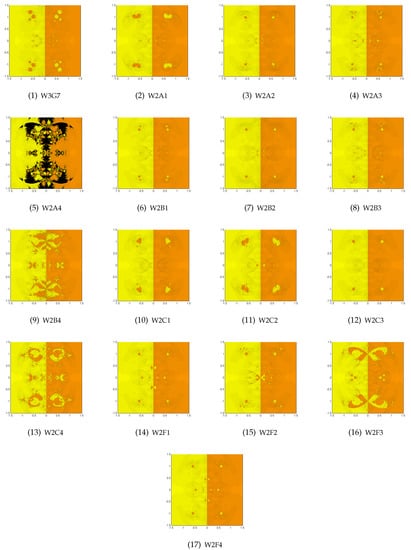
Figure 1. The top row for W3G7 (left), W2A1 (center left), W2A2 (center right) and W2A3 (right). The second row for W2A4 (left), W2B1 (center left), W2B2 (center right) and W2B3 (right). The third row for W2B4 (left), W2C1 (center left), W2C2 (center right) and W2C3 (right). The third row for W2C4 (left), W2F1 (center left), W2F2 (center right), and W2F3 (right). The bottom row for W2F4 (center), for the roots of the polynomial equation ${(z^2-1)}^2$.

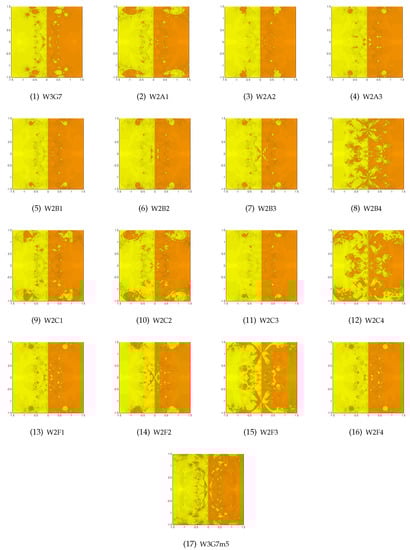
Figure 2. The top row for W3G7 (left), W2A1 (center left), W2A2 (center right) and W2A3 (right). The second row for W2B1 (left), W2B2 (center left), W2B3 (center right) and W2B4 (right). The third row for W2C1 (left), W2C2 (center left), W2C3 (center right) and W2C4 (right). The fourth row for W2F1 (left), W2F2 (center left), W2F3 (center right), and W2F4 (right). The bottom row for W3G7m5 (center), for the roots of the polynomial equation ${(z^2-1)}^k,k\in \{3,5\}$.

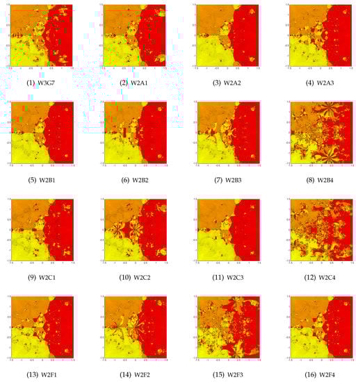
Figure 3. The top row for W3G7 (left), W2A1 (center left), W2A2 (center right) and W2A3 (right). The second row for W2B1 (left), W2B2 (center left), W2B3 (center right) and W2B4 (right). The third row for W2C1 (left), W2C2 (center left), W2C3 (center right) and W2C4 (right). The bottom row for W2F1 (left), W2F2 (center left), W2F3 (center right), and W2F4 (right), for the roots of the polynomial equation ${(3z^3+4z^2-10)}^3$.

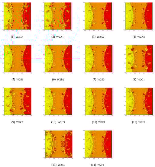
Figure 4. The top row for W3G7 (left), W2A1 (center left), W2A2 (center right) and W2A3 (right). The second row for W2B1 (left), W2B2 (center left), W2B3 (center right) and W2C1 (right). The third row for W2C2 (left), W2C3 (center left), W2F1 (center right) and W2F2 (right). The bottom row for W2F3 (left) and W2F4 (right), for the roots of the polynomial equation ${(z^3-z)}^4$.

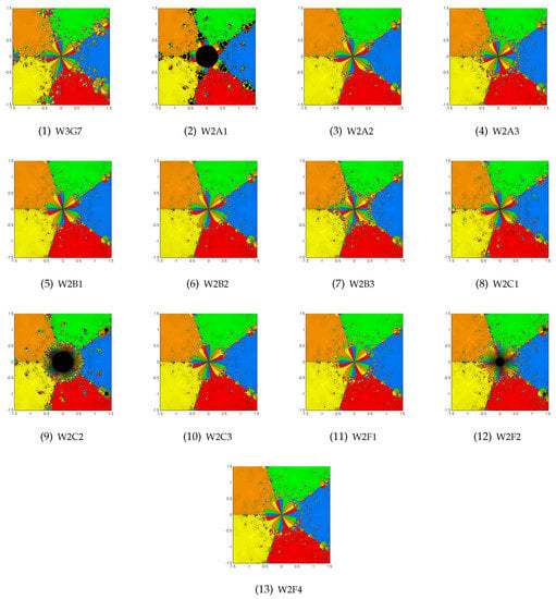
Figure 5. The top row for W3G7 (left), W2A1 (center left), W2A2 (center right) and W2A3 (right). The second row for W2B1 (left), W2B2 (center left), W2B3 (center right) and W2C1 (right). The third row for W2C2 (left), W2C3 (center left), W2F1 (center right) and W2F2 (right). The bottom row for W2F4 (center), for the roots of the polynomial equation ${(z^5-1)}^3$.

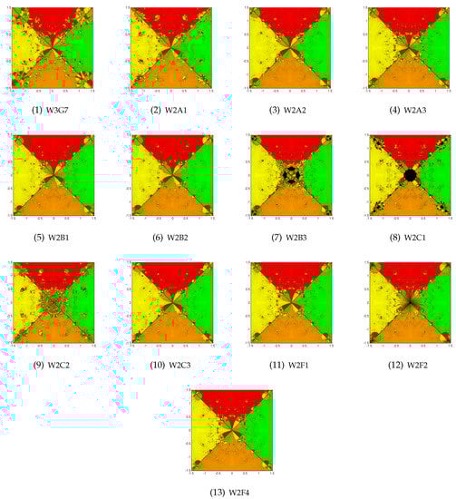
Figure 6. The top row for W3G7 (left), W2A1 (center left), W2A2 (center right) and W2A3 (right). The second row for W2B1 (left), W2B2 (center left), W2B3 (center right) and W2C1 (right). The third row for W2C2 (left), W2C3 (center left), W2F1 (center right) and W2F2 (right). The bottom row for W2F4 (center), for the roots of the polynomial equation ${(z^4-1)}^3$.

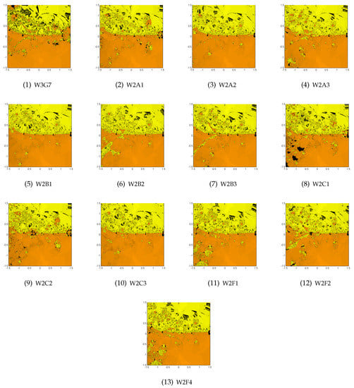
Figure 7. The top row for W3G7 (left), W2A1 (center left), W2A2 (center right) and W2A3 (right). The second row for W2B1 (left), W2B2 (center left), W2B3 (center right) and W2C1 (right). The third row for W2C2 (left), W2C3 (center left), W2F1 (center right) and W2F2 (right). The bottom row for W2F4 (center), for the roots of the non-polynomial equation ${(z+i)}^3{(e^{z-i}-1)}^3$.

Throughout the computational experiments with the aid of Mathematica, $\$MinPrecision=400$ has been assigned to maintain 400 digits of minimum number of precision. If α is not exact, then it is given by an approximate value with 416 digits of precision higher than $\$MinPrecision$.

Limited paper space allows us to list $x_n$ and α with up to 15 significant digits. We set error bound $ϵ=\frac{1}{2}\times {10}^{-360}$ to meet $|x_n-\alpha |<ϵ$. Due to the high-order of convergence and root multiplicity, close initial guesses have been selected to achieve a moderate number of accurate digits of the asymptotic error constants.

Methods W3G7, W2A1, W2C2 and W2F2 successfully located desired zeros of test functions $F_1-F_4$:

$$\left\{\begin{array}{l}\mathbf{W}\mathbf{3}\mathbf{G}\mathbf{7}:F_1\left(x\right)={[cos\left(\frac{\pi x}{2}\right)+2x^2-3\pi ]}^4,\alpha \approx 2.27312045629419,m=4,\hfill \\ \mathbf{W}\mathbf{2}\mathbf{A}\mathbf{1}:F_2\left(x\right)={[cos(x^2+1)-xlog(x^2-\pi +2)+1]}^4·(x^2+1-\pi ),\alpha =\sqrt{\pi -1},m=5,\hfill \\ \mathbf{W}\mathbf{2}\mathbf{C}\mathbf{2}:F_3\left(x\right)={[{sin}^{-1}(x^2-1)+3e^x-2x-3]}^2,\alpha \approx 0.477696831914490,m=2,\hfill \\ \mathbf{W}\mathbf{2}\mathbf{F}\mathbf{2}:F_4\left(x\right)={(x^2+1)}^4+log[1+{(x^2+1)}^3],\alpha =i,m=3,\hfill \\ \mathrm{where}logz(z\in \mathbb{C})\mathrm{is} \mathrm{a} \mathrm{principal} \mathrm{analytic} \mathrm{branch} \mathrm{with}-\pi <Im(logz)\le \pi .\hfill \end{array}\right.$$

(46)

We find that Table 2 ensures sixteenth-order convergence. The computational asymptotic error constant $|e_n|/|e_{n-1}{|}^{16}$ is in agreement with the theoretical one $\eta ={lim}_{n\to \infty }|e_n|/|e_{n-1}{|}^{16}$ up to 4 significant digits. The computational convergence order $p_n=log|e_n/\eta |/log|e_{n-1}|$ well approaches 16.

Additional test functions in Table 3 confirm the convergence of Scheme (1). The errors $|x_n-\alpha |$ are listed in Table 4 for comparison among the listed methods W3G7 and W2A1–W2F4. In the current experiments, W3G7 has slightly better convergence for $f_5$ and slightly poor convergence for all other test functions than the rest of the listed methods. No specific method performs better than the other among methods W2A1–W2F4 of Case 2.

According to the definition of the asymptotic error constant $\eta (c_i,Q_f,K_f,J_f)={lim}_{n\to \infty }|R_f\left(x_n\right)-\alpha |/$$|x_n{-\alpha |}^{16}$, the convergence is dependent on iterative map $R_f\left(x_n\right)$, $f\left(x\right)$, $x_0$, α and the weight functions $Q_f$, $K_f$ and $J_f$. It is clear that no particular method always achieves better convergence than the others for any test functions.

The proposed family of methods (1) has efficiency index $EI$ [38], which is ${16}^{1/5}\approx 1.741101$ and larger than that of Newton’s method. In general, the local convergence of iterative methods (45) is guaranteed with good initial values $x_0$ that are close to α. Selection of good initial values is a difficult task, depending on precision digits, error bound, and the given function $f\left(x\right)$.

The global convergence with appropriate initial values $x_0$ is effectively described by means of a basin of attraction that is the set of initial values leading to long-time behavior approaching the attractors under the iterative action of $R_f$. Basins of attraction contain information about the region of convergence. A method occupying a larger region of convergence is likely to be a more robust method. A quantitative analysis will play the important role for measuring the region of convergence.

The basins of attraction, as well as the relevant statistical data, are constructed in a similar manner shown in the work of Geum–Kim–Neta [19]. Because of the high order, we take a smaller square ${[-1.5,1.5]}^2$ and use $601\times 601$ initial points uniformly distributed in the domain. Maple software has been used to perform the desired dynamics with convergence stopping criteria satisfying $|x_{n+1}-x_n|<{10}^{-6}$ within the maximum number of 40 iterations. An initial point is painted with a color whose intensity measures the number of iterations converging to a root. The brighter color implies the faster convergence. The black point means that its orbit did not converge within 40 iterations.

Despite the limited space, we will explore the dynamics of all listed maps W3G7 and W2A1–W2F4, with applications to $p_k\left(z\right),(1\le k\le 7)$ through the following seven examples. In each example, we have shown dynamical planes for the convergence behavior of iterative map $x_{n+1}=R_f\left(x_n\right)$ (42) with $f\left(z\right)=p_k\left(z\right)$ by illustrating the relevant basins of attraction through Figure 1, Figure 2, Figure 3, Figure 4, Figure 5, Figure 6 and Figure 7 and displaying relevant statistical data in Table 5, Table 6 and Table 7 with colored fonts indicating best results.

Table 5. Average number of iterations per point for each example (1–7).

Map	Example
	1: m = 2	2: m = 3	3: m = 3	4: m = 4	5: m = 3	6: m = 3	7: m = 3	Average
W3G7	2.94	3.48	3.83	3.93	3.95	3.97	6.77	4.12
W2A1	2.84	3.50	3.70	4.04	6.84	3.74	5.49	4.31
W2A2	2.76	3.15	3.52	3.84	3.62	3.66	4.84	3.63
W2A3	2.78	3.21	3.61	3.89	3.70	3.74	4.98	3.70
W2A4	11.40	-	-	-	-	-	-	-
W2B1	2.74	3.25	3.70	3.88	3.67	3.72	5.01	3.71
W2B2	2.95	3.42	3.66	4.01	3.75	3.77	5.15	3.82
W2B3	2.78	3.28	3.64	3.89	3.69	4.65	5.13	3.86
W2B4	3.29	3.91	4.99	-	-	-	-	-
W2C1	2.88	3.66	3.87	4.08	3.89	5.45	6.25	4.30
W2C2	2.93	3.68	3.95	4.15	6.70	4.67	5.75	4.55
W2C3	2.73	3.22	3.53	3.98	3.60	3.62	4.94	3.66
W2C4	3.14	3.81	4.96	-	-	-	-	-
W2F1	2.72	3.24	3.55	3.84	3.49	3.57	5.41	3.69
W2F2	2.81	3.28	3.80	4.06	5.02	4.50	5.29	4.10
W2F3	2.91	3.54	4.36	4.41	-	-	-	-
W2F4	2.71	3.19	3.50	3.86	3.42	3.53	5.52	3.68

Table 6. CPU time (in seconds) required for each example (1–7) using a Dell Multiplex-990.

Map	Example
	1: m = 2	2: m = 3	3: m = 3	4: m = 4	5: m = 3	6: m = 3	7: m = 3	Average
W3G7	1254.077	2983.035	3677.848	3720.670	3944.937	3901.679	4087.102	3367.050
W2A1	1079.667	2694.537	3528.149	3119.911	5896.635	2938.747	3526.840	3254.927
W2A2	969.374	2471.727	3287.081	2956.702	3218.223	2891.478	2981.179	2682.252
W2A3	990.341	2843.789	2859.093	2999.712	3002.146	3074.811	3155.307	2703.600
W2A4	4446.528	-	-	-	-	-	-	-
W2B1	1084.752	2634.826	3295.162	3051.941	2835.755	3238.363	3272.667	2773.352
W2B2	1075.393	2429.996	3130.223	3051.192	2929.106	3581.456	3155.619	2764.712
W2B3	1180.366	2397.111	7193.034	3000.383	2970.711	3739.766	3139.084	3374.351
W2B4	1274.653	2932.008	4872.972	-	-	-	-	-
W2C1	1132.069	2685.355	3242.637	3287.066	3147.663	4080.019	4802.662	3196.782
W2C2	1112.162	2881.697	3189.706	3873.037	5211.619	3665.773	3950.896	3412.127
W2C3	1052.570	2421.026	2768.362	3014.033	2778.518	2914.941	3953.346	2700.399
W2C4	2051.710	4690.295	7193.034	-	-	-	-	-
W2F1	1071.540	2407.158	2909.965	3472.317	2832.230	3490.896	3246.584	2775.813
W2F2	1015.051	2438.483	3031.802	3061.270	3703.152	3737.394	3324.537	2901.670
W2F3	1272.188	2596.200	3603.655	4130.158	-	-	-	-
W2F4	1216.839	2620.052	3589.177	3233.168	3534.312	3521.660	3934.845	3092.865

Table 7. Number of points requiring 40 iterations for each example (1–7).

Map	Example
	1: m = 2	2: m = 3	3: m = 3	4: m = 4	5: m = 3	6: m = 3	7: m = 3	Average
W3G7	677	605	1	250	40	1265	33,072	5130.000
W2A1	657	617	1	166	34,396	1201	18,939	7996.714
W2A2	697	601	1	162	1	1201	15,385	2578.286
W2A3	675	605	55	152	9	1221	14,711	2489.714
W2A4	78,843	-	-	-	-	-	-	-
W2B1	679	613	1	204	9	1201	13,946	2379.000
W2B2	635	609	1	116	1	1217	15,995	2653.429
W2B3	679	613	1	146	3	10,645	16,342	4061.286
W2B4	659	617	2	-	-	-	-	-
W2C1	689	617	1	400	20	18,157	24,239	6303.286
W2C2	669	601	1	174	17,843	1265	18,382	5562.143
W2C3	659	609	1	184	1	1201	14,863	2502.571
W2C4	601	601	1	-	-	-	-	-
W2F1	681	601	1	126	10	1225	18,772	3059.429
W2F2	679	617	101	614	3515	1593	17,469	3512.571
W2F3	663	605	1	78	-	-	-	-
W2F4	645	605	1	130	12	1217	20,020	3232.857

Example 1.

As a first example, we have taken a quadratic polynomial raised to the power of two with all real roots:

$$p_1\left(z\right)={(z^2-1)}^2.$$

(47)

Clearly the roots are $\pm 1$. Basins of attraction for W3G7, W2A1–W2F4 are given in Figure 1. Consulting Table 5, Table 6 and Table 7, we find that the methodsW2B2andW2F4use the least number (2.71) of iterations per point on average (ANIP) followed by W2F1 with 2.72 ANIP, W2C3 with 2.73 and W2B1 with 2.74. The fastest method is W2A2 with 969.374 s followed closely by W2A3 with 990.341 s. The slowest is W2A4 with 4446.528 s. Method W2C4 has the lowest number of black points (601) and W2A4 has the highest number (78843). We will not includeW2A4in the coming examples.

Example 2.

As a second example, we have taken the same quadratic polynomial now raised to the power of three:

$$p_2\left(z\right)={(z^2-1)}^3.$$

(48)

The basins for the best methods are plotted in Figure 2. This is an example to demonstrate the effect of raising the multiplicity from two to three. In one case, namely W3G7, we also have $m=5$ with CPU time of 4128.379 s. Based on the figure we see that W2B4, W2C4 and W2F3 were chaotic. The worst are W2B4, W2C4 and W2F3. In terms of ANIP, the best was W2A2 (3.15) followed by W2F4 (3.19) and the worst was W2B4 (3.91). The fastest was W2B3 using (2397.111 s) followed by W2F1 using 2407.158 s and the slowest was W2C4 (4690.295 s) preceded by W3G7 (2983.035 s). Four methods have the highest number of black points (617). Those were W2A1, W2B4, W2C1 and W2F2. The lowest number was 601 for W2A2, W2C2, W2C4 and W2F1.

Comparing the CPU time for the cases $m=2$ and $m=3$ of W3G7, we find it is about doubled. But when increasing from three to five, we only needed about 50% more.

Example 3.

In our third example, we have taken a cubic polynomial raised to the power of three:

$$p_3\left(z\right)={(3z^3+4z^2-10)}^3.$$

(49)

Basins of attraction are given in Figure 3. It is clear that W2B4, W2C4 and W2F3 were too chaotic and they should be eliminated from further consideration. In terms of ANIP, the best was W2F4 (3.50) followed by W2A2 (3.52), W2C3 (3.53) and W2F1 (3.55) and the worst were W2B4 and W2C4 with 4.99 and 4.96 ANIP, respectively. The fastest was W2C3 using 2768.362 s and the slowest was W2B3 (7193.034 s). There were 13 methods with only one black point and one with two points. The highest number of black points was 101 for W2F2.

Example 4.

As a fourth example, we have taken a different cubic polynomial raised to the power of four:

$$p_4\left(z\right)={(z^3-z)}^4.$$

(50)

The basins are given in Figure 4. We now see that W2F3 is the worst. In terms of ANIP, W2A2 and W2F1 were the best (3.84 each) and the worst was W2F3 (4.41). The fastest was W2A2 (2956.702 s) and the slowest was W2F3 (4130.158 s). The lowest number of black points (78) was for method W2F3 and the highest number (614) for W2F2. We did not include W2F3 in the rest of the experiments.

Example 5.

As a fifth example, we have taken a quintic polynomial raised to the power of three:

$$p_3\left(z\right)={(z^5-1)}^3.$$

(51)

The basins for the best methods left are plotted in Figure 5. The worst were W2A1 and W2C2. In terms of ANIP, the best was W2F4 (3.42) followed by W2F1 (3.49) and the worst were W2A1 (6.84) and W2C2 (6.70). The fastest was W2C3 using 2778.518 s followed by W2F1 using 2832.23 s and W2B1 using 2835.755 s. The slowest was W2A1 using 5896.635 s. There were three methods with one black point (W2A2, W2B2 and W2C3) and four others with 10 or less such points, namely W2B3 (3), W2A3 and W2B1 (9) and W2F1 (10). The highest number was for W2A1 (34,396) preceded by W2C2 with 17,843 black points.

Example 6.

As a sixth example, we have taken a quartic polynomial raised to the power of three:

$$p_6\left(z\right)={(z^4-1)}^3.$$

(52)

The basins for the best methods left are plotted in Figure 6. It seems that most of the methods left were good except W2B3 and W2C1. Based on Table 5 we find that W2F4 has the lowest ANIP (3.53) followed by W2F1 (3.57). The fastest method was W2A2 (2891.478 s) followed by W2C3 (2914.941 s). The slowest was W2C1 (4080.019 s) preceded by W3G7 using 3901.679 s. The lowest number of black points was for W2A1, W2A2, W2B1 and W2C3 (1201) and the highest number was for W2C1 with 18,157 black points.

Example 7.

As a seventh example, we have taken a non-polynomial equation having $\pm i$ as its triple roots:

$$p_6\left(z\right)={(z+i)}^3{(e^{z-i}-1)}^3,withi=\sqrt{-1}.$$

(53)

The basins for the best methods left are plotted in Figure 7. It seems that most of the methods left have a larger basin for the root $-i$, i.e., the boundary does not match the real line exactly. Based on Table 5 we find that W2A2 has the lowest ANIP (4.84) followed by W2C3 (4.94) and W2A3 (4.98). The fastest method was W2A2 (2981.179 seconds) followed by W2B3 (3139.084 s), W2A3 (3155.307 s) and W2B2 (3155.619 s). The slowest was W2C1 (4802.662 s). The lowest number of black points was for W2B1 (13,946) and the highest number was for W3G7 with 33,072 black points. In general all methods had higher number of black points compared to the polynomial examples.

We now average all these results across the seven examples to try and pick the best method. W2A2 had the lowest ANIP (3.63), followed by W2C3 with 3.66, W2F4 with 3.68 and W2F1 with 3.69. The fastest method was W2A2 (2682.252 seconds), followed by W2C3 (2700.399 s) and W2A3 using 2703.600 s of CPU. W2B1 has the lowest number of black points on average (2379), followed by W2A3 (2490 black points). The highest number of black points was for W2A1.

Based on these seven examples we see that W2F4 has four examples with the lowest ANIP, W2A2 had three examples and W2F1 has one example. On average, though, W2A2 had the lowest ANIP. W2A2 was the fastest in four examples and on average. W2C3 was the fastest in two examples and W2B3 in one example. In terms of black points, W2A2, W2B1 and W2B3 had the lowest number in three examples and W2F1 in two examples. On average W2B1 has the lowest number. Thus, we recommend W2A2, since it is in the top in all categories.

5. Conclusions

Both numerical and dynamical aspects of iterative map (1) support the main theorem well through a number of test equations and examples. The W2C2 and W2B3 methods were observed to occupy relatively slower CPU time. Such dynamical aspects would be greatly strengthened if we could include a study of parameter planes with reference to appropriate parameters in Table 1.

The proposed family of methods (1) employing generic weight functions favorably cover most of optimal sixteenth-order multiple-root finders with a number of feasible weight functions. The dynamics behind the purely imaginary extraneous fixed points will choose best members of the family with improved convergence behavior. However, due to the high order of convergence, the algebraic difficulty might arise resolving its increased complexity. The current work is limited to univariate nonlinear equations; its extension to multivariate ones becomes another task.

References

- Bi, W.; Wu, Q.; Ren, H. A new family of eighth-order iterative methods for solving nonlinear equations. Appl. Math. Comput. 2009, 214, 236–245. [Google Scholar] [CrossRef]
- Cordero, A.; Torregrosa, J.R.; Vassileva, M.P. Three-step iterative methods with optimal eighth-order convergence. J. Comput. Appl. Math. 2011, 235, 3189–3194. [Google Scholar] [CrossRef]
- Geum, Y.H.; Kim, Y.I. A uniparametric family of three-step eighth-order multipoint iterative methods for simple roots. Appl. Math. Lett. 2011, 24, 929–935. [Google Scholar] [CrossRef]
- Lee, S.D.; Kim, Y.I.; Neta, B. An optimal family of eighth-order simple-root finders with weight functions dependent on function-to-function ratios and their dynamics underlying extraneous fixed points. J. Comput. Appl. Math. 2017, 317, 31–54. [Google Scholar] [CrossRef]
- Liu, L.; Wang, X. Eighth-order methods with high efficiency index for solving nonlinear equations. Appl. Math. Comput. 2010, 215, 3449–3454. [Google Scholar] [CrossRef]
- Petković, M.S.; Neta, B.; Petković, L.D.; Džunić, J. Multipoint Methods for Solving Nonlinear Equations; Elsevier: New York, NY, USA, 2012. [Google Scholar]
- Petković, M.S.; Neta, B.; Petković, L.D.; Džunić, J. Multipoint methods for solving nonlinear equations: A survey. Appl. Math. Comput. 2014, 226, 635–660. [Google Scholar] [CrossRef]
- Sharma, J.R.; Arora, H. A new family of optimal eighth order methods with dynamics for nonlinear equations. Appl. Math. Comput. 2016, 273, 924–933. [Google Scholar] [CrossRef]
- Rhee, M.S.; Kim, Y.I.; Neta, B. An optimal eighth-order class of three-step weighted Newton’s methods and their dynamics behind the purely imaginary extraneous fixed points. Int. J. Comput. Math. 2017, 95, 2174–2211. [Google Scholar] [CrossRef]
- Kung, H.T.; Traub, J.F. Optimal order of one-point and multipoint iteration. J. Assoc. Comput. Mach. 1974, 21, 643–651. [Google Scholar] [CrossRef]
- Maroju, P.; Behl, R.; Motsa, S.S. Some novel and optimal families of King’s method with eighth and sixteenth-order of convergence. J. Comput. Appl. Math. 2017, 318, 136–148. [Google Scholar] [CrossRef]
- Sharma, J.R.; Argyros, I.K.; Kumar, D. On a general class of optimal order multipoint methods for solving nonlinear equations. J. Math. Anal. Appl. 2017, 449, 994–1014. [Google Scholar] [CrossRef]
- Neta, B. On a family of Multipoint Methods for Non-linear Equations. Int. J. Comput. Math. 1981, 9, 353–361. [Google Scholar] [CrossRef]
- Geum, Y.H.; Kim, Y.I.; Neta, B. Constructing a family of optimal eighth-order modified Newton-type multiple-zero finders along with the dynamics behind their purely imaginary extraneous fixed points. J. Comput. Appl. Math. 2018, 333, 131–156. [Google Scholar] [CrossRef]
- Ahlfors, L.V. Complex Analysis; McGraw-Hill Book, Inc.: New York, NY, USA, 1979. [Google Scholar]
- Hörmander, L. An Introduction to Complex Analysis in Several Variables; North-Holland Publishing Company: Amsterdam, The Netherlands, 1973. [Google Scholar]
- Shabat, B.V. Introduction to Complex Analysis PART II, Functions of several Variables; American Mathematical Society: Providence, RI, USA, 1992. [Google Scholar]
- Wolfram, S. The Mathematica Book, 5th ed.; Wolfram Media: Champaign, IL, USA, 2003. [Google Scholar]
- Geum, Y.H.; Kim, Y.I.; Neta, B. Developing an Optimal Class of Generic Sixteenth-Order Simple-Root Finders and Investigating Their Dynamics. Mathematics 2019, 7, 8. [Google Scholar] [CrossRef]
- Stewart, B.D. Attractor Basins of Various Root-Finding Methods. Master’s Thesis, Naval Postgraduate School, Department of Applied Mathematics, Monterey, CA, USA, June 2001. [Google Scholar]
- Vrscay, E.R.; Gilbert, W.J. Extraneous Fixed Points, Basin Boundaries and Chaotic Dynamics for shröder and König rational iteration Functions. Numer. Math. 1988, 52, 1–16. [Google Scholar] [CrossRef]
- Amat, S.; Busquier, S.; Plaza, S. Review of some iterative root-finding methods from a dynamical point of view. Scientia 2004, 10, 3–35. [Google Scholar]
- Argyros, I.K.; Magreñán, A.Á. On the convergence of an optimal fourth-order family of methods and its dynamics. Appl. Math. Comput. 2015, 252, 336–346. [Google Scholar] [CrossRef]
- Chun, C.; Lee, M.Y.; Neta, B.; Džunić, J. On optimal fourth-order iterative methods free from second derivative and their dynamics. Appl. Math. Comput. 2012, 218, 6427–6438. [Google Scholar] [CrossRef]
- Chicharro, F.; Cordero, A.; Gutiérrez, J.M.; Torregrosa, J.R. Complex dynamics of derivative-free methods for nonlinear equations. Appl. Math. Comput. 2013, 219, 7023–7035. [Google Scholar] [CrossRef]
- Chun, C.; Neta, B. Comparison of several families of optimal eighth order methods. Appl. Math. Comput. 2016, 274, 762–773. [Google Scholar] [CrossRef]
- Cordero, A.; García-Maimó, J.; Torregrosa, J.R.; Vassileva, M.P.; Vindel, P. Chaos in King’s iterative family. Appl. Math. Lett. 2013, 26, 842–848. [Google Scholar] [CrossRef]
- Geum, Y.H.; Kim, Y.I.; Magreñán, Á.A. A biparametric extension of King’s fourth-order methods and their dynamics. Appl. Math. Comput. 2016, 282, 254–275. [Google Scholar] [CrossRef]
- Geum, Y.H.; Kim, Y.I.; Neta, B. A class of two-point sixth-order multiple-zero finders of modified double-Newton type and their dynamics. Appl. Math. Comput. 2015, 270, 387–400. [Google Scholar] [CrossRef]
- Geum, Y.H.; Kim, Y.I.; Neta, B. A sixth-order family of three-point modified Newton-like multiple-root finders and the dynamics behind their extraneous fixed points. Appl. Math. Comput. 2016, 283, 120–140. [Google Scholar] [CrossRef]
- Magreñan, Á.A. Different anomalies in a Jarratt family of iterative root-finding methods. Appl. Math. Comput. 2014, 233, 29–38. [Google Scholar]
- Neta, B.; Scott, M.; Chun, C. Basin attractors for various methods for multiple roots. Appl. Math. Comput. 2012, 218, 5043–5066. [Google Scholar] [CrossRef]
- Neta, B.; Chun, C.; Scott, M. Basins of attraction for optimal eighth order methods to find simple roots of nonlinear equations. Appl. Math. Comput. 2014, 227, 567–592. [Google Scholar] [CrossRef]
- Scott, M.; Neta, B.; Chun, C. Basin attractors for various methods. Appl. Math. Comput. 2011, 218, 2584–2599. [Google Scholar] [CrossRef]
- Chun, C.; Neta, B. Basins of attraction for Zhou-Chen-Song fourth order family of methods for multiple roots. Math. Comput. Simul. 2015, 109, 74–91. [Google Scholar] [CrossRef]
- Neta, B.; Chun, C. Basins of attraction for several optimal fourth order methods for multiple roots. Math. Comput. Simul. 2014, 103, 39–59. [Google Scholar] [CrossRef]
- Beardon, A.F. Iteration of Rational Functions; Springer: New York, NY, USA, 1991. [Google Scholar]
- Traub, J.F. Iterative Methods for the Solution of Equations; Chelsea Publishing Company: Chelsea, VT, USA, 1982. [Google Scholar]
© 2019 by the authors. Licensee MDPI, Basel, Switzerland. This article is an open access article distributed under the terms and conditions of the Creative Commons Attribution (CC BY) license (http://creativecommons.org/licenses/by/4.0/).