Using G-Functions to Investigate the Evolutionary Stability of Bacterial Quorum Sensing

Abstract

In ecology, G-functions can be employed to define a growth function G for a population b, which can then be universally applied to all individuals or groups $b_i$ within this population. We can further define a strategy $v_i$ for every group $b_i$. Examples for strategies include diverse behaviour such as number of offspring, habitat choice, and time of nesting for birds. In this work, we employ G-functions to investigate the evolutionary stability of the bacterial cooperation process known as quorum sensing. We employ the G-function ansatz to model both the population dynamics and the resulting evolutionary pressure in order to find evolutionary stable states. This results in a semi-linear parabolic system of equations, where cost and benefit are taken into account separately. Depending on different biological assumptions, we analyse a variety of typical model functions. These translate into different long-term scenarios for different functional responses, ranging from single-strategy states to coexistence. As a special feature, we distinguish between the production of public goods, available for all subpopulations, and private goods, from which only the producers can benefit.

1. Introduction

Since its discovery in 1977 [1], quorum sensing (QS) has received increasing attention as a mechanism of bacterial communication. Nowadays, we know that QS coordinates a range of behaviours at the population level [2]. One of those is the production of iron-scavenging molecules, so-called siderophores, in Pseudomonas aeruginosa. The bacteria secrete the siderophores and other virulence factors into the surrounding medium, where their benefit can be shared by all cells in the local population, leading to the term public goods [3,4], e.g., with the focus on kin selection in [5] or the conflict between individual and group interests in [6]. However, such a cooperative system is vulnerable to exploitation by non-cooperative cheaters. Gaining all the benefits of QS without incurring the metabolic costs, these cheater mutants have a growth advantage compared to the wild-type. Studies have shown that such mutants arise in laboratory conditions as well as in infection models [7,8,9,10,11,12,13] and act as social cheats. A few examples of these social cheats can be found in [3,14,15] (all considering the Gram-negative P. aeruginosa), while Pollitt et al. [16] provided an example from the Gram-positive S. aereus.

This gives rise to questions about the evolutionary stability of QS. Once cheaters arise (e.g., through loss-of-function mutation), they should theoretically outgrow the producers as they have more resources available to invest in cell division. Cheaters have been shown to outcompete producers both in vitro and in vivo, but QS seems to be evolutionary stable in natural systems nevertheless. In contrast to the aforementioned public goods, private goods are only accessible to the producing cell itself. They are hence innately protected from cheaters and provide their benefit exclusively for cells with a functioning QS system. Apart from extracellular molecules, QS also controls the production of proteins which act within the cell. In P. aeruginosa, one such protein is nucleoside hydrolase (Nuh). As Nuh is involved in metabolising adenosine, only bacteria with intact signal receptors can digest this carbon source. In this way, cooperation via QS provides a private fitness benefit to cooperating cells if adenosine is available as carbon source [17]. Schuster et al. [18] discussed the benefits attained from private goods. Specifically, on the question why public goods are ultimately stable, they suggested that, in fact, the private good is, directly or indirectly, involved in cooperative behaviour.

Extracellular molecules do not provide benefit indiscriminately, but are limited by diffusion and habitat structure. Kümmerli et al. [19] found a negative correlation between habitat structure and water solubility of siderophores, a class of secreted enzymes under QS control in a wide range of bacteria. For highly structured environments such as animal tissues, water solubility of siderophores is high, while microstructures in the environment naturally limit the resulting diffusion. Conversely, water solubility of siderophores is low in unstructured environments such as water habitats. This leads to siderophores clinging to each other as well as to lipid membranes. In this way, a fraction of the siderophores stay with their producer and provide some private benefit.

Several mechanisms, such as kin selection [20] and policing [21], have been described that could explain the evolutionary stability of cooperation and QS despite the advantages cheaters have in such a system.

In addition to experimental approaches, there have been many different mathematical modelling approaches to study QS, from stochastic cellular automata [22] to classic individual-based models [23], including differential equations [24]. In this paper, we develop a mathematical model to investigate the evolutionary stability of QS, which results in a semi-linear parabolic system of equation, following Frank [25] and Mund et al. [26], who used an age-dependent model as basis to check evolutionary stability. We explore the population dynamics between secretors and cheaters and are also interested in the evolutionary pressure that arises through those population dynamics. As such, we employ the G-function ansatz that was introduced by Cohen et al. [27] and further developed since then [28,29,30,31]. With the G-function ansatz, one finds a function G which describes the growth rate of a subpopulation. This function is dependent on the strategy of this subpopulation and both population numbers and strategies of other existing subpopulations (see Figure 1). A strategy can be taken to be any behaviour of interest which can be assigned a real number.

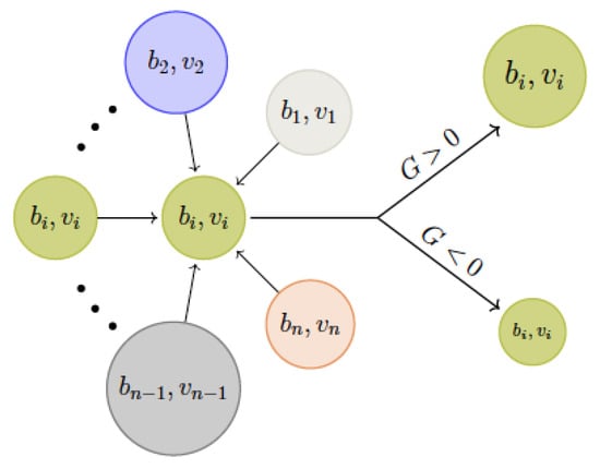
Figure 1. Schematic representation of influences on the growth rate of a population: the growth rate G of a subpopulation will be mainly influenced by three factors: its own strategy $v_i$, the environment defined by the complete strategy set v and the whole population b.

In our case, we take the QS-intensity of the subpopulation as the strategy. A strategy value of zero therefore denotes a QS cheater, while we assume a value of one to be the normal output of QS active secretors. If we take $v_i$ as the strategy of the subpopulation, v is the vector of strategy values for all subpopulations. Accordingly, $b_i$ and b represent the population numbers of subpopulation i and the complete vector, respectively. The population dynamics for subpopulation i thus follows the equation

$$\dot{b_i}\left(t\right)=G(v_i\left(t\right),v\left(t\right),b\left(t\right))·b_i\left(t\right).$$

(1)

At the same time, the per-capita growth function G also governs the evolutionary dynamics of the population. If we calculate the derivative of G with respect to the subpopulation strategy, we find the direction of higher per-capita growth. This is the direction evolutionary forces will drive the population, leading to

$$\dot{v_i}\left(t\right)={\partial }_u{G(u,v\left(t\right),b\left(t\right))|}_{u=v_i\left(t\right)}.$$

(2)

To simplify notation from here on, we define

$$\begin{array}{c}{\partial }_{1}G(v_i,v,b):={\partial }_{u}G(u,v,b){|}_{u=v_i}.\end{array}$$

(3)

This framework allows us to find strategy values which are resistant against others in such a way that, under the influence of natural selection, no other strategy can invade the population. These strategies are called evolutionary stable strategies (ESS) [32].

Many experiments have shown the importance of spatial arrangements when considering bacterial interaction [33,34]. As such, we aim to include spatial variables in our model. This can be done in various ways, but we concentrate on the one that was introduced by Kronik and Cohen [31]. This leads to a system of partial differential equations.

In [35], we showed the existence and uniqueness of weak and classical solutions to the associated semi-linear parabolic system in Equations (1) and (2) with Robin boundary conditions using the coupled upper-lower solution approach. In this paper, we analyse a variety of typical model functions. These translate into different long-term scenarios for different functional responses, ranging from single-strategy states to coexistence. In Section 2, we introduce the basic model and some assumptions we work with, before considering private goods models in Section 3. These models are then analysed numerically in Section 4. In Section 5, we summarise and interpret our findings.

2. The Basic Model: Using the G-Function Approach

In this case G takes the form:

$$\begin{array}{cc}\hfill G(v_i,v,b)& =B(v,b)·C\left(v_i\right)-\mu {||b||}_1.\hfill \end{array}$$

(4)

For a formulation with carrying capacity instead of population-dependent death rate, we can transform this equation into

$$\begin{array}{cc}\hfill G(v_i,v,b)& =B(v,b)C\left(v_i\right)\left(1-\frac{\mu {||b||}_1}{B(v,b)C\left(v_i\right)}\right),\hfill \end{array}$$

(5)

which gives us $B(v,b)C\left(v_i\right)/\mu$ as the capacity for the population. We can now look at the derivative of G with respect to $v_i$.

$$\begin{array}{c}{\partial }_{1}G(v_i,v,b)=B(v,b)·C^{\prime }\left(v_i\right).\end{array}$$

(6)

We make some regularity assumptions on G and its derivative to simplify the mathematical analysis. These do not restrict our biological application, as our model growth functions do not include discontinuous behaviour and are smooth.

(I)

$G(v_i,v,b)$ is Lipschitz continuous in all variables.

(II)

${\partial }_{1}G(v_i,v,b)$ is Lipschitz continuous in ${(v,b)}^T$,

where ${}^T$ denotes transpose. Additionally, we make some assumptions on G from the biological background.

(III)

$G(v_i,v,b)$ has a (direct or indirect) negative feedback loop in $b_i$. The population number cannot go towards infinity.

(IV)

$\exists \overline{u}\forall (v,b){\partial }_{1}G(v_i,v,b)\le 0\forall v_i>\overline{u}$. From a certain threshold onwards, higher strategy values no longer not a higher net growth.

(V)

$\exists \underline{u}<\overline{u}\forall (v,b):{\partial }_{1}G(\underline{u},v,b)=0$. Reducing the strategy further than the value $\underline{u}$ provides no higher growth rate.

These assumptions ensure that Equation (21) does not exhibit divergent behaviour ($v\to \infty$ and/or $b\to \infty$), which is not biologically plausible. If, e.g., ${\partial }_{1}G(v_i,v,b)\ge \gamma >0\forall v_i$, then $c+\lambda t$ with $\lambda =\gamma ·\epsilon$ is a lower solution of Equation (21b), as

$$\epsilon {\partial }_{1}G(\lambda t+c,v,b)-\lambda \ge 0.$$

It follows that $v_i\ge c+\lambda t$ and thus $v_i\to \infty$. This would mean ever-increasing strategy values without some kind of trade-off, which we do not find in nature.

In the special case of QS, we take $\underline{u}$ to be 0, requiring ${\partial }_{1}G(0,v,b)=0$. This keeps v from leaving the biologically meaningful parameter range ${\mathbb{R}}_0^{+}$ (production cannot be lower than 0).

2.1. Cost and Benefit

To model the G-function for QS, one of the avenues we can take is to divide the impact of $v_i$, v, and b into two parts: a growth term influenced by $v_i$ and a benefit provided by v, b, and possibly also $v_i$. This reflects the fact that production of QS molecules is costly to the individual, while the resulting factors are public goods and therefore provide benefit to all bacteria. The additional dependence on $v_i$ can be seen as a form of private benefit and is discussed in detail when it occurs.

One important thing to note is that the growth term is actually reduced with rising $v_i$, as increased public good production incurs increased metabolic costs. In this way, less energy is retained for reproduction. We denote the cost term by $C:\mathbb{R}\to {\mathbb{R}}_{+}$, and make the following assumptions:

(VI)

As public good production is costly, C is strictly monotonically decreasing for $v_i\in [0,\infty )$.

(VII)

When producing public goods, the growth rate is reduced by a certain factor:

$$\begin{array}{ccc}\hfill 0<C\left(v_i\right)<1\mathrm{for}{v}_i\ne 0,& \hfill & \hfill C\left(0\right)=1.\end{array}$$

(7)

While Item (VI) is clear from our assumptions on QS, Item (VII) is not as immediately clear. We introduce Item (VII) because we use this factor multiplicatively for G. Thus, a value of 1 would signify unimpeded growth, while a value between 0 and 1 reduces growth. In this way, we assume that QS costs alone do not lead to negative growth rates.

The benefit of QS is provided by secreting extracellular proteins. We denote it by $B:{\mathbb{R}}^m\times {\mathbb{R}}^m\to {\mathbb{R}}_{+}$ and make two main assumptions here:

(VIII)

There is a limit to how much benefit can be obtained,

$$\begin{array}{c}\underset{v\to \infty }{lim}B(v,b)=B_{\max }.\end{array}$$

(8)

(IX)

There is no benefit if no public goods are produced,

$$\begin{array}{c}B(v,b)=0,\mathrm{if}b=0,\sum _i{b}_i{v}_i=0.\end{array}$$

(9)

Equation (8) models a saturation behaviour for the benefit—even if the cells were producing an infinite amount of extracellular protein, the benefit that can be derived is still capped through saturation of enzymes or similar phenomena. Equation (9) ensures that there is no benefit from QS when there are no living bacteria, or all of them have stopped participating in QS.

2.2. Analysis

We know from Assumption (VI) that $C\left(v_i\right)$ is strictly monotonically decreasing for positive $v_i$. Combined with Assumption (V), we have $C^{\prime }\left(v_i\right)<0\forall v_i>0$, $C^{\prime }\left(0\right)=0$ and there exists only $v_i=0$ as an ESS. As the only stable stationary point, $v_i=0$ will attract all other solutions, leading to the decline of QS.

3. Models with Private Benefit

Following up on the private goods-hypothesis explained in Section 1, we now assume that there is a private benefit associated with producing the public goods, e.g. a small percentage of the produced enzymes may cling to the producing bacteria. We model this by adding a term $B\left(v_i\right)$, which is a benefit term that is solely dependent on the strategy of the subpopulation itself. This $B\left(v_i\right)$ should fulfil similar assumptions to those we made of $B(v,b)$, which is why we choose to denote it by the same letter. Overall, we can write for G:

$$\begin{array}{c}G(v_i,v,b)=(B(v,b)+B\left(v_i\right))·C\left(v_i\right)-\mu {||b||}_1.\end{array}$$

(10)

It follows that

$$\begin{array}{c}\hfill {\partial }_{1}G(v_i,v,b)=\left(B(v,b)+B\left(v_i\right)\right)·C^{\prime }\left(v_i\right)+B^{\prime }\left(v_i\right)·C\left(v_i\right),\end{array}$$

(11)

hence for an ESS it must hold that

$$\begin{array}{c}\hfill -C^{\prime }\left(v_i\right)\left(B(v,b)+B\left(v_i\right)\right)=B^{\prime }\left(v_i\right)C\left(v_i\right).\end{array}$$

(12)

To proceed with a more in-depth analysis, we choose a specific cost function which satisfies all our assumptions,

$$\begin{array}{c}C\left(v_i\right)=exp\left(-K{v}_i^2\right),\end{array}$$

(13)

and look at two specific types of model terms for $B\left(v_i\right)$.

3.1. First Type of Model Terms with Monotonicity Property

The first type of model terms consists of those functions $B\left(v_i\right)$, for which $B^{\prime }\left(v_i\right)/v_i$ is monotonically decreasing in $v_i$. This is the case for all possible concave functions (e.g., those with $B\left(0\right)=0,B(\infty )=\overline{B}>0$), as well as for

$$\begin{array}{ccc}\hfill B\left(v_i\right)=\frac{v_i^2}{v_i^2+a^2},& \hfill & \hfill \mathrm{and}B\left(v_i\right)=-{\mathrm{e}}^{-\omega v_i^2}+1.\end{array}$$

Equation (13) allows us to write Equation (12) as

$$\begin{array}{c}\left(B(v,b)+B\left({\overline{v}}_i\right)\right)\left(2K\right)=\frac{B^{\prime }\left({\overline{v}}_i\right)}{{\overline{v}}_i}=:R\left(v_i\right)\end{array}$$

(14)

for ${\overline{v}}_i\ne 0$. Since we know the left-hand side of this equation to be monotonically increasing, a monotonically decreasing right-hand side means that there can only be one solution to Equation (14). Whether or not a solution exists at all can be determined by looking at the limit behaviour.

We know that $B\left(v_i\right)$ should exhibit a saturation for $v_i\to \infty$, forcing

$$\begin{array}{c}\underset{v_i\to \infty }{lim}\frac{B^{\prime }\left({\overline{v}}_i\right)}{{\overline{v}}_i}=0.\end{array}$$

(15)

We also take a look at the limiting values at 0:

$$\begin{array}{cc}\hfill \underset{v_i\to 0}{lim}\left(B(v,b)+B\left(v_i\right)\right)\left(2K\right)& =2KB(v,b)=:B_0,\hfill \end{array}$$

(16a)

$$\begin{array}{cc}\hfill \underset{v_i\to 0}{lim}\frac{B^{\prime }\left(v_i\right)}{v_i}& =\left\{\begin{array}{cc}{B}^{″}\left(0\right)\hfill & \mathrm{if}{B}^{\prime }\left(0\right)=0\hfill \\ +\infty \hfill & \mathrm{if}{B}^{\prime }\left(0\right)>0\hfill \end{array}\right..\hfill \end{array}$$

(16b)

It follows that for $B^{\prime }\left(0\right)=0$ there exists a positive stationary ${\overline{v}}_i$ if and only if $B^{″}\left(0\right)>2KB(v,b)$, while it always exists if $B^{\prime }\left(0\right)>0$. If such a positive ${\overline{v}}_i$ exists, it is stable (see Appendix B.2.1). If, on the other hand, $B^{\prime }\left(0\right)=0$ but $B^{″}\left(0\right)<2KB(v,b)$, then ${\overline{v}}_i=0$ is an ESS.

3.2. Second Type of Model Terms: Hill Equations

For a second type of model terms, we consider Hill equations. These relatively simple functions are often used in mathematical modelling for cooperative binding of molecules. In the case of QS, Dockery and Keener [36] employed them in the modelling of QS signal regulation. We look at terms of the form

$$\begin{array}{c}B\left(v_i\right)=\frac{v_i^h}{v_i^h+a^h}\end{array}$$

(17)

with $h\ge 3$, as the cases $h=1$ and $h=2$ fall into the first type of model terms. Then, we have

$$\begin{array}{c}R\left(v_i\right)=\frac{B^{\prime }\left(v_i\right)}{v_i}=\frac{h{a}^h{v}_i^{h-2}}{{(v_i^h+a^h)}^2}.\end{array}$$

(18)

Instead of being monotonically decreasing as before, $R\left(v_i\right)$ has the following properties:

• $R\left(0\right)=0$.
• $\underset{v_i\to \infty }{lim}R\left(v_i\right)=0$.
• $R\left(v_i\right)\ge 0\forall v_i\ge 0$, with $R\left(v_i\right)>0$ if $v_i>0$.
• $R\left(v_i\right)$ has exactly one maximum, $R\left(v_i^{\ast }\right)$.
• $R^{\left(n\right)}\left(v_i\right)=\frac{v_i^{h-(n+2)}f\left(v_i\right)}{{(v_i^h+a^h)}^{n+2}}$ for $n\le h-2$, with a function $f\left(v_i\right)$ for which $f\left(0\right)>0$.

For a better understanding of the ideas behind, we assume for a moment that $B(v,b)>0$. If we can now show that $R\left(v_i^{\ast }\right)>2K(B(v,b)+B\left(v_i^{\ast }\right))$, two positive stationary solutions $v_i$ to Equation (12) exist.

$$\begin{array}{cccc}\hfill R\left(v_i^{\ast }\right)& =\frac{h·{\left(\frac{h-2}{h+2}\right)}^{\frac{h-2}{h}}}{a^2·{\left(\frac{2h}{h+2}\right)}^2}\hfill & \hfill B\left(v_i^{\ast }\right)& =\frac{h-2}{2h}\hfill \end{array}$$

In that way, $R\left(v_i^{\ast }\right)>2K(B(v,b)+B\left(v_i^{\ast }\right))$ is equivalent to the condition

$$\begin{array}{c}\left(B(v,b)4h+2(h-2)\right)2K{a}^2<{(h-2)}^{\frac{h-2}{h}}{(h+2)}^{\frac{2}{h}}\\ \Rightarrow K{a}^2<\frac{{(h-2)}^{\frac{h-2}{h}}{(h+2)}^{\frac{2}{h}}}{4\left(B\right(v,b)2h+h-2)},\end{array}$$

(19)

which unfortunately cannot be simplified much further, without assumptions on the parameters K and a. We remind ourselves that K is the cost of cooperation, while a denotes the amount of signalling necessary to gain half of the maximal (private) benefits. Equation (19) thus gives upper limits to these terms, dependent on the steepness of the activation curve h as well as the public benefit $B(v,b)$. A larger public benefit is actually detrimental to the existence of positive stationary strategies $v_i$.

At the same time, there cannot be more than two intersections in $[0,+\infty )$ by Rolle’s theorem (see, e.g., [37], p. 134), since

$$\begin{array}{cc}\hfill \left(2KB\right(v,b)& +B\left(v_i\right){)}^{\prime }-R^{\prime }\left(v_i\right)=2K{B}^{\prime }\left(v_i\right)-R^{\prime }\left(v_i\right)\hfill \\ \hfill & =\frac{a^{h}h{v}_i^{h-3}}{{(v_i^h+a^h)}^3}\left(2K{v}_i^2(v_i^h+a^h)+(h+2)v_i^h-(h-2)a^h\right)\hfill \\ \hfill & =\frac{a^{h}h{v}_i^{h-3}}{{(v_i^h+a^h)}^3}\left(2K{v}_i^{h+2}+(h+2)v_i^h+2K{a}^h{v}_i^2-(h-2)a^h\right),\hfill \end{array}$$

(20)

where the term in parenthesis is strictly monotonically increasing and the equation therefore only has one $\xi \in (0,+\infty )$ for which ${(2KB(v,b)+B\left(\xi \right))}^{\prime }-R^{\prime }\left(\xi \right)=0$. Both ${\overline{v}}_i=0$ and the larger of both positive stationary solutions are stable regardless of parameter values (see Appendix B.2.1).

If $B(v,b)=0$, which occurs if for example the existing subpopulations do not engage in QS, the situation is different. As both $R\left(0\right)=0$ and $2KB(v,b)+B\left(0\right)=0$, there can only be one positive intersection. By using Property 5, we know that $R\left(v_i\right)$ is increasing more quickly than $2KB(v,b)+B\left(v_i\right)$ for small $v_i$. It follows that a positive intersection exists. As we know that for $B(v,b)=0$ there is an intersection at $v_i=0$ and from Equation (20) that there can only be two intersections in $[0,+\infty )$, there can be no other positive intersection. Additionally, one can prove this positive intersection to be stable, while the zero solution is unstable (see Appendix B.2.1).

In biological terms, our results indicate that the surrounding subpopulations have a profound impact on the evolution of cooperativity. If one of the subpopulations is cooperating ($B(v,b)\ne 0$), the others will experience bistable behaviour—they might cooperate themselves or not participate in QS, depending on starting strategy. If, on the other hand, all of the subpopulations do not cooperate at first ($B(v,b)=0$), then the evolutionary pressure will drive them towards the positive ESS, meaning they pick up QS with time.

4. Numerical Simulations

The full set of equations we are working with therefore reads

$$\begin{array}{cc}\hfill \dot{b_i}(x,t)& =G(v_i(x,t),v(x,t),b(x,t))·b_i(x,t)+D△b_i(x,t)\hfill \end{array}$$

(21a)

$$\begin{array}{cc}\hfill \dot{v_i}(x,t)& =\epsilon {\partial }_{1}G(v_i(x,t),v(x,t),b(x,t))+D\left(\frac{2\nabla b_i(x,t)·\nabla v_i(x,t)}{b_i(x,t)}+△v_i(x,t)\right),\hfill \end{array}$$

(21b)

noting that $\dot{b_i}(x,t)=\frac{\partial b_i}{\partial t}$.

We used our own experimental data from [34] to derive values for the parameters in our model, which can be found in Table A1. Our aim here was to obtain rough estimates which replicate the general qualitative behaviour, as opposed to fit the experimental data perfectly. To solve the system numerically, we employed the method of lines [38] and used an explicit Runge–Kutta solver on the discretised system. The simulations were run in Matlab.

We assumed a closed system in which the existing subpopulations are mixed but not completely homogeneous in the beginning. This leads to Neumann boundary conditions and the initial distribution displayed in Figure 2.

Figure 2. Visual representation of initial conditions for numerical simulations. For initial conditions, we used patches. The two subpopulations (dark and light patches) were mixed but not homogeneously distributed.

We also added in a feature of QS that we have neglected before: the costs of QS depend on the signal level, as QS products are only produced when the signal level is high enough. We can achieve this by modifying the cost term from Equation (13) to

$$\begin{array}{c}C(v_i,v,b)=exp\left(-K·{\left(B(v,b)·v_i\right)}^2\right),\end{array}$$

(22)

as $B(v,b)$ is a measure for the level of QS. We have not done so before, since it does not change the analysis qualitatively, but leads to unnecessarily long and obfuscating terms.

4.1. Basic Model

We have seen in our calculations that $v_i=0$ is the only stable strategy in this situation. We should therefore have both $v_i\to 0$ and $b_i\to 0$. However, when looking at the simulation results for 3000 $\mathrm{h}$ as displayed in Figure 3, we notice that this convergence is very slow indeed. A quick calculation of ${\partial }_{1}G$ and G for our parameter values confirms that both are close to zero. Thus, even though QS is theoretically unstable, both cheaters and producers persist alongside each other for a very long time, albeit at different densities.

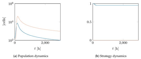
Figure 3. Long-term behaviour of two populations with different start strategies, using a G-function without additions. Both populations numbers are slowly converging in time course towards zero, with producers (dark line) having the lower numbers.

4.2. Models with Private Benefit

In Section 3 we distinguish between two types of model functions. Depending on the Hill coefficient, Hill-terms can fall into either one. We investigated the long-term behaviour for $h=1,2$ or 3.

As predicted, the behaviour in these cases is quite different. For $h\le 2$, $B\left(v_i\right)$ falls into the first type of model functions. For this type, we postulate that there can only be one positive stationary point for v and if it is stable, and then the zero solution is unstable. This is the case for the parameters we calculated. Additionally, we found that for $h=1$ the zero solution is not a stationary point. Thus, both strategies converge towards the stable positive equilibrium, one from above and the other from below. Population 2, which started out as cheaters, gains QS functionality, while there is reduced production from Population 1. Since reducing production is slower to reach the stable point in this parameter constellation, Population 1 succumbs to the population pressure from Population 2 and dies out (see Figure 4). This happens on a rather short time frame of less than 200 $\mathrm{h}$.

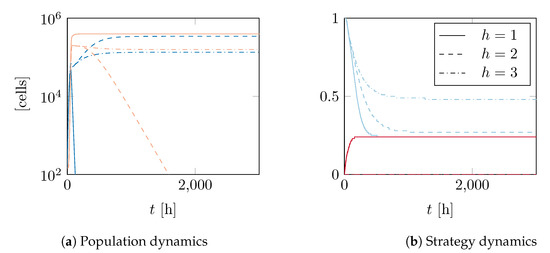
Figure 4. Evolution of two populations with different start strategies, using a G-function with private benefit and hill factors of $h=1$ (line), 2 (dashed) and 3 (dash-dotted). For $h=1$, Population 1 (dark colour) dies out rather quickly, while Population 2 (light colour) gains the QS functionality, albeit at a low level, and remains at a stable population level. If $h=2$, Population 1 reduces its QS strategy to a lower, but stable value. Population 2 is unable to compete and dies out. For $h=3$, Populations 1 and 2 coexistt in a stable way with similar numbers. One population is QS active while the other is not.

For $h=2$, we can see in Figure 4 that once again the strategies converge to a positive value. However, this time the zero solution is a stationary point, although an unstable one. Hence, Population 2 cannot gain QS functionality by starting out with $v_2=0$. The end result is the extinction of Population 2, while Population 1 remains stable.

Overall, for $h\le 2$, we found that one population is driven to extinction, while the other stays at a stable level with QS intact at lower levels.

When $h>2$, $B\left(v_i\right)$ falls into the second type of model functions. That means there might be a stable positive strategy in addition to a stable zero solution. We found this to be the case for $h=3$ for our parameters, as one can see in Figure 4. This means that Populations 1 and 2 remain at stable population and strategy levels, with Population 1 being QS active while Population 2 consists of cheaters. In this scenario, producers and non-producers can live side-by-side indefinitely.

5. Discussion

We have applied the G-function ansatz to the QS dynamics of P. aeruginosa and analysed the resulting model both analytically and numerically. We have found that the type of G-function considered changes the expected outcome drastically.

If we assume that there is no private benefit to QS at all, then the long-term outcome is preassigned and independent of parameters. Whether QS is inactive in all bacteria after some time, or the subpopulation of secretors dies out, the effect remains the same: QS is evolutionary unstable.

As soon as we assume that there is some kind of private benefit, the situation changes. Depending on parameter values, QS might still be unstable, but there can also be positive evolutionary stable secretion values. For the first type of model functions, there is only one stable secretion value. It follows that in the long term the population will unitise (Figure 4). The situation remains much the same if, instead of a direct benefit, we consider a reduction in death rate (results not shown). In contrast, private benefit functions of the second type admit bistable behaviour. This allows secretors and cheaters to coexist indefinitely in addition to single subpopulation states. We have also found that bacteria are driven towards QS if there is no pre-existing cooperation in their environment.

Since the left-hand-side of Equation (12) has a value of zero for $v_i=0$, whereas the right-hand-side has a value greater than zero for $v_i=0$, there could be any number of stable strategies (or none) if one chooses different functional responses.

Our model functions have simplified the actual process of QS a great deal, but one could also include direct dependencies on the signal molecules and enzymes produced. Such models with abiotic components were considered by Cohen et al. [30]. While their short-term dynamics might differ from the scenarios we have considered, their long-term outcome does not. They are also difficult to analyse without resorting to numerical methods, which is why we have concentrated on the simplified functions.

The G-function has allowed us to determine the long-term evolution of QS by considering the short-term population dynamics. By analysing different functional responses, we have explored some possible outcomes. One could also further refine the population dynamics for different real world scenarios. The G-function serves to always model the resulting evolutionary pressure, which tells us something about the way mutation and selection are going to drive the population. As both are happening on a fast time-scale in bacteria, they have a big impact on the interaction between bacterial populations as well as on their interaction with humans (see, e.g., [3]). The G-function can thus be a valuable tool in modelling bacterial interactions.

For completeness, in Appendix C, we show the spatial evolution of two populations with different start strategies, using a G-function without additions (Figure A1) and with private benefit and a hill factor of $h=1$ (Figure A2).

Lastly, we would like to refer the interested reader to the following associated publications which complement this study: Mund et al. [34] and Mund et al. [35].

Appendix B.1. Properties of R(V_i) for the Second Type of Model Terms

We first prove that $R\left(v_i\right)$ has exactly one maximum as well as calculate its maximal value. To that end, we take the derivative of R

$$\begin{array}{cc}\hfill R^{\prime }\left(v_i\right)& =\frac{a^{h}h{v}_i^{h-3}\left(-(h+2)v_i^h+(h-2)a^h\right)}{{\left(v_i^h+a^h\right)}^3}\hfill \end{array}$$

(A1)

and search for critical points

$$\begin{array}{cc}\hfill 0& =a^{h}h{v}_i^{h-3}\left(-(h+2)v_i^h+(h-2)a^h\right).\hfill \end{array}$$

(A2)

For $h>3$, there exists a critical point at $v_i=0$. However, since $R\left(0\right)=0$ and $R\left(v_i\right)>0$ for $v_i>0$, this critical point is clearly a minimum on the bounded space $v_i\in {\mathbb{R}}_0^{+}$. The other critical point satisfies

$$\begin{array}{c}{v}_i^{\ast }=\sqrt[h]{\frac{h-2}{h+2}}·a\end{array}$$

and is thus unique in ${\mathbb{R}}_0^{+}$. It remains to show that $v_i^{\ast }$ is indeed a maximum. However, knowing that $R\left(0\right)=0$ and ${lim}_{v_i\to \infty }R\left(v_i\right)=0$, we can conclude that it can only be a maximum.

We prove Property 5 by induction.

base case

We can derive from the definition of $R\left(v_i\right)$ that

$$\begin{array}{cc}\hfill R^{\prime }\left(v_i\right)& =\frac{a^{h}h{v}_i^{h-3}\left(-(h+2)v_i^h+(h-2)a^h\right)}{{\left(v_i^h+a^h\right)}^3}\hfill \\ \hfill & =\frac{v_i^{h-(1+2)}f\left(v_i\right)}{{\left(v_i^h+a^h\right)}^{1+2}},\hfill \end{array}$$

where $f\left(v_i\right)=a^{h}h\left(-(h+2)v_i^h+(h-2)a^h\right)$ and thus $f\left(0\right)=h{a}^{2h}(h-2)>0$.

inductive step

Assuming that the statement holds for $R^{\left(n\right)}\left(v_i\right)$ and that $n+1\le h-2$, we have

$$\begin{array}{cc}\hfill R^{(n+1)}\left(v_i\right)& =({(v_i^h+a^h)}^{n+2}(h-(2+n))v_i^{h-(n+3)}f\left(v_i\right)\hfill \\ \hfill & +{(v_i^h+a^h)}^{n+2}{f}^{\prime }\left(v_i\right)v_i^{h-(n+2)}\hfill \\ \hfill & -(n+2)h{(v_i^h+a^h)}^{n+1}f\left(v_i\right)v_i^{2h-(n+3)})/{\left(v_i^h+a^h\right)}^{2n+4}\hfill \\ \hfill & =\frac{v_i^{h-(n+1+2)}g\left(v_i\right)}{{(v_i^h+a^h)}^{n+1+2}},\hfill \end{array}$$

where

$$\begin{array}{c}g\left(v_i\right)=(v_i^h+a^h)\left((h-(2+n))f\left(v_i\right)+f^{\prime }\left(v_i\right)v_i\right)-(n+2)hf\left(v_i\right)v_i^h.\end{array}$$

and thus $g\left(0\right)=a^h(h-(2+n))f\left(0\right)>0$ since $n<h-2$ and $f\left(0\right)>0$.

It follows that $R^{\left(n\right)}\left(0\right)=0$ for $n<h-2$ and $R^{(h-2)}\left(0\right)>0$. At the same time, a similar argument shows that

$$\begin{array}{c}{\left(2K(B(v,b)+B\left(v_i\right))\right)}^{\left(n\right)}=2K{B}^{\left(n\right)}\left(v_i\right)=\frac{v_i^{h-n}2Kf\left(v_i\right)}{{(v_i^h+a^h)}^{1+n}}.\end{array}$$

As such, ${\left(2K(B(v,b)+B\left(v_i\right))\right)}^{\left(n\right)}=0$ for $n<h$.

Appendix B.2. Stability of ${\overline{v}}_i$

Appendix B.2.1. Models with Private Benefit

First Type of Model Terms

For $B\left(v_i\right)$ in the first type of model terms, we assume that $B^{\prime }\left(v_i\right)/v_i$ is monotonically decreasing. It follows that

$$\begin{array}{cc}\hfill 0& >{\left(\frac{B^{\prime }\left(v_i\right)}{v_i}\right)}^{\prime }=\frac{v_i{B}^{″}\left(v_i\right)-B^{\prime }\left(v_i\right)}{v_i^2}\hfill \\ \hfill \Rightarrow 0& >B^{″}\left(v_i\right)-\frac{B^{\prime }\left(v_i\right)}{v_i}\forall v_i>0.\hfill \end{array}$$

(A3)

Looking at the second derivative of G, we have

$$\begin{array}{cc}\hfill {\partial }_1^{2}G(v_i,v,b)& =\left(B(v,b)+B\left(v_i\right)\right)C^{″}\left(v_i\right)+2B^{\prime }\left(v_i\right)C^{\prime }\left(v_i\right)+B^{″}\left(v_i\right)C\left(v_i\right)\hfill \\ \hfill & =\left((B(v,b)+B\left(v_i\right))\left(-2K+4K^2{v}_i^2\right)+2B^{\prime }\left(v_i\right)(-2K)v_i+B^{″}\left(v_i\right)\right){\mathrm{e}}^{-K{v}_i^2}\hfill \\ \hfill {\partial }_1^{2}G(0,v,b)& =B(v,b)(-2K)+B^{″}\left(0\right),\hfill \end{array}$$

from which we can gather that ${\overline{v}}_i=0$ is stable if $B^{″}\left(0\right)<2KB(v,b)$. We use Equation (14) and substitute for $B(v,b)+B\left({\overline{v}}_i\right)$

$$\begin{array}{cc}\hfill {\partial }_1^{2}G({\overline{v}}_i,v,b)& =\left(\frac{B^{\prime }\left({\overline{v}}_i\right)}{2K{\overline{v}}_i}\left(-2K+4K^2{\overline{v}}_i^2\right)+2B^{\prime }\left({\overline{v}}_i\right)(-2K){\overline{v}}_i+B^{″}\left({\overline{v}}_i\right)\right){\mathrm{e}}^{-K{\overline{v}}_i^2}\hfill \\ \hfill & =\left(-\frac{B^{\prime }\left({\overline{v}}_i\right)}{{\overline{v}}_i}+B^{″}\left({\overline{v}}_i\right)-2K{\overline{v}}_i{B}^{\prime }\left({\overline{v}}_i\right)\right){\mathrm{e}}^{-K{\overline{v}}_i^2}.\hfill \end{array}$$

(A4)

As $B^{\prime }\left(v_i\right)>0$, stability of positive ${\overline{v}}_i$ immediately follows from Equation (A3).

Second Type of Model Terms

We start out by assuming $B(v,b)>0$. We know that $v_i=0$ is stable if $B^{″}\left(0\right)<2KB(v,b)$ and that for $h\ge 3$ it holds that $B^{\prime \prime }\left(0\right)=0$. Hence, $v_i=0$ is an ESS regardless of parameter values.

A positive stationary solution ${\overline{v}}_i$ is stable, if

$$\begin{array}{cc}\hfill 0& >-\left(\frac{1}{{\overline{v}}_i}+2K{\overline{v}}_i\right)B^{\prime }\left({\overline{v}}_i\right)+B^{″}\left({\overline{v}}_i\right)\hfill \\ \hfill \Rightarrow 0& >-\left(\frac{1}{{\overline{v}}_i}+2K{\overline{v}}_i\right)\frac{h{a}^h{\overline{v}}_i^{h-1}}{{({\overline{v}}_i^h+a^h)}^2}+\frac{h{a}^h{\overline{v}}_i^{h-2}\left(-(h+1){\overline{v}}_i^h+(h-1)a^h\right)}{{({\overline{v}}_i^h+a^h)}^3}\hfill \\ \hfill \Rightarrow 0& >-\left(\frac{1}{{\overline{v}}_i}+2K{\overline{v}}_i\right){\overline{v}}_i({\overline{v}}_i^h+a^h)-(h+1){\overline{v}}_i^h+(h-1)a^h.\hfill \end{array}$$

We can rearrange this inequality to

$$\begin{array}{c}\left(\frac{1}{{\overline{v}}_i}+2K{\overline{v}}_i\right){\overline{v}}_i({\overline{v}}_i^h+a^h)+(h+1){\overline{v}}_i^h>(h-1)a^h.\end{array}$$

The larger of both positive stationary solutions fulfils ${\overline{v}}_i>v_i^{\ast }=\sqrt[h]{\frac{h-2}{h+2}}·a$, if it exists. It follows that

$$\begin{array}{cc}\hfill \left(\frac{1}{{\overline{v}}_i}+2K{\overline{v}}_i\right){\overline{v}}_i({\overline{v}}_i^h+a^h)& +(h+1){\overline{v}}_i^h\hfill \\ \hfill & >\left(1+2K{\overline{v}}_i^2\right)\left(\frac{h-2}{h+2}·a^h+a^h\right)+(h+1)·\frac{h-2}{h+2}·a^h\hfill \\ \hfill & >\frac{2h}{h+2}·a^h+\frac{(h+1)(h-2)}{h+2}·a^h\hfill \\ \hfill & =\frac{2h+h^2-h-2}{h+2}·a^h\hfill \\ \hfill & =(h-1)·a^h.\hfill \end{array}$$

Hence, the larger of both positive solutions is always stable, if it exists. It follows immediately from the stability of the zero solution that the smaller of both positive solutions must be unstable.

In the other case, we first note that both $B^{″}\left(0\right)=0$ and $B(v,b)=0$, which means we cannot gain insight into the stability of the zero solution directly through Equation (A4). However, we know that, for small enough $\epsilon >0$, $R\left(\epsilon \right)>2KB\left(\epsilon \right)$ and that there exists only one positive $\xi$ for which $2K{B}^{\prime }\left(\xi \right)=R^{\prime }\left(\xi \right)$. Additionally, we know that $\xi$ lies in the open interval between zero and the positive intersection ${\overline{v}}_i$ and as such is unequal to ${\overline{v}}_i$. It can thus follow that

$$\begin{array}{c}{R}^{\prime }\left({\overline{v}}_i\right)<2K{B}^{\prime }\left({\overline{v}}_i\right)\\ R^{\prime }\left({\overline{v}}_i\right)={\left(\frac{B^{\prime }\left({\overline{v}}_i\right)}{{\overline{v}}_i}\right)}^{\prime }=\frac{B^{″}\left({\overline{v}}_i\right)}{{\overline{v}}_i}-\frac{B^{\prime }\left({\overline{v}}_i\right)}{{\overline{v}}_i^2}\\ \Rightarrow \frac{B^{″}\left({\overline{v}}_i\right)}{{\overline{v}}_i}-\frac{B^{\prime }\left({\overline{v}}_i\right)}{{\overline{v}}_i^2}<2K{B}^{\prime }\left({\overline{v}}_i\right)\\ -2K{B}^{\prime }\left({\overline{v}}_i\right){\overline{v}}_i-\frac{B^{\prime }\left({\overline{v}}_i\right)}{{\overline{v}}_i}+B^{″}\left({\overline{v}}_i\right)<0,\end{array}$$

which is exactly the condition for stability from Equation (A4). For $B(v,b)=0$, we thus have an unstable zero solution and a stable positive strategy.

References

- Hastings, J.; Nealson, K. Bacterial bioluminescence. Annu. Rev. Microbiol. 1977, 31, 549–595. [Google Scholar] [CrossRef] [PubMed]
- Rutherford, S.T.; Bassler, B.L. Bacterial quorum sensing: Its role in virulence and possibilities for its control. Cold Spring Harbor Perspect. Med. 2012, 2, a012427. [Google Scholar] [CrossRef] [PubMed]
- Rumbaugh, K.P.; Diggle, S.P.; Watters, C.M.; Ross-Gillespie, A.; Griffin, A.S.; West, S.A. Quorum sensing and the social evolution of bacterial virulence. Curr. Biol. 2009, 19, 341–345. [Google Scholar] [CrossRef] [PubMed]
- West, S.A.; Griffin, A.S.; Gardner, A.; Diggle, S.P. Social evolution theory for microorganisms. Nat. Rev. Microbiol. 2006, 4, 597–609. [Google Scholar] [CrossRef] [PubMed]
- Diggle, S.P.; Griffin, A.S.; Campbell, G.S.; West, S.A. Cooperation and conflict in quorum-sensing bacterial populations. Nature 2007, 450, 411–414. [Google Scholar] [CrossRef] [PubMed]
- Brown, S.P.; Johnstone, R.A. Cooperation in the dark: Signalling and collective action in quorum-sensing bacteria. Proc. R. Soc. B 2001, 268, 961–965. [Google Scholar] [CrossRef] [PubMed]
- Bjarnsholt, T.; Jensen, P.; Jakobsen, T.H.; Phipps, R.; Nielsen, A.K.; Rybtke, M.T.; Tolker-Nielsen, T.; Givskov, M.; Høiby, N.; Ciofu, O.; et al. Quorum sensing and virulence of Pseudomonas aeruginosa during lung infection of cystic fibrosis patients. PLoS ONE 2010, 5, e10115. [Google Scholar] [CrossRef]
- Dénervaud, V.; TuQuoc, P.; Blanc, D.; Favre-Bonté, S.; Krishnapillai, V.; Reimmann, C.; Haas, D.; Delden, C.V. Characterization of cell-to-cell signaling-deficient Pseudomonas Aeruginosa Strains Colon. Intubated Patients. J. Clin. Microbiol. 2004, 42, 554–562. [Google Scholar] [CrossRef]
- Köhler, T.; Buckling, A.; van Delden, C. Cooperation and virulence of clinical Pseudomonas Aeruginosa Popul. Proc. Natl. Acad. Sci. USA 2009, 106, 6339–6344. [Google Scholar] [CrossRef]
- Schaber, J.A.; Carty, N.L.; McDonald, N.A.; Graham, E.D.; Cheluvappa, R.; Griswold, J.A.; Hamood, A.N. Analysis of quorum sensing-deficient clinical isolates of Pseudomonas Aeruginosa. J. Med. Microbiol. 2004, 53, 841–853. [Google Scholar] [CrossRef]
- Smith, E.E.; Buckley, D.G.; Wu, Z.; Saenphimmachak, C.; Hoffman, L.R.; D’Argenio, D.A.; Miller, S.I.; Ramsey, B.W.; Speert, D.P.; Moskowitz, S.M.; et al. Genetic adaptation by Pseudomonas Aeruginosa Airways Cyst. Fibros. Patients. Proc. Natl. Acad. Sci. USA 2006, 103, 8487–8492. [Google Scholar] [CrossRef] [PubMed]
- West, S.A.; Winzer, K.; Gardner, A.; Diggle, S.P. Quorum sensing and the confusion about diffusion. Trends Microbiol. 2012, 20, 586–594. [Google Scholar] [CrossRef] [PubMed]
- Wilder, C.N.; Allada, G.; Schuster, M. Instantaneous within-patient diversity of Pseudomonas Aeruginosa quorum-sensing populations from cystic fibrosis lung infections Lung Infect. Infec. Immun. 2009, 77, 5631–5639. [Google Scholar] [CrossRef] [PubMed]
- Popat, R.; Crusz, S.A.; Messina, M.; Williams, P.; West, S.A.; Diggle, S.P. Quorum-sensing and cheating in bacterial biofilms. Proc. R. Soc. Lond. B Biol. Sci. 2012, 479. [Google Scholar] [CrossRef]
- Wilder, C.N.; Diggle, S.P.; Schuster, M. Cooperation and cheating in Pseudomonas Aeruginosa: The roles of the las, rhl and pqs quorum-sensing systems. ISME J. 2011, 5, 1332–1343. [Google Scholar] [CrossRef]
- Pollitt, E.J.; West, S.A.; Crusz, S.A.; Burton-Chellew, M.N.; Diggle, S.P. Cooperation, quorum sensing, and evolution of virulence in Staphylococcus Aureus. Infection Immun. 2014, 82, 1045–1051. [Google Scholar] [CrossRef]
- Dandekar, A.A.; Chugani, S.; Greenberg, E.P. Bacterial quorum sensing and metabolic incentives to cooperate. Science 2012, 338, 264–266. [Google Scholar] [CrossRef]
- Schuster, M.; Sexton, D.J.; Hense, B.A. Why quorum sensing controls private goods. Front. Microbiol. 2017, 8, 885. [Google Scholar] [CrossRef]
- Kümmerli, R.; Schiessl, K.T.; Waldvogel, T.; McNeill, K.; Ackermann, M. Habitat structure and the evolution of diffusible siderophores in bacteria. Ecol. Lett. 2014, 17, 1536–1544. [Google Scholar] [CrossRef]
- Buckling, A.; Brockhurst, M.A. Kin selection and the evolution of virulence. Heredity 2008, 100, 484–488. [Google Scholar] [CrossRef]
- Wang, M.; Schaefer, A.L.; Dandekar, A.A.; Greenberg, E.P. Quorum sensing and policing of Pseudomonas Aeruginosa Soc. Cheaters. Proc. Natl. Acad. Sci. USA 2015, 112, 2187–2191. [Google Scholar] [CrossRef] [PubMed]
- Czárán, T.; Hoekstra, R.F. Microbial communication, cooperation and cheating: Quorum sensing drives the evolution of cooperation in bacteria. PLoS ONE 2009, 4, e6655. [Google Scholar] [CrossRef] [PubMed]
- Cremer, J.; Melbinger, A.; Frey, E. Growth dynamics and the evolution of cooperation in microbial populations. Sci. Rep. 2012, 2, 281. [Google Scholar] [CrossRef] [PubMed]
- Pérez-Velázquez, J.; Hense, B.A. Differential Equations Models to Study Quorum Sensing; Springer: New York, NY, USA, 2018; pp. 253–271. ISBN 978-1-4939-7309-5. [Google Scholar] [CrossRef]
- Frank, S.A. Microbial secretor–cheater dynamics. Philos. Trans. R. Soc. Lond. B Biol. Sci. 2010, 365, 2515–2522. [Google Scholar] [CrossRef] [PubMed]
- Mund, A.; Kuttler, C.; Pérez-Velázquez, J.; Hense, B. An age-dependent model to analyse the evolutionary stability of bacterial quorum sensing. J. Theor. Biol. 2016, 405. [Google Scholar] [CrossRef] [PubMed][Green Version]
- Cohen, Y.; Vincent, T.; Brown, J. A G-function approach to fitness minima, fitness maxima, evolutionary stable strategies and adaptive landscapes. Evol. Ecol. Res. 1999, 1, 923–942. [Google Scholar]
- Apaloo, J.; Brown, J.S.; Vincent, T.L. Evolutionary game theory: ESS, convergence stability, and NIS. Evol. Ecol. Res. 2009, 11, 489–515. [Google Scholar]
- Brown, J.S.; Vincent, T.L. G-functions for the hermeneutic circle of evolution. Comput. Oper. Res. 2006, 33, 479–499. [Google Scholar] [CrossRef]
- Cohen, Y.; Pastor, J.; Vincent, T.L. Evolutionary strategies and nutrient cycling in ecosystems. Evol. Ecol. Res. 2000, 2, 719–743. [Google Scholar]
- Kronik, N.; Cohen, Y. Evolutionary games in space. Math. Model. Nat. Phenom. 2009, 4, 54–90. [Google Scholar] [CrossRef][Green Version]
- Müller, J.; Kuttler, C. Methods and Models in Mathematical Biology; Springer: Berlin, Germany, 2015; ISBN 978-3-642-27251-6. [Google Scholar]
- Kümmerli, R.; Griffin, A.S.; West, S.A.; Buckling, A.; Harrison, F. Viscous medium promotes cooperation in the pathogenic bacterium Pseudomonas Aeruginosa. Proc. R. Soc. Lond. B Biol. Sci. 2009, 276, 3531–3538. [Google Scholar] [CrossRef] [PubMed]
- Mund, A.; Diggle, S.P.; Harrison, F. The fitness of Pseudomonas aeruginosa quorum sensing signal cheats is influenced by the diffusivity of the environment. mBio 2017, 8. [Google Scholar] [CrossRef] [PubMed]
- Mund, A.; Kuttler, C.; Perez-Velazquez, J. Existence and uniqueness of solutions to a family of semi-linear parabolic systems using coupled upper-lower solutions. Discret. Contin. Dyn. Syst. B 2019, 24, 5695. [Google Scholar] [CrossRef]
- Dockery, J.D.; Keener, J.P. A mathematical model for quorum sensing in Pseudomonas Aeruginosa. Bull. Math. Biol. 2001, 63, 95–116. [Google Scholar] [CrossRef] [PubMed]
- Königsberger, K. Analysis 1; Springer: Berlin/Heidelberg, Germany, 1992; ISBN 978-3-540-55116-4. [Google Scholar]
- Schiesser, W. The Numerical Method of Lines: Integration of Partial Differential Equation; Elsevier Science: Amsterdam, The Netherlands, 2012; ISBN 9780128015513. [Google Scholar]
© 2019 by the authors. Licensee MDPI, Basel, Switzerland. This article is an open access article distributed under the terms and conditions of the Creative Commons Attribution (CC BY) license (http://creativecommons.org/licenses/by/4.0/).