Different Estimation Methods for Type I Half-Logistic Topp–Leone Distribution

Abstract

In this study, we propose a new flexible two-parameter continuous distribution with support on the unit interval. It can be identified as a special member of the so-called type I half-logistic-G family of distributions, defined with the Topp–Leone distribution as baseline. Among its features, the corresponding probability density function can be left skewed, right-skewed, approximately symmetric, J-shaped, as well as reverse J-shaped, making it suitable for modeling a wide variety of data sets. It thus provides an alternative to the so-called beta and Kumaraswamy distributions. The mathematical properties of the new distribution are determined, deriving the asymptotes, shapes, quantile function, skewness, kurtosis, some power series expansions, ordinary moments, incomplete moments, moment-generating function, stress strength parameter, and order statistics. Then, a statistical treatment of the related model is proposed. The estimation of the unknown parameters is performed by a simulation study exploring seven methods, all described in detail. Two practical data sets are analyzed, showing the usefulness of the new proposed model.

1. Introduction

Over the past several decades, motivated by the growing demand of statistical models in many applied areas, numerous general families of continuous distributions have been introduced. Most of them consist of adding extra parameters to well-established continuous distributions in order to give them new interesting features. The most notorious of these families are the exponentiated-G family [1], the beta-G family [2], and the gamma-G family [3]. Recent promising families include the Kumaraswamy-G family [4], the type I half-logistic-G family [5], the generalized odd log-logistic family [6], the odd power Cauchy family [7], the exponentiated generalized Topp–Leone-G family [8], and the type II general inverse exponential-G family [9].

The foundation of our study is the type I half-logistic-G (TIHL-G) family [5]. This general family is characterized by the cumulative distribution function (cdf) given by

$$\begin{array}{c}\hfill F(x;\lambda ,\zeta )=\frac{1-{[1-G(x;\zeta )]}^{\lambda }}{1+{[1-G(x;\zeta )]}^{\lambda }},x\in \mathbb{R},\end{array}$$

where $\lambda >0$ and $G(x;\zeta )$ is a baseline cdf of a continuous distribution which may depend on a parameter vector $\zeta$. The corresponding probability density function (pdf) is given by

$$f(x;\lambda ,\zeta )=\frac{2\lambda g(x;\zeta ){[1-G(x;\zeta )]}^{\lambda -1}}{{\left\{1+{[1-G(x;\zeta )]}^{\lambda }\right\}}^2},x\in \mathbb{R},$$

where $g(x;\zeta )$ denotes the pdf associated to $G(x;\zeta )$. Also, the corresponding hazard rate function (hrf) is given by

$$h(x;\lambda ,\zeta )=\frac{\lambda g(x;\zeta )}{[1-G(x;\zeta )]\left\{1+{[1-G(x;\zeta )]}^{\lambda }\right\}},x\in \mathbb{R}.$$

In a former work, Cordeiro et al. [5] studied the main mathematical and statistical properties of the type I half-logistic-G family, with an emphasis on special members with support on the semi-infinite interval $(0,+\infty )$. In particular, it is shown that the additional parameter $\lambda$ plays a significant role, allowing new features to be reached in terms of flexibility in comparison to the baseline distribution. Applications to two practical data sets are given for the type I half-logistic-G family defined with the Weibull distribution as baseline. Numerical results show great adjustments of the proposed model for both data sets, with the use of the maximum likelihood method to estimate the model parameters.

In this study, we investigate the potential of a new special member of the type I half-logistic-G family with support over the unit interval $(0,1)$, defined with the Topp–Leone distribution as baseline. The Topp–Leone distribution was introduced by [10] and has been the object of attention in many studies, mainly thanks to its tractability and various favorable mathematical properties. We refer the interested reader to [11,12], among others. We would also like to mention that the Topp–Leone distribution has inspired some general families, such as [13] for the Topp–Leone-G family, [14] for the Topp–Leone-G exponential power series family, and [15] for the type II Topp–Leone-G family. Here, we aim to profit from the combined features of the type I half-logistic-G family and the Topp–Leone distribution by introducing a new distribution called the type I half-logistic Topp–Leone distribution. As initial motivation, we would like to mention that the corresponding probability density function shows a great flexibility in terms of shape; it can be left-skewed, right-skewed, approximately symmetrical, J-shaped, as well as reverse J-shaped. This is an undeniable plus from a data fitting point of view. Thus, with the same support, the type I half-logistic Topp–Leone distribution provides an alternative to other well-established two-parameter continuous distributions with support on $(0,1)$, such as the beta distribution introduced by [16] and the Kumaraswamy distribution introduced by [17]. This study is devoted to the complete mathematical and statistical treatments of this new distribution. An important part presents the estimation of the model parameters, where the following seven methods are investigated: maximum likelihood estimation, least squares and weighted least squares estimation, Cramer–von Mises minimum distance estimation, percentile estimation, as well as Anderson–Darling and right-tail Anderson–Darling estimation. Applications to two practical data sets show the potential of the type I half-logistic Topp–Leone model, with favorable goodness-of-fit results in comparison to the beta and Kumaraswamy models, among others.

The rest of this paper is outlined as follows. In Section 2, we present the type I half-logistic Topp–Leone distribution. Section 3 is devoted to its mathematical properties. The model parameter estimations are investigated in Section 4. The applications are given in Section 5. Concluding remarks are formulated in Section 6.

2. The Type I Half-Logistic Topp–Leone Distribution

As previously mentioned, the type I half-logistic Topp–Leone (TIHLTL) distribution is defined as the special member of the type I half-logistic-G (TIHL-G) family with the Topp–Leone distribution as baseline. Let us recall that the Topp–Leone distribution is characterized by the cdf and pdf given by, respectively,

$$G(x;\alpha )=x^{\alpha }{(2-x)}^{\alpha },g(x;\alpha )=2\alpha x^{\alpha -1}(1-x){(2-x)}^{\alpha -1},x\in (0,1),$$

where $\alpha >0$. The crucial functions of the TIHLTL distribution are presented below.

The cdf of the TIHLTL distribution is given by

$$\begin{array}{c}\hfill F(x;\lambda ,\alpha )=\frac{1-{[1-x^{\alpha }{(2-x)}^{\alpha }]}^{\lambda }}{1+{[1-x^{\alpha }{(2-x)}^{\alpha }]}^{\lambda }},x\in (0,1),\end{array}$$

(1)

where $\lambda ,\alpha >0$.

The corresponding probability density function (pdf) is given by

$$\begin{array}{c}\hfill f(x;\lambda ,\alpha )=\frac{4\lambda \alpha x^{\alpha -1}(1-x){(2-x)}^{\alpha -1}{[1-x^{\alpha }{(2-x)}^{\alpha }]}^{\lambda -1}}{{\left\{1+{[1-x^{\alpha }{(2-x)}^{\alpha }]}^{\lambda }\right\}}^2},x\in (0,1).\end{array}$$

(2)

The corresponding hazard rate function (hrf) and cumulative hazard rate function (chrf) are respectively given by:

$$\begin{array}{c}\hfill h(x;\lambda ,\alpha )=\frac{2\lambda \alpha x^{\alpha -1}(1-x){(2-x)}^{\alpha -1}}{[1-x^{\alpha }{(2-x)}^{\alpha }]\left\{1+{[1-x^{\alpha }{(2-x)}^{\alpha }]}^{\lambda }\right\}},x\in (0,1)\end{array}$$

(3)

and

$$H(x;\lambda ,\alpha )=-\log \left(2\right)-\lambda \log [1-x^{\alpha }{(2-x)}^{\alpha }]+\log \left\{1+{[1-x^{\alpha }{(2-x)}^{\alpha }]}^{\lambda }\right\},x\in (0,1).$$

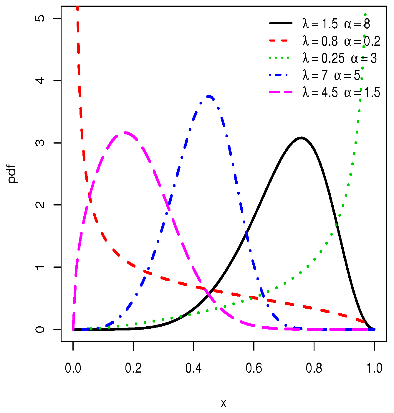
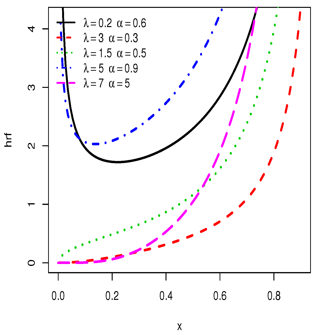
Some plots of the pdf and hrf of the TIHLTL distribution are displayed in Figure 1 and Figure 2, respectively. One can observe that the pdf can be left-skewed, right-skewed, approximate symmetrical, J-shaped, as well as reverse J-shaped, whereas the hrf can be increasing and bathtub shapes. This shows the great flexibility of the TIHLTL distribution and its potential in terms of data fitting.

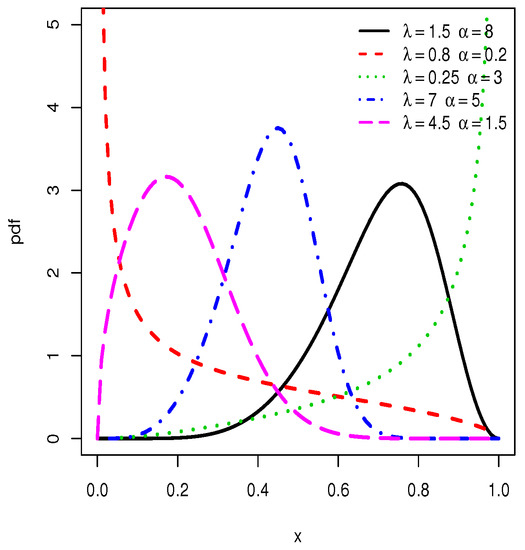
Figure 1. Plots for probability density functions (pdfs) of the type I half-logistic Topp–Leone (TIHLTL) distribution.

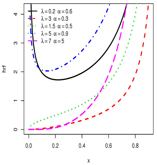
Figure 2. Plots for hazard rate functions (hrfs) of the type I half-logistic Topp–Leone (TIHLTL) distribution.

3. Mathematical Properties

In this section, some properties of the TIHLTL distribution are discussed.

3.1. Asymptotes and Shapes

Here, we investigate the influence of the parameters $\lambda$ and $\alpha$ on the asymptotes of the main functions of the TIHLTL distribution. When $x\to 0$, we have

$$F(x;\lambda ,\alpha )\sim \lambda 2^{\alpha -1}{x}^{\alpha },f(x;\lambda ,\alpha )\sim \lambda 2^{\alpha -1}\alpha x^{\alpha -1},h(x;\lambda ,\alpha )\sim \lambda 2^{\alpha -1}\alpha x^{\alpha -1}.$$

Thus, when $\alpha \in (0,1)$, we obtain $f(x;\lambda ,\alpha )\to +\infty$; when $\alpha =1$, we get $f(x;\lambda ,\alpha )\to \lambda$; and when $\alpha >1$, we have $f(x;\lambda ,\alpha )\to 0$. The same holds for $h(x;\lambda ,\alpha )$, under the same conditions.

When $x\to 1$, we have

$$1-F(x;\lambda ,\alpha )\sim 2{\alpha }^{\lambda }{(1-x)}^{2\lambda },f(x;\lambda ,\alpha )\sim 4\lambda {\alpha }^{\lambda }{(1-x)}^{2\lambda -1},h(x;\lambda ,\alpha )\sim 2\lambda {(1-x)}^{-1}.$$

Thus, when $\lambda \in (0,1/2)$, we have $f(x;\lambda ,\alpha )\to +\infty$; when $\lambda =1/2$, we obtain $f(x;\lambda ,\alpha )\to 2{\alpha }^{1/2}$; and when $\lambda >1/2$, we get $f(x;\lambda ,\alpha )\to 0$. We always have $h(x;\lambda ,\alpha )\to +\infty$.

The shapes of the pdf and hrf of the TIHLTL distribution can be described analytically. By adopting a common approach, the critical point(s) for $f(x;\lambda ,\alpha )$ is (are) the root(s) of the following equation: ${\left\{\log \left[f\right(x;\lambda ,\alpha \left)\right]\right\}}^{\prime }=0$, that is,

$$\begin{array}{c}\frac{2\alpha (x^2-2x+1)-x^2+2x-2}{x(1-x)(2-x)}-(\lambda -1)\frac{2\alpha x^{\alpha -1}(1-x){(2-x)}^{\alpha -1}}{1-x^{\alpha }{(2-x)}^{\alpha }}\hfill \\ +\frac{4\lambda \alpha x^{\alpha -1}(1-x){(2-x)}^{\alpha -1}{[1-x^{\alpha }{(2-x)}^{\alpha }]}^{\lambda -1}}{1+{[1-x^{\alpha }{(2-x)}^{\alpha }]}^{\lambda }}=0.\hfill \end{array}$$

The analytical expression for the solution(s) is clearly not available. However, for given $\alpha$ and $\lambda$, numerical evaluation of this(these) solution(s) is possible by the use of any mathematical software (e.g., Mathematica, R, etc.). As usual, if $x=x_{*}$ is a root of this equation, then the study of ${\upsilon }_{*}={\left\{\log \left[f\right(x;\lambda ,\alpha \left)\right]\right\}}^{″}{\mid }_{x=x_{*}}$ is useful to identify its nature; it is a local maximum if ${\upsilon }_{*}<0$, a local minimum if ${\upsilon }_{*}>0$, and it is a point of inflection if ${\upsilon }_{*}=0$.

Adopting a similar methodology, the critical point(s) for $h(x;\lambda ,\alpha )$ is(are) the root(s) of the following equation: ${\left\{\log \left[h\right(x;\lambda ,\alpha \left)\right]\right\}}^{\prime }=0$, that is,

$$\begin{array}{c}\frac{2\alpha (x^2-2x+1)-x^2+2x-2}{x(1-x)(2-x)}+\frac{2\alpha x^{\alpha -1}(1-x){(2-x)}^{\alpha -1}}{1-x^{\alpha }{(2-x)}^{\alpha }}\hfill \\ +\frac{2\lambda \alpha x^{\alpha -1}(1-x){(2-x)}^{\alpha -1}{[1-x^{\alpha }{(2-x)}^{\alpha }]}^{\lambda -1}}{1+{[1-x^{\alpha }{(2-x)}^{\alpha }]}^{\lambda }}=0.\hfill \end{array}$$

As usual, if $x=x_o$ is a root of this equation, then the study of ${\tau }_o={\left\{\log \left[h\right(x;\lambda ,\alpha \left)\right]\right\}}^{″}{\mid }_{x=x_o}$ is useful to identify its nature.

Hereafter, we consider a random variable (rv) X following the TIHLTL distribution, that is, having the cdf given by (1).

3.2. Quantile Function

The quantile function (qf) of X is given by the function $Q(y;\lambda ,\alpha )$ satisfying the equations: $F\left(Q\right(y;\lambda ,\alpha );\lambda ,\alpha )=Q\left(F\right(y;\lambda ,\alpha );\lambda ,\alpha )=y$, $y\in (0,1)$. After some algebraic manipulations, we obtain

$$Q(y;\lambda ,\alpha )=1-\sqrt{1-{\left(1-{\left[\frac{1-y}{1+y}\right]}^{1/\lambda }\right)}^{1/\alpha }},y\in (0,1).$$

In particular, the median of X is given by

$$M=Q\left(\frac{1}{2};\lambda ,\alpha \right)=1-\sqrt{1-{\left(1-{\left[\frac{1}{3}\right]}^{1/\lambda }\right)}^{1/\alpha }}.$$

Thanks to the qf, the TIHLTL distribution can be simulated as follows. For any rv U following the uniform distribution $\mathcal{U}(0,1)$, the rv $x_U=Q\left(U;\lambda ,\alpha \right)$ follows the TIHLTL distribution. Thus, with this formula, realization of U gives realizations of $x_U$. This aspect will be developed in Section 4.

Finally, upon differentiation of $Q(y;\lambda ,\alpha )$ with respect to y, the quantile density function given by

$$q(y;\lambda ,\alpha )=\frac{\left(\frac{1-y}{{(1+y)}^2}+\frac{1}{1+y}\right){\left(\frac{1-y}{1+y}\right)}^{1/\lambda -1}{\left[1-{\left(\frac{1-y}{1+y}\right)}^{1/\lambda }\right]}^{1/\alpha -1}}{2\lambda \alpha \sqrt{1-{\left(1-{\left[\frac{1-y}{1+y}\right]}^{1/\lambda }\right)}^{1/\alpha }}},y\in (0,1).$$

This function plays an important role in defining some useful statistical tools (see [18]).

3.3. Skewness and Kurtosis

The skewness and kurtosis of the TIHLTL distribution naturally depend on the values of $\lambda$ and $\alpha$. The precise effect of these parameters can be measured by the Bowley skewness and the Moors kurtosis, introduced by [19,20], respectively. They are both defined with the qf as, for the Bowley skewness,

$$S(\lambda ,\alpha )=\frac{Q(\frac{1}{4};\lambda ,\alpha )+Q(\frac{3}{4};\lambda ,\alpha )-2Q(\frac{1}{2};\lambda ,\alpha )}{Q(\frac{3}{4};\lambda ,\alpha )-Q(\frac{1}{4};\lambda ,\alpha )}$$

and, for the Moors kurtosis,

$$K(\lambda ,\alpha )=\frac{Q(\frac{7}{8};\lambda ,\alpha )-Q(\frac{5}{8};\lambda ,\alpha )+Q(\frac{3}{8};\lambda ,\alpha )-Q(\frac{1}{8};\lambda ,\alpha )}{Q(\frac{6}{8};\lambda ,\alpha )-Q(\frac{2}{8};\lambda ,\alpha )}.$$

The Bowley skewness and Moors kurtosis are well-known to be less sensitive to eventual outliers than other measures of skewness and kurtosis. As benchmark, for the standard normal distribution, we inform that the Bowley skewness is equal to 0 and the Moors kurtosis is equal to 1.233.

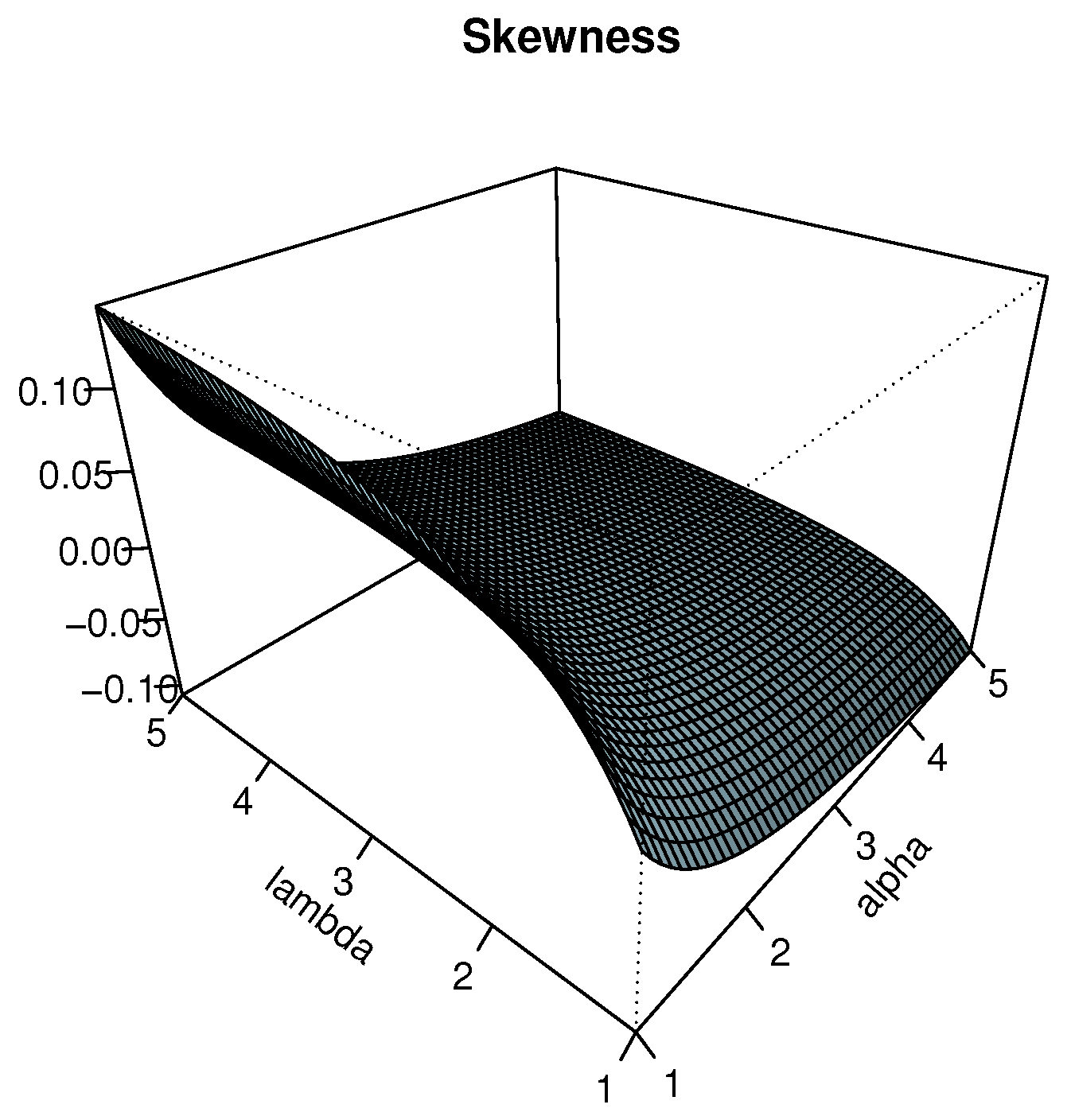
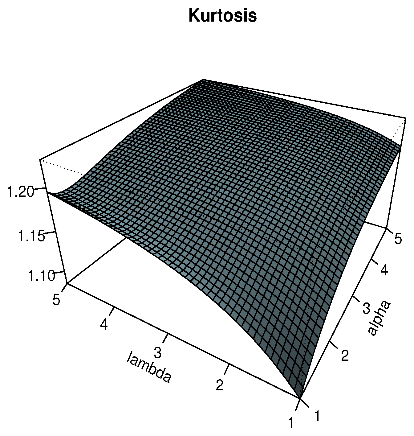
The plots of $S(\lambda ,\alpha )$ and $K(\lambda ,\alpha )$ are displayed in Figure 3 and Figure 4 for $\lambda ,\alpha \in (1,5)$, respectively. In particular, we see that the effects of $\alpha$ and $\lambda$ on $S(\lambda ,\alpha )$ are significant, showing negative and positive values, indicating negative and positive skewness properties, respectively. Also, we observe that the Moors kurtosis increases as $\lambda$ and $\alpha$ increase.

Figure 3. Plots for the Bowley skewness of the TIHLTL distribution.

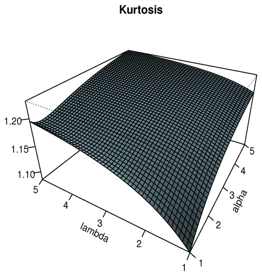
Figure 4. Plots for the Moors kurtosis of the TIHLTL distribution.

3.4. Power Series Expansion

The following result presents a useful power series expansion for $f(x;\lambda ,\alpha )$.

Proposition 1.

For any $x\in (0,1)$, we have the following power series expansion:

$$f(x;\lambda ,\alpha )=\sum _{k,\ell ,m=0}^{+\infty }{a}_{k,\ell ,m}{x}^{\alpha \ell +m-1},$$

where

$$a_{k,\ell ,m}=\left(\genfrac{}{}{0pt}{}{\lambda k}{\ell }\right)\left(\genfrac{}{}{0pt}{}{\alpha \ell }{m}\right){(-1)}^{k+\ell +m}{2}^{\alpha \ell -m+1}(\alpha \ell +m)$$

(with $a_{k,0,0}=0$, such that the sums can be considered without the conjoint value $(\ell ,m)=(0,0)$) and $\left(\genfrac{}{}{0pt}{}{v}{u}\right)$ denotes the generalized binomial coefficient defined by $\left(\genfrac{}{}{0pt}{}{v}{u}\right)=v(v-1)\dots (v-u+1)/u!$.

Proof. 

Since ${[1-x^{\alpha }{(2-x)}^{\alpha }]}^{\lambda }\in (0,1)$, by using the standard geometric formula, we have

$$\begin{array}{cc}\hfill F(x;\lambda ,\alpha )& =-1+2\frac{1}{1+{[1-x^{\alpha }{(2-x)}^{\alpha }]}^{\lambda }}=-1+2{\displaystyle \sum _{k=0}^{+\infty }}{(-1)}^k{[1-x^{\alpha }{(2-x)}^{\alpha }]}^{\lambda k}.\hfill \end{array}$$

Since $x^{\alpha }{(2-x)}^{\alpha }\in (0,1)$ and $x/2\in (0,1)$, by applying the generalized binomial formula two times in a row, we obtain

$$\begin{array}{c}\hfill {[1-x^{\alpha }{(2-x)}^{\alpha }]}^{\lambda k}={\displaystyle \sum _{\ell =0}^{+\infty }}\left(\genfrac{}{}{0pt}{}{\lambda k}{\ell }\right){(-1)}^{\ell }{x}^{\alpha \ell }{(2-x)}^{\alpha \ell }={\displaystyle \sum _{\ell ,m=0}^{+\infty }}\left(\genfrac{}{}{0pt}{}{\lambda k}{\ell }\right)\left(\genfrac{}{}{0pt}{}{\alpha \ell }{m}\right){(-1)}^{\ell +m}{2}^{\alpha \ell -m}{x}^{\alpha \ell +m}.\end{array}$$

By combining the above equalities, we get

$$\begin{array}{c}\hfill F(x;\lambda ,\alpha )=-1+{\displaystyle \sum _{k,\ell ,m=0}^{+\infty }}\left(\genfrac{}{}{0pt}{}{\lambda k}{\ell }\right)\left(\genfrac{}{}{0pt}{}{\alpha \ell }{m}\right){(-1)}^{k+\ell +m}{2}^{\alpha \ell -m+1}{x}^{\alpha \ell +m}.\end{array}$$

(4)

Upon differentiation, we obtain the desired result. This ends the proof of Proposition 1. □

The above result will be used to determine some structural properties of the TIHLTL distribution.

3.5. Ordinary Moments

In view of the asymptotes of $f(x;\lambda ,\alpha )$, for any positive integer r, the r-th ordinary moment of X exists. By using Proposition 1, we can express it as

$${\mu }_r^{\prime }=E\left(X^r\right)={\int }_0^1{x}^{r}f(x;\lambda ,\alpha )dx=\sum _{k,\ell ,m=0}^{+\infty }{a}_{k,\ell ,m}\frac{1}{r+\alpha \ell +m}.$$

Owing to this expression, the mean of X can be expressed as

$$\mu ={\mu }_1^{\prime }=\sum _{k,\ell ,m=0}^{+\infty }{a}_{k,\ell ,m}\frac{1}{1+\alpha \ell +m}.$$

Similarly, the variance of X is given by ${\sigma }^2={\mu }_2^{\prime }-{\mu }^2$. Other important quantities can be deduced, such as the r-th central moment of X given by

$$\begin{array}{c}\hfill {\mu }_r=E\left[{(X-\mu )}^r\right]={\displaystyle \sum _{k=0}^r}\left(\genfrac{}{}{0pt}{}{r}{k}\right){(-1)}^k{\mu }^k{\mu }_{r-k}^{\prime },\end{array}$$

as well as the skewness and kurtosis coefficients of X based on central moments given by, respectively,

$$\begin{array}{c}\hfill S\left(X\right)=\frac{{\mu }_3}{{\mu }_2^{3/2}},K\left(X\right)=\frac{{\mu }_4}{{\mu }_2^2}.\end{array}$$

As the Bowley skewness and Moors kurtosis, these two coefficients are of importance because they measure the asymmetry and the peakedness of the TIHLTL distribution, respectively.

3.6. Incomplete Moments

Let A be an event and $1_A$ be the rv such that $1_A=1$ if the event A is realized, and 0 otherwise. Then, for any $t\in (0,1)$, the r-th incomplete moment of X is given by

$${\mu }_r^{\prime }\left(t\right)=E\left(X^r{1}_{\{X\le t\}}\right)={\int }_0^t{x}^{r}f(x;\lambda ,\alpha )dx=\sum _{k,\ell ,m=0}^{+\infty }{a}_{k,\ell ,m}\frac{t^{r+\alpha \ell +m}}{r+\alpha \ell +m}.$$

In particular, the incomplete mean of X is given by

$${\mu }_1^{\prime }\left(t\right)=\sum _{k,\ell ,m=0}^{+\infty }{a}_{k,\ell ,m}\frac{t^{1+\alpha \ell +m}}{1+\alpha \ell +m}.$$

Other important probabilistic quantities include the mean and the mean of X about the median, respectively given by

$$\begin{array}{c}\hfill {\delta }_1=E\left(\right|X-\mu \left|\right)=2\mu F(\mu ;\lambda ,\alpha )-2{\mu }_1^{\prime }\left(\mu \right),{\delta }_2=E\left(\right|X-M\left|\right)=\mu -2{\mu }_1^{\prime }\left(M\right).\end{array}$$

3.7. Moment-Generating Function

The moment-generating function of X is obtained as, for $t\in \mathbb{R}$,

$$\begin{array}{c}\hfill M\left(t\right)=E\left(e^{tX}\right)={\int }_0^1{e}^{tx}f(x;\lambda ,\alpha )dx={\displaystyle \sum _{k,\ell ,m=0}^{+\infty }}{a}_{k,\ell ,m}{\int }_0^1{x}^{\alpha \ell +m-1}{e}^{tx}dx.\end{array}$$

The last integral term can be calculated in different manners according to the value of t. For instance, if $t\le 0$, one can remark that ${\int }_0^1{x}^{\alpha \ell +m-1}{e}^{tx}dx={(-t)}^{-\alpha \ell -m}\gamma (\alpha \ell +m,-t)$, where $\gamma (s,x)$ denotes the lower incomplete gamma function defined by $\gamma (s,x)={\int }_0^x{u}^{s-1}{e}^{-u}du$. Another point of view is to consider the power series of the exponential function: for any $t\in \mathbb{R}$, we have

$$\begin{array}{c}\hfill {\int }_0^1{x}^{\alpha \ell +m-1}{e}^{tx}dx={\displaystyle \sum _{k=0}^{+\infty }}\frac{t^k}{k!(k+\alpha m+\ell )}.\end{array}$$

3.8. Stress Strength Parameter

Here, we derive the stress strength parameter defined by $R=P(X_2<X_1)$, when $X_1$ and $X_2$ are independent rvs following the TIHLTL distribution with the parameters $({\lambda }_1,{\alpha }_1)$ and $({\lambda }_2,{\alpha }_2)$, respectively. The parameter R is central in reliability theory and deserves special treatment in our context. Further details can be found in [21]. First of all, let ${\mu }_0^{\prime \left(1\right)}=1$ and, for any $r>0$,

$${\mu }_r^{\prime \left(1\right)}=E\left(X_1^r\right)=\sum _{u,v,w=0}^{+\infty }{a}_{u,v,w}^{\left(1\right)}\frac{1}{r+{\alpha }_{1}v+w},$$

where $a_{u,v,w}^{\left(1\right)}=\left(\genfrac{}{}{0pt}{}{{\lambda }_{1}u}{v}\right)\left(\genfrac{}{}{0pt}{}{{\alpha }_{1}v}{w}\right){(-1)}^{u+v+w}{2}^{{\alpha }_{1}v-w+1}({\alpha }_{1}v+w)$. Then, by virtue of the expression of $F(x;{\lambda }_2,{\alpha }_2)$ given by (4), we have

$$\begin{array}{cc}\hfill R& ={\int }_0^{1}F(x;{\lambda }_2,{\alpha }_2)f(x;{\lambda }_1,{\alpha }_1)dx=-1+{\displaystyle \sum _{k,\ell ,m=0}^{+\infty }}\left(\genfrac{}{}{0pt}{}{{\lambda }_{2}k}{\ell }\right)\left(\genfrac{}{}{0pt}{}{{\alpha }_2\ell }{m}\right){(-1)}^{k+\ell +m}{2}^{{\alpha }_2\ell -m+1}{\mu }_{{\alpha }_2\ell +m}^{\prime \left(1\right)}.\hfill \end{array}$$

When ${\lambda }_1={\lambda }_2$ and ${\alpha }_1={\alpha }_2$, we have $R=1/2$.

3.9. Order Statistics

Many natural phenomena can be modeled by the so-called order statistics, explaining their importance for statisticians. The complete theory can be found in [22]. Here, we provide a contribution to the subject by investigating some properties of the order statistics for the TIHLTL distribution. Let $X_1,\dots ,X_n$ be n independent and identically distributed rvs following the TIHLTL distribution. Then, the i-th order statistic is defined by the i-th rv $X_{\left(i\right)}$ such that, after reordering of $X_1,\dots ,X_n$ in an ascending manner, $X_{\left(1\right)}\le X_{\left(2\right)}\le \dots \le X_{\left(n\right)}$. Then, a well-established result states that the pdf of the i-th order statistic is given by

$$\begin{array}{c}\hfill f_{\left(i\right)}(x;\lambda ,\alpha )=c_{i,n}f(x;\lambda ,\alpha )F{(x;\lambda ,\alpha )}^{i-1}{\left[1-F(x;\lambda ,\alpha )\right]}^{n-i},x\in (0,1),\end{array}$$

where $c_{i,n}=n!/[(i-1)!(n-i)!]$. As an alternative expression, the binomial formula gives

$$\begin{array}{c}\hfill f_{\left(i\right)}(x;\lambda ,\alpha )=c_{i,n}{\displaystyle \sum _{j=0}^{n-i}}\left(\genfrac{}{}{0pt}{}{n-i}{j}\right){(-1)}^{j}f(x;\lambda ,\alpha )F{(x;\lambda ,\alpha )}^{j+i-1}.\end{array}$$

The following result provides a series expansion for the exponentiated cdf $F(x;\lambda ,\alpha )$.

Proposition 2.

Let τ be a positive integer. Then, we have the following power series expansion:

$$\begin{array}{c}\hfill F{(x;\lambda ,\alpha )}^{\tau }={\displaystyle \sum _{u=0}^{\tau }}{\displaystyle \sum _{v,w,z=0}^{+\infty }}{b}_{u,v,w,z}^{\left(\tau \right)}{x}^{\alpha w+z},\end{array}$$

where

$$\begin{array}{c}\hfill b_{u,v,w,z}^{\left(\tau \right)}=\left(\genfrac{}{}{0pt}{}{\tau }{u}\right)\left(\genfrac{}{}{0pt}{}{-u}{v}\right)\left(\genfrac{}{}{0pt}{}{\lambda v}{w}\right)\left(\genfrac{}{}{0pt}{}{\alpha w}{z}\right){(-1)}^{w+z+\tau -u}{2}^{u+\alpha w-z}.\end{array}$$

Proof. 

We adopt a different strategy to the proof of Proposition 1. Since ${[1-x^{\alpha }{(2-x)}^{\alpha }]}^{\lambda }\in (0,1)$, it follows from the (standard and generalized) binomial formula that

$$\begin{array}{cc}\hfill F{(x;\lambda ,\alpha )}^{\tau }& ={\left\{-1+2\frac{1}{1+{[1-x^{\alpha }{(2-x)}^{\alpha }]}^{\lambda }}\right\}}^{\tau }={\displaystyle \sum _{u=0}^{\tau }}\left(\genfrac{}{}{0pt}{}{\tau }{u}\right){(-1)}^{\tau -u}{2}^u{\left\{1+{[1-x^{\alpha }{(2-x)}^{\alpha }]}^{\lambda }\right\}}^{-u}\hfill \\ & ={\displaystyle \sum _{u=0}^{\tau }}{\displaystyle \sum _{v=0}^{+\infty }}\left(\genfrac{}{}{0pt}{}{\tau }{u}\right)\left(\genfrac{}{}{0pt}{}{-u}{v}\right){(-1)}^{\tau -u}{2}^u{[1-x^{\alpha }{(2-x)}^{\alpha }]}^{\lambda v}.\hfill \end{array}$$

Since $x^{\alpha }{(2-x)}^{\alpha }\in (0,1)$ and $x/2\in (0,1)$, by applying the binomial formula two times in a row, we obtain

$$\begin{array}{c}\hfill {[1-x^{\alpha }{(2-x)}^{\alpha }]}^{\lambda v}={\displaystyle \sum _{w=0}^{+\infty }}\left(\genfrac{}{}{0pt}{}{\lambda v}{w}\right){(-1)}^w{x}^{\alpha w}{(2-x)}^{\alpha w}={\displaystyle \sum _{w,z=0}^{+\infty }}\left(\genfrac{}{}{0pt}{}{\lambda v}{w}\right)\left(\genfrac{}{}{0pt}{}{\alpha w}{z}\right){(-1)}^{w+z}{2}^{\alpha w-z}{x}^{\alpha w+z}.\end{array}$$

By combining the above equalities, we obtain the desired result. This ends the proof of Proposition 2. □

By Proposition 2, upon differentiation of $F{(x;\lambda ,\alpha )}^{j+i}$, we obtain the following series expansion:

$$\begin{array}{c}\hfill f(x;\lambda ,\alpha )F{(x;\lambda ,\alpha )}^{j+i-1}=\frac{1}{j+i}{\displaystyle \sum _{u=0}^{j+i}}{\displaystyle \sum _{v,w,z=0}^{+\infty }}{b}_{u,v,w,z}^{(j+i)}(\alpha w+z)x^{\alpha w+z-1}.\end{array}$$

Therefore, we can write

$$\begin{array}{c}\hfill f_{\left(i\right)}(x;\lambda ,\alpha )={\displaystyle \sum _{j=0}^{n-i}}{\displaystyle \sum _{u=0}^{j+i}}{\displaystyle \sum _{v,w,z=0}^{+\infty }}{d}_{i,j,n,u,v,w,z}{x}^{\alpha w+z-1},\end{array}$$

where

$$\begin{array}{c}\hfill d_{i,j,n,u,v,w,z}=c_{i,n}\left(\genfrac{}{}{0pt}{}{n-i}{j}\right)\frac{1}{j+i}{(-1)}^j{b}_{u,v,w,z}^{(j+i)}(\alpha w+z).\end{array}$$

From this expression, one can derive several interesting structural properties on the i-th order statistic, such as the r-th ordinary moment, that is,

$${\mu }_{\left(i\right),r}^{\prime }=E\left(X_{\left(i\right)}^r\right)=\sum _{j=0}^{n-i}\sum _{u=0}^{j+i}\sum _{v,w,z=0}^{+\infty }{d}_{i,j,n,u,v,w,z}\frac{1}{r+\alpha w+z}.$$

4. Parameter Estimation

We now explore the statistical aspect of the TIHLTL distribution and investigate the estimation of the unknown parameters $\lambda$ and $\alpha$ by seven methods. Hereafter, $x_1,\dots ,x_n$ denote realizations from a random sample of size n from X, and $x_{\left(1\right)},\dots ,x_{\left(n\right)}$ their values in ascending order.

4.1. Method of Maximum Likelihood Estimation

The most useful parametric estimation method is the maximum likelihood method. The reason for its popularity is explained by the theoretical guarantees of the resulting estimators; they enjoy tractable properties such as consistency and asymptotic normality, allowing the construction of reliable objects as confidence interval or statistical tests. See, for instance, [23]. The essential of the method of maximum likelihood estimation in the context of the TIHLTL model is described below. Here, the maximum likelihood estimates (MLEs) of $\lambda$ and $\alpha$ can be obtained by maximizing, with respect to $\lambda$ and $\alpha$, the log-likelihood function for $(\lambda ,\alpha )$ given by

$$\begin{array}{cc}\hfill \ell (\lambda ,\alpha )& ={\displaystyle \sum _{i=1}^n}\log \left[f(x_i;\lambda ,\alpha )\right]\hfill \\ & =n\log \left(4\right)+n\log \left(\lambda \right)+n\log \left(\alpha \right)+(\alpha -1){\displaystyle \sum _{i=1}^n}\log \left(x_i\right)+{\displaystyle \sum _{i=1}^n}\log (1-x_i)\hfill \\ & +(\alpha -1){\displaystyle \sum _{i=1}^n}\log (2-x_i)+(\lambda -1){\displaystyle \sum _{i=1}^n}\log [1-x_i^{\alpha }{(2-x_i)}^{\alpha }]-2{\displaystyle \sum _{i=1}^n}\log \left\{1+{[1-x_i^{\alpha }{(2-x_i)}^{\alpha }]}^{\lambda }\right\}.\hfill \end{array}$$

Thus, the maximum likelihood estimates can be determined by solving the following equations simultaneously: $\partial \ell (\lambda ,\alpha )/\partial \lambda =0$ and $\partial \ell (\lambda ,\alpha )/\partial \alpha =0$, where

$$\begin{array}{c}\hfill \frac{\partial \ell (\lambda ,\alpha )}{\partial \lambda }=\frac{n}{\lambda }+{\displaystyle \sum _{i=1}^n}\log [1-x_i^{\alpha }{(2-x_i)}^{\alpha }]-2{\displaystyle \sum _{i=1}^n}\frac{{[1-x_i^{\alpha }{(2-x_i)}^{\alpha }]}^{\lambda }\log [1-x_i^{\alpha }{(2-x_i)}^{\alpha }]}{1+{[1-x_i^{\alpha }{(2-x_i)}^{\alpha }]}^{\lambda }}\end{array}$$

and

$$\begin{array}{c}\frac{\partial \ell (\lambda ,\alpha )}{\partial \alpha }=\frac{n}{\alpha }+{\displaystyle \sum _{i=1}^n}\log \left(x_i\right)+{\displaystyle \sum _{i=1}^n}\log (2-x_i)-(\lambda -1){\displaystyle \sum _{i=1}^n}\frac{x_i^{\alpha }{(2-x_i)}^{\alpha }\log \left[x_i(2-x_i)\right]}{1-x_i^{\alpha }{(2-x_i)}^{\alpha }}\hfill \\ +2\lambda {\displaystyle \sum _{i=1}^n}\frac{x_i^{\alpha }{(2-x_i)}^{\alpha }\log \left[x_i(2-x_i)\right]{[1-x_i^{\alpha }{(2-x_i)}^{\alpha }]}^{\lambda -1}}{1+{[1-x_i^{\alpha }{(2-x_i)}^{\alpha }]}^{\lambda }}.\hfill \end{array}$$

Owing to the complexity of these equations, the MLEs do not have analytical expression. However, one can use standard statistical software to solve them (e.g., Mathematica, R, etc.). In this study, R was be used.

4.2. Methods of Least Squares and Weighted Least Squares Estimation

We now consider the methods of least squares and weighted least squares estimation introduced by [24]. The least square estimates (LSEs) of $\lambda$ and $\alpha$ can be determined by minimizing, with respect to $\lambda$ and $\alpha$, the least square function defined by

$$LS(\lambda ,\alpha )=\sum _{i=1}^n{\left[F(x_{\left(i\right)};\lambda ,\alpha )-\frac{i}{n+1}\right]}^2=\sum _{i=1}^n{\left[\frac{1-{[1-x_{\left(i\right)}^{\alpha }{(2-x_{\left(i\right)})}^{\alpha }]}^{\lambda }}{1+{[1-x_{\left(i\right)}^{\alpha }{(2-x_{\left(i\right)})}^{\alpha }]}^{\lambda }}-\frac{i}{n+1}\right]}^2.$$

Thus, the least square estimates can be obtained by solving the following equations simultaneously: $\partial LS(\lambda ,\alpha )/\partial \lambda =0$ and $\partial LS(\lambda ,\alpha )/\partial \alpha =0$, where

$$\begin{array}{c}\hfill \frac{\partial LS(\lambda ,\alpha )}{\partial \lambda }=2{\displaystyle \sum _{i=1}^n}{\eta }_i^{\left(1\right)}(\lambda ,\alpha )\left[\frac{1-{[1-x_{\left(i\right)}^{\alpha }{(2-x_{\left(i\right)})}^{\alpha }]}^{\lambda }}{1+{[1-x_{\left(i\right)}^{\alpha }{(2-x_{\left(i\right)})}^{\alpha }]}^{\lambda }}-\frac{i}{n+1}\right]\end{array}$$

and

$$\begin{array}{c}\hfill \frac{\partial LS(\lambda ,\alpha )}{\partial \alpha }=2{\displaystyle \sum _{i=1}^n}{\eta }_i^{\left(2\right)}(\lambda ,\alpha )\left[\frac{1-{[1-x_{\left(i\right)}^{\alpha }{(2-x_{\left(i\right)})}^{\alpha }]}^{\lambda }}{1+{[1-x_{\left(i\right)}^{\alpha }{(2-x_{\left(i\right)})}^{\alpha }]}^{\lambda }}-\frac{i}{n+1}\right],\end{array}$$

where

$$\begin{array}{c}\hfill {\eta }_i^{\left(1\right)}(\lambda ,\alpha )=-2\frac{{[1-x_{\left(i\right)}^{\alpha }{(2-x_{\left(i\right)})}^{\alpha }]}^{\lambda }\log [1-x_{\left(i\right)}^{\alpha }{(2-x_{\left(i\right)})}^{\alpha }]}{{\left\{1+{[1-x_{\left(i\right)}^{\alpha }{(2-x_{\left(i\right)})}^{\alpha }]}^{\lambda }\right\}}^2}\end{array}$$

(5)

and

$$\begin{array}{c}\hfill {\eta }_i^{\left(2\right)}(\lambda ,\alpha )=2\lambda \frac{x_{\left(i\right)}^{\alpha }{(2-x_{\left(i\right)})}^{\alpha }\log \left[x_{\left(i\right)}(2-x_{\left(i\right)})\right]{[1-x_{\left(i\right)}^{\alpha }{(2-x_{\left(i\right)})}^{\alpha }]}^{\lambda -1}}{{\left\{1+{[1-x_{\left(i\right)}^{\alpha }{(2-x_{\left(i\right)})}^{\alpha }]}^{\lambda }\right\}}^2}.\end{array}$$

(6)

The weighted least square estimates (WLSEs) of $\lambda$ and $\alpha$ can be obtained by minimizing, with respect to $\lambda$ and $\alpha$, the weighted least square function defined by

$$\begin{array}{cc}\hfill LSW(\lambda ,\alpha )& ={\displaystyle \sum _{i=1}^n}\frac{{(n+1)}^2(n+2)}{i(n-i+1)}{\left[F(x_{\left(i\right)};\lambda ,\alpha )-\frac{i}{n+1}\right]}^2\hfill \\ & ={\displaystyle \sum _{i=1}^n}\frac{{(n+1)}^2(n+2)}{i(n-i+1)}{\left[\frac{1-{[1-x_{\left(i\right)}^{\alpha }{(2-x_{\left(i\right)})}^{\alpha }]}^{\lambda }}{1+{[1-x_{\left(i\right)}^{\alpha }{(2-x_{\left(i\right)})}^{\alpha }]}^{\lambda }}-\frac{i}{n+1}\right]}^2.\hfill \end{array}$$

Then, one can set similar equations developed for $LS(\lambda ,\alpha )$.

4.3. Method of Cramer–von Mises Minimum Distance Estimation

The Cramer–von Mises minimum distance estimates (CVEs) of $\lambda$ and $\alpha$ can be determined by minimizing, with respect to $\lambda$ and $\alpha$, the Cramer–von Mises minimum distance function defined by

$$\begin{array}{c}\hfill C(\lambda ,\alpha )=\frac{1}{12n}+{\displaystyle \sum _{i=1}^n}{\left[F(x_{\left(i\right)};\lambda ,\alpha )-\frac{2i-1}{2n}\right]}^2=\frac{1}{12n}+{\displaystyle \sum _{i=1}^n}{\left[\frac{1-{[1-x_{\left(i\right)}^{\alpha }{(2-x_{\left(i\right)})}^{\alpha }]}^{\lambda }}{1+{[1-x_{\left(i\right)}^{\alpha }{(2-x_{\left(i\right)})}^{\alpha }]}^{\lambda }}-\frac{2i-1}{2n}\right]}^2.\end{array}$$

Thus, the Cramer–von Mises minimum distance estimates can be obtained by solving the following equations simultaneously: $\partial C(\lambda ,\alpha )/\partial \lambda =0$ and $\partial C(\lambda ,\alpha )/\partial \alpha =0$, where

$$\begin{array}{c}\hfill \frac{\partial C(\lambda ,\alpha )}{\partial \lambda }=2{\displaystyle \sum _{i=1}^n}{\eta }_i^{\left(1\right)}(\lambda ,\alpha )\left[\frac{1-{[1-x_{\left(i\right)}^{\alpha }{(2-x_{\left(i\right)})}^{\alpha }]}^{\lambda }}{1+{[1-x_{\left(i\right)}^{\alpha }{(2-x_{\left(i\right)})}^{\alpha }]}^{\lambda }}-\frac{2i-1}{2n}\right]\end{array}$$

and

$$\begin{array}{c}\hfill \frac{\partial C(\lambda ,\alpha )}{\partial \alpha }=2{\displaystyle \sum _{i=1}^n}{\eta }_i^{\left(2\right)}(\lambda ,\alpha )\left[\frac{1-{[1-x_{\left(i\right)}^{\alpha }{(2-x_{\left(i\right)})}^{\alpha }]}^{\lambda }}{1+{[1-x_{\left(i\right)}^{\alpha }{(2-x_{\left(i\right)})}^{\alpha }]}^{\lambda }}-\frac{2i-1}{2n}\right],\end{array}$$

${\eta }_i^{\left(1\right)}(\lambda ,\alpha )$ and ${\eta }_i^{\left(2\right)}(\lambda ,\alpha )$ are given by (5) and (6), respectively. Further detail on this method can be found in [25].

4.4. Method of Percentile Estimation

The method of percentile estimation was introduced by [26,27] in the context of the Weibull distribution, and has been generalized to other distributions. Here, the percentile estimates (PCEs) of $\lambda$ and $\alpha$ can be obtained by minimizing, with respect to $\lambda$ and $\alpha$, the function defined by

$$\begin{array}{c}\hfill U(\lambda ,\alpha )={\displaystyle \sum _{i=1}^n}{\left[x_{\left(i\right)}-Q(p_i;\lambda ,\alpha )\right]}^2={\displaystyle \sum _{i=1}^n}{\left[x_{\left(i\right)}-1+\sqrt{1-{\left(1-{\left[\frac{1-p_i}{1+p_i}\right]}^{1/\lambda }\right)}^{1/\alpha }}\right]}^2,\end{array}$$

where $p_i=(i+1)/n$. Thus, the percentile estimates can be determined by solving the following equations simultaneously: $\partial U(\lambda ,\alpha )/\partial \lambda =0$ and $\partial U(\lambda ,\alpha )/\partial \alpha =0$, where

$$\begin{array}{c}\hfill \frac{\partial U(\lambda ,\alpha )}{\partial \lambda }=2{\displaystyle \sum _{i=1}^n}{\upsilon }_i^{\left(1\right)}(\lambda ,\alpha )\left[x_{\left(i\right)}-1+\sqrt{1-{\left(1-{\left[\frac{1-p_i}{1+p_i}\right]}^{1/\lambda }\right)}^{1/\alpha }}\right]\end{array}$$

and

$$\begin{array}{c}\hfill \frac{\partial U(\lambda ,\alpha )}{\partial \alpha }=2{\displaystyle \sum _{i=1}^n}{\upsilon }_i^{\left(2\right)}(\lambda ,\alpha )\left[x_{\left(i\right)}-1+\sqrt{1-{\left(1-{\left[\frac{1-p_i}{1+p_i}\right]}^{1/\lambda }\right)}^{1/\alpha }}\right],\end{array}$$

where

$$\begin{array}{c}\hfill {\upsilon }_i^{\left(1\right)}(\lambda ,\alpha )=-\frac{{\left[\frac{1-p_i}{1+p_i}\right]}^{1/\lambda }\log \left(\frac{1-p_i}{1+p_i}\right){\left(1-{\left[\frac{1-p_i}{1+p_i}\right]}^{1/\lambda }\right)}^{1/\alpha -1}}{2\alpha {\lambda }^2\sqrt{1-{\left(1-{\left[\frac{1-p_i}{1+p_i}\right]}^{1/\lambda }\right)}^{1/\alpha }}}\end{array}$$

and

$$\begin{array}{c}\hfill {\upsilon }_i^{\left(2\right)}(\lambda ,\alpha )=\frac{{\left(1-{\left[\frac{1-p_i}{1+p_i}\right]}^{1/\lambda }\right)}^{1/\alpha }\log \left(1-{\left[\frac{1-p_i}{1+p_i}\right]}^{1/\lambda }\right)}{2{\alpha }^2\sqrt{1-{\left(1-{\left[\frac{1-p_i}{1+p_i}\right]}^{1/\lambda }\right)}^{1/\alpha }}}.\end{array}$$

4.5. Methods of Anderson–Darling and Right-Tail Anderson–Darling Estimation

The method of Anderson–Darling estimation was introduced by [28] in the context of statistical tests. By adapting it to the TIHLTL model, the Anderson–Darling estimates (ADEs) of $\lambda$ and $\alpha$ can be determined by minimizing, with respect to $\lambda$ and $\alpha$, the function given by

$$\begin{array}{c}\hfill A(\lambda ,\alpha )=-n-\frac{1}{n}{\displaystyle \sum _{i=1}^n}(2i-1)\left\{\log \left[F(x_{\left(i\right)};\lambda ,\alpha )\right]+\log [1-F(x_{(n+1-i)};\lambda ,\alpha )]\right\}.\end{array}$$

Thus, the Anderson–Darling estimates can be obtained by solving the following equations simultaneously: $\partial A(\lambda ,\alpha )/\partial \lambda =0$ and $\partial A(\lambda ,\alpha )/\partial \alpha =0$, where

$$\begin{array}{c}\hfill \frac{\partial A(\lambda ,\alpha )}{\partial \lambda }=-\frac{1}{n}{\displaystyle \sum _{i=1}^n}(2i-1)\left[\frac{{\eta }_i^{\left(1\right)}(\lambda ,\alpha )}{F(x_{\left(i\right)};\lambda ,\alpha )}-\frac{{\eta }_{n+1-i}^{\left(1\right)}(\lambda ,\alpha )}{1-F(x_{(n+1-i)};\lambda ,\alpha )}\right]\end{array}$$

and

$$\begin{array}{c}\hfill \frac{\partial A(\lambda ,\alpha )}{\partial \alpha }=-\frac{1}{n}{\displaystyle \sum _{i=1}^n}(2i-1)\left[\frac{{\eta }_i^{\left(2\right)}(\lambda ,\alpha )}{F(x_{\left(i\right)};\lambda ,\alpha )}-\frac{{\eta }_{n+1-i}^{\left(2\right)}(\lambda ,\alpha )}{1-F(x_{(n+1-i)};\lambda ,\alpha )}\right],\end{array}$$

${\eta }_i^{\left(1\right)}(\lambda ,\alpha )$ and ${\eta }_i^{\left(2\right)}(\lambda ,\alpha )$ are given by (5) and (6), respectively. Similarly, the right-tail Anderson–Darling estimates (RTADEs) of $\lambda$ and $\alpha$ can be determined by minimizing, with respect to $\lambda$ and $\alpha$, the function given by

$$\begin{array}{c}\hfill R(\lambda ,\alpha )=\frac{n}{2}-2{\displaystyle \sum _{i=1}^n}\log \left[F(x_{\left(i\right)};\lambda ,\alpha )\right]-\frac{1}{n}{\displaystyle \sum _{i=1}^n}(2i-1)\log [1-F(x_{(n+1-i)};\lambda ,\alpha )].\end{array}$$

Thus, the right-tail Anderson–Darling estimates can be obtained by solving the following equations simultaneously: $\partial R(\lambda ,\alpha )/\partial \lambda =0$ and $\partial R(\lambda ,\alpha )/\partial \alpha =0$, where

$$\begin{array}{c}\hfill \frac{\partial R(\lambda ,\alpha )}{\partial \lambda }=-2{\displaystyle \sum _{i=1}^n}\frac{{\eta }_i^{\left(1\right)}(\lambda ,\alpha )}{F(x_{\left(i\right)};\lambda ,\alpha )}+\frac{1}{n}{\displaystyle \sum _{i=1}^n}(2i-1)\frac{{\eta }_{n+1-i}^{\left(1\right)}(\lambda ,\alpha )}{1-F(x_{(n+1-i)};\lambda ,\alpha )}\end{array}$$

and

$$\begin{array}{c}\hfill \frac{\partial R(\lambda ,\alpha )}{\partial \alpha }=-2{\displaystyle \sum _{i=1}^n}\frac{{\eta }_i^{\left(2\right)}(\lambda ,\alpha )}{F(x_{\left(i\right)};\lambda ,\alpha )}+\frac{1}{n}{\displaystyle \sum _{i=1}^n}(2i-1)\frac{{\eta }_{n+1-i}^{\left(2\right)}(\lambda ,\alpha )}{1-F(x_{(n+1-i)};\lambda ,\alpha )}.\end{array}$$

4.6. Simulation

Here, we came up with a numerical study to compare the behavior of the previously introduced estimates. We generated N = 1000 random samples of size n = 50, 100, 200 and 1000 from the TIHLTL distribution. Six sets of the parameters were assigned as $i:(\alpha =2,\lambda =0.5)$, $ii:(\alpha =2,\lambda =1.5)$, $iii:(\alpha =2,\lambda =2)$, $iv:(\alpha =3,\lambda =0.5)$, $v:(\alpha =3,\lambda =1.5)$, and $vi:(\alpha =3,\lambda =2)$. The MLE, LSE, WLSE, PCE, CVE, ADE, and RTADE of $\alpha$ and $\lambda$ were determined for each sample, allowing the calculus of the mean estimates (Est.) for these methods. We also evaluated the mean square errors (MSEs) defined by

$$MSE=\frac{1}{N}\sum _{i=1}^N{({\widehat{ϵ}}_i-ϵ)}^2,$$

where $ϵ$ is $\alpha$ or $\lambda$, and ${\widehat{ϵ}}_i$ denotes the corresponding estimates constructed with the i-th random sample. The obtained values are collected in Table 1, Table 2, Table 3, Table 4, Table 5 and Table 6: Table 1 for i, Table 2 for $ii$, Table 3 for $iii$, Table 4 for $iv$, Table 5 for v, and Table 6 for $vi$.

Table 1. Simulations with the seven methods of estimation for $\alpha =2$ and $\lambda =0.5$.

	MLE		LSE		WLSE		PCE		CVE		ADE		RTADE
n	Est.	MSEs	Est.	MSEs	Est.	MSEs	Est.	MSEs	Est.	MSEs	Est.	MSEs	Est.	MSEs
50	2.172	0.628	2.038	0.473	2.058	0.508	1.808	0.583	2.148	3.377	2.067	2.974	2.194	3.811
	0.507	7.116 *	0.499	5.885 *	0.498	6.713 *	0.472	0.013	0.499	6.241 *	0.499	6.682 *	0.498	7.554 *
100	2.164	0.271	2.011	0.206	2.062	0.340	1.852	0.272	2.159	3.139	2.064	2.766	2.131	3.288
	0.515	2.525 *	0.499	2.756 *	0.495	2.766 *	0.473	7.531 *	0.515	3.873 *	0.496	2.697 *	0.501	3.809 *
200	2.106	0.098	2.023	0.157	2.029	0.107	1.912	0.130	2.057	2.587	2.015	2.379	2.030	2.532
	0.503	1.184 *	0.500	1.891 *	0.502	1.514 *	0.488	4.459 *	0.501	1.827 *	0.501	1.220 *	0.501	1.848 *
1000	1.997	0.057	2.012	0.024	2.012	0.019	1.998	0.039	2.020	2.334	2.010	2.298	2.027	2.365
	0.499	1.381 *	0.501	0.313 *	0.501	0.247 *	0.503	1.741 *	0.502	0.317 *	0.501	0.251 *	0.502	0.324 *

* Indicates that the value is multiplied by ${10}^{-3}$. ADE: Anderson–Darling estimate; CVE: Cramer–von Mises minimum distance estimate; Est.: mean estimate; LSE: least square estimate; MLE: maximum likelihood estimate; MSE: mean square error; PCE: percentile estimate; RTADE: right-tail ADE; WLSE: weighted LSE.

Table 2. Simulations with the seven methods of estimation for $\alpha =2$ and $\lambda =1.5$.

	MLE		LSE		WLSE		PCE		CVE		ADE		RTADE
n	Est.	MSEs	Est.	MSEs	Est.	MSEs	Est.	MSEs	Est.	MSEs	Est.	MSEs	Est.	MSEs
50	2.136	0.213	1.949	0.188	2.049	0.210	1.794	0.272	2.092	0.614	2.043	0.456	2.130	0.679
	1.593	0.106	1.465	0.064	1.538	0.114	1.350	0.153	1.588	0.135	1.552	0.081	1.573	0.136
100	2.063	0.077	2.051	0.130	2.008	0.118	1.780	0.181	2.079	0.438	2.012	0.346	2.069	0.470
	1.535	0.033	1.539	0.051	1.502	0.046	1.333	0.167	1.565	0.050	1.504	0.030	1.535	0.050
200	2.026	0.047	2.016	0.057	2.021	0.047	1.850	0.085	2.055	0.370	2.011	0.312	2.042	0.340
	1.529	0.018	1.516	0.026	1.528	0.022	1.387	0.069	1.543	0.030	1.503	0.022	1.540	0.021
1000	2.009	7.847 *	2.007	0.010	2.008	8.377 *	1.961	0.016	2.012	0.272	2.006	0.265	2.014	0.276
	1.507	3.286 *	1.505	4.59 *1	1.506	3.595 *	1.465	0.013	1.509	4.675 *	1.505	3.699 *	1.510	4.574 *

* Indicates that the value is multiplied by ${10}^{-3}$.

Table 3. Simulations with the seven methods of estimation for $\alpha =2$ and $\lambda =2$.

	MLE		LSE		WLSE		PCE		CVE		ADE		RTADE
n	Est.	MSEs	Est.	MSEs	Est.	MSEs	Est.	MSEs	Est.	MSEs	Est.	MSEs	Est.	MSEs
50	2.065	0.164	2.034	0.199	2.060	0.204	1.781	0.274	2.104	0.238	2.012	0.157	2.078	0.230
	2.089	0.161	2.047	0.230	2.071	0.226	1.790	0.474	2.144	0.332	2.042	0.153	2.105	0.255
100	2.028	0.071	1.984	0.083	2.035	0.105	1.861	0.139	2.058	0.092	2.032	0.071	2.047	0.101
	2.033	0.088	2.002	0.084	2.068	0.122	1.856	0.212	2.094	0.122	2.051	0.075	2.074	0.102
200	2.023	0.043	2.014	0.051	2.014	0.034	1.932	0.060	2.016	0.052	2.026	0.038	1.995	0.049
	2.038	0.043	2.005	0.063	2.017	0.031	1.920	0.117	2.013	0.067	2.037	0.038	1.993	0.039
1000	2.008	6.831 *	2.007	8.687 *	2.008	7.203 *	1.966	0.014	2.011	8.796 *	2.006	7.359 *	2.012	0.010
	2.010	6.858 *	2.008	9.561 *	2.010	7.461 *	1.955	0.028	2.013	9.735 *	2.008	7.691 *	2.014	9.411 *

* Indicates that the value is multiplied by ${10}^{-3}$.

Table 4. Simulations with the seven methods of estimation for $\alpha =3$ and $\lambda =0.5$.

	MLE		LSE		WLSE		PCE		CVE		ADE		RTADE
n	Est.	MSEs	Est.	MSEs	Est.	MSEs	Est.	MSEs	Est.	MSEs	Est.	MSEs	Est.	MSEs
50	3.392	1.117	3.173	1.883	3.285	1.993	2.624	1.241	3.460	10.441	3.183	8.504	3.435	11.453
	0.521	6.864 *	0.505	7.689 *	0.514	9.365 *	0.470	0.016	0.523	8.203 *	0.507	6.952 *	0.513	7.557 *
100	3.163	0.486	3.186	0.794	3.043	0.579	2.720	0.735	3.373	9.084	3.102	7.179	3.163	7.792
	0.507	2.750 *	0.506	4.799 *	0.502	2.578 *	0.470	8.690 *	0.518	5.421 *	0.508	2.955 *	0.505	2.814 *
200	3.047	0.204	3.121	0.485	3.059	0.208	2.890	0.357	3.133	7.383	3.027	6.630	3.159	7.470
	0.506	1.541 *	0.505	1.617 *	0.503	0.950 *	0.478	5.915 *	0.506	1.689 *	0.499	1.462 *	0.503	1.766 *
1000	3.026	0.040	3.018	0.054	3.018	0.042	2.950	0.064	3.030	6.453	3.015	6.366	3.041	6.529
	0.502	0.227 *	0.501	0.313 *	0.501	0.246 *	0.496	0.976 *	0.502	0.317 *	0.501	0.251 *	0.502	0.324 *

* Indicates that the value is multiplied by ${10}^{-3}$.

Table 5. Simulations with the seven methods of estimation for $\alpha =3$ and $\lambda =1.5$.

	MLE		LSE		WLSE		PCE		CVE		ADE		RTADE
n	Est.	MSEs	Est.	MSEs	Est.	MSEs	Est.	MSEs	Est.	MSEs	Est.	MSEs	Est.	MSEs
50	3.008	0.367	3.058	0.490	3.070	0.463	2.771	0.654	3.224	3.577	3.105	2.921	3.049	2.902
	1.567	0.090	1.551	0.110	1.495	0.069	1.451	0.282	1.639	0.149	1.538	0.068	1.518	0.078
100	3.190	0.256	3.103	0.350	3.111	0.206	2.753	0.323	3.191	3.182	3.016	2.522	3.020	2.630
	1.582	0.059	1.554	0.076	1.536	0.041	1.374	0.127	1.601	0.089	1.506	0.036	1.518	0.058
200	3.050	0.081	2.946	0.157	3.073	0.144	2.777	0.199	3.001	2.408	3.002	2.379	3.034	2.476
	1.530	0.018	1.485	0.030	1.523	0.027	1.378	0.069	1.510	0.033	1.498	0.023	1.521	0.023
1000	3.014	0.018	3.011	0.023	3.014	0.019	2.942	0.036	3.018	2.329	3.010	2.298	3.021	2.340
	1.507	3.265 *	1.505	4.599 *	1.507	3.676 *	1.465	0.013	1.509	4.686 *	1.505	3.698 *	1.510	4.575 *

* Indicates that the value is multiplied by ${10}^{-3}$.

Table 6. Simulations with the seven methods of estimation for $\alpha =3$ and $\lambda =2$.

	MLE		LSE		WLSE		PCE		CVE		ADE		RTADE
n	Est.	MSEs	Est.	MSEs	Est.	MSEs	Est.	MSEs	Est.	MSEs	Est.	MSEs	Est.	MSEs
50	3.165	0.341	2.996	0.360	3.003	0.335	2.723	0.747	3.125	1.686	3.040	1.500	3.109	1.676
	2.101	0.204	2.001	0.183	2.049	0.154	1.861	0.448	2.125	0.227	2.093	0.200	2.081	0.212
100	3.085	0.177	3.022	0.226	3.113	0.209	2.692	0.317	3.048	1.318	3.029	1.253	3.059	1.324
	2.048	0.076	2.045	0.173	2.099	0.110	1.765	0.239	2.054	0.147	2.030	0.088	2.037	0.086
200	2.993	0.073	3.032	0.100	2.988	0.101	2.825	0.193	3.102	1.321	3.025	1.118	3.004	1.145
	1.998	0.036	2.031	0.045	1.997	0.048	1.866	0.128	2.078	0.060	2.015	0.034	2.030	0.062
1000	3.012	0.015	3.010	0.020	3.010	0.016	2.942	0.034	3.017	1.054	3.009	1.034	3.018	1.060
	2.010	6.858 *	2.008	9.564 *	2.009	7.425 *	1.947	0.029	2.013	9.728 *	2.008	7.689 *	2.014	9.413 *

* Indicates that the value is multiplied by ${10}^{-3}$.

From Table 7, and for the parameter combinations, we can conclude that the ML estimation method outperformed all the other estimation methods (with the overall rank of 43.5). Therefore, depending on our study, we can consider that the ML estimation method is the best for the TIHLTL distribution.

Table 7. Partial and overall ranks of the seven methods of estimation for various combinations of the parameters.

Parameters	n	MLE	LSE	WLSE	PCE	CVE	ADE	RTADE
$\alpha =2$, $\lambda =0.5$	50	4.5	1.0	2.0	6.0	3.0	4.5	7.0
	100	1.0	2.0	3.5	5.0	6.5	4.5	6.5
	200	1.0	4.5	2.0	4.5	6.5	3.0	6.5
	1000	5.5	2.0	1.0	5.5	3.5	3.5	7.0
$\alpha =2$, $\lambda =1.5$	50	2.5	1.0	2.5	5.0	6.5	4.0	6.5
	100	1.0	4.0	2.0	6.0	5.0	3.0	7.0
	200	1.0	3.0	2.0	6.0	7.0	5.0	4.0
	1000	1.0	3.5	2.0	5.5	7.0	3.5	5.5
$\alpha =2$, $\lambda =2$	50	2.0	3.5	3.5	7.0	6.0	1.0	5.0
	100	2.0	3.0	6.0	7.0	5.0	1.0	4.0
	200	3.5	5.0	1.0	7.0	6.0	2.0	3.5
	1000	1.0	4.0	2.0	7.0	5.0	7.0	6.0
$\alpha =3$, $\lambda =0.5$	50	1.0	2.5	5.5	4.0	7.0	2.5	5.5
	100	1.5	3.0	1.5	6.0	7.0	3.0	3.0
	200	2.0	4.0	1.0	5.0	6.0	3.0	7.0
	1000	1.0	3.0	2.0	5.5	5.5	4.0	7.0
$\alpha =3$, $\lambda =1.5$	50	1.5	4.5	1.5	6.0	7.0	3.0	4.5
	100	2.5	4.5	1.0	6.0	7.0	2.5	4.5
	200	1.0	4.0	2.0	6.0	7.0	3.0	5.0
	1000	1.0	3.5	2.0	5.5	7.0	3.5	5.5
$\alpha =3$, $\lambda =2$	50	2.5	1.0	2.5	7.0	6.0	4.0	5.0
	100	1.5	5.5	3.0	7.5	1.5	7.5	4.0
	200	1.0	2.5	4.0	5.5	5.5	2.5	7.0
	1000	1.0	3.5	2.0	5.5	7.0	3.5	5.5
Sum of ranks		43.5	78	57.5	141	140.5	84	132
Overall rank		1	3	2	7	6	4	5

5. Applications

The TIHLTL model aims to provide a suitable alternative to other models available in the literature, in view of deep data analyses. Here, we compare the TIHLTL model with the following:

• The Kumaraswamy (Kum) model with pdf given by

  $$f_{Kum}(x;a,b)=ab{x}^{a-1}{(1-x^a)}^{b-1},x\in (0,1),$$

  where $a,b>0$;
• The Topp–Leone (TL) model with pdf given by

  $$f_{TL}(x;\alpha )=2\alpha x^{\alpha -1}(1-x){(2-x)}^{\alpha -1},x\in (0,1),$$

  where $\alpha >0$;
• The beta (B) model with pdf given by

  $$f_B(x;a,b)=\frac{\mathsf{\Gamma }(a+b)}{\mathsf{\Gamma }\left(a\right)\mathsf{\Gamma }\left(b\right)}{x}^{a-1}{(1-x)}^{b-1},x\in (0,1),$$

  where $a,b>0$ and $\mathsf{\Gamma }\left(s\right)$ denotes the gamma function defined by $\mathsf{\Gamma }\left(s\right)={\int }_0^{+\infty }{u}^{s-1}{e}^{-u}du$;
• The Topp–Leone exponential (TLE) model with pdf given by

  $$f_{TLE}(x;\alpha ,\lambda )=2\alpha \lambda e^{-2\lambda x}{\left(1-e^{-2\lambda x}\right)}^{\alpha -1},x>0,$$

  where $\alpha ,\lambda >0$. Further details on this distribution can be found in [29].

As consequence of the simulation study performed in Section 4, we chose to estimate the model parameters by the method of maximum likelihood estimation. Another argument is based on its tractable theoretical guarantees in comparison to other estimation methods. The following goodness-of-fit measures were computed: Akaike Information Criterion (AIC), Bayesian Information Criterion (BIC), Anderson–Darling (A*), and Cramer–von Mises (W*). The lower the values of these criteria, the better the fit. The minus log-likelihood $(-\widehat{\ell })$ is also indicated. We also offer the value for the Kolmogorov–Smirnov (KS) statistic and its p-value to analyze the goodness of fit of the estimated models to the data. R software was employed for all the implementations.

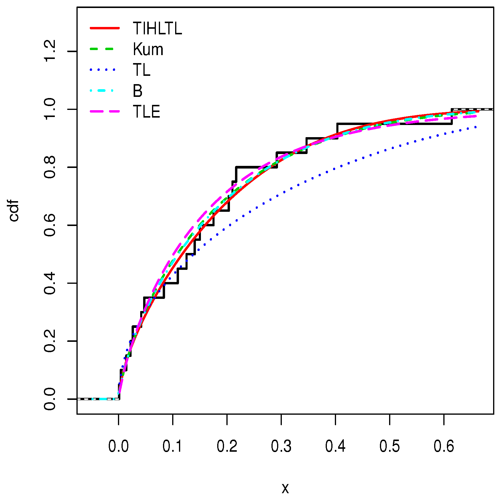
The first data set. We considered the data from [30] about theordered failure of components. The data are given as follows:

0.0009, 0.004, 0.0142, 0.0221, 0.0261, 0.0418, 0.0473, 0.0834, 0.1091, 0.1252, 0.1404, 0.1498, 0.175, 0.2031, 0.2099, 0.2168, 0.2918, 0.3465, 0.4035, 0.6143

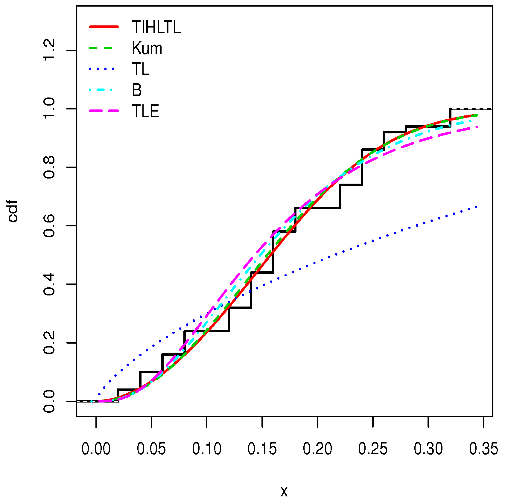
The second data set. The second data set refers to 50 observations on burr (in millimeters), with hole diameter and sheet thickness of 12 mm and 3.15 mm, respectively. We refer to [31] for the technical details behind these measures. The data are given as follows:

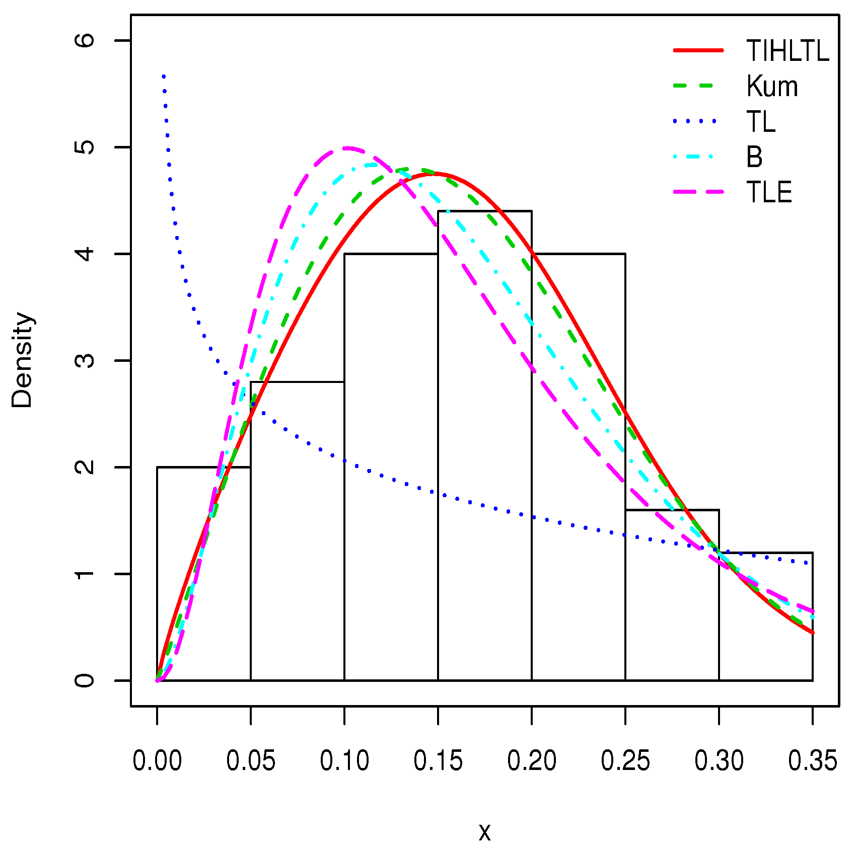
0.04, 0.02, 0.06, 0.12, 0.14, 0.08, 0.22, 0.12, 0.08, 0.26, 0.24, 0.04, 0.14, 0.16, 0.08, 0.26, 0.32, 0.28, 0.14, 0.16, 0.24, 0.22, 0.12, 0.18, 0.24, 0.32, 0.16, 0.14, 0.08, 0.16, 0.24, 0.16, 0.32, 0.18, 0.24, 0.22, 0.16, 0.12, 0.24, 0.06, 0.02, 0.18, 0.22, 0.14, 0.06, 0.04, 0.14, 0.26, 0.18, 0.16

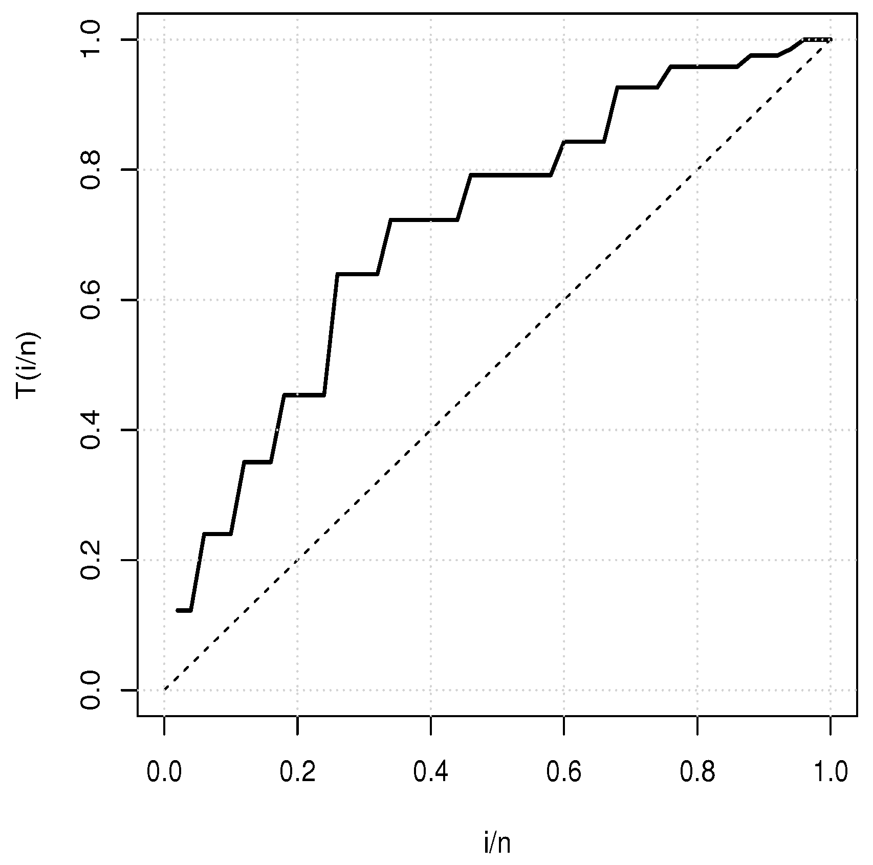
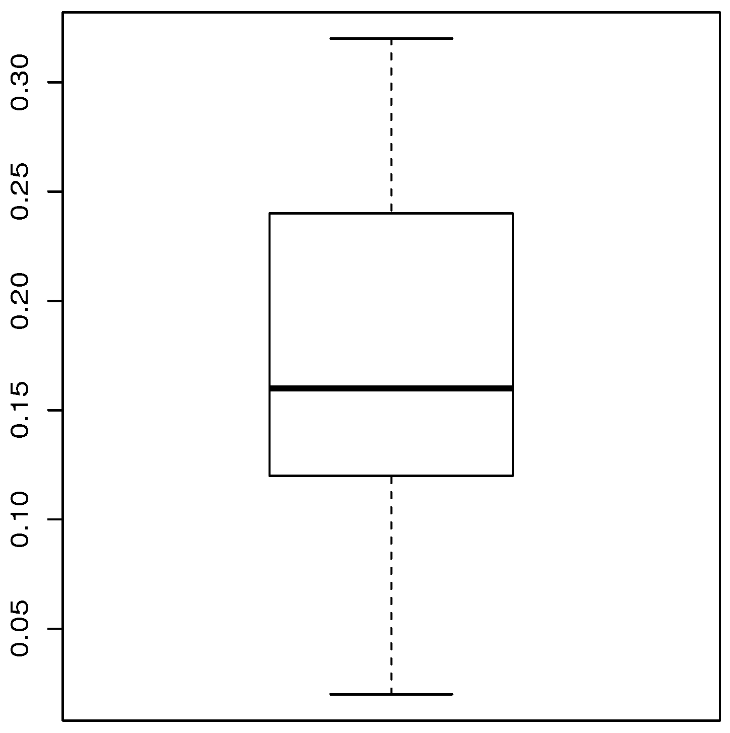
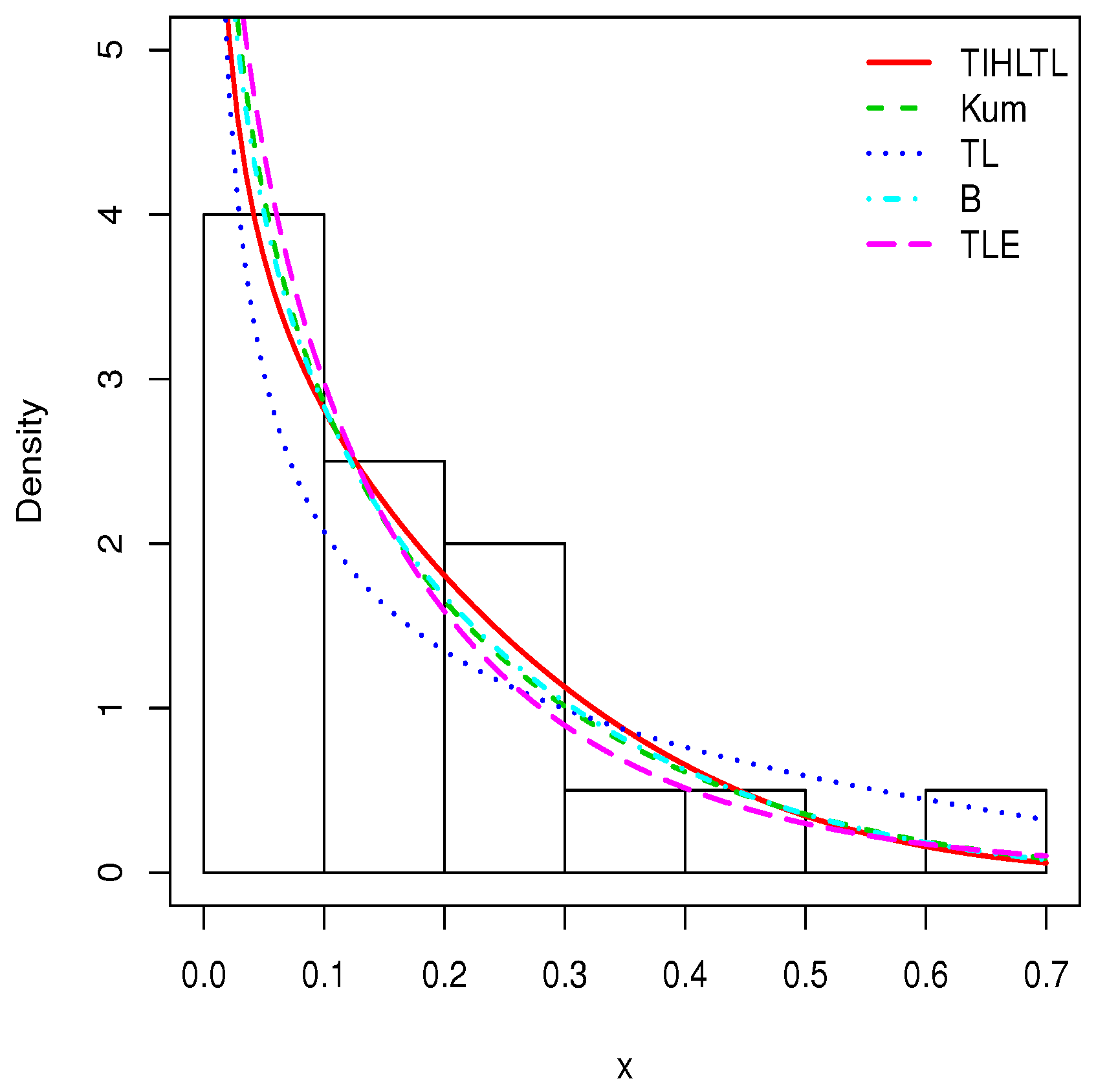
Table 8 provides a basic statistical description of the two data sets. One can remark that data set 1 is highly right skewed, contrary to data set 2. Figure 5 and Figure 6 show the total test time (TTT) plots for data sets 1 and 2, respectively. In particular, the observed curves in the TTT plots are (more or less) concave, implying that a (more or less) monotonic hrf is adequate, giving first signs that the TIHLTL model is appropriate for such data. For more detail on the TTT plot, see [32]. As a complement to this, Figure 7 and Figure 8 present the boxplots for data sets 1 and 2, respectively. The MLEs of the considered models along with their standard errors are given in Table 9 and Table 10 for data sets 1 and 2, respectively. Table 11 and Table 12 contain the values of the goodness-of-fit measures for the considered models. Plots of the estimated pdfs corresponding to data sets 1 and 2 can be observed in Figure 9 and Figure 10, respectively. Plots of the estimated cdfs corresponding to data sets 1 and 2 can be observed in Figure 11 and Figure 12, respectively. Finally, confidence intervals (CIs) for the TIHLTL model parameters are given in Table 13.

Table 8. First statistical approach of data sets 1 and 2.

	n	Mean	Median	Standard Deviation	Skewness	Kurtosis
Data set 1	20	0.16	0.13	0.16	1.23	1.07
Data set 2	50	0.16	0.16	0.08	0.07	−0.87

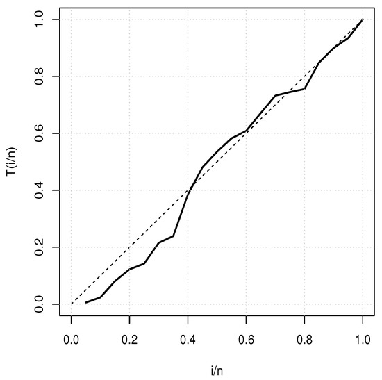
Figure 5. TTT plot for data set 1.

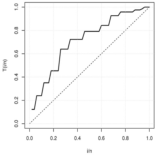
Figure 6. TTT plot for data set 2.

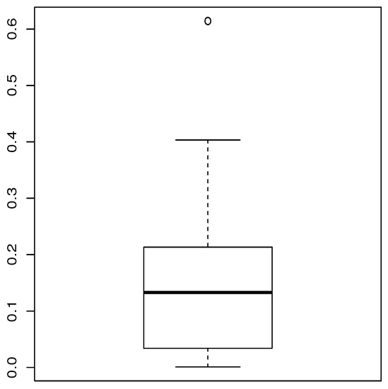
Figure 7. Boxplot for data set 1.

Figure 8. Boxplot for data set 2.

Table 9. MLEs and their standard errors (in parentheses) for data set 1. B: beta model; Kum: Kumaraswamy model. TL: Topp–Leone model; TLE: Topp–Leone exponential model.

Model	λ	α	a	b
TIHLTL	2.1342	0.6028	-	-
	(0.6336)	(0.1706)	-	-
Kum	-	-	0.7639	3.4341
	-	-	(0.1751)	(1.3113)
TL	-	0.5112	-	-
	-	(0.1143)	-	-
B	-	-	0.7134	3.7459
	-	-	(0.1931)	( 1.3085)
TLE	0.7925	2.6644	-	-
	(0.2208)	(0.8240)	-	-

Table 10. MLEs along with their standard errors (in parentheses) for data set 2.

Model	λ	α	a	b
TIHLTL	10.6094	1.8752	-	-
	(1.1160)	(0.2643)	-	-
Kum	-	-	2.0750	33.0041
	-	-	(0.2542)	(3.8351)
TL	-	0.7247	-	-
	-	(0.1024)	-	-
B	-	-	2.6799	13.8502
	-	-	(0.5066)	(2.8249)
TLE	3.1718	5.6800	-	-
	(0.7067)	(0.7841)	-	-

Table 11. Statistical measures for data set 1. A*: Anderson–Darling criterion; AIC: Akaike Information Criterion; BIC: Bayesian Information Criterion; KS: Kolmogorov–Smirnov statistic; W*: Cramer–von Mises criterion.

Model	$-\widehat{\mathit{\ell }}$	AIC	BIC	W*	A*	KS	p-Value (KS)
TIHLTL	−17.3028	−30.6057	−28.6143	0.0208	0.1348	0.0900	0.9912
Kum	−17.2047	−30.4094	−28.4180	0.0289	0.1691	0.1026	0.9700
TL	−15.6166	−29.2333	−28.2376	0.0300	0.1754	0.1848	0.4481
B	−17.2532	−30.5064	−28.5150	0.0263	0.1565	0.0980	0.9782
TLE	−16.8608	−29.7216	−27.7301	0.0375	0.2124	0.1225	0.8899

Table 12. Statistical measures for data set 2.

Model	$-\widehat{\mathit{\ell }}$	AIC	BIC	W*	A*	KS	p-Value (KS)
TIHLTL	−56.4261	−108.8522	−105.0282	0.0893	0.5496	0.1031	0.6623
Kum	−56.0686	−108.1373	−104.3132	0.1024	0.6248	0.1104	0.5755
TL	−28.4078	−54.8156	−52.9035	0.1653	0.9919	0.3622	0.000003
B	−54.6066	−105.2133	−101.3892	0.1479	0.8926	0.1414	0.2697
TLE	−52.2862	−100.5725	−96.7484	0.2120	1.2634	0.1652	0.1302

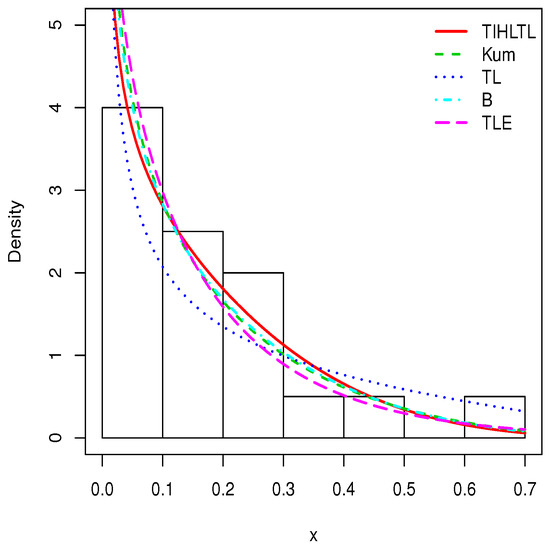
Figure 9. Plots of estimated probability density functions (pdfs) for data set 1.

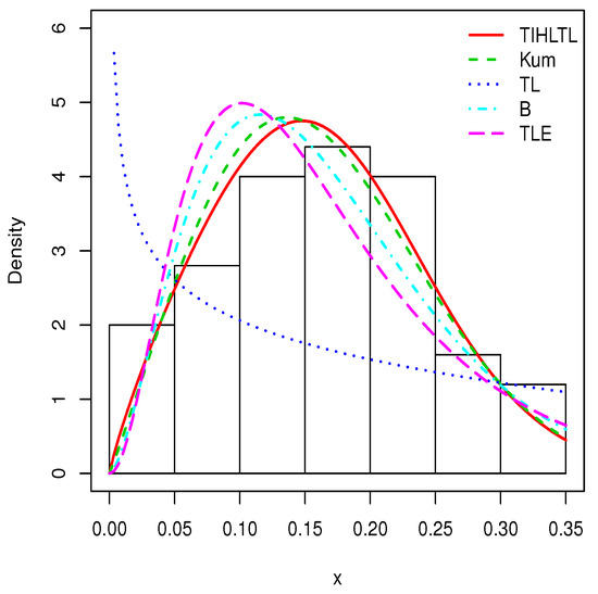
Figure 10. Plots of estimated probability density functions (pdfs) for data set 2.

Figure 11. Plots of estimated cumulative distribution functions (cdfs) for data set 1.

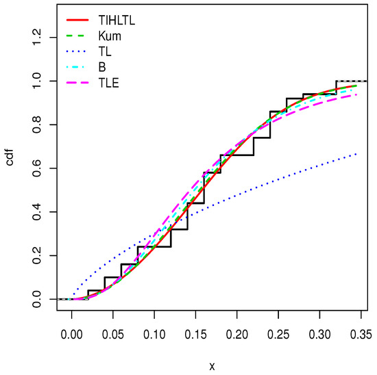
Figure 12. Plots of estimated cumulative distribution functions (cdfs) for data set 2.

Table 13. Confidence intervals of the TIHLTL model parameters for data sets 1 and 2, respectively.

CI	λ	α
95%	[0.8923 3.3760]	[0.2684 0.9371]
99%	[0.4995 3.7688]	[0.1626 1.0429]
CI	λ	α
95%	[8.4220 12.7967]	[1.3571 2.3932]
99%	[7.7301 13.4886]	[1.1933 2.5570]

From Table 11 and Table 12, we observe that the AIC, BIC, A*, and W* of the TIHLTL model had minimum values compared to the other competitive models, so we conclude that the TIHLTL model provided the best fit on these data sets. Figure 9, Figure 11, Figure 10 and Figure 12 support this claim.

6. Concluding Remarks

In this paper, we studied a special member of the type I half-logistic-G family based on the Topp–Leone distribution, constituting a new two-parameter continuous distribution with support in $(0,1)$, called the TIHLTL distribution. Among its advantages, a wide variety of shapes are observed for the corresponding pdf and hrf. Some properties of the TIHLTL distribution, such as asymptotes, shapes, quantile function, skewness, kurtosis, some power series expansions, ordinary moments, incomplete moments, moment-generating function, stress strength parameter, and order statistics, were derived. Then, the statistical aspects of the TIHLTL model were explored, assuming that the parameters $\lambda$ and $\alpha$ were unknown. A simulation study was performed to compare the model performance of seven well-established estimation methods. An application of the TIHLTL model to two practical data sets showed that it is a serious competitor to other well-established models, such as the beta and Kumaraswamy models.

References

- Gupta, R.D.; Kundu, D. Exponentiated exponential family: An alternative to Gamma and Weibull distributions. Biom. J. 2001, 43, 117–130. [Google Scholar] [CrossRef]
- Eugene, N.; Lee, C.; Famoye, F. Beta-normal distribution and its applications. Commun. Stat.-Theory Methods 2002, 31, 497–512. [Google Scholar] [CrossRef]
- Zografos, K.; Balakrishnan, N. On families of beta- and generalized gamma-generated distributions and associated inference. Stat. Methodol. 2009, 6, 344–362. [Google Scholar] [CrossRef]
- Alizadeh, M.; Emadiz, M.; Doostparast, M.; Cordeiro, G.M.; Ortega, E.M.M.; Pescim, R.R. A new family of distributions: The Kumaraswamy odd log-logistic, properties and applications. Hacet. J. Math. Stat. 2015, 44, 1491–1512. [Google Scholar] [CrossRef]
- Cordeiro, G.M.; Alizadeh, M.; Marinho, E.P.R.D. The type I half-logistic family of distributions. J. Stat. Comput. Simul. 2015, 86, 707–728. [Google Scholar] [CrossRef]
- Cordeiro, G.M.; Alizadeh, M.; Ozel, G. The generalized odd log-logistic family of distributions: Properties, regression models and applications. J. Stat. Comput. Simul. 2017, 87, 908–932. [Google Scholar] [CrossRef]
- Alizadeh, M.; Altun, E.; Cordeiro, G.M.; Rasekhi, M. The odd power Cauchy family of distributions: Properties, regression models and applications. J. Stat. Comput. Simul. 2018, 88, 785–805. [Google Scholar] [CrossRef]
- Reyad, H.M.; Alizadeh, M.; Jamal, F.; Othman, S.; Hamedani, G.G. The Exponentiated Generalized Topp Leone-G Family of Distributions: Properties and Applications. Pak. J. Stat. Oper. Res. 2019, 15, 1–24. [Google Scholar] [CrossRef]
- Jamal, F.; Chesneau, C.; Elgarhy, M. Type II general inverse exponential family of distributions. J. Stat. Manag. Syst. 2019. Available online: https://www.tandfonline.com/toc/tsms20/current (accessed on 15 August 2019).
- Topp, C.W.; Leone, F.C. A family of J-shaped frequency functions. J. Am. Stat. Assoc. 1955, 50, 209–219. [Google Scholar] [CrossRef]
- Nadarajah, S.; Kotz, S. Moments of some J-shaped distributions. J. Appl. Stat. 2003, 30, 311–317. [Google Scholar] [CrossRef]
- Ghitany, M.E.; Kotz, S.; Xie, M. On some reliability measures and their stochastic orderings for the Topp-Leone distribution. J. Appl. Stat. 2005, 32, 715–722. [Google Scholar] [CrossRef]
- Sangsanit, Y.; Bodhisuwan, W. The Topp-Leone generator of distributions: Properties and inferences. Songklanakarin J. Sci. Technol. 2016, 38, 537–548. [Google Scholar]
- Kunjiratanachot, N.; Bodhisuwan, W.; Volodin, A. The Topp-Leone generalized exponential power series distribution with applications. J. Probab. Stat. Sci. 2018, 16, 197–208. [Google Scholar]
- Elgarhy, M.; Nasir, M.A.; Jamal, F.; Ozel, G. The type II Topp-Leone generated family of distributions: Properties and applications. J. Stat. Manag. Syst. 2018, 21, 1529–1551. [Google Scholar] [CrossRef]
- Mauldon, J.M. A Generalization of the Beta-distribution. Ann. Math. Stat. 1959, 30, 509–520. [Google Scholar] [CrossRef]
- Kumaraswamy, P. A generalized probability density function for double-bounded random processes. J. Hydrol. 1980, 46, 79–88. [Google Scholar] [CrossRef]
- Abramowitz, M.; Stegun, I.A. Handbook of Mathematical Functions, National Bureau of Standards; Applied Math. Series 55; Dover Publications: Mineola, NY, USA, 1965. [Google Scholar]
- Galton, F. Inquiries Into Human Faculty and Its Development; Macmillan and Company: London, UK, 1883. [Google Scholar]
- Moors, J.J.A. A quantile alternative for Kurtosis. J. R. Stat. Soc. Ser. D (Stat.) 1988, 37, 25–32. [Google Scholar] [CrossRef]
- Kotz, S.; Lumelskii, Y.; Penskey, M. The Stress-Strength Model and Its Generalizations and Applications; World Scientific: Singapore, 2003. [Google Scholar]
- David, H.A.; Nagaraja, H.N. Order Statistics; John Wiley and Sons: Hoboken, NJ, USA, 2003. [Google Scholar]
- Casella, G.; Berger, R.L. Statistical Inference; Brooks/Cole Publishing Company: Bel Air, CA, USA, 1990. [Google Scholar]
- Swain, J.J.; Venkatraman, S.; Wilson, J.R. Least-squares estimation of distribution functions in johnson’s translation system. J. Stat. Comput. Simul. 1988, 29, 271–297. [Google Scholar] [CrossRef]
- Macdonald, P.D.M. Comment on ‘An estimation procedure for mixtures of distributions’ by Choi and Bulgren. J. R. Stat. Soc. B 1971, 33, 326–329. [Google Scholar]
- Kao, J. Computer methods for estimating Weibull parameters in reliability studies. IRE Trans. Reliab. Qual. Control 1958, 13, 15–22. [Google Scholar] [CrossRef]
- Kao, J. A graphical estimation of mixed Weibull parameters in life testing electron tube. Technometrics 1959, 1, 389–407. [Google Scholar] [CrossRef]
- Anderson, T.W.; Darling, D.A. Asymptotic theory of certain ‘goodness-of- fit’ criteria based on stochastic processes. Ann. Math. Stat. 1952, 23, 193–212. [Google Scholar] [CrossRef]
- Al-Shomrani, A.; Arif, O.; Shawky, K.; Hanif, S.; Shahbaz, M.Q. Topp-Leone family of distributions: Some properties and application. Pak. J. Stat. Oper. Res. 2016, 12, 443–451. [Google Scholar] [CrossRef]
- Nigm, A.M.; AL-Hussaini, E.K.; Jaheen, Z.F. Bayesian one sample prediction of future observations under Pareto distribution. Statistics 2003, 37, 527–536. [Google Scholar] [CrossRef]
- Dasgupta, R. On the distribution of Burr with applications. Sankhya 2011, 73, 1–19. [Google Scholar] [CrossRef]
- Aarset, M.V. How to identify bathtub hazard rate. IEEE Trans. Reliab. 1987, 36, 106–108. [Google Scholar] [CrossRef]
© 2019 by the authors. Licensee MDPI, Basel, Switzerland. This article is an open access article distributed under the terms and conditions of the Creative Commons Attribution (CC BY) license (http://creativecommons.org/licenses/by/4.0/).