Identification of Source Term for the Time-Fractional Diffusion-Wave Equation by Fractional Tikhonov Method

Abstract

In this article, we consider an inverse problem to determine an unknown source term in a space-time-fractional diffusion equation. The inverse problems are often ill-posed. By an example, we show that this problem is NOT well-posed in the Hadamard sense, i.e., this problem does not satisfy the last condition-the solution’s behavior changes continuously with the input data. It leads to having a regularization model for this problem. We use the Tikhonov method to solve the problem. In the theoretical results, we also propose a priori and a posteriori parameter choice rules and analyze them.

1. Introduction

Let $\mathsf{\Omega }$ be a bounded domain in ${\mathbb{R}}^d$ with sufficiently smooth boundary $\partial \mathsf{\Omega }$, $\beta \in (1,2)$. In this paper, we consider the inverse source problem of the time-fractional diffusion-wave equation:

$$\begin{array}{c}\hfill \left\{\begin{array}{cc}{\partial }_{0^{+}}^{\beta }u(x,t)=\Delta u(x,t)+\mathsf{\Xi }\left(x\right),\hfill & (x,t)\in \mathsf{\Omega }\times (0,T),\hfill \\ u(x,t)=0,\hfill & (x,t)\in \partial \mathsf{\Omega }\times (0,T],\hfill \\ u(x,0)=f\left(x\right),\hfill & x\in \mathsf{\Omega },\hfill \\ u_t(x,0)=g\left(x\right),\hfill & x\in \mathsf{\Omega },\hfill \\ u(x,T)=h\left(x\right),\hfill & x\in \mathsf{\Omega },\hfill \end{array}\right.\end{array}$$

(1)

where ${\partial }_{0^{+}}^{\beta }u(x,t)$ is the Caputo fractional derivative of order $\beta$ defined as [1]

$$\begin{array}{c}\hfill {\partial }_{0^{+}}^{\beta }u(x,t)=\frac{1}{\Gamma (2-\alpha )}{\int }_0^t\frac{{\partial }^{2}u(x,s)}{\partial s^2}\frac{ds}{{(t-s)}^{\beta -1}},1<\beta <2,\end{array}$$

(2)

where $\Gamma (.)$ is the Gamma function.

It is known that the inverse source problem mentioned above is ill-posed in general, i.e., a solution does not always exist and, in the case of existence of a solution, it does not depend continuously on the given data. In fact, from a small noise of physical measurement, for example, $(h,f,g)$ is noised by observation data $(h^{{\epsilon }_1},g^{{\epsilon }_2},h^{{\epsilon }_3})$ with order of ${\epsilon }_1>0,{\epsilon }_2>0$, and ${\epsilon }_3>0$.

$$\begin{array}{c}\hfill \Vert h-h^{{\epsilon }_1}{\Vert }_{{\mathcal{L}}^2\left(\mathsf{\Omega }\right)}\le {\epsilon }_1,\Vert f-f^{{\epsilon }_2}{\Vert }_{{\mathcal{L}}^2\left(\mathsf{\Omega }\right)}\le {\epsilon }_2,\mathrm{and}\Vert g-g^{{\epsilon }_3}{\Vert }_{{\mathcal{L}}^2\left(\mathsf{\Omega }\right)}\le {\epsilon }_3.\end{array}$$

(3)

In all functions $f\left(x\right)$, $g\left(x\right)$, and $h\left(x\right)$ are given data. It is well-known that if ${\epsilon }_1,{\epsilon }_2,\mathrm{and}{\epsilon }_3$ are small enough, the sought solution $\mathsf{\Xi }\left(x\right)$ may have a large error. The backward problem is to find $\mathsf{\Xi }\left(x\right)$ from ${\mathsf{\Xi }}^{\mathbf{\epsilon }}$ and $g^{\mathbf{\epsilon }}$ which satisfies (3), where ${\Vert ·\Vert }_{{\mathcal{L}}^2\left(\mathsf{\Omega }\right)}$ denotes the ${\mathcal{L}}^2$ norm.

It is known that the inverse source problem mentioned above is ill-posed in general, i.e., a solution does not always exist, and in the case of existence of a solution, it does not depend continuously on the given data. In fact, from a small noise of physical measurement, the corresponding solutions may have a large error. Hence, a regularization is required. Inverse source problems for a time-fractional diffusion equation for $0<\beta <1$ have been studied. Tuan et al. [2] used the Tikhonov regularization method to solve the inverse source problem with the later time and show the estimation for the exact solution and regularized solution by a priori and a posteriori parameter choices rules. Wei et al. [3,4,5] studied an inverse source problem in a spatial fractional diffusion equation by quasi-boundary value and truncation methods. Fan Yang et al., see [6], used the Landweber iteration regularization method for determining the unknown source for the modified Helmholtz equation. Nevertheless, to our best knowledge, Salir Tarta et al. [7] used these properties and analytic Fredholm theorem to prove that the inverse source problem is well-posed, i.e., $f(t,x)$ can be determined uniquely and depends continuously on additional data $u(T,x)$, $x\in \mathsf{\Omega }$, see [8,9]—the authors studied the inverse source problem in the case of nonlocal inverse problem in a one-dimensional time-space and numerical algorithm. Furthermore, the research of backward problems for the diffusion-wave equation is an open problem and still receives attention. In 2017, Tuan et al. [10] considered

$$\left\{\begin{array}{cc}{\displaystyle \frac{{\partial }^{\beta }}{\partial t^{\beta }}}u(x,t)=-r^{\beta }{(-\Delta )}^{\frac{\alpha }{2}}u(x,t)+h\left(t\right)f\left(x\right),\hfill & (x,t)\in {\mathsf{\Omega }}_T,\hfill \\ u(-1,t)=u(1,t)=0,\hfill & 0<t<T,\hfill \\ u(x,0)=0,\hfill & x\in \mathsf{\Omega },\hfill \\ u(x,T)=g\left(x\right),\hfill & x\in \mathsf{\Omega },\hfill \end{array}\right.$$

(4)

where ${\mathsf{\Omega }}_T=(-1,1)\times (0,T)$; $r>0$ is a parameter; $h\in C[0,T]$ is a given function; $\beta \in (0,1)$; $\alpha \in (1,2)$ are fractional order of the time and the space derivatives, respectively; and $T>0$ is a final time. The function $u=u(x,t)$ denotes a concentration of contaminant at a position x and time t with ${(-\Delta )}^{\frac{\alpha }{2}}$ as the fractional Laplacian. If $\alpha$ tends to 2, the fractional Laplacian tends to the Laplacian normal operator, see [1,2,7,8,9,10,11,12,13,14,15,16]. In this paper, we use the fractional Tikhonov regularization method to solve the identification of source term of the fractional diffusion-wave equation inverse source problem with variable coefficients in a general bounded domain. However, a fractional Tikhonov is not a new method for mathematicians in the world. In [16], Zhi Quan and Xiao Li Feng used this method for considering the Helmholtz equation. Here, we estimate a convergence rate under an a priori bound assumption of the exact solution and a priori parameter choice rule and estimate a convergence rate under the a posteriori parameter choice rule.

In several papers, many authors have shown that the fractional diffusion-wave equation plays a very important role in describing physical phenomena, such as the diffusion process in media with fractional geometry, see [17]. Nowadays, fractional calculus receives increasing attention in the scientific community, with a growing number of applications in physics, electrochemistry, biophysics, viscoelasticity, biomedicine, control theory, signal processing, etc., see [18]. In a lot of papers, the Mittag–Leffler function and its properties are researched and the results are used to model the different physical phenomena, see [19,20].

The rest of this article is organized as follows. In Section 2, we introduce some preliminary results. The ill-posedness of the fractional inverse source problem (1) and conditional stability are provided in Section 3. We propose a Tikhonov regularization method and give two convergence estimates under an a priori assumption for the exact solution and two regularization parameter choice rules: Section 4 (a priori parameter choice) and Section 5 (a posteriori parameter choice).

2. Preliminary Results

In this section, we introduce a few properties of the eigenvalues of the operator $(-\Delta )$, see [21].

Definition 1

(Eigenvalues of the Laplacian operator).

1. 

Each eigenvalues of $(-\Delta )$ is real. The family of eigenvalues ${\left\{{\tilde{b}}_i\right\}}_{i=1}^{\infty }$ satisfy $0\le {\tilde{b}}_1\le {\tilde{b}}_2\le {\tilde{b}}_3\le \cdots$, and ${\tilde{b}}_i\to \infty$ as $i\to \infty$.

2. 

We take $\{{\tilde{b}}_i,{\mathrm{e}}_i\}$ the eigenvalues and corresponding eigenvectors of the fractional Laplacian operator in Ω with Dirichlet boundary conditions on $\partial \mathsf{\Omega }$:

$$\begin{array}{c}-\Delta {\mathrm{e}}_i\left(x\right)={\tilde{b}}_i{\mathrm{e}}_i\left(x\right),x\in \mathsf{\Omega },\\ {\mathrm{e}}_i\left(x\right)=0,\mathrm{on}\partial \mathsf{\Omega },\end{array}$$

(5)

for $i=1,2,\cdots$. Then, we define the operator $(-\Delta )$ by

$$\begin{array}{c}\hfill -\Delta u:=\sum _{i=0}^{\infty }{c}_i(-\Delta {\mathrm{e}}_i\left(x\right))=\sum _{i=0}^{\infty }{c}_i{\tilde{b}}_i{\mathrm{e}}_i\left(x\right),\end{array}$$

(6)

which maps $H_0^{\kappa }\left(\mathsf{\Omega }\right)$ into ${\mathcal{L}}_2\left(\mathsf{\Omega }\right)$. Let $0\ne \kappa <\infty$. By $H^{\kappa }\left(\mathsf{\Omega }\right)$, we denote the space of all functions $g\in {\mathcal{L}}_2\left(\mathsf{\Omega }\right)$ with the property

$$\sum _{i=1}^{\infty }{(1+{\tilde{b}}_i)}^{2\kappa }|g_i{|}^2<\infty ,$$

(7)

where $g_i={\int }_{\mathsf{\Omega }}g\left(x\right){\mathrm{e}}_i\left(x\right)dx.$ Then, we also define $\Vert g{\Vert }_{H^{\kappa }\left(\mathsf{\Omega }\right)}=\sqrt{{\sum }_{i=1}^{\infty }{(1+{\tilde{b}}_i)}^{2\kappa }|g_i{|}^2}$. If $\kappa =0$, then $H^{\kappa }\left(\mathsf{\Omega }\right)$ is ${\mathcal{L}}_2\left(\mathsf{\Omega }\right).$

Definition 2

(See [1]). The Mittag–Leffler function is:

$$\begin{array}{c}\hfill E_{\beta ,\gamma }\left(z\right)=\sum _{i=0}^{\infty }\frac{z^i}{\Gamma (\beta i+\gamma )},z\in \mathbb{C},\end{array}$$

where $\beta >0$ and $\gamma \in \mathbb{R}$ are arbitrary constants.

Lemma 1

(See [21]). For $1<\beta <2$, $\gamma \in \mathbb{R}$, and $\omega >0$, we get

$$\begin{array}{c}\hfill E_{\beta ,\gamma }(-\omega )=\frac{1}{\Gamma (\gamma -\beta )\omega }+o\left(\frac{1}{{\omega }^2}\right),\omega \to \infty ·\end{array}$$

(8)

Lemma 2

(See [1]). If $\beta <2$ and $\gamma \in \mathbb{R}$, suppose ζ satisfies ${\displaystyle \frac{\pi \beta }{2}}<\zeta <min\{\pi ,\pi \beta \}$, $\zeta \le |arg(y)|\le \pi$. Then, there exists a constant $\tilde{A}$ as follows:

$$\begin{array}{c}\hfill |E_{\beta ,\gamma }\left(y\right)|\le {\displaystyle \frac{\tilde{A}}{1+|y|}}·\end{array}$$

(9)

Lemma 3

(See [22]). The following equality holds for $\tilde{b}>0$, $\alpha >0$ and $m\in \mathbb{N}$

$$\frac{d^m}{d{t}^m}{E}_{\alpha ,1}(-\tilde{b}{t}^{\alpha })=-\tilde{b}{t}^{\alpha -m}{E}_{\alpha ,\alpha -m+1}(-\tilde{b}{t}^{\alpha }),t>0.$$

(10)

Lemma 4.

For ${\tilde{b}}_i>0$, $\beta >0$, and positive integer $i\in \mathbb{N}$, we have

$$\begin{array}{cc}\hfill & \left(1\right)\frac{d}{dt}\left(t{E}_{\beta ,2}\left({\tilde{b}}_i{t}^{\beta }\right)\right)=E_{\beta ,1}(-{\tilde{b}}_i{t}^{\beta }),\hfill \\ \hfill & \left(2\right)\frac{d}{dt}\left(E_{\beta ,1}(-{\tilde{b}}_i{t}^{\beta })\right)=-{\tilde{b}}_i{t}^{\beta -1}{E}_{\beta ,\beta }(-{\tilde{b}}_i{t}^{\beta }).\hfill \end{array}$$

(11)

Lemma 5.

For any ${\tilde{b}}_i$ satisfying ${\tilde{b}}_i\ge {\tilde{b}}_1>0$, there exists positive constants $A,B$ such that

$$\begin{array}{c}\hfill \frac{A}{{\tilde{b}}_i{T}^{\beta }}\le |E_{\beta ,\beta +1}\left(-{\tilde{b}}_i{T}^{\beta }\right)|\le \frac{B}{{\tilde{b}}_i{T}^{\beta }}·\end{array}$$

(12)

Lemma 6

(See [21]). Let $\tilde{b}>0$, we have

$$\begin{array}{c}\hfill \underset{0}{\overset{\infty }{\int }}{e}^{-pt}{t}^{\beta i+\gamma -1}{E}_{\beta ,\gamma }^{\left(i\right)}(\pm a{t}^{\beta })dt=\frac{i!p^{\beta -\gamma }}{{(p^{\beta }\mp a)}^{i+1}},\Re \left(a\right)>{\Vert a\Vert }^{\frac{1}{\beta }},\end{array}$$

(13)

where $E_{\beta ,\gamma }^{\left(i\right)}\left(y\right):=\frac{d^i}{d{y}^i}{E}_{\beta ,\gamma }\left(y\right).$

Lemma 7.

For constant $\xi \ge {\tilde{b}}_1$ and ${\displaystyle \frac{1}{2}}\le \tau \le 1$, one has

$$\begin{array}{c}\hfill \mathcal{C}\left(\xi \right)={\displaystyle \frac{\xi }{A^{2\tau }+{\alpha }^2{\xi }^{2\tau }}}\le \overline{C}(\tau ,A){\alpha }^{-\frac{1}{\tau }},\end{array}$$

(14)

where $\overline{C}=\overline{C}(\tau ,A)$ are independent on $\alpha ,\xi$.

Proof. 

Let ${\displaystyle \frac{1}{2}}\le \tau \le 1$, we solve the equation ${\mathcal{C}}^{\prime }\left({\xi }_0\right)=0$, then there exists a unique ${\xi }_0=A{(2\tau -1)}^{-\frac{1}{2\tau }}{\alpha }^{-\frac{1}{\tau }}$, it gives

$$\begin{array}{c}\hfill \mathcal{C}\left(\xi \right)\le \mathcal{C}\left({\xi }_0\right)\le \frac{A^{1-2\tau }}{2\tau }{(2\tau -1)}^{\frac{2\tau -1}{2\tau }}{\alpha }^{-\frac{1}{\tau }}:=\overline{C}(\tau ,A){\alpha }^{-\frac{1}{\tau }}.\end{array}$$

 □

Lemma 8.

Let the constant $\xi \ge {\tilde{b}}_1$ and $\frac{1}{2}\le \tau \le 1$, we get

$$\begin{array}{c}\hfill \mathcal{D}\left(\xi \right)={\displaystyle \frac{{\alpha }^2{\xi }^{2\tau -j}}{A^{2\tau }+{\alpha }^2{\xi }^{2\tau }}}\le \left\{\begin{array}{c}{\mathcal{B}}_1(j,\tau ,A){\alpha }^{\frac{j}{\tau }},0<j<2\tau ,\hfill \\ {\mathcal{B}}_2(j,\tau ,A,{\tilde{b}}_1){\alpha }^2,j\ge 2\tau .\hfill \end{array}\right.\end{array}$$

Proof. 

• If $j\ge 2\tau$, then from $\xi \ge {\tilde{b}}_1$, we get

  $$\begin{array}{c}\hfill \mathcal{D}\left(\xi \right)=\frac{{\alpha }^2{\xi }^{2\tau -j}}{A^{2\tau }+{\alpha }^2{\xi }^{2\tau }}\le \frac{{\alpha }^2{\xi }^{2\tau -j}}{A^{2\tau }}\le \frac{{\alpha }^2}{A^{2\tau }{\tilde{b}}_1^{j-2\tau }}\le \frac{1}{A^{2\tau }{\tilde{b}}_1^{j-2\tau }}{\alpha }^2.\end{array}$$

  (15)
• If $0<j<2\tau$, then it can be seen that ${lim}_{\xi \to 0}\mathcal{D}\left(\xi \right)={lim}_{\xi \to +\infty }\mathcal{D}\left(\xi \right)=0.$ Taking the derivative of $\mathcal{D}$ with respect to $\xi$, we know that

  $$\begin{array}{c}\hfill {\mathcal{D}}^{\prime }\left(\xi \right)=\frac{{\alpha }^2(2\tau -j){\xi }^{2\tau -j-1}(A^{2\tau }+{\alpha }^2{\xi }^{2\tau })-{\alpha }^{4}2\tau {\xi }^{4\tau -j-1}}{{(A^{2\tau }+{\alpha }^2{\xi }^{2\tau })}^2}·\end{array}$$

  (16)

From (16), a simple transformation gives

$$\begin{array}{c}\hfill {\mathcal{D}}^{\prime }\left(\xi \right)=\frac{{\alpha }^2(2\tau -j)A^{2\tau }{\xi }^{2\tau -j-1}-{\alpha }^{4}j{\xi }^{4\tau -j-1}}{{(A^{2\tau }+{\alpha }^2{\xi }^{2\tau })}^2}·\end{array}$$

(17)

$\mathcal{D}\left(\xi \right)$ attains maximum value at $\xi ={\xi }_0$ such that it satisfies ${\mathcal{D}}^{\prime }\left(\xi \right)=0$. Solving ${\mathcal{D}}^{\prime }\left({\xi }_0\right)=0$, we know that ${\xi }_0=A{(2\tau -j)}^{\frac{1}{2\tau }}{\alpha }^{-\frac{1}{\tau }}{j}^{-\frac{1}{2\tau }}$.

Hence, we conclude

$$\begin{array}{c}\hfill \mathcal{D}\left(\xi \right)\le \mathcal{D}\left({\xi }_0\right)=\mathcal{D}\left(A{(2\tau -j)}^{\frac{1}{2\tau }}{\alpha }^{-\frac{1}{\tau }}{j}^{-\frac{1}{2\tau }}\right)=\frac{{(2\tau -j)}^{\frac{2\tau -j}{2\tau }}{A}^{-j}{j}^{\frac{j}{2\tau }}}{2\tau }{\alpha }^{\frac{j}{\tau }}.\end{array}$$

(18)

 □

Lemma 9.

Let $\xi >{\tilde{b}}_1>0$ and $\frac{1}{2}\le \tau <1$, and $\mathcal{F}\left(\xi \right)$ be a function defined by

$$\begin{array}{c}\hfill \mathcal{F}\left(\xi \right)={\displaystyle \frac{{\alpha }^2{\xi }^{2\tau -(j+1)}}{A^{2\tau }+{\alpha }^2{\xi }^{2\tau }}}\le \left\{\begin{array}{c}{\mathcal{B}}_3(j,\tau ,A){\alpha }^{\frac{j+1}{\tau }},0<j<2\tau -1,\hfill \\ {\mathcal{B}}_4(j,\tau ,A,{\tilde{b}}_1){\alpha }^2,j\ge 2\tau -1,\hfill \end{array}\right.\end{array}$$

where ${\mathcal{B}}_3(j,\tau ,A,{\tilde{b}}_1)={\displaystyle \frac{2\tau -j-1}{2\tau A^{2\tau }}}{\left({\displaystyle \frac{j+1}{2\tau -j-1}}\right)}^{\frac{j+1}{2\tau }}$ and ${\mathcal{B}}_4(j,\tau ,A,{\tilde{b}}_1)={\displaystyle \frac{1}{A^{2\tau }{\tilde{b}}_1^{(j+1)-2\tau }}}$.

Proof. 

• If $j\ge 2\tau -1$, then for $\xi \ge {\tilde{b}}_1$ we know that

  $$\begin{array}{c}\hfill \mathcal{F}\left(\xi \right)\le \frac{{\alpha }^2{\xi }^{2\tau -(j+1)}}{A^{2\tau }}\le \frac{1}{A^{2\tau }{\tilde{b}}_1^{(j+1)-2\tau }}{\alpha }^2={\mathcal{B}}_4(j,\tau ,A,{\tilde{b}}_1){\alpha }^2.\end{array}$$

  (19)
• If $0<j<2\tau -1$, then we have ${lim}_{\xi \to 0}\mathcal{F}\left(\xi \right)={lim}_{\xi \to \infty }\mathcal{F}\left(\xi \right)=0$, then we know

  $$\begin{array}{c}\hfill \mathcal{F}\left(\xi \right)\le \underset{\xi \in (0,+\infty )}{sup}\mathcal{F}\left(\xi \right)\le \mathcal{F}\left({\xi }_0\right).\end{array}$$
  By taking the derivative of $\mathcal{F}$ with respect to $\xi$, we know that

  $$\begin{array}{c}\hfill {\left(\mathcal{F}\right)}^{\prime }\left(\xi \right)=\frac{A^{2\tau }{\alpha }^2(2\tau -j-1){\xi }^{2\tau -j-2}+{\alpha }^4(-j-1){\xi }^{4\tau -j-2}}{{(A^{2\tau }+{\alpha }^2{\xi }^{2\tau })}^2}·\end{array}$$

  (20)
  The function $\mathcal{F}\left(\xi \right)$ attains maximum at value $\xi ={\xi }_0$, whereby ${\xi }_0\in (0,+\infty )$, which satisfies ${\left(\mathcal{F}\right)}^{\prime }\left({\xi }_0\right)=0$. Solving ${\left(\mathcal{F}\right)}^{\prime }\left({\xi }_0\right)=0$, we obtain that ${\xi }_0=\frac{A{(2\tau -j-1)}^{\frac{1}{2\tau }}}{{\alpha }^{\frac{1}{\tau }}{(j+1)}^{\frac{1}{2\tau }}}>0$, then we have

  $$\begin{array}{c}\hfill \mathcal{F}\left(\xi \right)\le \mathcal{F}\left({\xi }_0\right)=\mathcal{F}\left(\frac{A{(2\tau -j-1)}^{\frac{1}{2\tau }}}{{\alpha }^{\frac{1}{\tau }}{(j+1)}^{\frac{1}{2\tau }}}\right)=\frac{2\tau -j-1}{2\tau A^{2\tau }}{\left(\frac{j+1}{2\tau -j-1}\right)}^{\frac{j+1}{2\tau }}{\alpha }^{\frac{j+1}{\tau }}.\end{array}$$

The proof of Lemma 9 is completed. Our main results are described in the following Theorem. □

Now, we use the separation of variables to yield the solution of (1). Suppose that the solution of (1) is defined by Fourier series

$$u(x,t)=\sum _{i=1}^{\infty }{u}_i\left(t\right){\mathrm{e}}_i\left(x\right),\mathrm{with}{u}_i\left(t\right)=⟨u(·,t),{\mathrm{e}}_i(·)⟩.$$

(21)

Next, we apply the separating variables method and suppose that problem (1) has a solution of the form $u(x,t)={\sum }_{i=1}^{\infty }{u}_i\left(t\right){\mathrm{e}}_i\left(x\right)$. Then, $u_i\left(t\right)$ is the solution of the following fractional ordinary differential equation with initial conditions as follows:

$$\begin{array}{c}\frac{{\partial }^{\beta }}{\partial t^{\beta }}{u}_i\left(t\right)=\Delta u_i\left(t\right)+{\mathsf{\Xi }}_i\left(x\right),(x,t)\in \mathsf{\Omega }\times (0,T),\\ u_i\left(0\right)=⟨f\left(x\right),{\mathrm{e}}_i\left(x\right)⟩,x\in \mathsf{\Omega },\\ {u_i}_t\left(0\right)=⟨g\left(x\right),{\mathrm{e}}_i\left(x\right)⟩,x\in \mathsf{\Omega }.\end{array}$$

(22)

As Sakamoto and Yamamoto [22], the formula of solution corresponding to the initial value problem for (22) is obtained as follows:

$$\begin{array}{c}\hfill u_i\left(t\right)=t^{\beta }{E}_{\beta ,\beta +1}(-{\tilde{b}}_i{t}^{\beta })⟨\mathsf{\Xi },{\mathrm{e}}_i⟩+E_{\beta ,1}(-{\tilde{b}}_i{t}^{\beta })⟨f,{\mathrm{e}}_i⟩+t{E}_{\beta ,2}(-{\tilde{b}}_i{t}^{\beta })⟨g,{\mathrm{e}}_i⟩·\end{array}$$

(23)

Hence, we get

$$\begin{array}{cc}\hfill u(x,t)& =\sum _{i=1}^{\infty }[t^{\beta }{E}_{\beta ,\beta +1}(-{\tilde{b}}_i{t}^{\beta })⟨\mathsf{\Xi }\left(x\right),{\mathrm{e}}_i\left(x\right)⟩+E_{\beta ,1}(-{\tilde{b}}_i{t}^{\beta })⟨f\left(x\right),{\mathrm{e}}_i\left(x\right)⟩\hfill \\ \hfill & +t{E}_{\beta ,2}(-{\tilde{b}}_i{t}^{\beta })⟨g\left(x\right),{\mathrm{e}}_i\left(x\right)⟩]{\mathrm{e}}_i\left(x\right).\hfill \end{array}$$

(24)

Letting $t=T$, we obtain

$$\begin{array}{cc}\hfill u(x,T)& =\sum _{i=1}^{\infty }[T^{\beta }{E}_{\beta ,\beta +1}(-{\tilde{b}}_i{T}^{\beta })⟨\mathsf{\Xi }\left(x\right),{\mathrm{e}}_i\left(x\right)⟩+E_{\beta ,1}(-{\tilde{b}}_i{T}^{\beta })⟨f\left(x\right),{\mathrm{e}}_i\left(x\right)⟩\hfill \\ \hfill & +T{E}_{\beta ,2}(-{\tilde{b}}_i{T}^{\beta })⟨g\left(x\right),{\mathrm{e}}_i\left(x\right)⟩]{\mathrm{e}}_i\left(x\right).\hfill \end{array}$$

(25)

From (25) and using final condition $u(x,T)=h\left(x\right)$, we get

$$\begin{array}{cc}\hfill h\left(x\right)& =\sum _{i=1}^{\infty }[T^{\beta }{E}_{\beta ,\beta +1}(-{\tilde{b}}_i{T}^{\beta })⟨\mathsf{\Xi }\left(x\right),{\mathrm{e}}_i\left(x\right)⟩+E_{\beta ,1}(-{\tilde{b}}_i{T}^{\beta })⟨f\left(x\right),{\mathrm{e}}_i\left(x\right)⟩\hfill \\ \hfill & +T{E}_{\beta ,2}(-{\tilde{b}}_i{T}^{\beta })⟨g\left(x\right),{\mathrm{e}}_i\left(x\right)⟩]{\mathrm{e}}_i\left(x\right).\hfill \end{array}$$

(26)

By denoting $h_i=⟨h\left(x\right),{\mathrm{e}}_i\left(x\right)⟩$, $f_i=⟨f\left(x\right),{\mathrm{e}}_i\left(x\right)⟩$, $g_i=⟨g\left(x\right),{\mathrm{e}}_i\left(x\right)⟩$, and ${\mathsf{\Xi }}_i=⟨\mathsf{\Xi }\left(x\right),{\mathrm{e}}_i\left(x\right)⟩$, using a simple transformation, we have

$$\begin{array}{c}\hfill {\mathsf{\Xi }}_i={\displaystyle \frac{h_i-E_{\beta ,1}(-{\tilde{b}}_i{T}^{\beta })f_i-T{E}_{\beta ,2}(-{\tilde{b}}_i{T}^{\beta })g_i}{T^{\beta }{E}_{\beta ,\beta +1}(-{\tilde{b}}_i{T}^{\beta })}}·\end{array}$$

(27)

Then, we receive the formula of the source function $\mathsf{\Xi }\left(x\right)$

$$\begin{array}{c}\hfill \mathsf{\Xi }\left(x\right)=\sum _{i=1}^{\infty }{\displaystyle \frac{{\mathcal{R}}_i}{T^{\beta }{E}_{\beta ,\beta +1}(-{\tilde{b}}_i{T}^{\beta })}}{\mathrm{e}}_i\left(x\right),\end{array}$$

(28)

where ${\mathcal{R}}_i=h_i-E_{\beta ,1}(-{\tilde{b}}_i{T}^{\beta })f_i-T{E}_{\beta ,2}(-{\tilde{b}}_i{T}^{\beta })g_i$.

In the following Theorem, we provide the uniqueness property of the inverse source problem.

Theorem 1.

The couple solution $\left(u(x,t),\mathsf{\Xi }\left(x\right)\right)$ of problem (1) is unique.

Proof. 

We assume ${\mathsf{\Xi }}_1$ and ${\mathsf{\Xi }}_2$ to be the source functions corresponding to the final values ${\mathcal{R}}_1$ and ${\mathcal{R}}_2$ in form (27) and (28), respectively, whereby

$$\begin{array}{cc}\hfill {\mathcal{R}}_1& =h_1-E_{\beta ,1}(-{\tilde{b}}_i{T}^{\beta })f_1-T{E}_{\beta ,2}(-{\tilde{b}}_i{T}^{\beta })g_1,\hfill \\ \hfill {\mathcal{R}}_2& =h_2-E_{\beta ,1}(-{\tilde{b}}_i{T}^{\beta })f_2-T{E}_{\beta ,2}(-{\tilde{b}}_i{T}^{\beta })g_2.\hfill \end{array}$$

(29)

Suppose that $h_1=h_2$, $f_1=f_2$, and $g_1=g_2$, then we prove that ${\mathsf{\Xi }}_1={\mathsf{\Xi }}_2$. In fact, using the inequality ${(a+b+c)}^2\le 3(a^2+b^2+c^2)$, we get

$$\begin{array}{cc}\hfill \Vert {\mathcal{R}}_1-{\mathcal{R}}_2{\Vert }_{{\mathcal{L}}^2\left(\mathsf{\Omega }\right)}^2& \le 3\Vert h_1-h_2{\Vert }_{{\mathcal{L}}^2\left(\mathsf{\Omega }\right)}^2+3{\left[E_{\beta ,1}(-{\tilde{b}}_i{T}^{\beta })\right]}^2\Vert f_1-f_2{\Vert }_{{\mathcal{L}}^2\left(\mathsf{\Omega }\right)}^2\hfill \\ \hfill & +3T^2{\left[E_{\beta ,2}(-{\tilde{b}}_i{T}^{\beta })\right]}^2\Vert g_1-g_2{\Vert }_{{\mathcal{L}}^2\left(\mathsf{\Omega }\right)}^2\hfill \\ \hfill & \le 3\Vert h_1-h_2{\Vert }_{{\mathcal{L}}^2\left(\mathsf{\Omega }\right)}^2+\frac{3B^2}{{\tilde{b}}_1{T}^{2\beta }}\Vert f_1-f_2{\Vert }_{{\mathcal{L}}^2\left(\mathsf{\Omega }\right)}^2+\frac{3T^2{B}^2}{{\tilde{b}}_1{T}^{2\beta }}\Vert g_1-g_2{\Vert }_{{\mathcal{L}}^2\left(\mathsf{\Omega }\right)}^2·\hfill \end{array}$$

(30)

From (30), we can see that if the right hand side tends to 0, then $\Vert {\mathcal{R}}_1-{\mathcal{R}}_2{\Vert }_{{\mathcal{L}}^2\left(\mathsf{\Omega }\right)}^2\to 0$. Therefore, we have ${\mathcal{R}}_1={\mathcal{R}}_2$. The proof is completed. □

2.1. The Ill-Posedness of Inverse Source Problem

Theorem 2.

The inverse source problem is ill-posed.

Define a linear operator $\mathcal{K}:{\mathcal{L}}^2\left(\mathsf{\Omega }\right)\to {\mathcal{L}}^2\left(\mathsf{\Omega }\right)$ as follows:

$$\begin{array}{c}\hfill \mathcal{K}\mathsf{\Xi }\left(x\right)=\underset{\mathsf{\Omega }}{\int }k(x,\omega )\mathsf{\Xi }\left(\omega \right)d\omega =\mathcal{R}\left(x\right),x\in \mathsf{\Omega },\end{array}$$

(31)

where $k(x,\omega )$ is the kernel

$$\begin{array}{c}\hfill k(x,\omega )=\sum _{i=1}^{\infty }{T}^{\beta }{E}_{\beta ,\beta +1}\left(-{\tilde{b}}_i{T}^{\beta }\right){\mathrm{e}}_i\left(x\right){\mathrm{e}}_i\left(\omega \right).\end{array}$$

(32)

Due to $k(x,\omega )=k(\omega ,x)$, we know $\mathcal{K}$ is a self-adjoint operator. Next, we are going to prove its compactness. We use the fractional Tikhonov regularization method to rehabilitate it, where ${\mathrm{e}}_i\left(x\right)$ is an orthogonal basis in ${\mathcal{L}}^2\left(\mathsf{\Omega }\right)$ and

$$\begin{array}{c}\hfill {\xi }_i=T^{\beta }{E}_{\beta ,\beta +1}(-{\tilde{b}}_i{T}^{\beta }).\end{array}$$

(33)

Proof. 

Due to $k(x,\omega )=k(\omega ,x)$, we know $\mathcal{K}$ is a self-adjoint operator. Next, we are going to prove its compactness. Defining the finite rank operators ${\mathcal{K}}_N$ as follows:

$$\begin{array}{c}\hfill {\mathcal{K}}_N\mathsf{\Xi }\left(x\right)=\sum _{i=1}^N\left[T^{\beta }{E}_{\beta ,\beta +1}(-{\tilde{b}}_i{T}^{\beta })\right]⟨\mathsf{\Xi }\left(x\right),{\mathrm{e}}_i\left(x\right)⟩{\mathrm{e}}_i\left(x\right).\end{array}$$

(34)

Then, from (31) and (34) and combining Lemma 5, we have

$$\begin{array}{cc}\hfill \Vert {\mathcal{K}}_N\mathsf{\Xi }-\mathcal{K}\mathsf{\Xi }{\Vert }_{{\mathcal{L}}^2\left(\mathsf{\Omega }\right)}^2& =\sum _{i=N+1}^{\infty }{\left[T^{\beta }{E}_{\beta ,\beta +1}(-{\tilde{b}}_i{T}^{\beta })\right]}^2|⟨\mathsf{\Xi }\left(x\right),{\mathrm{e}}_i\left(x\right)⟩{|}^2\hfill \\ \hfill & \le \sum _{i=N+1}^{\infty }\frac{B^2}{{\tilde{b}}_i}|⟨\mathsf{\Xi }\left(x\right),{\mathrm{e}}_i\left(x\right)⟩{|}^2\hfill \\ \hfill & \le \frac{B^2}{{\tilde{b}}_N}\sum _{i=N+1}^{\infty }|⟨\mathsf{\Xi }\left(x\right),{\mathrm{e}}_i\left(x\right)⟩{|}^2.\hfill \end{array}$$

(35)

Therefore, $\Vert {\mathcal{K}}_N-\mathcal{K}{\Vert }_{{\mathcal{L}}^2\left(\mathsf{\Omega }\right)}\to 0$ in the sense of operator norm in $\mathcal{L}({\mathcal{L}}^2\left(\mathsf{\Omega }\right);{\mathcal{L}}^2\left(\mathsf{\Omega }\right))$ as $N\to \infty$. Additionally, $\mathcal{K}$ is a compact and self-adjoint operator. Therefore, $\mathcal{K}$ admits an orthonormal eigenbasis ${\mathrm{e}}_i$ in ${\mathcal{L}}^2\left(\mathsf{\Omega }\right)$. From (31), the inverse source problem we introduced above can be formulated as an operator equation

$$\begin{array}{c}\hfill \mathcal{K}\mathsf{\Xi }\left(x\right)=\mathcal{R}\left(x\right),\end{array}$$

(36)

and by Kirsch [23], we conclude that it is ill-posed. To illustrate an ill-posed problem, we present an example. To perform this example ill-posed, we fix $\beta$ and let us choose the input data

$$\begin{array}{c}\hfill h^m\left(x\right)=\frac{{\mathrm{e}}_m\left(x\right)}{\sqrt{{\tilde{b}}_m}},g^m=\left(\frac{T^{2-2\beta }}{B^2}\right)\frac{{\mathrm{e}}_m\left(x\right)}{\sqrt{{\tilde{b}}_m}},\mathrm{and}{f}^m=\left(\frac{T^{2\beta }}{B^2}\right)\frac{{\mathrm{e}}_m\left(x\right)}{\sqrt{{\tilde{b}}_m}}·\end{array}$$

(37)

Due to (28) and combining (37), by (23), the source term corresponding to ${\mathsf{\Xi }}^m$ is

$$\begin{array}{cc}\hfill {\mathsf{\Xi }}^m\left(x\right)& =\sum _{i=1}^{\infty }{\displaystyle \frac{⟨{\mathcal{R}}^m\left(x\right),{\mathrm{e}}_i\left(x\right)⟩}{T^{\beta }{E}_{\beta ,\beta +1}(-{\tilde{b}}_i{T}^{\beta })}}{\mathrm{e}}_i\left(x\right)\hfill \\ \hfill & =\sum _{i=1}^{\infty }{\displaystyle \frac{⟨\frac{{\mathrm{e}}_m\left(x\right)}{\sqrt{{\tilde{b}}_m}},{\mathrm{e}}_i\left(x\right)⟩-E_{\beta ,1}(-{\tilde{b}}_i{T}^{\beta })⟨\frac{{\mathrm{e}}_m}{\sqrt{{\tilde{b}}_m}},{\mathrm{e}}_i\left(x\right)⟩-T{E}_{\beta ,2}(-{\tilde{b}}_i{T}^{\beta })⟨\frac{{\mathrm{e}}_m}{\sqrt{{\tilde{b}}_m}},{\mathrm{e}}_i\left(x\right)⟩}{T^{\beta }{E}_{\beta ,\beta +1}(-{\tilde{b}}_i{T}^{\beta })}}{\mathrm{e}}_i\left(x\right)\hfill \\ \hfill & ={\displaystyle \frac{{\mathrm{e}}_m\left(x\right)}{\sqrt{{\tilde{b}}_m}}}{\displaystyle \frac{\left(1-E_{\beta ,1}(-{\tilde{b}}_i{T}^{\beta })\right)-T{E}_{\beta ,2}(-{\tilde{b}}_i{T}^{\beta }))}{T^{\beta }{E}_{\beta ,\beta +1}(-{\tilde{b}}_i{T}^{\beta })}},\hfill \end{array}$$

(38)

where ${\mathcal{R}}^m=h^m-E_{\beta ,1}(-{\tilde{b}}_i{T}^{\beta })f^m-T{E}_{\beta ,2}(-{\tilde{b}}_i{T}^{\beta })g^m$.

Let us choose other input data $h,f,g=0$. By (28), the source term corresponding to $h,f,g$ is $\mathsf{\Xi }=0$. An error in ${\mathcal{L}}^2\left(\mathsf{\Omega }\right)$ norm between two input final data is

$$\begin{array}{cc}\hfill \Vert h^m-h{\Vert }_{{\mathcal{L}}^2\left(\mathsf{\Omega }\right)}& =\Vert \frac{{\mathrm{e}}_m\left(x\right)}{\sqrt{{\tilde{b}}_m}}{\Vert }_{{\mathcal{L}}^2\left(\mathsf{\Omega }\right)}=\frac{1}{\sqrt{{\tilde{b}}_m}},\hfill \\ \hfill \Vert g^m{-g\Vert }_{{\mathcal{L}}^2\left(\mathsf{\Omega }\right)}& =\left(\frac{T^{2-2\beta }}{B^2}\right)\Vert \frac{{\mathrm{e}}_m\left(x\right)}{\sqrt{{\tilde{b}}_m}}{\Vert }_{{\mathcal{L}}^2\left(\mathsf{\Omega }\right)}=\left(\frac{T^{2-2\beta }}{B^2}\right)\frac{1}{\sqrt{{\tilde{b}}_m}},\hfill \\ \hfill \Vert f^m{-f\Vert }_{{\mathcal{L}}^2\left(\mathsf{\Omega }\right)}& =\left(\frac{T^{2\beta }}{B^2}\right)\Vert \frac{{\mathrm{e}}_m\left(x\right)}{\sqrt{{\tilde{b}}_m}}{\Vert }_{{\mathcal{L}}^2\left(\mathsf{\Omega }\right)}=\left(\frac{T^2}{B^2}\right)\frac{1}{\sqrt{{\tilde{b}}_m}},\hfill \end{array}$$

(39)

with B as defined in Lemma 5. Therefore,

$$\begin{array}{cc}\hfill \underset{m\to +\infty }{lim}\Vert h^m-h{\Vert }_{{\mathcal{L}}^2\left(\mathsf{\Omega }\right)}& =\underset{m\to +\infty }{lim}\frac{1}{\sqrt{{\tilde{b}}_m}}=0,\hfill \\ \hfill \underset{m\to +\infty }{lim}\Vert g^m-g{\Vert }_{{\mathcal{L}}^2\left(\mathsf{\Omega }\right)}& =\left(\frac{T^{2-2\beta }}{B^2}\right)\underset{m\to +\infty }{lim}\frac{1}{\sqrt{{\tilde{b}}_m}}=0,\hfill \\ \hfill \underset{m\to +\infty }{lim}\Vert f^m-f{\Vert }_{{\mathcal{L}}^2\left(\mathsf{\Omega }\right)}& =\left(\frac{T^{2\beta }}{B^2}\right)\underset{m\to +\infty }{lim}\frac{1}{\sqrt{{\tilde{b}}_m}}=0.\hfill \end{array}$$

(40)

An error in ${\mathcal{L}}^2$ norm between two corresponding source terms is

$$\begin{array}{cc}\hfill \Vert {\mathsf{\Xi }}^m-\mathsf{\Xi }{\Vert }_{{\mathcal{L}}^2\left(\mathsf{\Omega }\right)}& ={∥\frac{{\mathrm{e}}_m\left(x\right)\left(1-E_{\beta ,1}(-{\tilde{b}}_m{T}^{\beta })-T^{\beta }{E}_{\beta ,2}(-{\tilde{b}}_m{T}^{\beta })\right)}{\sqrt{{\tilde{b}}_m}{T}^{\beta }{E}_{\beta ,\beta +1}(-{\tilde{b}}_i{T}^{\beta })}∥}_{{\mathcal{L}}^2\left(\mathsf{\Omega }\right)}\hfill \\ & =\frac{\left(1-E_{\beta ,1}(-{\tilde{b}}_m{T}^{\beta })-T^{\beta }{E}_{\beta ,2}(-{\tilde{b}}_m{T}^{\beta })\right)}{\sqrt{{\tilde{b}}_m}{T}^{\beta }{E}_{\beta ,\beta +1}(-{\tilde{b}}_i{T}^{\beta })}.\hfill \end{array}$$

(41)

From (41) and using the inequality in Lemma 5, we obtain

$$\begin{array}{c}\hfill \Vert {\mathsf{\Xi }}^m-\mathsf{\Xi }{\Vert }_{{\mathcal{L}}^2\left(\mathsf{\Omega }\right)}\ge \frac{\sqrt{{\tilde{b}}_m}}{B}\left(1-E_{\beta ,1}(-{\tilde{b}}_m{T}^{\beta })-T^{\beta }{E}_{\beta ,2}(-{\tilde{b}}_m{T}^{\beta })\right).\end{array}$$

(42)

From (42), we have

$$\begin{array}{cc}\hfill \underset{m\to +\infty }{lim}\Vert {\mathsf{\Xi }}^m-\mathsf{\Xi }{\Vert }_{{\mathcal{L}}^2\left(\mathsf{\Omega }\right)}& >\underset{m\to +\infty }{lim}\frac{\sqrt{{\tilde{b}}_m}}{B}\left(1-{\displaystyle \frac{\tilde{A}}{{\tilde{b}}_m{T}^{\beta }}}-{\displaystyle \frac{\tilde{A}}{{\tilde{b}}_m}}\right)\hfill \\ \hfill & >\underset{m\to +\infty }{lim}\frac{\sqrt{{\tilde{b}}_m}}{B}\left(1-{\displaystyle \frac{1}{\sqrt{{\tilde{b}}_m}}}\left(\frac{\tilde{A}}{T^{\beta }}+\tilde{A}\right)\right)=+\infty .\hfill \end{array}$$

(43)

Combining (40) and (43), we conclude that the inverse source problem is ill-posed. □

2.2. Conditional Stability of Source Term $\mathsf{\Xi }\left(x\right)$

In this section, we show a conditional stability of source function $\mathsf{\Xi }\left(x\right)$.

Theorem 3.

If $\Vert \mathsf{\Xi }{\Vert }_{H^{\gamma j}\left(\mathsf{\Omega }\right)}\le M_1$ for $M_1>0$, then

$$\begin{array}{c}\hfill {\Vert \mathsf{\Xi }\Vert }_{{\mathcal{L}}^2\left(\mathsf{\Omega }\right)}\le M_1{\left(\frac{T^{\beta }}{A}\right)}^{\frac{j}{j+1}}{\Vert \mathcal{R}\Vert }_{{\mathcal{L}}^2\left(\mathsf{\Omega }\right)}^{\frac{j}{j+1}}.\end{array}$$

(44)

Proof. 

By using the (28) and Hölder inequality, we have

$$\begin{array}{cc}\hfill \Vert \mathsf{\Xi }{\Vert }_{{\mathcal{L}}^2\left(\mathsf{\Omega }\right)}^2& =\sum _{i=1}^{\infty }{\mathsf{\Xi }}_i^2=\sum _{i=1}^{\infty }\frac{{\mathcal{R}}_i^2}{|T^{\beta }{E}_{\beta ,\beta +1}(-{\tilde{b}}_i{T}^{\beta }){|}^2}\hfill \\ \hfill & \le {\left[\sum _{i=1}^{\infty }\frac{|{\mathcal{R}}_i{|}^2}{|T^{\beta }{E}_{\beta ,\beta +1}(-{\tilde{b}}_i{T}^{\beta }){|}^{2j+2}}\right]}^{\frac{1}{j+1}}{\left[\sum _{i=1}^{\infty }|{\mathcal{R}}_i{|}^2\right]}^{\frac{j}{j+1}}\hfill \\ \hfill & \le {\left[\sum _{i=1}^{\infty }\frac{|{\mathcal{R}}_i{|}^2}{|T^{\beta }{E}_{\beta ,\beta +1}(-{\tilde{b}}_i{T}^{\beta }){|}^{2j}|T^{\beta }{E}_{\beta ,\beta +1}(-{\tilde{b}}_i{T}^{\beta }){|}^2}\right]}^{\frac{1}{j+1}}{\Vert {\mathcal{R}}_i\Vert }_{{\mathcal{L}}^2\left(\mathsf{\Omega }\right)}^{\frac{2j}{j+1}}.\hfill \end{array}$$

(45)

Using Lemma (5) leads to

$$\begin{array}{cc}\hfill \frac{1}{|T^{\beta }{E}_{\beta ,\beta +1}(-{\tilde{b}}_i{T}^{\beta }){|}^{2j}}& \le \frac{|{\tilde{b}}_i{T}^{\beta }{|}^{2j}}{|A^{2j}|}·\hfill \end{array}$$

(46)

Combining (45) and (46), we get

$$\begin{array}{c}\hfill {\Vert \mathsf{\Xi }\Vert }_{{\mathcal{L}}^2\left(\mathsf{\Omega }\right)}^2\le \sum _{i=1}^{\infty }\frac{|{\tilde{b}}_i^j{T}^{\beta j}{|}^{\frac{2}{j+1}}\Vert {\mathsf{\Xi }}_i{\Vert }^{\frac{2j}{j+1}}}{A^{\frac{2j}{j+1}}}{\Vert \mathcal{R}\Vert }_{{\mathcal{L}}^2\left(\mathsf{\Omega }\right)}^{\frac{2j}{j+1}}\le {\Vert \mathsf{\Xi }\Vert }_{H^{\gamma j}\left(\mathsf{\Omega }\right)}^2{\left(\frac{T^{\beta }}{A}\right)}^{\frac{2j}{j+1}}{\Vert \mathcal{R}\Vert }_{{\mathcal{L}}^2\left(\mathsf{\Omega }\right)}^{\frac{2j}{j+1}}.\end{array}$$

(47)

Taking square root in both sides, we have (44). □

3. Regularization of the Inverse Source Problem for the Time-Fractional Diffusion-Wave Equation by the Fractional Tikhonov Method

As mentioned above, applying the fractional Tikhonov regularization method we solve the inverse source problem. Due to singular value decomposition for compact self-adjoint operator $\mathcal{K}$, as in (33). If the measured data $\left(h^{{\epsilon }_1}\left(x\right),f^{{\epsilon }_2}\left(x\right),g^{{\epsilon }_3}\left(x\right)\right)$ and $\left(h\left(x\right),f\left(x\right)),g(x)\right)$ with a noise level of ${\epsilon }_1,{\epsilon }_2$, and ${\epsilon }_3$ satisfy

$$\begin{array}{c}\hfill \Vert h-h^{{\epsilon }_1}{\Vert }_{{\mathcal{L}}^2\left(\mathsf{\Omega }\right)}\le {\epsilon }_1,\Vert f-f^{{\epsilon }_2}{\Vert }_{{\mathcal{L}}^2\left(\mathsf{\Omega }\right)}\le {\epsilon }_2,\mathrm{and}\Vert g-g^{{\epsilon }_3}{\Vert }_{{\mathcal{L}}^2\left(\mathsf{\Omega }\right)}\le {\epsilon }_3,\end{array}$$

(48)

then we can present a regularized solution as follows:

$$\begin{array}{c}\hfill {\mathsf{\Xi }}_{\alpha ,\tau }^{{\epsilon }_1,{\epsilon }_2,{\epsilon }_3}\left(x\right)=\sum _{i=1}^{\infty }\frac{{\left(T^{\beta }{E}_{\beta ,\beta +1}(-{\tilde{b}}_i{T}^{\beta })\right)}^{2\tau -1}}{{\alpha }^2+{\left(T^{\beta }{E}_{\beta ,\beta +1}(-{\tilde{b}}_i{T}^{\beta })\right)}^{2\tau }}⟨{\mathcal{R}}^{{\epsilon }_1,{\epsilon }_2,{\epsilon }_3}\left(x\right),{\mathrm{e}}_i\left(x\right)⟩{\mathrm{e}}_i\left(x\right),\frac{1}{2}\le \tau \le 1,\end{array}$$

(49)

where $\alpha$ is a parameter regularization.

$$\begin{array}{c}\hfill {\mathsf{\Xi }}_{\alpha ,\tau }\left(x\right)=\sum _{i=1}^{\infty }\frac{{\left(T^{\beta }{E}_{\beta ,\beta +1}(-{\tilde{b}}_i{T}^{\beta })\right)}^{2\tau -1}}{{\alpha }^2+{\left(T^{\beta }{E}_{\beta ,\beta +1}(-{\tilde{b}}_i{T}^{\beta })\right)}^{2\tau }}⟨\mathcal{R}\left(x\right),{\mathrm{e}}_i\left(x\right)⟩{\mathrm{e}}_i\left(x\right),\frac{1}{2}\le \tau \le 1,\end{array}$$

(50)

where

$$\begin{array}{cc}\hfill {\mathcal{R}}_i^{{\epsilon }_1,{\epsilon }_2,{\epsilon }_3}& =h_i^{{\epsilon }_1}-E_{\beta ,1}(-{\tilde{b}}_i{T}^{\beta })f_i^{{\epsilon }_2}-T{E}_{\beta ,2}(-{\tilde{b}}_i{T}^{\beta })g_i^{{\epsilon }_3},\hfill \\ \hfill {\mathcal{R}}_i& =h_i-E_{\beta ,1}(-{\tilde{b}}_i{T}^{\beta })f_i-T{E}_{\beta ,2}(-{\tilde{b}}_i{T}^{\beta })g_i.\hfill \end{array}$$

(51)

4. A Priori Parameter Choice

Afterwards, we will give an error estimation for $\Vert \mathsf{\Xi }\left(x\right)-{\mathsf{\Xi }}_{\alpha ,\tau }^{{\epsilon }_1,{\epsilon }_2,{\epsilon }_3}\left(x\right){\Vert }_{{\mathcal{L}}^2\left(\mathsf{\Omega }\right)}$ and show convergence rate under a suitable choice for the regularization parameter.

Theorem 4.

Let Ξ be as (28) and the noise assumption (48) hold. Then, we have the following estimate:

• If $0\le j\le 2\tau$, since $\alpha ={\left(\frac{{\left(max\{{\epsilon }_1^2,{\epsilon }_2^2,{\epsilon }_3^2\}\right)}^{\frac{1}{2}}}{M_1}\right)}^{\frac{\tau }{j+2}}$ we have

  $$\begin{array}{c}\hfill \Vert \mathsf{\Xi }-{\mathsf{\Xi }}_{\alpha ,\tau }^{{\epsilon }_1,{\epsilon }_2,{\epsilon }_3}{\Vert }_{{\mathcal{L}}^2\left(\mathsf{\Omega }\right)}\le {\left({\left(max\{{\epsilon }_1^2,{\epsilon }_2^2,{\epsilon }_3^2\}\right)}^{\frac{1}{2}}\right)}^{\frac{j}{j+2}}{M}_1^{\frac{1}{j+2}}\left(\overline{C}(\tau ,A){\left(\mathcal{P}(B,{\tilde{b}}_1,T,\beta )\right)}^{\frac{1}{2}}+{\mathcal{B}}_1(j,\tau ,A)\right).\end{array}$$

  (52)
• If $j\ge 2\tau$, by choosing $\alpha ={\left(\frac{{\left(max\{{\epsilon }_1^2,{\epsilon }_2^2,{\epsilon }_3^2\}\right)}^{\frac{1}{2}}}{M_1}\right)}^{\frac{\tau }{\tau +2}}$ we have

  $$\begin{array}{cc}\hfill \Vert \mathsf{\Xi }-& {\mathsf{\Xi }}_{\alpha ,\tau }^{{\epsilon }_1,{\epsilon }_2,{\epsilon }_3}{\Vert }_{{\mathcal{L}}^2\left(\mathsf{\Omega }\right)}\hfill \\ \hfill & \le {\left({\left(max\{{\epsilon }_1^2,{\epsilon }_2^2,{\epsilon }_3^2\}\right)}^{\frac{1}{2}}\right)}^{\frac{\tau }{\tau +1}}{M}_1^{\frac{1}{\tau +1}}\left(\overline{C}(\tau ,A){\left(\mathcal{P}(B,{\tilde{b}}_1,T,\beta )\right)}^{\frac{1}{2}}+{\mathcal{B}}_2(j,\tau ,A,{\tilde{b}}_1)\right),\hfill \end{array}$$

  (53)

where

$$\begin{array}{cc}\hfill & \mathcal{P}(B,{\tilde{b}}_1,T,\beta )=\left(1+\frac{B^2}{|{\tilde{b}}_1{T}^{\beta }{|}^2}+\frac{B^2{T}^{2-2\beta }}{|{\tilde{b}}_1{|}^2}\right),\hfill \end{array}$$

(54)

$$\begin{array}{cc}\hfill & M_1\mathit{is}\mathit{a}\mathit{positive}\mathit{number}\mathit{satisfies}\Vert \mathsf{\Xi }{\Vert }_{H^{\gamma j}\left(\mathsf{\Omega }\right)}\le M_1,\hfill \end{array}$$

(55)

$$\begin{array}{cc}\hfill & {\mathcal{B}}_1(j,\tau ,A)=\frac{{(2\tau -j)}^{\frac{2\tau -j}{2\tau }}{A}^{-j}{j}^{\frac{j}{2\tau }}}{2\tau },{\mathcal{B}}_2(j,\tau ,A)=\frac{1}{A^{2\tau }{\tilde{b}}_1^{j-2\tau }}·\hfill \end{array}$$

(56)

Proof. 

By the triangle inequality, we know

$$\begin{array}{c}\hfill \Vert \mathsf{\Xi }-{\mathsf{\Xi }}_{\alpha ,\tau }^{{\epsilon }_1,{\epsilon }_2,{\epsilon }_3}{\Vert }_{{\mathcal{L}}^2\left(\mathsf{\Omega }\right)}\le \underset{\Vert {\mathcal{K}}_1{\Vert }_{{\mathcal{L}}^2\left(\mathsf{\Omega }\right)}}{\underbrace{\Vert {\mathsf{\Xi }}_{\alpha ,\tau }-{\mathsf{\Xi }}_{\alpha ,\tau }^{{\epsilon }_1,{\epsilon }_2,{\epsilon }_3}{\Vert }_{{\mathcal{L}}^2\left(\mathsf{\Omega }\right)}}}+\underset{\Vert {\mathcal{K}}_2{\Vert }_{{\mathcal{L}}^2\left(\mathsf{\Omega }\right)}}{\underbrace{\Vert \mathsf{\Xi }-{\mathsf{\Xi }}_{\alpha ,\tau }{\Vert }_{{\mathcal{L}}^2\left(\mathsf{\Omega }\right)}}}.\end{array}$$

(57)

The proof falls naturally into two steps.

Step 1: Estimation for $\Vert {\mathcal{K}}_1{\Vert }_{{\mathcal{L}}^2\left(\mathsf{\Omega }\right)}$, we receive

$$\begin{array}{cc}\hfill {\mathsf{\Xi }}_{\alpha ,\tau }^{{\epsilon }_1,{\epsilon }_2,{\epsilon }_3}\left(x\right)-{\mathsf{\Xi }}_{\alpha ,\tau }\left(x\right)& =\sum _{i=1}^{\infty }\frac{{\left(T^{\beta }{E}_{\beta ,\beta +1}(-{\tilde{b}}_i{T}^{\beta })\right)}^{2\tau -1}}{{\alpha }^2+{\left(T^{\beta }{E}_{\beta ,\beta +1}(-{\tilde{b}}_i{T}^{\beta })\right)}^{2\tau }}(⟨{\mathcal{R}}^{{\epsilon }_1,{\epsilon }_2,{\epsilon }_3}\left(x\right)-\mathcal{R}\left(x\right),{\mathrm{e}}_i\left(x\right)⟩){\mathrm{e}}_i\left(x\right)\hfill \\ \hfill & =\sum _{i=1}^{\infty }\frac{{\left(T^{\beta }{E}_{\beta ,\beta +1}(-{\tilde{b}}_i{T}^{\beta })\right)}^{2\tau -1}}{{\alpha }^2+{\left(T^{\beta }{E}_{\beta ,\beta +1}(-{\tilde{b}}_i{T}^{\beta })\right)}^{2\tau }}(⟨h_i^{{\epsilon }_1}-h_i,{\mathrm{e}}_i\left(x\right)⟩\hfill \\ \hfill & +E_{\beta ,1}(-{\tilde{b}}_i{T}^{\beta })⟨f_i^{{\epsilon }_2}-f_i,{\mathrm{e}}_i\left(x\right)⟩\hfill \\ \hfill & +T{E}_{\beta ,2}(-{\tilde{b}}_i{T}^{\beta })⟨g_i^{{\epsilon }_3}-g_i,{\mathrm{e}}_i\left(x\right)⟩){\mathrm{e}}_i\left(x\right).\hfill \end{array}$$

(58)

Combining (50) to (51), and Lemma 5, it is easily seen that $|T^{\beta }{E}_{\beta ,\beta }(-{\tilde{b}}_i{T}^{\beta })|\ge {\displaystyle \frac{A}{{\tilde{b}}_i}}$. From (58), applying the inequality ${(a+b+c)}^2\le 3a^2+3b^2+3c^2$ and combining Lemma 7, we know that

$$\begin{array}{cc}\hfill \Vert {\mathcal{K}}_1{\Vert }_{{\mathcal{L}}^2\left(\mathsf{\Omega }\right)}^2& \le \underset{i\in \mathbb{N}}{sup}{\left(\frac{{\tilde{b}}_i}{A^{2\tau }+{\alpha }^2|{\tilde{b}}_i{|}^{2\tau }}\right)}^2(\sum _{i=1}^{\infty }3|⟨h_i^{{\epsilon }_1}-h_i,{\mathrm{e}}_i\left(x\right)⟩{|}^2\hfill \\ \hfill & +3\sum _{i=1}^{\infty }|E_{\beta ,1}(-{\tilde{b}}_i{T}^{\beta }){|}^2|⟨f_i^{{\epsilon }_2}-f_i,{\mathrm{e}}_i\left(x\right)⟩{|}^2\hfill \\ \hfill & +3T^2\sum _{i=1}^{\infty }|E_{\beta ,2}(-{\tilde{b}}_i{T}^{\beta }){|}^2|⟨g_i^{{\epsilon }_3}-g_i,{\mathrm{e}}_i\left(x\right)⟩{|}^2)\hfill \\ \hfill & \le \underset{i\in \mathbb{N}}{sup}{\left(\frac{{\tilde{b}}_i}{A^{2\tau }+{\alpha }^2|{\tilde{b}}_i{|}^{2\tau }}\right)}^2(3{\epsilon }_1^2+3\sum _{i=1}^{\infty }|E_{\beta ,1}(-{\tilde{b}}_i{T}^{\beta }){|}^2{\epsilon }_2^2\hfill \\ \hfill & +3T^2\sum _{i=1}^{\infty }|E_{\beta ,2}(-{\tilde{b}}_i{T}^{\beta }){|}^2{\epsilon }_3^2).\hfill \end{array}$$

(59)

Using the result of Lemma 1 in above, we receive

$$\begin{array}{cc}\hfill \Vert {\mathcal{K}}_1{\Vert }_{{\mathcal{L}}^2\left(\mathsf{\Omega }\right)}^2& \le {\left(\overline{C}(\tau ,A){\alpha }^{-\frac{1}{\tau }}\right)}^2\left(3{\epsilon }_1^2+\sum _{i=1}^{\infty }\frac{3B^2{\epsilon }_2^2}{|{\tilde{b}}_i{T}^{\beta }{|}^2}+\sum _{i=1}^{\infty }\frac{3B^2{T}^2{\epsilon }_3^2}{|{\tilde{b}}_i{T}^{\beta }{|}^2}\right)\hfill \\ \hfill & \le {\left(\overline{C}(\tau ,A){\alpha }^{-\frac{1}{\tau }}\right)}^2\left(3{\epsilon }_1^2+\frac{3B^2{\epsilon }_2^2}{|{\tilde{b}}_1{T}^{\beta }{|}^2}+\frac{3B^2{T}^2{\epsilon }_3^2}{|{\tilde{b}}_1{T}^{\beta }{|}^2}\right)\hfill \\ \hfill & \le {\left(\overline{C}(\tau ,A){\alpha }^{-\frac{1}{\tau }}\right)}^{2}max\left\{{\epsilon }_1^2,{\epsilon }_2^2,{\epsilon }_3^2\right\}\left(3+\frac{B^2}{|{\tilde{b}}_1{T}^{\beta }{|}^2}+\frac{B^2{T}^{2-2\beta }}{|{\tilde{b}}_1{|}^2}\right).\hfill \end{array}$$

(60)

Therefore, we have concluded

$$\begin{array}{cc}\hfill \Vert {\mathcal{K}}_1{\Vert }_{{\mathcal{L}}^2\left(\mathsf{\Omega }\right)}& \le \overline{C}(\tau ,A){\alpha }^{-\frac{1}{\tau }}{\left(max\left\{{\epsilon }_1^2,{\epsilon }_2^2,{\epsilon }_3^2\right\}\mathcal{P}(B,{\tilde{b}}_1,T,\beta )\right)}^{\frac{1}{2}},\hfill \end{array}$$

(61)

where

$$\begin{array}{c}\hfill \mathcal{P}(B,{\tilde{b}}_1,T,\beta )=\left(3+\frac{B^2}{|{\tilde{b}}_1{T}^{\beta }{|}^2}+\frac{B^2{T}^{2-2\beta }}{|{\tilde{b}}_1{|}^2}\right).\end{array}$$

(62)

 □

Step 2: Next, we have to estimate $\Vert {\mathcal{K}}_2{\Vert }_{{\mathcal{L}}^2\left(\mathsf{\Omega }\right)}$. From (28) and (50), and using Parseval equality, we get

$$\begin{array}{cc}\hfill \Vert {\mathcal{K}}_2{\Vert }_{{\mathcal{L}}^2\left(\mathsf{\Omega }\right)}^2& \le \sum _{i=1}^{+\infty }{\left(\frac{{\left(T^{\beta }{E}_{\beta ,\beta +1}(-{\tilde{b}}_i{T}^{\beta })\right)}^{2\tau -1}}{{\alpha }^2+{\left(T^{\beta }{E}_{\beta ,\beta +1}(-{\tilde{b}}_i{T}^{\beta })\right)}^{2\tau }}-\frac{1}{|T^{\beta }{E}_{\beta ,\beta +1}(-{\tilde{b}}_i{T}^{\beta })|}\right)}^2|⟨\mathcal{R}\left(x\right),{\mathrm{e}}_i\left(x\right)⟩{|}^2\hfill \\ \hfill & \le \sum _{i=1}^{+\infty }{\left(\frac{{\alpha }^2}{|T^{\beta }{E}_{\beta ,\beta +1}(-{\tilde{b}}_i{T}^{\beta })|\left({\alpha }^2+|T^{\beta }{E}_{\beta ,\beta +1}(-{\tilde{b}}_i{T}^{\beta }){|}^{2\tau }\right)}\right)}^2|⟨\mathcal{R}\left(x\right),{\mathrm{e}}_i\left(x\right)⟩{|}^2.\hfill \end{array}$$

(63)

From (63), we have estimation for $\Vert {\mathcal{K}}_2{\Vert }_{{\mathcal{L}}^2\left(\mathsf{\Omega }\right)}^2$

$$\begin{array}{cc}\hfill \Vert {\mathcal{K}}_2{\Vert }_{{\mathcal{L}}^2\left(\mathsf{\Omega }\right)}^2& =\sum _{i=1}^{+\infty }\frac{{\alpha }^4|⟨\mathcal{R}\left(x\right),{\mathrm{e}}_i\left(x\right)⟩{|}^2}{|T^{\beta }{E}_{\beta ,\beta +1}(-{\tilde{b}}_i{T}^{\beta }){|}^2{\left({\alpha }^2+|T^{\beta }{E}_{\beta ,\beta +1}(-{\tilde{b}}_i{T}^{\beta }){|}^{2\tau }\right)}^2}\hfill \\ \hfill & \le \sum _{i=1}^{+\infty }\frac{{\alpha }^4{\tilde{b}}_i^{2j}{\tilde{b}}_i^{-2j}|⟨\mathcal{R}\left(x\right),{\mathrm{e}}_i\left(x\right)⟩{|}^2}{|T^{\beta }{E}_{\beta ,\beta +1}(-{\tilde{b}}_i{T}^{\beta }){|}^2{\left({\alpha }^2+|T^{\beta }{E}_{\beta ,\beta +1}(-{\tilde{b}}_i{T}^{\beta }){|}^{2\tau }\right)}^2}\hfill \\ \hfill & \le \underset{i\in \mathbb{N}}{sup}|\mathcal{D}\left(i\right){|}^2\sum _{i=1}^{+\infty }\frac{{\tilde{b}}_i^{2j}|⟨\mathcal{R}\left(x\right),{\mathrm{e}}_i\left(x\right)⟩{|}^2}{|T^{\beta }{E}_{\beta ,\beta +1}(-{\tilde{b}}_i{T}^{\beta }){|}^2}=\underset{i\in \mathbb{N}}{sup}|\mathcal{D}\left(i\right){|}^2{\Vert \mathsf{\Xi }\Vert }_{H^j\left(\mathsf{\Omega }\right)}^2.\hfill \end{array}$$

(64)

Hence, $\mathcal{D}\left(i\right)$ has been estimated

$$\begin{array}{c}\hfill \mathcal{D}\left(i\right)=\frac{{\alpha }^2{\tilde{b}}_i^{-j}}{{\alpha }^2+|T^{\beta }{E}_{\beta ,\beta +1}(-{\tilde{b}}_i{T}^{\beta }){|}^{2\tau }}.\end{array}$$

(65)

Next, using the Lemmas 5 and 8, we continue to estimate $\mathcal{D}\left(i\right)$. In fact, we get

$$\begin{array}{cc}\hfill \mathcal{D}\left(i\right)& \le {\displaystyle \frac{{\alpha }^2{\tilde{b}}_i^{2\tau -j}}{A^{2\tau }+{\alpha }^2{\tilde{b}}_i^{2\tau }}}\le \left\{\begin{array}{c}{\mathcal{B}}_1(j,\tau ,A){\alpha }^{\frac{j}{\tau }},0<j<2\tau ,\hfill \\ {\mathcal{B}}_2(j,\tau ,A,{\tilde{b}}_1){\alpha }^2,j\ge 2\tau .\hfill \end{array}\right.\hfill \end{array}$$

(66)

Combining (64) to (66), we receive

$$\begin{array}{cc}\hfill \Vert {\mathcal{K}}_2{\Vert }_{{\mathcal{L}}^2\left(\mathsf{\Omega }\right)}^2& \le \left\{\begin{array}{c}{\mathcal{B}}_1(j,\tau ,A)M_1{\alpha }^{\frac{j}{\tau }},0<j<2\tau ,\hfill \\ {\mathcal{B}}_2(j,\tau ,A,{\tilde{b}}_1)M_1{\alpha }^2,j\ge 2\tau .\hfill \end{array}\right.\hfill \end{array}$$

(67)

Next, combining the above two inequalities, we obtain

$$\begin{array}{cc}\hfill \Vert \mathsf{\Xi }\left(x\right)-{\mathsf{\Xi }}_{\alpha ,\tau }^{{\epsilon }_1,{\epsilon }_2,{\epsilon }_3}\left(x\right){\Vert }_{{\mathcal{L}}^2\left(\mathsf{\Omega }\right)}& \le \overline{C}(\tau ,A){\alpha }^{-\frac{1}{\tau }}{\left(max\left\{{\epsilon }_1^2,{\epsilon }_2^2,{\epsilon }_3^2\right\}\mathcal{P}(B,{\tilde{b}}_1,T,\beta ,\gamma )\right)}^{\frac{1}{2}}\hfill \\ \hfill & +\left\{\begin{array}{c}{\mathcal{B}}_1(j,\tau ,A)M_1{\alpha }^{\frac{j}{\tau }},0<j<2\tau ,\hfill \\ {\mathcal{B}}_2(j,\tau ,A,{\tilde{b}}_1)M_1{\alpha }^2,j\ge 2\tau .\hfill \end{array}\right.\hfill \end{array}$$

(68)

Choose the regularization parameter $\alpha$ as follows:

$$\begin{array}{c}\hfill \alpha =\left\{\begin{array}{c}{\left(\frac{{\left(max\{{\epsilon }_1^2,{\epsilon }_2^2,{\epsilon }_3^2\}\right)}^{\frac{1}{2}}}{M_1}\right)}^{\frac{\tau }{j+2}},0<j<2\tau ,\hfill \\ {\left(\frac{{\left(max\{{\epsilon }_1^2,{\epsilon }_2^2,{\epsilon }_3^2\}\right)}^{\frac{1}{2}}}{M_1}\right)}^{\frac{\tau }{\tau +1}},j\ge 2\tau .\hfill \end{array}\right.\end{array}$$

(69)

Hence, we conclude that

Case 1: If $0\le j\le 2\tau$, since $\alpha ={\left(\frac{{\left(max\{{\epsilon }_1^2,{\epsilon }_2^2,{\epsilon }_3^2\}\right)}^{\frac{1}{2}}}{M_1}\right)}^{\frac{\tau }{j+2}}$ we have

$$\begin{array}{cc}\hfill \Vert \mathsf{\Xi }\left(x\right)\hspace{1em}-& {\mathsf{\Xi }}_{\alpha ,\tau }^{{\epsilon }_1,{\epsilon }_2,{\epsilon }_3}\left(x\right){\Vert }_{{\mathcal{L}}^2\left(\mathsf{\Omega }\right)}\hfill \\ \hfill & \le {\left({\left(max\{{\epsilon }_1^2,{\epsilon }_2^2,{\epsilon }_3^2\}\right)}^{\frac{1}{2}}\right)}^{\frac{j}{j+2}}{M}_1^{\frac{1}{j+2}}\left(\overline{C}(\tau ,A){\left(\mathcal{P}(B,{\tilde{b}}_1,T,\beta ,\gamma )\right)}^{\frac{1}{2}}+{\mathcal{B}}_1(j,\tau ,A)\right).\hfill \end{array}$$

(70)

Case 2: If $j\ge 2\tau$, since $\alpha ={\left(\frac{{\left(max\{{\epsilon }_1^2,{\epsilon }_2^2,{\epsilon }_3^2\}\right)}^{\frac{1}{2}}}{M_1}\right)}^{\frac{\tau }{\tau +2}}$ we have

$$\begin{array}{cc}\hfill \Vert \mathsf{\Xi }\left(x\right)\hspace{1em}-& {\mathsf{\Xi }}_{\alpha ,\tau }^{{\epsilon }_1,{\epsilon }_2,{\epsilon }_3}\left(x\right){\Vert }_{{\mathcal{L}}^2\left(\mathsf{\Omega }\right)}\hfill \\ \hfill & \le {\left({\left(max\{{\epsilon }_1^2,{\epsilon }_2^2,{\epsilon }_3^2\}\right)}^{\frac{1}{2}}\right)}^{\frac{\tau }{\tau +1}}{M}_1^{\frac{1}{\tau +1}}\left(\overline{C}(\tau ,A){\left(\mathcal{P}(B,{\tilde{b}}_1,T,\beta ,\gamma )\right)}^{\frac{1}{2}}+{\mathcal{B}}_2(j,\tau ,A,{\tilde{b}}_1)\right).\hfill \end{array}$$

(71)

5. A Posteriori Parameter Choice

In this section, we consider an a posteriori regularization parameter choice in Morozov’s discrepancy principle (see in [21]). We use the discrepancy principle in the following form:

$$\begin{array}{c}\hfill \Vert {\displaystyle \frac{{\left(T^{\beta }{E}_{\beta ,\beta +1}(-{\tilde{b}}_i{T}^{\beta })\right)}^{2\tau }}{{\alpha }^2+{\left(T^{\beta }{E}_{\beta ,\beta +1}(-{\tilde{b}}_i{T}^{\beta })\right)}^{2\tau }}}{\mathcal{R}}^{{\epsilon }_1,{\epsilon }_2,{\epsilon }_3}\left(x\right)-{\mathcal{R}}^{{\epsilon }_1,{\epsilon }_2,{\epsilon }_3}\left(x\right){\Vert }_{{\mathcal{L}}^2\left(\mathsf{\Omega }\right)}=k{\left(max\{{\epsilon }_1^2,{\epsilon }_2^2,{\epsilon }_3^2\}\right)}^{\frac{1}{2}},\end{array}$$

(72)

whereby $\frac{1}{2}\le \tau \le 1$, $k>1$, and $\alpha$ is the regularization parameter.

Lemma 10.

Let

$$\begin{array}{c}\hfill \rho \left(\alpha \right)=\sqrt{\sum _{i=1}^{\infty }{\left(\frac{{\alpha }^2}{{\alpha }^2+{\left(T^{\beta }{E}_{\beta ,\beta +1}(-{\tilde{b}}_i{T}^{\beta })\right)}^{2\tau }}\right)}^2|⟨{\mathcal{R}}^{{\epsilon }_1,{\epsilon }_2,{\epsilon }_3}\left(x\right),{\mathrm{e}}_i\left(x\right)⟩{|}^2}.\end{array}$$

(73)

If $0<k{\left(max\{{\epsilon }_1^2,{\epsilon }_2^2,{\epsilon }_3^2\}\right)}^{\frac{1}{2}}<{\Vert {\mathcal{R}}^{{\epsilon }_1,{\epsilon }_2,{\epsilon }_3}\Vert }_{{\mathcal{L}}^2\left(\mathsf{\Omega }\right)}$, then the following results hold:

(a) 

$\rho \left(\alpha \right)$ is a continuous function;

(b) 

$\rho \left(\alpha \right)\to 0$ as $\alpha \to 0$;

(c) 

$\rho \left(\alpha \right)\to \Vert {\mathcal{R}}^{{\epsilon }_1,{\epsilon }_2,{\epsilon }_3}{\Vert }_{{\mathcal{L}}^2\left(\mathsf{\Omega }\right)}$ as $\alpha \to \infty$;

(d) 

$\rho \left(\alpha \right)$ is a strictly increasing function.

Lemma 11.

Let α be the solution of (72), it gives

$$\begin{array}{c}\hfill \frac{1}{{\alpha }^{\frac{1}{\tau }}}\le \left\{\begin{array}{c}\frac{{\left(\sqrt{2}{\mathcal{B}}_3(j,\tau ,A)\right)}^{\frac{1}{j+1}}}{{\left(k^2-6\mathcal{P}(B,{\tilde{b}}_1,T,\beta )\right)}^{\frac{1}{2(j+1)}}}\frac{M_1^{\frac{1}{j+1}}}{{\left(max\left\{{\epsilon }_1^2,{\epsilon }_2^2,{\epsilon }_3^2\right\}\right)}^{\frac{1}{2(j+1)}}},0<j<2\tau -1,\hfill \\ \frac{{\left(\sqrt{2}{\mathcal{B}}_4(j,\tau ,A,{\tilde{b}}_1)\right)}^{\frac{1}{2\tau }}}{{\left(k^2-6\mathcal{P}(B,{\tilde{b}}_1,T,\beta )\right)}^{\frac{1}{4\tau }}}\frac{M_1^{\frac{1}{2\tau }}}{{\left(max\left\{{\epsilon }_1^2,{\epsilon }_2^2,{\epsilon }_3^2\right\}\right)}^{\frac{1}{4\tau }}},j\ge 2\tau -1,\hfill \end{array}\right.\end{array}$$

(74)

which gives the required results.

Proof. 

Step 1: First of all, we have the error estimation between ${\mathcal{R}}^{{\epsilon }_1,{\epsilon }_2,{\epsilon }_3}$ and $\mathcal{R}$. Indeed, using the inequality ${(a+b+c)}^2\le 3(a^2+b^2+c^2),\forall a,b,c\ge 0$, we get

$$\begin{array}{cc}\hfill \Vert {\mathcal{R}}^{{\epsilon }_1,{\epsilon }_2,{\epsilon }_3}-\mathcal{R}{\Vert }_{{\mathcal{L}}^2\left(\mathsf{\Omega }\right)}^2& \le \left(3{\epsilon }_1^2+3\sum _{i=1}^{\infty }|E_{\beta ,1}(-{\tilde{b}}_i{T}^{\beta }){|}^2{\epsilon }_2^2+3T^2\sum _{i=1}^{\infty }|E_{\beta ,2}(-{\tilde{b}}_i{T}^{\beta }){|}^2{\epsilon }_3^2\right),\hfill \\ \hfill & \le \left(3{\epsilon }_1^2+\frac{3B^2{\epsilon }_2^2}{|{\tilde{b}}_1{T}^{\beta }{|}^2}+\frac{3B^2{T}^2{\epsilon }_3^2}{|{\tilde{b}}_1{T}^{\beta }{|}^2}\right)\le 3\left(max\left\{{\epsilon }_1^2,{\epsilon }_2^2,{\epsilon }_3^2\right\}\right)\mathcal{P}(B,{\tilde{b}}_1,T,\beta ).\hfill \end{array}$$

(75)

Step 2: Using the inequality ${(a+b)}^2\le 2(a^2+b^2),\forall a,b\ge 0$, we can receive the following estimation

$$\begin{array}{cc}\hfill k^2\left(max\left\{{\epsilon }_1^2,{\epsilon }_2^2,{\epsilon }_3^2\right\}\right)& =\sum _{i=1}^{\infty }{\left(\frac{{\alpha }^2}{{\alpha }^2+|T^{\beta }{E}_{\beta ,\beta +1}(-{\tilde{b}}_i{T}^{\beta }){|}^{2\tau }}\right)}^2|⟨{\mathcal{R}}_i^{{\epsilon }_1,{\epsilon }_2,{\epsilon }_3}\left(x\right),{\mathrm{e}}_i\left(x\right)⟩{|}^2\hfill \\ \hfill & \le 2\sum _{i=1}^{\infty }{\left(\frac{{\alpha }^2}{{\alpha }^2+|T^{\beta }{E}_{\beta ,\beta +1}(-{\tilde{b}}_i{T}^{\beta }){|}^{2\tau }}\right)}^2|⟨{\mathcal{R}}_i^{{\epsilon }_1,{\epsilon }_2,{\epsilon }_3}\left(x\right)-\mathcal{R}\left(x\right),{\mathrm{e}}_i\left(x\right)⟩{|}^2\hfill \\ \hfill & +2\sum _{i=1}^{\infty }{\left(\frac{{\alpha }^2|T^{\beta }{E}_{\beta ,\beta +1}(-{\tilde{b}}_i{T}^{\beta })|}{\left[{\alpha }^2+|T^{\beta }{E}_{\beta ,\beta +1}(-{\tilde{b}}_i{T}^{\beta }){|}^{2\tau }\right]{\tilde{b}}_i^j}\right)}^2\frac{{\tilde{b}}_i^{2j}|⟨\mathcal{R}\left(x\right),{\mathrm{e}}_i\left(x\right)⟩{|}^2}{|T^{\beta }{E}_{\beta ,\beta +1}(-{\tilde{b}}_i{T}^{\beta }){|}^2}.\hfill \end{array}$$

(76)

From (76), we get

$$\begin{array}{cc}\hfill k^2\left(max\left\{{\epsilon }_1^2,{\epsilon }_2^2,{\epsilon }_3^2\right\}\right)& \le 2\sum _{i=1}^{\infty }|⟨{\mathcal{R}}_i^{{\epsilon }_1,{\epsilon }_2,{\epsilon }_3}\left(x\right)-\mathcal{R}\left(x\right),{\mathrm{e}}_i\left(x\right)⟩{|}^2\hfill \\ \hfill & +2\sum _{i=1}^{\infty }{\left(\frac{{\alpha }^2|T^{\beta }{E}_{\beta ,\beta +1}(-{\tilde{b}}_i{T}^{\beta })|}{\left[{\alpha }^2+|T^{\beta }{E}_{\beta ,\beta +1}(-{\tilde{b}}_i{T}^{\beta }){|}^{2\tau }\right]{\tilde{b}}_i^j}\right)}^2\frac{{\tilde{b}}_i^{2j}|⟨\mathcal{R}\left(x\right),{\mathrm{e}}_i\left(x\right)⟩{|}^2}{|T^{\beta }{E}_{\beta ,\beta +1}(-{\tilde{b}}_i{T}^{\beta }){|}^2}\hfill \\ \hfill & \le 6\left(max\left\{{\epsilon }_1^2,{\epsilon }_2^2,{\epsilon }_3^2\right\}\right)\mathcal{P}(B,{\tilde{b}}_1,T,\beta ,\gamma )\hfill \\ \hfill & +2\sum _{i=1}^{\infty }{\left(\frac{{\alpha }^2|T^{\beta }{E}_{\beta ,\beta +1}(-{\tilde{b}}_i{T}^{\beta })|}{\left[{\alpha }^2+|T^{\beta }{E}_{\beta ,\beta +1}(-{\tilde{b}}_i{T}^{\beta }){|}^{2\tau }\right]{\tilde{b}}_i^j}\right)}^2\frac{{\tilde{b}}_i^{2j}|⟨\mathcal{R}\left(x\right),{\mathrm{e}}_i\left(x\right)⟩{|}^2}{|T^{\beta }{E}_{\beta ,\beta +1}(-{\tilde{b}}_i{T}^{\beta }){|}^2}\hfill \\ \hfill & \le 6\left(max\left\{{\epsilon }_1^2,{\epsilon }_2^2,{\epsilon }_3^2\right\}\right)\mathcal{P}(B,{\tilde{b}}_1,T,\beta )\hfill \\ \hfill & +2\sum _{i=1}^{\infty }|{\mathcal{H}}_i{|}^2\frac{{\tilde{b}}_i^{2j}|⟨\mathcal{R}\left(x\right),{\mathrm{e}}_i\left(x\right)⟩{|}^2}{|T^{\beta }{E}_{\beta ,\beta +1}(-{\tilde{b}}_i{T}^{\beta }){|}^2},\hfill \end{array}$$

(77)

whereby

$$\begin{array}{c}\hfill {\mathcal{H}}_i=\frac{{\alpha }^2|T^{\beta }{E}_{\beta ,\beta +1}(-{\tilde{b}}_i{T}^{\beta })|}{\left[{\alpha }^2+|T^{\beta }{E}_{\beta ,\beta +1}(-{\tilde{b}}_i{T}^{\beta }){|}^{2\tau }\right]{\tilde{b}}_i^j}.\end{array}$$

(78)

From (78), we get ${\mathcal{H}}_i$ as follows:

$$\begin{array}{cc}\hfill {\mathcal{H}}_i& =\frac{{\alpha }^2{T}^{\beta }{E}_{\beta ,\beta +1}(-{\tilde{b}}_i{T}^{\beta })}{\left[{\alpha }^2+|T^{\beta }{E}_{\beta ,\beta +1}(-{\tilde{b}}_i{T}^{\beta }){|}^{2\tau }\right]{\tilde{b}}_i^j}\le \frac{{\alpha }^2{T}^{\beta }\frac{B}{T^{\beta }{\tilde{b}}^j}}{\left[{\alpha }^2+|\frac{T^{\beta }A}{T^{\beta }{\tilde{b}}^j}{|}^{2\tau }\right]{\tilde{b}}_i^j}\le {\displaystyle \frac{{\alpha }^{2}B}{A^{2\tau }+{\alpha }^2{\tilde{b}}_i^{2\tau }}}{\tilde{b}}_i^{2\tau -(j+1)}.\hfill \end{array}$$

(79)

From (79), using Lemma 9, we have

$$\begin{array}{cc}\hfill {\mathcal{H}}_i& \le \left\{\begin{array}{c}{\mathcal{B}}_3(j,\tau ,A){\alpha }^{\frac{j+1}{\tau }},0<j<2\tau -1,\hfill \\ {\mathcal{B}}_4(j,\tau ,A,{\tilde{b}}_1){\alpha }^2,j\ge 2\tau -1.\hfill \end{array}\right.\hfill \end{array}$$

Therefore, combining (77) to (79), we know that

$$\begin{array}{cc}\hfill k^2\left(max\left\{{\epsilon }_1^2,{\epsilon }_2^2,{\epsilon }_3^2\right\}\right)& \le 6\left(max\left\{{\epsilon }_1^2,{\epsilon }_2^2,{\epsilon }_3^2\right\}\right)\mathcal{P}(B,{\tilde{b}}_1,T,\beta )\hfill \\ \hfill & +\left\{\begin{array}{c}2{\mathcal{B}}_3^2(j,\tau ,A)M_1^2{\alpha }^{2\frac{j+1}{\tau }},0<j<2\tau -1,\hfill \\ 2{\mathcal{B}}_4^2(j,\tau ,A,{\tilde{b}}_1)M_1^2{\alpha }^4,j\ge 2\tau -1.\hfill \end{array}\right.\hfill \end{array}$$

(80)

From (80), it is very easy to see that

$$\begin{array}{c}\hfill \left(k^2-6\mathcal{P}(B,{\tilde{b}}_1,T,\beta )\right)\left(max\left\{{\epsilon }_1^2,{\epsilon }_2^2,{\epsilon }_3^2\right\}\right)\le \left\{\begin{array}{c}2{\mathcal{B}}_3^2(j,\tau ,A)M_1^2{\alpha }^{2\frac{j+1}{\tau }},0<j<2\tau -1,\hfill \\ 2{\mathcal{B}}_4^2(j,\tau ,A,{\tilde{b}}_1)M_1^2{\alpha }^4,j\ge 2\tau -1.\hfill \end{array}\right.\end{array}$$

(81)

So,

$$\begin{array}{c}\hfill \frac{1}{{\alpha }^{\frac{1}{\tau }}}\le \left\{\begin{array}{c}\frac{{\left(\sqrt{2}{\mathcal{B}}_3(j,\tau ,A)\right)}^{\frac{1}{j+1}}}{{\left(k^2-6\mathcal{P}(B,{\tilde{b}}_1,T,\beta )\right)}^{\frac{1}{2(j+1)}}}\frac{M_1^{\frac{1}{j+1}}}{{\left(max\left\{{\epsilon }_1^2,{\epsilon }_2^2,{\epsilon }_3^2\right\}\right)}^{\frac{1}{2(j+1)}}},0<j<2\tau -1,\hfill \\ \frac{{\left(\sqrt{2}{\mathcal{B}}_4(j,\tau ,A,{\tilde{b}}_1)\right)}^{\frac{1}{2\tau }}}{{\left(k^2-6\mathcal{P}(B,{\tilde{b}}_1,T,\beta )\right)}^{\frac{1}{4\tau }}}\frac{M_1^{\frac{1}{2\tau }}}{{\left(max\left\{{\epsilon }_1^2,{\epsilon }_2^2,{\epsilon }_3^2\right\}\right)}^{\frac{1}{4\tau }}},j\ge 2\tau -1,\hfill \end{array}\right.\end{array}$$

(82)

which gives the required results. The estimation of $\Vert \mathsf{\Xi }\left(x\right)-{\mathsf{\Xi }}_{\alpha ,\tau }^{{\epsilon }_1,{\epsilon }_2,{\epsilon }_3}\left(x\right){\Vert }_{{\mathcal{L}}^2\left(\mathsf{\Omega }\right)}$ is established by our next Theorem. □

Theorem 5.

Assume the a priori condition and the noise assumption hold, and there exists $\tau >1$ such that $0<k{\left(max\left\{{\epsilon }_1^2,{\epsilon }_2^2,{\epsilon }_3^2\right\}\right)}^{\frac{1}{2}}<\Vert {\mathcal{R}}^{{\epsilon }_1,{\epsilon }_2,{\epsilon }_3}{\Vert }_{{\mathcal{L}}^2\left(\mathsf{\Omega }\right)}$. This Theorem now shows the convergent estimate between the exact solution and the regularized solution such that

• If $0\le j\le 2\tau -1$, we have the convergence estimate

  $$\begin{array}{cc}\hfill \Vert \mathsf{\Xi }\left(x\right)-{\mathsf{\Xi }}_{\alpha ,\tau }^{{\epsilon }_1,{\epsilon }_2,{\epsilon }_3}\left(x\right){\Vert }_{{\mathcal{L}}^2\left(\mathsf{\Omega }\right)}& \le \mathcal{Q}(j,T,A,B,\beta ,k,{\tilde{b}}_1){\left(max\left\{{\epsilon }_1^2,{\epsilon }_2^2,{\epsilon }_3^2\right\}\right)}^{\frac{j}{2(j+1)}}{M}_1^{\frac{1}{j+1}}.\hfill \end{array}$$

  (83)
• If $j\ge 2\tau -1$, we have the convergence estimate

  $$\begin{array}{cc}\hfill \Vert \mathsf{\Xi }\left(x\right)& -{\mathsf{\Xi }}_{\alpha ,\tau }^{{\epsilon }_1,{\epsilon }_2,{\epsilon }_3}\left(x\right){\Vert }_{{\mathcal{L}}^2\left(\mathsf{\Omega }\right)}\le \mathcal{L}(\overline{C},T,A,B,\beta ,k,j,{\tilde{b}}_1)\times {\left(max\left\{{\epsilon }_1^2,{\epsilon }_2^2,{\epsilon }_3^2\right\}\right)}^{\frac{1}{2}\left(1-\frac{1}{2\tau }\right)}{M}_1^{\frac{1}{2\tau }},\hfill \end{array}$$

  (84)

whereby

$$\begin{array}{cc}\hfill \mathcal{Q}(j,T,A,B,\beta ,k,{\tilde{b}}_1)& =\frac{\overline{C}(\tau ,A){\left(\sqrt{2}{\mathcal{B}}_3(j,\tau ,A)\right)}^{\frac{1}{j+1}}\mathcal{P}(B,{\tilde{b}}_1,T,\beta ){)}^{\frac{1}{2}}}{{\left(k^2-6\mathcal{P}(B,{\tilde{b}}_1,T,\beta )\right)}^{\frac{1}{2(j+1)}}}\hfill \\ \hfill & +{\left({\displaystyle \frac{\left(\sqrt{3}{\left(\mathcal{P}(B,{\tilde{b}}_1,T,\beta )\right)}^{\frac{1}{2}}+k\right)}{A}}\right)}^{\frac{j}{j+1}},\hfill \\ \hfill \mathcal{P}(B,{\tilde{b}}_1,T,\beta ,\gamma )& =\left(1+\frac{B^2}{|{\tilde{b}}_1{T}^{\beta }{|}^2}+\frac{B^2{T}^{2-2\beta }}{|{\tilde{b}}_1{|}^2}\right),\hfill \\ \hfill \mathcal{L}(\overline{C},T,A,B,\beta ,k,j,{\tilde{b}}_1)& =[\frac{\overline{C}(\tau ,A){\left(\sqrt{2}{\mathcal{B}}_4(j,\tau ,A,{\tilde{b}}_1)\right)}^{\frac{1}{2\tau }}{\left(\mathcal{P}(B,{\tilde{b}}_1,T,\beta )\right)}^{\frac{1}{2}}}{{\left(k^2-6\mathcal{P}(B,{\tilde{b}}_1,T,\beta )\right)}^{\frac{1}{4\tau }}}\hfill \\ & +{\left(\frac{\sqrt{3}{\left(\mathcal{P}(B,{\tilde{b}}_1,T,\beta )\right)}^{\frac{1}{2}}+k}{A}\right)}^{1-\frac{1}{2\tau }}{\tilde{b}}_1^{2\tau -j-1}].\hfill \end{array}$$

(85)

Proof. 

Applying the triangle inequality, we get

$$\begin{array}{c}\hfill \Vert \mathsf{\Xi }\left(x\right)-{\mathsf{\Xi }}_{\alpha ,\tau }^{{\epsilon }_1,{\epsilon }_2,{\epsilon }_3}\left(x\right){\Vert }_{{\mathcal{L}}^2\left(\mathsf{\Omega }\right)}\le \Vert \mathsf{\Xi }\left(x\right)-{\mathsf{\Xi }}_{\alpha ,\tau }{\Vert }_{{\mathcal{L}}^2\left(\mathsf{\Omega }\right)}+\Vert {\mathsf{\Xi }}_{\alpha ,\tau }\left(x\right)-{\mathsf{\Xi }}_{\alpha ,\tau }^{{\epsilon }_1,{\epsilon }_2,{\epsilon }_3}\left(x\right){\Vert }_{{\mathcal{L}}^2\left(\mathsf{\Omega }\right)}.\end{array}$$

(86)

Case 1: If $0<j\le 2\tau -1$. First of all, we recalled estimation from (61) and, by Lemma 9 Part (a), we have

$$\begin{array}{cc}\hfill \Vert {\mathsf{\Xi }}_{\alpha ,\tau }\left(x\right)-{\mathsf{\Xi }}_{\alpha ,\tau }^{{\epsilon }_1,{\epsilon }_2,{\epsilon }_3}\left(x\right){\Vert }_{{\mathcal{L}}^2\left(\mathsf{\Omega }\right)}& \le \mathcal{Q}(j,T,A,B,\beta ,k,{\tilde{b}}_1){\left(max\left\{{\epsilon }_1^2,{\epsilon }_2^2,{\epsilon }_3^2\right\}\right)}^{\frac{j}{2(j+1)}}{M}_1^{\frac{1}{j+1}}.\hfill \end{array}$$

(87)

Next, we have estimate $\Vert \mathsf{\Xi }\left(x\right)-{\mathsf{\Xi }}_{\alpha ,\tau }\left(x\right){\Vert }_{{\mathcal{L}}^2\left(\mathsf{\Omega }\right)}$. From (28) and (50), and using Parseval equality, we get

$$\begin{array}{cc}\hfill \Vert \mathsf{\Xi }\left(x\right)& -{\mathsf{\Xi }}_{\alpha ,\tau }\left(x\right){\Vert }_{{\mathcal{L}}^2\left(\mathsf{\Omega }\right)}\hfill \\ \hfill & =\Vert \sum _{i=1}^{+\infty }\left(\frac{{\left(T^{\beta }{E}_{\beta ,\beta +1}(-{\tilde{b}}_i{T}^{\beta })\right)}^{2\tau -1}}{{\alpha }^2+{\left(T^{\beta }{E}_{\beta ,\beta +1}(-{\tilde{b}}_i{T}^{\beta })\right)}^{2\tau }}-\frac{1}{\left(T^{\beta }{E}_{\beta ,\beta +1}(-{\tilde{b}}_i{T}^{\beta })\right)}\right)⟨\mathcal{R}\left(x\right),{\mathrm{e}}_i\left(x\right)⟩{\mathrm{e}}_i\left(x\right){\Vert }_{{\mathcal{L}}^2\left(\mathsf{\Omega }\right)}\hfill \\ \hfill & =\Vert \sum _{i=1}^{+\infty }\frac{{\alpha }^2}{{\alpha }^2+{\left(T^{\beta }{E}_{\beta ,\beta +1}(-{\tilde{b}}_i{T}^{\beta })\right)}^{2\tau }}⟨\mathsf{\Xi }\left(x\right),{\mathrm{e}}_i\left(x\right)⟩{\mathrm{e}}_i\left(x\right){\Vert }_{{\mathcal{L}}^2\left(\mathsf{\Omega }\right)}\hfill \\ \hfill & =\Vert \sum _{i=1}^{+\infty }\frac{{\alpha }^2{T}^{\beta }{E}_{\beta ,\beta +1}(-{\tilde{b}}_i{T}^{\beta })}{{\alpha }^2+{\left(T^{\beta }{E}_{\beta ,\beta +1}(-{\tilde{b}}_i{T}^{\beta })\right)}^{2\tau }}\frac{⟨\mathsf{\Xi }\left(x\right),{\mathrm{e}}_i\left(x\right)⟩}{T^{\beta }{E}_{\beta ,\beta +1}(-{\tilde{b}}_i{T}^{\beta })}{\mathrm{e}}_i\left(x\right){\Vert }_{{\mathcal{L}}^2\left(\mathsf{\Omega }\right)}.\hfill \end{array}$$

(88)

Using the Hölder’s inequality, we obtain

$$\begin{array}{cc}\hfill \Vert \mathsf{\Xi }\left(x\right)& -{\mathsf{\Xi }}_{\alpha ,\tau }\left(x\right){\Vert }_{{\mathcal{L}}^2\left(\mathsf{\Omega }\right)}\hfill \\ \hfill & \le \Vert \sum _{i=1}^{+\infty }\frac{{\alpha }^2{T}^{\beta }{E}_{\beta ,\beta +1}(-{\tilde{b}}_i{T}^{\beta })}{{\alpha }^2+{\left(T^{\beta }{E}_{\beta ,\beta +1}(-{\tilde{b}}_i{T}^{\beta })\right)}^{2\tau }}⟨\mathsf{\Xi }\left(x\right),{\mathrm{e}}_i\left(x\right)⟩{\mathrm{e}}_i\left(x\right){\Vert }_{{\mathcal{L}}^2\left(\mathsf{\Omega }\right)}^{\frac{j}{j+1}}\hfill \\ \hfill & \times \Vert \sum _{i=1}^{+\infty }\frac{{\alpha }^2{T}^{\beta }{E}_{\beta ,\beta +1}(-{\tilde{b}}_i{T}^{\beta })}{{\alpha }^2+{\left(T^{\beta }{E}_{\beta ,\beta +1}(-{\tilde{b}}_i{T}^{\beta })\right)}^{2\tau }}\frac{⟨\mathsf{\Xi }\left(x\right),{\mathrm{e}}_i\left(x\right)⟩}{{\left(T^{\beta }{E}_{\beta ,\beta +1}(-{\tilde{b}}_i{T}^{\beta })\right)}^{j+1}}{\mathrm{e}}_i\left(x\right){\Vert }_{{\mathcal{L}}^2\left(\mathsf{\Omega }\right)}^{\frac{1}{j+1}}\hfill \\ \hfill & \le \underset{{\mathcal{A}}_1}{\underbrace{\Vert \sum _{i=1}^{+\infty }\frac{{\alpha }^2}{{\alpha }^2+{\left(T^{\beta }{E}_{\beta ,\beta +1}(-{\tilde{b}}_i{T}^{\beta })\right)}^{2\tau }}⟨\mathcal{R}\left(x\right),{\mathrm{e}}_i\left(x\right)⟩{\mathrm{e}}_i\left(x\right){\Vert }_{{\mathcal{L}}^2\left(\mathsf{\Omega }\right)}^{\frac{j}{j+1}}}}\hfill \\ \hfill & \times \underset{{\mathcal{A}}_2}{\underbrace{\Vert \sum _{i=1}^{+\infty }\frac{{\alpha }^2}{{\alpha }^2+{\left(T^{\beta }{E}_{\beta ,\beta +1}(-{\tilde{b}}_i{T}^{\beta })\right)}^{2\tau }}\frac{⟨\mathsf{\Xi }\left(x\right),{\mathrm{e}}_i\left(x\right)⟩}{{\left(T^{\beta }{E}_{\beta ,\beta +1}(-{\tilde{b}}_i{T}^{\beta })\right)}^j}{\mathrm{e}}_i\left(x\right){\Vert }_{{\mathcal{L}}^2\left(\mathsf{\Omega }\right)}^{\frac{1}{j+1}}}}.\hfill \end{array}$$

(89)

From (89) and (75), using Lemma 11, one has

$$\begin{array}{cc}\hfill {\mathcal{A}}_1\le & (\Vert \sum _{i=1}^{+\infty }\frac{{\alpha }^2}{{\left(T^{\beta }{E}_{\beta ,\beta +1}(-{\tilde{b}}_i{T}^{\beta })\right)}^{2\tau }+{\alpha }^2}⟨\mathcal{R}\left(x\right)-{\mathcal{R}}^{{\epsilon }_1,{\epsilon }_2,{\epsilon }_3}\left(x\right),{\mathrm{e}}_i\left(x\right)⟩{\mathrm{e}}_i\left(x\right){\Vert }_{{\mathcal{L}}^2\left(\mathsf{\Omega }\right)}\hfill \\ \hfill & +\Vert \sum _{i=1}^{+\infty }\frac{{\alpha }^2}{{\left(T^{\beta }{E}_{\beta ,\beta +1}(-{\tilde{b}}_i{T}^{\beta })\right)}^{2\tau }+{\alpha }^2}⟨{\mathcal{R}}^{{\epsilon }_1,{\epsilon }_2,{\epsilon }_3}\left(x\right),{\mathrm{e}}_i\left(x\right)⟩{\mathrm{e}}_i\left(x\right){\Vert }_{{\mathcal{L}}^2\left(\mathsf{\Omega }\right)}{)}^{\frac{j}{j+1}}\hfill \\ \hfill & \le {\left(\sqrt{3}{\left(max\left\{{\epsilon }_1^2,{\epsilon }_2^2,{\epsilon }_3^2\right\}\right)}^{\frac{1}{2}}{\left(\mathcal{P}(B,{\tilde{b}}_1,T,\beta )\right)}^{\frac{1}{2}}+k{\left(max\left\{{\epsilon }_1^2,{\epsilon }_2^2,{\epsilon }_3^2\right\}\right)}^{\frac{1}{2}}\right)}^{\frac{j}{j+1}}\hfill \\ \hfill & \le {\left(\sqrt{3}{\left(\mathcal{P}(B,{\tilde{b}}_1,T,\beta )\right)}^{\frac{1}{2}}+k\right)}^{\frac{j}{j+1}}{\left(max\left\{{\epsilon }_1^2,{\epsilon }_2^2,{\epsilon }_3^2\right\}\right)}^{\frac{j}{2(j+1)}}.\hfill \end{array}$$

(90)

Next, using the priori condition a, we have

$$\begin{array}{cc}\hfill {\mathcal{A}}_2& =\Vert \sum _{i=1}^{+\infty }\frac{{\alpha }^2}{{\alpha }^2+{\left(T^{\beta }{E}_{\beta ,\beta +1}(-{\tilde{b}}_i{T}^{\beta })\right)}^{2\tau }}\frac{⟨\mathsf{\Xi }\left(x\right),{\mathrm{e}}_i\left(x\right)⟩}{{\left(T^{\beta }{E}_{\beta ,\beta +1}(-{\tilde{b}}_i{T}^{\beta })\right)}^j}{\mathrm{e}}_i\left(x\right){\Vert }_{{\mathcal{L}}^2\left(\mathsf{\Omega }\right)}^{\frac{1}{j+1}}\hfill \\ \hfill & \le \Vert \sum _{i=1}^{+\infty }\frac{⟨\mathsf{\Xi }\left(x\right),{\mathrm{e}}_i\left(x\right)⟩}{{\left(T^{\beta }{E}_{\beta ,\beta +1}(-{\tilde{b}}_i{T}^{\beta })\right)}^j}{\mathrm{e}}_i\left(x\right){\Vert }_{{\mathcal{L}}^2\left(\mathsf{\Omega }\right)}^{\frac{1}{j+1}}\hfill \\ \hfill & \le \Vert \sum _{i=1}^{+\infty }{\left(\frac{{\tilde{b}}_i}{A}\right)}^j{\mathsf{\Xi }}_i{\mathrm{e}}_i\left(x\right){\Vert }_{{\mathcal{L}}^2\left(\mathsf{\Omega }\right)}^{\frac{1}{j+1}}\le \frac{1}{A^{\frac{j}{j+1}}}{M}_1^{\frac{1}{j+1}}.\hfill \end{array}$$

(91)

Combining (88) to (91), we conclude that

$$\begin{array}{cc}\hfill \Vert \mathsf{\Xi }\left(x\right)& -{\mathsf{\Xi }}_{\alpha ,\tau }\left(x\right){\Vert }_{{\mathcal{L}}^2\left(\mathsf{\Omega }\right)}\le {\left({\displaystyle \frac{\left(\sqrt{3}{\left(\mathcal{P}(B,{\tilde{b}}_1,T,\beta )\right)}^{\frac{1}{2}}+k\right)}{A}}\right)}^{\frac{j}{j+1}}{\left(max\left\{{\epsilon }_1^2,{\epsilon }_2^2,{\epsilon }_3^2\right\}\right)}^{\frac{j}{2(j+1)}}{M}_1^{\frac{1}{j+1}}.\hfill \end{array}$$

(92)

Combining (87) to (92), we know that

$$\begin{array}{cc}\hfill \Vert \mathsf{\Xi }\left(x\right)-{\mathsf{\Xi }}_{\alpha ,\tau }^{{\epsilon }_1,{\epsilon }_2,{\epsilon }_3}\left(x\right){\Vert }_{{\mathcal{L}}^2\left(\mathsf{\Omega }\right)}& \le \mathcal{Q}(j,T,A,B,\beta ,k,{\tilde{b}}_1){\left(max\left\{{\epsilon }_1^2,{\epsilon }_2^2,{\epsilon }_3^2\right\}\right)}^{\frac{j}{2(j+1)}}{M}_1^{\frac{1}{j+1}},\hfill \end{array}$$

(93)

whereby

$$\begin{array}{cc}\hfill \mathcal{Q}(j,T,A,B,\beta ,k,{\tilde{b}}_1)& =\frac{\overline{C}(\tau ,A){\left(\sqrt{2}{\mathcal{B}}_3(j,\tau ,A)\right)}^{\frac{1}{j+1}}\mathcal{P}(B,{\tilde{b}}_1,T,\beta ){)}^{\frac{1}{2}}}{{\left(k^2-6\mathcal{P}(B,{\tilde{b}}_1,T,\beta )\right)}^{\frac{1}{2(j+1)}}}\hfill \\ & +{\left({\displaystyle \frac{\left(\sqrt{3}{\left(\mathcal{P}(B,{\tilde{b}}_1,T,\beta )\right)}^{\frac{1}{2}}+k\right)}{A}}\right)}^{\frac{j}{j+1}},\hfill \\ \hfill \mathcal{P}(B,{\tilde{b}}_1,T,\beta ,\gamma )& =\left(1+\frac{B^2}{|{\tilde{b}}_1{T}^{\beta }{|}^2}+\frac{B^2{T}^{2-2\beta }}{|{\tilde{b}}_1{|}^2}\right).\hfill \end{array}$$

(94)

Case 2: Our next goal is to determine the estimation of $\Vert {\mathsf{\Xi }}_{\alpha ,\tau }\left(x\right)-{\mathsf{\Xi }}_{\alpha ,\tau }^{{\epsilon }_1,{\epsilon }_2,{\epsilon }_3}\left(x\right){\Vert }_{{\mathcal{L}}^2\left(\mathsf{\Omega }\right)}$ when $j\ge 2\tau -1$, we get

$$\begin{array}{cc}\hfill \Vert {\mathsf{\Xi }}_{\alpha ,\tau }\left(x\right)-{\mathsf{\Xi }}_{\alpha ,\tau }^{{\epsilon }_1,{\epsilon }_2,{\epsilon }_3}\left(x\right){\Vert }_{{\mathcal{L}}^2\left(\mathsf{\Omega }\right)}& \le \frac{\overline{C}(\tau ,A){\left(\sqrt{2}{\mathcal{B}}_4(j,\tau ,A,{\tilde{b}}_1)\right)}^{\frac{1}{2\tau }}{\left(\mathcal{P}(B,{\tilde{b}}_1,T,\beta )\right)}^{\frac{1}{2}}}{{\left(k^2-6\mathcal{P}(B,{\tilde{b}}_1,T,\beta )\right)}^{\frac{1}{4\tau }}}\hfill \\ \hfill & \times M_1^{\frac{1}{2\tau }}{\left(max\{{\epsilon }_1^2,{\epsilon }_2^2,{\epsilon }_3^2\}\right)}^{\frac{1}{2}(1-\frac{1}{2\tau })}.\hfill \end{array}$$

(95)

Next, for $\Vert \mathsf{\Xi }\left(x\right)-{\mathsf{\Xi }}_{\alpha ,\tau }\left(x\right){\Vert }_{{\mathcal{L}}^2\left(\mathsf{\Omega }\right)}$, we get

$$\begin{array}{cc}\hfill \Vert \mathsf{\Xi }\left(x\right)& -{\mathsf{\Xi }}_{\alpha ,\tau }\left(x\right){\Vert }_{{\mathcal{L}}^2\left(\mathsf{\Omega }\right)}=\Vert \sum _{i=1}^{+\infty }\frac{{\alpha }^2}{{\alpha }^2+{\left(T^{\beta }{E}_{\beta ,\beta +1}(-{\tilde{b}}_i{T}^{\beta })\right)}^{2\tau }}⟨\mathsf{\Xi }\left(x\right),{\mathrm{e}}_i\left(x\right)⟩{\mathrm{e}}_i\left(x\right){\Vert }_{{\mathcal{L}}^2\left(\mathsf{\Omega }\right)}\hfill \\ \hfill & =\Vert \sum _{i=1}^{+\infty }\frac{{\alpha }^2{T}^{\beta }{E}_{\beta ,\beta +1}(-{\tilde{b}}_i{T}^{\beta })}{{\alpha }^2+{\left(T^{\beta }{E}_{\beta ,\beta +1}(-{\tilde{b}}_i{T}^{\beta })\right)}^{2\tau }}\frac{⟨\mathsf{\Xi }\left(x\right),{\mathrm{e}}_i\left(x\right)⟩}{T^{\beta }{E}_{\beta ,\beta +1}(-{\tilde{b}}_i{T}^{\beta })}{\mathrm{e}}_i\left(x\right){\Vert }_{{\mathcal{L}}^2\left(\mathsf{\Omega }\right)}\hfill \\ \hfill & \le \underset{{\mathcal{B}}_1}{\underbrace{\Vert \sum _{i=1}^{+\infty }\frac{{\alpha }^2{T}^{\beta }{E}_{\beta ,\beta +1}(-{\tilde{b}}_i{T}^{\beta })}{{\alpha }^2+{\left(T^{\beta }{E}_{\beta ,\beta +1}(-{\tilde{b}}_i{T}^{\beta })\right)}^{2\tau }}⟨\mathsf{\Xi }\left(x\right),{\mathrm{e}}_i\left(x\right)⟩{\mathrm{e}}_i\left(x\right){\Vert }_{{\mathcal{L}}^2\left(\mathsf{\Omega }\right)}^{1-\frac{1}{2\tau }}}}\hfill \\ \hfill & \times \underset{{\mathcal{B}}_2}{\underbrace{\Vert \sum _{i=1}^{+\infty }\frac{{\alpha }^2{T}^{\beta }{E}_{\beta ,\beta +1}(-{\tilde{b}}_i{T}^{\beta })}{{\alpha }^2+{\left(T^{\beta }{E}_{\beta ,\beta +1}(-{\tilde{b}}_i{T}^{\beta })\right)}^{2\tau }}\frac{⟨\mathsf{\Xi }\left(x\right),{\mathrm{e}}_i\left(x\right)⟩}{{\left(T^{\beta }{E}_{\beta ,\beta +1}(-{\tilde{b}}_i{T}^{\beta })\right)}^{2\tau }}{\mathrm{e}}_i\left(x\right){\Vert }_{{\mathcal{L}}^2\left(\mathsf{\Omega }\right)}^{\frac{1}{2\tau }}}}.\hfill \end{array}$$

(96)

From (96), repeated application of Lemma 11 Part (b) enables us to write ${\mathcal{B}}_1$, it is easy to check that

$$\begin{array}{cc}\hfill {\mathcal{B}}_1& \le {\left(\sqrt{3}{\left(max\left\{{\epsilon }_1^2,{\epsilon }_2^2,{\epsilon }_3^2\right\}\right)}^{\frac{1}{2}}{\left(\mathcal{P}(B,{\tilde{b}}_1,T,\beta )\right)}^{\frac{1}{2}}+k{\left(max\left\{{\epsilon }_1^2,{\epsilon }_2^2,{\epsilon }_3^2\right\}\right)}^{\frac{1}{2}}\right)}^{1-\frac{1}{2\tau }}\hfill \\ \hfill & \le {\left(\sqrt{3}{\left(\mathcal{P}(B,{\tilde{b}}_1,T,\beta )\right)}^{\frac{1}{2}}+k\right)}^{1-\frac{1}{2\tau }}{\left(max\left\{{\epsilon }_1^2,{\epsilon }_2^2,{\epsilon }_3^2\right\}\right)}^{\frac{1}{2}\left(1-\frac{1}{2\tau }\right)}.\hfill \end{array}$$

(97)

In the same way as in ${\mathcal{A}}_2$, it follows easily that ${\displaystyle \frac{{\alpha }^2}{{\alpha }^2+{\left(T^{\beta }{E}_{\beta ,\beta +1}(-{\tilde{b}}_i{T}^{\beta })\right)}^{2\tau }}}<1$, we now proceed by induction

$$\begin{array}{cc}\hfill {\mathcal{B}}_2& \le \Vert \sum _{i=1}^{+\infty }\frac{⟨\mathsf{\Xi }\left(x\right),{\mathrm{e}}_i\left(x\right)⟩}{{\left(T^{\beta }{E}_{\beta ,\beta +1}(-{\tilde{b}}_i{T}^{\beta })\right)}^{2\tau -1}}{\mathrm{e}}_i\left(x\right){\Vert }_{{\mathcal{L}}^2\left(\mathsf{\Omega }\right)}^{\frac{1}{2\tau }}\hfill \\ \hfill & \le \Vert \sum _{i=1}^{+\infty }{\left(\frac{{\tilde{b}}_i}{A}\right)}^{2\tau -1}{\tilde{b}}_i^{-j}{\tilde{b}}_i^j{\mathsf{\Xi }}_i{\mathrm{e}}_i\left(x\right){\Vert }_{{\mathcal{L}}^2\left(\mathsf{\Omega }\right)}^{\frac{1}{2\tau }}\le A^{\frac{1}{2\tau }-1}{\tilde{b}}_1^{2\tau -j-1}{M}_1^{\frac{1}{2\tau }}.\hfill \end{array}$$

(98)

Combining (86) and (95)–(98), it may be concluded that

$$\begin{array}{cc}\hfill \Vert \mathsf{\Xi }\left(x\right)& -{\mathsf{\Xi }}_{\alpha ,\tau }^{{\epsilon }_1,{\epsilon }_2,{\epsilon }_3}\left(x\right){\Vert }_{{\mathcal{L}}^2\left(\mathsf{\Omega }\right)}\le \mathcal{L}(\overline{C},T,A,B,\beta ,k,j,{\tilde{b}}_1)\times {\left(max\left\{{\epsilon }_1^2,{\epsilon }_2^2,{\epsilon }_3^2\right\}\right)}^{\frac{1}{2}\left(1-\frac{1}{2\tau }\right)}{M}_1^{\frac{1}{2\tau }},\hfill \end{array}$$

(99)

whereby

$$\begin{array}{cc}\hfill \mathcal{L}(\overline{C},T,A,B,\beta ,k,j,{\tilde{b}}_1)=& [\frac{\overline{C}(\tau ,A){\left(\sqrt{2}{\mathcal{B}}_4(j,\tau ,A,{\tilde{b}}_1)\right)}^{\frac{1}{2\tau }}{\left(\mathcal{P}(B,{\tilde{b}}_1,T,\beta )\right)}^{\frac{1}{2}}}{{\left(k^2-6\mathcal{P}(B,{\tilde{b}}_1,T,\beta )\right)}^{\frac{1}{4\tau }}}\hfill \\ & +{\left(\frac{\sqrt{3}{\left(\mathcal{P}(B,{\tilde{b}}_1,T,\beta )\right)}^{\frac{1}{2}}+k}{A}\right)}^{1-\frac{1}{2\tau }}{\tilde{b}}_1^{2\tau -j-1}].\hfill \end{array}$$

(100)

The proof is completed. □

6. Simulation Example

In this section, we are going to show an example to simulate the theory. In order to do this, we consider the problem as follows:

$$\begin{array}{c}\hfill {\partial }_{0^{+}}^{\beta }u(x,t)={\displaystyle \frac{{\partial }^2}{\partial x^2}}u(x,t)+\mathsf{\Xi }\left(x\right),(x,t)\in (0,\pi )\times (0,1),\end{array}$$

(101)

where the Caputo fractional derivative of order $\beta$ is defined as

$$\begin{array}{c}\hfill {\partial }_{0^{+}}^{\beta }u(x,t)=\frac{1}{\Gamma (2-\alpha )}{\int }_0^t\frac{{\partial }^{2}u(x,s)}{\partial s^2}\frac{ds}{{(t-s)}^{\beta -1}},1<\beta <2,\end{array}$$

(102)

where $\Gamma (.)$ is the Gamma function.

We chose the operator $\Delta u={\displaystyle \frac{{\partial }^2}{\partial x^2}}u$ on the domain $\mathsf{\Omega }=(0,\pi )$ with the Dirichlet boundary condition $u(0,t)=u(\pi ,t)=0$ for $t\in (0,1)$, we have the eigenvalues and corresponding eigenvectors given by ${\tilde{b}}_i=i^2,i=1,2,\dots$ and ${\mathrm{e}}_i\left(x\right)$ = $\sqrt{{\displaystyle \frac{2}{\pi }}}sin\left(ix\right)$, respectively.

In addition, problem (101) satisfies the conditions

$$\begin{array}{c}\hfill u(x,0)=f\left(x\right),{\displaystyle \frac{\partial }{\partial t}}u(x,0)=g\left(x\right),x\in (0,\pi )\end{array}$$

and the final condition

$$\begin{array}{c}\hfill u(x,1)=h\left(x\right),x\in (0,\pi ).\end{array}$$

(103)

We consider the following assumptions:

$$\begin{array}{cc}\hfill & f\left(x\right)=\sqrt{{\displaystyle \frac{2}{\pi }}}sin\left(2x\right),\hfill \\ \hfill & g\left(x\right)=\sqrt{{\displaystyle \frac{2}{\pi }}}sin\left(x\right),\hfill \\ \hfill & h\left(x\right)=\sqrt{{\displaystyle \frac{2}{\pi }}}\left[E_{\beta ,2}(-1)sin\left(x\right)+E_{\beta ,1}(-2)sin\left(2x\right)+E_{\beta ,\beta +1}(-3)sin\left(3x\right)\right].\hfill \end{array}$$

In this example, we choose the following solution

$$\begin{array}{c}\hfill u(x,t)=\sqrt{{\displaystyle \frac{2}{\pi }}}\left[t{E}_{\beta ,2}(-t^{\beta })sin\left(x\right)+E_{\beta ,1}(-2t^{\beta })sin\left(2x\right)+t^{\beta }{E}_{\beta ,\beta +1}(-3t^{\beta })sin\left(3x\right)\right].\end{array}$$

(104)

Before giving the main results of this section, we present some of the following numerical approximation methods.

• Composite Simpson’s rule: Suppose that the interval $[a,b]$ is split up into n sub-intervals, with n being an even number. Then, the composite Simpson’s rule is given by

  $$\begin{array}{cc}\hfill {\int }_a^b\phi \left(z\right)dz& \approx \frac{h}{3}\sum _{j=1}^{n/2}[\phi \left(z_{2j-2}\right)+4\phi \left(z_{2j-1}\right)+\phi \left(z_{2j}\right)]\hfill \\ \hfill & =\frac{h}{3}[\phi \left(z_0\right)+2\sum _{j=1}^{n/2-1}\phi \left(z_{2j}\right)+4\sum _{j=1}^{n/2}\phi \left(z_{2j-1}\right)+\phi \left(z_n\right)],\hfill \end{array}$$

  (105)

  where $z_j=a+jh$ for $j=0,1,...,n-1,n$ with $h={\displaystyle \frac{b-a}{n}}$, in particular, $z_0=a$ and $z_n=b$.
• For $a,b$ are two positive integers given. We use the finite difference method to discretize the time and spatial variable for $(x,t)\in (0,\pi )\times (0,1)$ as follows:

  $$x_p=p\Delta x,t_q=q\Delta t,0\le p\le \mathbf{X},0\le q\le \mathbf{T},$$

  $$\Delta x={\displaystyle \frac{\pi }{\mathbf{X}}},\Delta t={\displaystyle \frac{1}{\mathbf{T}}}.$$
• Explicit forward Euler method: Let $u_p^q=u(x_p,t_q)$, then the finite difference approximations are given by

  $$\begin{array}{cc}\hfill & {\displaystyle \frac{{\partial }^{2}u(x_p,t_q)}{\partial x^2}}={\displaystyle \frac{u_{p+1}^q-2u_p^q+u_{p-1}^q}{\Delta x^2}},\hfill \end{array}$$

  (106)

  $$\begin{array}{cc}\hfill & {\displaystyle \frac{{\partial }^{2}u(x_p,t_q)}{\partial t^2}}={\displaystyle \frac{u_p^{q+1}-2u_p^q+u_p^{q-1}}{\Delta t^2}}.\hfill \end{array}$$

  (107)

Instead of getting accurate data $(h,f,g)$, we get approximated data of $(h,f,g)$, i.e., the input data $(h,f,g)$ is noised by observation data $(h^{{\epsilon }_1},g^{{\epsilon }_2},h^{{\epsilon }_3})$ with order of ${\epsilon }_1,{\epsilon }_2,{\epsilon }_3>0$ which satisfies

$$\begin{array}{cc}\hfill & h^{{\epsilon }_1}=h+{\epsilon }_1(\mathrm{rand}(·)-1),\hfill \\ \hfill & f^{{\epsilon }_2}=f+{\epsilon }_2(2\mathrm{rand}(·)+1),\hfill \\ \hfill & g^{{\epsilon }_3}=g+{\epsilon }_3(\mathrm{rand}(·)-2),\hfill \end{array}$$

where, in Matlab software, the $\mathrm{rand}(·)$ function generates arrays of random numbers whose elements are uniformly distributed in the interval $(0,1)$.

The absolute error estimation is defined by

$${\mathrm{Error}}^{\beta ,\epsilon ,\alpha ,\tau }={\left[{\displaystyle {\displaystyle \frac{1}{\mathbf{X}-\mathbf{1}}}\sum _{p=1}^{\mathbf{X}-\mathbf{1}}{\left(\mathsf{\Xi }\left(x_p\right)-{\mathsf{\Xi }}_{\alpha ,\tau }^{{\epsilon }_1,{\epsilon }_2,{\epsilon }_3}\left(x_p\right)\right)}^2}\right]}^{1/2},$$

where $\frac{1}{2}\le \tau \le 1$ and $\alpha ={\left(\frac{{\left(max\{{\epsilon }_1^2,{\epsilon }_2^2,{\epsilon }_3^2\}\right)}^{\frac{1}{2}}}{M_1}\right)}^{\frac{\tau }{\tau +2}}$.

From the above analysis, we present some results as follows.

In Table 1, we show the convergent estimate between $\mathsf{\Xi }$ and ${\mathsf{\Xi }}_{\alpha ,\tau }^{{\epsilon }_1,{\epsilon }_2,{\epsilon }_3}$ with a priori and a posteriori parameter choice rules. From the observations on this table, we can conclude that the approximation result is acceptable. Moreover, we also present the graph of the source functions with cases of the input data noise and the corresponding errors, respectively (see Figure 1, Figure 2 and Figure 3). In addition, the solution $u(x,t)$ is also shown in Figure 4 for $0\le x\le \pi$ and $0\le t\le 1$.

Table 1. The errors estimation between $\mathsf{\Xi }$ and ${\mathsf{\Xi }}_{\alpha ,\tau }^{{\epsilon }_1,{\epsilon }_2,{\epsilon }_3}$ at $\beta =1.5$ with $\mathbf{X}=\mathbf{T}=40$, $\tau ={\displaystyle \frac{4}{5}}$.

$\{{\mathit{\epsilon }}_1,{\mathit{\epsilon }}_2,{\mathit{\epsilon }}_3\}$	$\mathit{X}=40,\mathit{T}=40$
	${\mathrm{Error}}_{\mathit{priori}}^{\mathit{\beta },\mathit{\epsilon },\mathit{\alpha },\mathit{\tau }}$	${\mathrm{Error}}_{\mathit{posteriori}}^{\mathit{\beta },\mathit{\epsilon },\mathit{\alpha },\mathit{\tau }}$
$\{3\times {10}^{-1},2\times {10}^{-2},5\times {10}^{-1}\}$	0.164478172012052	0.182258736154960
$\{9\times {10}^{-2},2\times {10}^{-2},1\times {10}^{-3}\}$	0.031066747441897	0.030595088570760
$\{1\times {10}^{-3},2\times {10}^{-3},3\times {10}^{-3}\}$	0.014676586512256	0.015071362259137

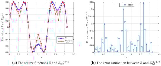
Figure 1. A comparison between $\mathsf{\Xi }$ and ${\mathsf{\Xi }}_{\alpha ,\tau }^{{\epsilon }_1,{\epsilon }_2,{\epsilon }_3}$ for $\beta =1.5$, $\mathbf{X}=\mathbf{T}=40$, $\{{\epsilon }_1,{\epsilon }_2,{\epsilon }_3\}$ := $\{9\times {10}^{-2},2\times {10}^{-2},1\times {10}^{-3}\}$, $\tau ={\displaystyle \frac{4}{5}}$.

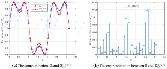
Figure 2. A comparison between $\mathsf{\Xi }$ and ${\mathsf{\Xi }}_{\alpha ,\tau }^{{\epsilon }_1,{\epsilon }_2,{\epsilon }_3}$ for $\beta =1.5$, $\mathbf{X}=\mathbf{T}=40$, $\{{\epsilon }_1,{\epsilon }_2,{\epsilon }_3\}$ := $\{1\times {10}^{-3},2\times {10}^{-3},3\times {10}^{-3}\}$, $\tau ={\displaystyle \frac{4}{5}}$.

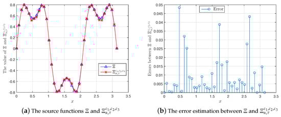
Figure 3. A comparison between $\mathsf{\Xi }$ and ${\mathsf{\Xi }}_{\alpha ,\tau }^{{\epsilon }_1,{\epsilon }_2,{\epsilon }_3}$ for $\beta =1.5$, $\mathbf{X}=\mathbf{T}=40$, $\{{\epsilon }_1,{\epsilon }_2,{\epsilon }_3\}$ := $\{3\times {10}^{-1},2\times {10}^{-2},5\times {10}^{-1}\}$, $\tau ={\displaystyle \frac{4}{5}}$.

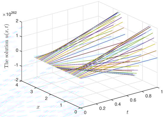
Figure 4. The solution $u(x,t)$ for $(x,t)\in (0,\pi )\times (0,1)$.

7. Conclusions

In this study, we use the Tikhonov method to regularize the inverse problem to determine an unknown source term in a space-time-fractional diffusion equation. By an example, we prove that this problem is ill-posed in the sense of Hadamard. Under a priori and a posteriori parameter choice rules, we show the results about the convergent estimate between the exact solution and the regularized solution. In addition, we show an example to illustrate our proposed regularization.

References

- Podlubny, I. Fractional Differential Equations. In Mathematics in Science and Engineering; Academic Press Inc.: San Diego, CA, USA, 1990; Volume 198. [Google Scholar]
- Nguyen, H.T.; Le, D.L.; Nguyen, T.V. Regularized solution of an inverse source problem for a time fractional diffusion equation. Appl. Math. Model. 2016, 40, 8244–8264. [Google Scholar] [CrossRef]
- Wei, T.; Wang, J. A modified quasi-boundary value method for an inverse source problem of the time-fractional diffusion equation. Appl. Numer. Math. 2014, 78, 95–111. [Google Scholar] [CrossRef]
- Wang, J.G.; Zhou, Y.B.; Wei, T. Two regularization methods to identify a space-dependent source for the time-fractional diffusion equation. Appl. Numer. Math. 2013, 68, 39–57. [Google Scholar] [CrossRef]
- Zhang, Z.Q.; Wei, T. Identifying an unknown source in time-fractional diffusion equation by a truncation method. Appl. Math. Comput. 2013, 219, 5972–5983. [Google Scholar] [CrossRef]
- Yang, F.; Liu, X.; Li, X.X. Landweber iterative regularization method for identifying the unknown source of the modified Helmholtz equation. Bound. Value Probl. 2017, 91. [Google Scholar] [CrossRef]
- Tatar, S.; Ulusoy, S. An inverse source problem for a one-dimensional space-time fractional diffusion equation. Appl. Anal. 2015, 94, 2233–2244. [Google Scholar] [CrossRef]
- Tatar, S.; Tinaztepe, R.; Ulusoy, S. Determination of an unknown source term in a space-time fractional diffusion equation. J. Frac. Calc. Appl. 2015, 6, 83–90. [Google Scholar]
- Tatar, S.; Tinaztepe, R.; Ulusoy, S. Simultaneous inversion for the exponents of the fractional time and space derivatives in the space-time fractional diffusion equation. Appl. Anal. 2016, 95, 1–23. [Google Scholar] [CrossRef]
- Tuan, N.H.; Long, L.D. Fourier truncation method for an inverse source problem for space-time fractional diffusion equation. Electron. J. Differ. Equ. 2017, 2017, 1–16. [Google Scholar]
- Mehrdad, L.; Dehghan, M. The use of Chebyshev cardinal functions for the solution of a partial differential equation with an unknown time-dependent coefficient subject to an extra measurement. J. Comput. Appl. Math. 2010, 235, 669–678. [Google Scholar]
- Pollard, H. The completely monotonic character of the Mittag-Leffler function Eα(-x). Bull. Am. Math. Soc. 1948, 54, 1115–1116. [Google Scholar] [CrossRef]
- Yang, M.; Liu, J.J. Solving a final value fractional diffusion problem by boundary condition regularization. Appl. Numer. Math. 2013, 66, 45–58. [Google Scholar] [CrossRef]
- Kilbas, A.A.; Srivastava, H.M.; Trujillo, J.J. Theory and Applications of Fractional Differential Equations; Elsevier Science Limited: Amsterdam, The Netherlands, 2006. [Google Scholar]
- Luchko, Y. Initial-boundary-value problems for the one-dimensional time-fractional diffusion equation. Fract. Calc. Appl. Anal. 2012, 15, 141–160. [Google Scholar] [CrossRef]
- Quan, Z.; Feng, X.L. A fractional Tikhonov method for solving a Cauchy problem of Helmholtz equation. Appl. Anal. 2017, 96, 1656–1668. [Google Scholar] [CrossRef]
- Trifce, S.; Tomovski, Z. The general time fractional wave equation for a vibrating string. J. Phys. A Math. Theor. 2010, 43, 055204. [Google Scholar]
- Trifce, S.; Ralf, M.; Zivorad, T. Fractional diffusion equation with a generalized Riemann–Liouville time fractional derivative. J. Phys. A Math. Theor. 2011, 44, 255203. [Google Scholar]
- Hilfer, R.; Seybold, H.J. Computation of the generalized Mittag-Leffler function and its inverse in the complex plane. Integral Transform Spec. Funct. 2006, 17, 37–652. [Google Scholar] [CrossRef]
- Seybold, H.; Hilfer, R. Numerical Algorithm for Calculating the Generalized Mittag-Leffler Function. SIAM J. Numer. Anal. 2008, 47, 69–88. [Google Scholar] [CrossRef]
- Kilbas, A.A.; Srivastava, H.M.; Trujillo, J.J. Theory and Application of Fractional differential equations. In North—Holland Mathematics Studies; Elsevier Science B.V.: Amsterdam, The Netherlands, 2006; Volume 204. [Google Scholar]
- Sakamoto, K.; Yamamoto, M. Initial value/boundary value problems for fractional diffusion-wave equations and applications to some inverse problems. J. Math. Anal. Appl. 2011, 382, 426–447. [Google Scholar] [CrossRef]
- Kirsch, A. An Introduction to the Mathematical Theory of Inverse Problem; Springer: Berlin, Germany, 1996. [Google Scholar]
© 2019 by the authors. Licensee MDPI, Basel, Switzerland. This article is an open access article distributed under the terms and conditions of the Creative Commons Attribution (CC BY) license (http://creativecommons.org/licenses/by/4.0/).