Model Formulation Over Lie Groups and Numerical Methods to Simulate the Motion of Gyrostats and Quadrotors

Abstract

The present paper recalls a formulation of non-conservative system dynamics through the Lagrange–d’Alembert principle expressed through a generalized Euler–Poincaré form of the system equation on a Lie group. The paper illustrates applications of the generalized Euler–Poincaré equations on the rotation groups to a gyrostat satellite and a quadcopter drone. The numerical solution of the dynamical equations on the rotation groups is tackled via a generalized forward Euler method and an explicit Runge–Kutta integration method tailored to Lie groups.

1. Introduction

The dynamics of non-conservative systems may be formulated through the Lagrange–d’Alembert principle. This very general principle allows one to deduce the general properties and laws of motion of bodies as well as of non-compressible, compressible and elastic liquids [1]. For continuous systems, the Lagrange–d’Alembert principle is formulated as a variational integral problem, which may be converted into a differential form known as the Euler–Poincaré equation. When the physical problem under investigation is subjected to smooth holonomic constraints, such as in the rigid-body case, the domain of the Euler–Poincaré equation becomes a smooth manifold and, under specific symmetries (i.e., the Lagrangian of the system is left-invariant), even a Lie group. In fact, Lie groups are special instances of differentiable manifolds that also carry on the structure of algebraic groups. In this event, one gets a reduced Euler–Poincaré equation on a Lie algebra paired to a companion differential equation on the associated Lie group. The resulting system of differential equations that describes completely the time-evolution of the system may be regarded as an initial-value problem on a tangent bundle. Such an initial value problem needs to be solved numerically on a computer platform by way of numerical methods that are specifically tailored to upholding the structure of the phase space.

The present paper of archival nature aims at presenting in details, and in a self-contained manner, two interlaced topics, namely:

1) Formulation of Euler–Poincaré equations of motion on Lie groups: This part, covered by Section 2 and Section 3, aims at recalling with some mathematical depth the Lagrange–d’Alembert principle expressed through a generalized Euler–Poincaré form. Moreover, this part aims at presenting in a detailed way the derivation of the reduced Lagrangian function for two systems, namely a satellite gyrostat and a quadrotor drone. In addition, this part aims at showing how the general Lagrange–d’Alembert principle boils down to equations of motion through their reduced Euler–Poincaré equations on the special orthogonal group $\mathrm{SO}\left(3\right)$.

2) Numerical integration of the Euler–Poincaré equations of motion: this part, covered by the Section 4 and Section 5, discusses the numerical solution of initial-value problems on smooth manifolds as an extension of two well-known techniques to numerically tackle classical initial-value problems, namely a forward Euler method and an explicit fourth-order Runge–Kutta method.

Section 6 presents some final remarks and concludes the paper.

2. The Lagrange–d’Alembert Principle and the Forced Euler–Poincaré Equation

We consider a non-conservative dynamical system whose state space is a Lie group $\mathbb{G}$. It is instrumental to recall the following definitions and properties [2,3] (see also [4,5]):

Lie group: a smooth manifold $\mathbb{G}$ that is also an algebraic group is termed a Lie group. An algebraic group is a structure $(\mathbb{G},m,i,e)$ where $m:\mathbb{G}\times \mathbb{G}\to \mathbb{G}$ is an associative binary operation termed group multiplication, $e\in \mathbb{G}$ is an identity element with respect to the multiplication, namely $m(g,e)=m(e,g)=g$ for any $g\in \mathbb{G}$, and $i:\mathbb{G}\to \mathbb{G}$ denotes inversion with respect to multiplication, namely $m\left(i\right(g),g)=m(g,i(g\left)\right)=e$ for any $g\in \mathbb{G}$. A left translation $L:\mathbb{G}\times \mathbb{G}\to \mathbb{G}$ is defined as $L_g\left(h\right):=m(i\left(g\right),h)$. (Our definition is not standard, we adopt it because it simplifies the notation and makes it apparent that left translation and group multiplication are different notions.) In this report, we deal with matrix Lie groups, therefore we may take $m(g,h):=gh$ (matrix multiplication), $i\left(g\right):=g^{-1}$ (matrix inversion) and the identity matrix as identity element. In this setting, $L_g\left(h\right)=g^{-1}h$.

Tangent bundle and metrization: given a state $g\in \mathbb{G}$, the tangent space to $\mathbb{G}$ at g will be denoted as $T_g\mathbb{G}$. The tangent bundle associated with a Lie group $\mathbb{G}$ is denoted by $T\mathbb{G}$ and plays the role of phase-space for a dynamical system whose state-space is $\mathbb{G}$. The inner product of two tangent vectors $\xi ,\eta \in T_g\mathbb{G}$ is denoted by ${⟨\xi ,\eta ⟩}_g$. A smooth function $F:\mathbb{G}\to \mathbb{G}$ induces a linear map $\mathrm{d}{F}_g:T_g\mathbb{G}\to T_{F\left(g\right)}\mathbb{G}$ termed pushforward. For a matrix Lie group, the pushforward map $\mathrm{d}{\left(L_g\right)}_h:T_h\mathbb{G}\to T_{g^{-1}h}\mathbb{G}$ associated to a left translation is $\mathrm{d}{\left(L_g\right)}_h\left(\eta \right):=g^{-1}\eta$.

Lie algebra: the tangent space $\mathfrak{g}:=T_e\mathbb{G}$ to a Lie group at the identity is termed Lie algebra. The Lie algebra is endowed with Lie brackets, denoted as $[·,·]:\mathfrak{g}\times \mathfrak{g}\to \mathfrak{g}$, and an adjoint endomorphism ${\mathrm{ad}}_{\xi }\eta :=[\xi ,\eta ]$. On a matrix Lie algebra, $[\xi ,\eta ]:=\xi \eta -\eta \xi$. A pushforward map $\mathrm{d}{\left(L_g\right)}_g:T_g\mathbb{G}\to \mathfrak{g}$ is denoted as $\mathrm{d}{L}_g$ for brevity. Given a smooth function $\ell :\mathfrak{g}\to \mathbb{R}$, for a matrix Lie group one may define the fiber derivative of ℓ, $\frac{\partial \ell }{\partial \xi }\in \mathfrak{g}$, at $\xi \in \mathfrak{g}$ as the unique algebra element such that ${⟨\frac{\partial \ell }{\partial \xi },\eta ⟩}_e=\mathrm{tr}\left({\left({\mathrm{J}}_{\xi }\ell \right)}^{\top }\eta \right)$ for any $\eta \in \mathfrak{g}$, where ${\mathrm{J}}_{\xi }\ell$ denotes the Jacobian matrix of the function ℓ with respect to the matrix $\xi$.

2.1. The Lagrange–d’Alembert Principle

The Lagrange–d’Alembert principle is one of the fundamental principles in mathematical physics to formulate the motion of a physical system on a differentiable manifold and to handle non-conservative forces. Let $\mathsf{\Lambda }:T\mathbb{G}\to \mathbb{R}$ denote a Lagrangian function and $F:T\mathbb{G}\to T\mathbb{G}$ a generalized force field (more precisely, a generalized force field is a smooth map from $T\mathbb{G}$ to its dual $T^{★}\mathbb{G}$ or, for left-invariant force fields, from an algebra $\mathfrak{g}$ to its dual ${\mathfrak{g}}^{★}$; again, we adopt this non-standard definition because it eases the notation). The Lagrange–d’Alembert principle affirms that a dynamical system generates a trajectory g such that:

$$\delta {\int }_a^b\mathsf{\Lambda }(g,\dot{g})\mathrm{d}t+{\int }_a^b{⟨F(g,\dot{g}),\delta g⟩}_g\mathrm{d}t=0,$$

(1)

where the symbol $\delta$ denotes variation, which vanish at endpoints and is elsewhere arbitrary and an over-dot (as in $\dot{g}$) denotes (partial) derivative with respect to the parameter t.

We recall that a variational principle consists in taking a continuous family of curves $g:U\subset {\mathbb{R}}^2\to \mathbb{G}$, denoted as $g(t,\epsilon )$, where the index $\epsilon$ selects a curve in the family and the index t denotes a point over this curve. All the curves in the family depart from the same initial point and arrive at the same endpoint, namely, $g(a,\epsilon )$ and $g(b,\epsilon )$ are constant with respect to $\epsilon$. The variations in Equation (1) are defined as

$$\begin{array}{c}\delta {\int }_a^b\mathsf{\Lambda }(g,\dot{g})\mathrm{d}t:={\left.{\int }_a^b\frac{\partial }{\partial \epsilon }\mathsf{\Lambda }(g(t,\epsilon ),\dot{g}(t,\epsilon ))\mathrm{d}t\right|}_{\epsilon =0},\end{array}$$

(2)

$$\delta g:={\left.\frac{\partial g(t,\epsilon )}{\partial \epsilon }\right|}_{\epsilon =0}.$$

(3)

The following lemma affords handling variational principles on Lie groups:

Lemma 1

([6]). Given a smooth function $g:U\subset {\mathbb{R}}^2\to \mathbb{G}$ on a matrix Lie group, define:

$$\begin{array}{c}\hfill \xi (t,\epsilon ):=\mathrm{d}{L}_{g(t,\epsilon )}\left(\frac{\partial g(t,\epsilon )}{\partial t}\right),\eta (t,\epsilon ):=\mathrm{d}{L}_{g(t,\epsilon )}\left(\frac{\partial g(t,\epsilon )}{\partial \epsilon }\right),\end{array}$$

(4)

where L denotes a left translation and $\mathrm{d}L$ its pushforward. Then, it holds that

$$\frac{\partial \xi }{\partial \epsilon }=\dot{\eta }+{\mathrm{ad}}_{\xi }\eta .$$

(5)

Proof. 

By definition, $\xi =g^{-1}\frac{\partial g}{\partial t}$ and $\eta =g^{-1}\frac{\partial g}{\partial \epsilon }$, therefore

$$\begin{array}{c}\frac{\partial \xi }{\partial \epsilon }=\frac{\partial g^{-1}}{\partial \epsilon }\frac{\partial g}{\partial t}+g^{-1}\frac{{\partial }^{2}g}{\partial \epsilon \partial t}=-g^{-1}\frac{\partial g}{\partial \epsilon }{g}^{-1}\frac{\partial g}{\partial t}+g^{-1}\frac{{\partial }^{2}g}{\partial \epsilon \partial t}=-\eta \xi +g^{-1}\frac{{\partial }^{2}g}{\partial \epsilon \partial t},\\ \frac{\partial \eta }{\partial t}=\frac{\partial g^{-1}}{\partial t}\frac{\partial g}{\partial \epsilon }+g^{-1}\frac{{\partial }^{2}g}{\partial t\partial \epsilon }=-g^{-1}\frac{\partial g}{\partial t}{g}^{-1}\frac{\partial g}{\partial \epsilon }+g^{-1}\frac{{\partial }^{2}g}{\partial t\partial \epsilon }=-\xi \eta +g^{-1}\frac{{\partial }^{2}g}{\partial t\partial \epsilon }.\end{array}$$

It follows that

$$\frac{\partial \xi }{\partial \epsilon }-\frac{\partial \eta }{\partial t}=\xi \eta -\eta \xi ={\mathrm{ad}}_{\xi }\eta ,$$

(6)

as in the text of the lemma. □

Assuming that the Lagrangian as well as the generalized force field F are left invariant, we may write $\mathsf{\Lambda }(g,\dot{g})=\ell \left(\mathrm{d}{L}_g\left(\dot{g}\right)\right)$ and $\mathrm{d}{L}_g\left(F(g,\dot{g})\right)=f\left(\mathrm{d}{L}_g\left(\dot{g}\right)\right)$, where $\ell :\mathfrak{g}\to \mathbb{R}$ and $f:\mathfrak{g}\to \mathfrak{g}$ denote a reduced Lagrangian and a reduced force field, respectively. In addition, if the inner product is left-invariant, it holds that

$${⟨F(g,\dot{g}),\delta g⟩}_g={⟨f\left(\mathrm{d}{L}_g\left(\dot{g}\right)\right),\mathrm{d}{L}_g\left(\delta g\right)⟩}_e.$$

(7)

Therefore, the integral Lagrange–d’Alembert principle (1) reduces to

$$\delta {\int }_a^b\ell \left(\mathrm{d}{L}_g\left(\dot{g}\right)\right)\mathrm{d}t+{\int }_a^b{⟨f\left(\mathrm{d}{L}_g\left(\dot{g}\right)\right),\mathrm{d}{L}_g\left(\delta g\right)⟩}_e\mathrm{d}t=0,$$

(8)

where it is legitimate to replace $\mathrm{d}{L}_g\left(\dot{g}\right)$ with $\xi$ and $\mathrm{d}{L}_g\left(\delta g\right)$ with $\eta$ and then set $\epsilon$ to 0.

2.2. The Forced Euler–Poincaré Equation

By means of the Lemma 1, the variations in the reduced Lagrange–d’Alembert principle may be worked out to derive equations of motion in differential form, as shown in the following.

Theorem 1 

([6]). Let $\xi :=\mathrm{d}{L}_g\left(\dot{g}\right)$ and $\eta :=\mathrm{d}{L}_g\left(\delta g\right)$. The solution of the integral Lagrange–d’Alembert Equation (8) under perturbations of the form $\frac{\partial \xi }{\partial \epsilon }=\dot{\eta }+{\mathrm{ad}}_{\xi }\eta$, which vanishes at endpoints, satisfies the Euler–Poincaré equation

$$\frac{\mathrm{d}}{\mathrm{d}t}\frac{\partial \ell }{\partial \xi }={\mathrm{ad}}_{\xi }^{★}\left(\frac{\partial \ell }{\partial \xi }\right)+f.$$

(9)

Proof. 

For the first term in (8), it holds that

$$\frac{\partial }{\partial \epsilon }\ell \left(\mathrm{d}{L}_g\left(\frac{\partial g}{\partial t}\right)\right)={⟨\frac{\partial \ell }{\partial \xi },\frac{\partial \xi }{\partial \epsilon }⟩}_e,$$

(10)

where $\frac{\partial \ell }{\partial \xi }\in \mathfrak{g}$ denotes the fiber derivative of the reduced Lagrangian and $\xi :=\mathrm{d}{L}_g\left(\dot{g}\right)$. For the second term in (8), it holds that

$${⟨f\left(\mathrm{d}{L}_g\left(\dot{g}\right)\right),\mathrm{d}{L}_g\left(\frac{\partial g}{\partial \epsilon }\right)⟩}_e={⟨f,\eta ⟩}_e,$$

(11)

where $\eta :=\mathrm{d}{L}_g\left(\frac{\partial g}{\partial \epsilon }\right)$. Recall that both fields $\xi$ and $\eta$ depend on t as well as on $\epsilon$. The Equation (8), thanks to the equivalences (10) and (11) and to the relation (5), yields

$${\int }_a^b\left({⟨\frac{\partial \ell }{\partial \xi },\dot{\eta }+{\mathrm{ad}}_{\xi }\eta ⟩}_e+{⟨f,\eta ⟩}_e\right)\mathrm{d}t=0.$$

(12)

Integration by parts yields

$${\int }_a^b{⟨\frac{\partial \ell }{\partial \xi },\dot{\eta }⟩}_e\mathrm{d}t={\int }_a^b{⟨-\frac{\mathrm{d}}{\mathrm{d}t}\frac{\partial \ell }{\partial \xi },\eta ⟩}_e\mathrm{d}t$$

(13)

because the perturbation $\eta$ vanishes at the endpoints, therefore the Equation (12) becomes

$${\int }_a^b\left({⟨\frac{\partial \ell }{\partial \xi },{\mathrm{ad}}_{\xi }\eta ⟩}_e+{⟨-\frac{\mathrm{d}}{\mathrm{d}t}\frac{\partial \ell }{\partial \xi }+f,\eta ⟩}_e\right)\mathrm{d}t=0$$

(14)

or, equivalently, introducing the conjugate ${\mathrm{ad}}_{\xi }^{★}$ of the adjoint operator with respect to the metric,

$${\int }_a^b{⟨-\frac{\mathrm{d}}{\mathrm{d}t}\frac{\partial \ell }{\partial \xi }+f+{\mathrm{ad}}_{\xi }^{★}\left(\frac{\partial \ell }{\partial \xi }\right),\eta ⟩}_e\mathrm{d}t=0.$$

(15)

Setting $\epsilon =0$ and recalling that the perturbation $\eta$ is arbitrary in the above equality implies the assertion. □

The complete dynamical equations then reads

$$\left\{\begin{array}{c}\dot{g}={\left(\mathrm{d}{L}_g\right)}^{-1}\left(\xi \right),\hfill \\ \frac{\mathrm{d}}{\mathrm{d}t}\frac{\partial \ell }{\partial \xi }={\mathrm{ad}}_{\xi }^{★}\left(\frac{\partial \ell }{\partial \xi }\right)+f.\hfill \end{array}\right.$$

(16)

The forcing term takes into account a number of external driving phenomena, such as

Rayeigh dissipation: this phenomenon is a form of energy dissipation due, e.g., to friction. The forcing term due to Rayleigh dissipation is written as $f_{\mathrm{R}}=-\frac{\partial \rho }{\partial \xi }$, where $\rho :\mathfrak{g}\to \mathbb{R}$ is a Rayleigh function [6]. For instance, a quadratic function of the state variable $\xi$ leads to a linear dissipation term known as viscous (or aerodynamic) drag.

Other driving causes: other than dissipation, the structure of the forcing term is free and depends on the problem under investigation, as long as it provides a map onto $\mathfrak{g}$. This leaves room to incorporate into f control terms, for instance, to stabilize the motion or to drive a dynamical system as discussed, for instance, in [7].

There exist by now quite detailed books, papers, and reviews about these concepts, including the book by Marsden and Ratiu [8] and the two volumes by Holm [9,10], where these notions are explained in great details and with a number of examples going from the single rigid body to more complex multi-body dynamics problems.

3. Rigid-Body Equations

This section introduces two cases of study based on the Lie group $\mathbb{G}:=SO\left(3\right)$ of three-dimensional rotations. The group is defined as $SO\left(3\right):=\{R\in {\mathbb{R}}^{3\times 3}\mid R^{\top }R=R{R}^{\top }=I_3,det\left(R\right)=+1\}$ and its Lie algebra is $\mathfrak{so}\left(3\right):=\{\xi \in {\mathbb{R}}^{3\times 3}\mid \xi +{\xi }^{\top }=0\}$. The symbol ${}^{\top }$ denotes matrix transpose and the quantity $I_3$ represents a $3\times 3$ identity matrix.

Let us elaborate on the notion of dual adjoint operator on the Lie algebra $\mathfrak{so}\left(3\right)$.

Lemma 2.

Let the vector space$\mathfrak{so}\left(3\right)$be endowed with the canonical inner product$⟨\xi ,\eta ⟩:=-\mathrm{tr}\left(\xi \eta \right)$, and define the linear endomorphism${\mathrm{ad}}_{\xi }\left(\eta \right):=\xi \eta -\eta \xi$. The dual of the adjoint operator with respect to the canonical inner product is${\mathrm{ad}}_{\xi }^{★}=-{\mathrm{ad}}_{\xi }$.

Proof. 

Take three $\mathfrak{so}\left(3\right)$-vectors $\xi ,\eta ,\zeta$ and compute

$$⟨{\mathrm{ad}}_{\xi }\left(\eta \right),\zeta ⟩=-\mathrm{tr}\left(\right(\xi \eta -\eta \xi \left)\zeta \right)=\mathrm{tr}\left(\eta \right(\xi \zeta -\zeta \xi \left)\right),$$

(17)

$$⟨\eta ,{\mathrm{ad}}_{\xi }^{★}\left(\zeta \right)⟩=-\mathrm{tr}(\eta {\mathrm{ad}}_{\xi }^{★}\left(\zeta \right)).$$

(18)

By definition of dual operator with respect to a metric, it must hold that $⟨{\mathrm{ad}}_{\xi }\left(\eta \right),\zeta ⟩=⟨\eta ,{\mathrm{ad}}_{\xi }^{★}\left(\zeta \right)⟩$ for any $\eta$, therefore the assertion follows. □

Since, in the state space $\mathbb{G}:=SO\left(3\right)$, it holds that ${\left(\mathrm{d}{L}_R\right)}^{-1}\left(\xi \right)=R\xi$ and ${\mathrm{ad}}_{\xi }^{★}\eta =-{\mathrm{ad}}_{\xi }\eta$ (by Lemma 2), the Euler–Poincaré equations read

$$\left\{\begin{array}{c}\dot{R}=R\xi ,\hfill \\ \frac{\mathrm{d}}{\mathrm{d}t}\frac{\partial \ell }{\partial \xi }=-{\mathrm{ad}}_{\xi }\left(\frac{\partial \ell }{\partial \xi }\right)+\tau ,\hfill \end{array}\right.$$

(19)

where $\tau$ is an instance of generalized force and denotes the resultant of all external mechanical torques. In this context, the state variable $g:=R$ denotes the attitude of a rigid body and the state-variable $\xi$ denotes its instantaneous angular velocity.

It is convenient to define the operator $〚·〛$ as:

$$〚x〛:=\left[\begin{array}{ccc}0& -x_3& x_2\\ x_3& 0& -x_1\\ -x_2& x_1& 0\end{array}\right].$$

(20)

Since any skew-symmetric matrix in $\mathfrak{so}\left(3\right)$ may be written as in Equation (20), it is convenient to define a basis of this vector space as follows:

$$\mathfrak{so}\left(3\right)=\mathrm{span}({\xi }_x,{\xi }_y,{\xi }_z),with$$

(21)

$${\xi }_x:=\left[\begin{array}{ccc}0& 0& 0\\ 0& 0& -1\\ 0& 1& 0\end{array}\right],{\xi }_y:=\left[\begin{array}{ccc}0& 0& 1\\ 0& 0& 0\\ -1& 0& 0\end{array}\right],{\xi }_z:=\left[\begin{array}{ccc}0& -1& 0\\ 1& 0& 0\\ 0& 0& 0\end{array}\right].$$

(22)

In the present setting, we take the canonical metric ${⟨\xi ,\eta ⟩}_e:=\mathrm{tr}\left({\xi }^{\top }\eta \right)$. With this choice, it not difficult to show that

$$\frac{\partial \ell }{\partial \xi }=\frac{1}{2}({\mathrm{J}}_{\xi }\ell -{\mathrm{J}}_{\xi }^{\top }\ell ).$$

(23)

In order to shorten some relations, it is also convenient to introduce the matrix anti-commutator $\{A,B\}:=AB+BA$. The anti-commutator is a symmetric form, namely ${\{A,B\}}^{\top }=\{A,B\}$, and linear in both arguments. Conversely, the matrix commutator in $\mathfrak{so}\left(3\right)$ is an anti-symmetric bilinear form, namely $[\xi ,\eta ]+[\eta ,\xi ]=0$. (We skip the Jacobi identity that plays no role in this paper.)

Moreover, it is convenient to recall a property of the matrix ‘trace’ operator, namely $\mathrm{tr}\left(ABC\right)=\mathrm{tr}\left(BCA\right)=\mathrm{tr}\left(CAB\right)$ for any square $A,B,C$.

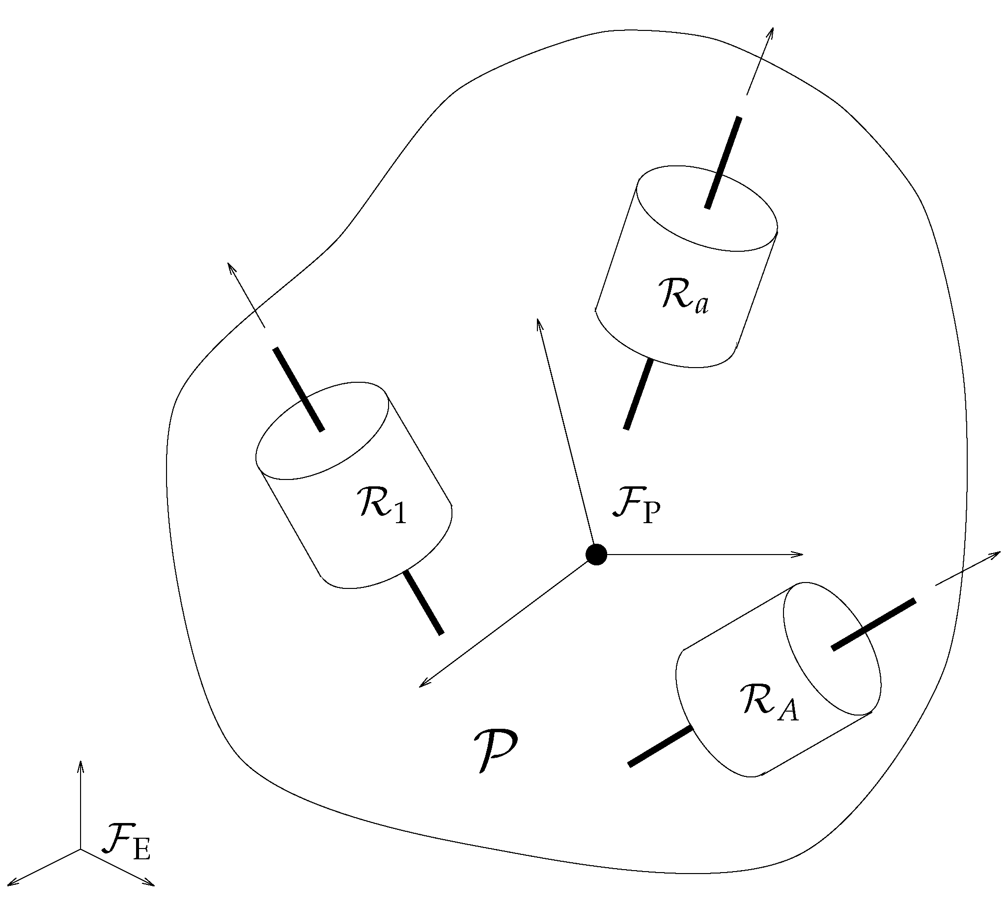
3.1. Satellite Gyrostat

The dynamics of rotating bodies is a classic topic in mechanics. Several aspects of the motion of a rotating rigid body were investigated in the eighteenth and nineteenth centuries, but the study of the dynamics of rotating bodies is still very important for numerous applications as in satellite gyrostat, spacecraft, and robotics [11]. The gyrostats are scientific models or instruments designed to illustrate experimentally the dynamics of a rotating body such as the spinning-top, the hoop and the bicycle, and also the precession of the equinox and the rotation of the earth. The original gyrostat is an instrument designed by Lord Kelvin to illustrate the complicated state of motion of a spinning body when free to wander about on a horizontal plane, like a top spun on the pavement, or a hoop or bicycle on the road [12]. It consists of a massive flywheel concealed in a metal casing. In general, a gyrostat is a system of bodies whose relative motion does not alter the intrinsic mass distribution of the system. A solid gyrostat is an arbitrary rigid body attached to one or more axisymmetric rotors with their axes fixed in the carrier [12].

Let us consider the case of a satellite represented by a gyrostat as in [7,13]. A satellite gyrostat is a suspended rigid body, termed platform, that contains one or more rigid wheels, termed rotors, that are spinning around fixed axes. Since the total angular momentum must stay constant, a rotation of the wheels causes a global counter-rotation of the gyrostat, which makes it possible to stabilize its motion (known as the principle of momentum transfer [13]).

In this paper, the interactions of the translational motion of a gyrostat satellite on its attitude dynamics is completely neglected. Assuming that the center of the gyrostat is fixed in space, one may attach an inertial reference frame ${\mathcal{F}}_{\mathrm{E}}$ to the center and denote by $x_0\in {\mathbb{R}}^3$ the position of each infinitesimal volume of the platform in a platform-fixed reference frame ${\mathcal{F}}_{\mathrm{P}}$, as shown in the Figure 1.

Figure 1. Gyrostat reference frames (adapted from [13]).

At any time t, the position of the infinitesimal volume with respect to ${\mathcal{F}}_{\mathrm{E}}$ is $x\in {\mathbb{R}}^3$ and, since the platform is a rigid body, $x\left(t\right)=R\left(t\right)x_0$, where $R\in SO\left(3\right)$ denotes a rotation matrix that takes the platform-fixed frame ${\mathcal{F}}_{\mathrm{P}}$ to coincide with ${\mathcal{F}}_{\mathrm{E}}$. The kinetic energy of the platform $\mathcal{P}$ with respect to the inertial reference frame ${\mathcal{F}}_{\mathrm{E}}$ may be written as

$$k_{\mathrm{p}}:=\frac{1}{2}\underset{\mathcal{P}}{\int }{\parallel \dot{x}\parallel }^2\mathrm{d}m,$$

(24)

where $\mathrm{d}m$ denotes the mass content of the infinitesimal volume. Recalling that $\parallel \dot{x}{\parallel }^2=\mathrm{tr}\left(\dot{x}{\dot{x}}^{\top }\right)$, $\dot{x}=\dot{R}{x}_0$, and that $\dot{R}=R\xi$, with $\xi \in \mathfrak{so}\left(3\right)$, we get:

$$k_{\mathrm{p}}=\frac{1}{2}\underset{\mathcal{P}}{\int }\mathrm{tr}\left(\dot{x}{\dot{x}}^{\top }\right)\mathrm{d}m=\frac{1}{2}\underset{\mathcal{P}}{\int }\mathrm{tr}\left(R\xi x_0{x}_0^{\top }{\xi }^{\top }{R}^{\top }\right)\mathrm{d}m=\frac{1}{2}\mathrm{tr}\left(\xi {\widehat{J}}_{\mathrm{p}}{\xi }^{\top }\right),$$

(25)

where $\mathrm{tr}(·)$ denotes matrix trace and ${\widehat{J}}_{\mathrm{p}}\in {\mathbb{R}}^{3\times 3}$ is defined as

$${\widehat{J}}_{\mathrm{p}}:=\underset{\mathcal{P}}{\int }{x}_0{x}_0^{\top }\mathrm{d}m$$

(26)

and denotes a non-standard inertia tensor [14]. The standard inertia tensor of the platform is defined as

$$J_{\mathrm{p}}:=\underset{\mathcal{P}}{\int }〚x_0〛〚x_0{〛}^{\top }\mathrm{d}m.$$

(27)

These inertia tensors are related as outlined in the following

Lemma 3

([14]). The non-standard moment of inertia $\widehat{J}$ of a body is related to its standard moment of inertia J by the relationship $\widehat{J}=\frac{1}{2}\mathrm{tr}\left(J\right)I_3-J$.

In addition, assume that the gyrostat contains A rotors spinning on fixed axis inside the platform. Each rotor is indexed by $a=1,2,\dots ,A$. The coordinate of the center of each rotor in the platform-fixed reference system ${\mathcal{F}}_{\mathrm{P}}$ is denoted as $c_a\in {\mathbb{R}}^3$ and the rotation matrix that describes the spinning of each rotor with respect to ${\mathcal{F}}_{\mathrm{P}}$ is denoted as $R_a\in \mathrm{SO}\left(3\right)$. For a specific rotor ${\mathcal{R}}_a$, the coordinate of each volume element in this rotor, with respect to the reference frame ${\mathcal{F}}_{\mathrm{P}}$, at time t is $x\left(t\right)=R\left(t\right)(c_a+R_a\left(t\right)s)$, where $s\in {\mathbb{R}}^3$ denotes the position of the volume element in a rotor-fixed reference system. Apparently, it holds that

$$\dot{x}=\dot{R}(c_a+R_{a}s)+R{\dot{R}}_{a}s\Rightarrow R^{\top }\dot{x}=\xi c_a+(\xi R_a+{\dot{R}}_a)s.$$

(28)

Consequently, the kinetic energy per mass element $\mathrm{d}m$ of the rotor ${\mathcal{R}}_a$ may be written as

$$\begin{array}{c}\frac{1}{2}\mathrm{tr}\left(\dot{x}{\dot{x}}^{\top }\right)=\frac{1}{2}\mathrm{tr}\left(\left(R^{\top }\dot{x}\right){\left(R^{\top }\dot{x}\right)}^{\top }\right)\hfill \\ =\frac{1}{2}\mathrm{tr}\left(\xi c_a{c}_a^{\top }{\xi }^{\top }\right)+\frac{1}{2}\mathrm{tr}\left((\xi R_a+{\dot{R}}_a)s{s}^{\top }{(\xi R_a+{\dot{R}}_a)}^{\top }\right)+\mathrm{tr}\left(\xi c_a{s}^{\top }{(\xi R_a+{\dot{R}}_a)}^{\top }\right).\end{array}$$

(29)

The kinetic energy of each spinning rotor ${\mathcal{R}}_a$ in the earth frame ${\mathcal{F}}_{\mathrm{E}}$ may be written as

$$k_a:=\frac{1}{2}\underset{{\mathcal{R}}_a}{\int }\mathrm{tr}\left(\left(R^{\top }\dot{x}\right){\left(R^{\top }\dot{x}\right)}^{\top }\right)\mathrm{d}m,$$

(30)

and straightforward calculations lead to the expression

$$k_a=\frac{1}{2}{M}_a\mathrm{tr}\left(\xi c_a{c}_a^{\top }{\xi }^{\top }\right)+\frac{1}{2}\mathrm{tr}\left((\xi R_a+{\dot{R}}_a){\widehat{J}}_a{(\xi R_a+{\dot{R}}_a)}^{\top }\right)+M_a\mathrm{tr}\left(\xi c_a{\overline{c}}_a^{\top }{(\xi R_a+{\dot{R}}_a)}^{\top }\right),$$

(31)

where

$$M_a:=\underset{{\mathcal{R}}_a}{\int }\mathrm{d}m,{\widehat{J}}_a:=\underset{{\mathcal{R}}_a}{\int }s{s}^{\top }\mathrm{d}m \mathrm{a}\mathrm{n}\mathrm{d} {\overline{c}}_a:=\frac{1}{M_a}\underset{{\mathcal{R}}_a}{\int }s\mathrm{d}m.$$

(32)

In order to simplify Equation (31), we assume that each rotor is symmetric about its center of mass, which implies that ${\overline{c}}_a=0$. Moreover, we assume that each rotor may be schematized as a cylinder spinning around its central axis, which implies that $R_a{\widehat{J}}_a{R}_a^{\top }={\widehat{J}}_a$. The following lemma studies a special case where this result holds true.

Lemma 4.

Take a cylindrical rotor spinning around the z axis, whose rotation matrix is denoted by$R_z\left(t\right)$and its non-standard inertia matrix is denoted by${\widehat{J}}_{\mathrm{cyl}}$. It holds that$R_z\left(t\right){\widehat{J}}_{\mathrm{cyl}}{R}_z^{\top }\left(t\right)={\widehat{J}}_{\mathrm{cyl}}$.

Proof. 

Because of symmetry, the inertia tensor of the cylindrical body and its orientation matrix take the form

$$J_{\mathrm{cyl}}=\left[\begin{array}{ccc}{J}_{xy}& 0& 0\\ 0& J_{xy}& 0\\ 0& 0& J_{zz}\end{array}\right],R_z\left(t\right)=\left[\begin{array}{ccc}cos\left({\theta }_z\left(t\right)\right)& -sin\left({\theta }_z\left(t\right)\right)& 0\\ sin\left({\theta }_z\left(t\right)\right)& cos\left({\theta }_z\left(t\right)\right)& 0\\ 0& 0& 1\end{array}\right].$$

(33)

Its non-standard inertia tensor ${\widehat{J}}_{\mathrm{cyl}}=\frac{1}{2}\mathrm{tr}\left(J_{\mathrm{cyl}}\right)I_3-J_{\mathrm{cyl}}$ is

$${\widehat{J}}_{\mathrm{cyl}}=\left[\begin{array}{ccc}\frac{J_{zz}}{2}& 0& 0\\ 0& \frac{J_{zz}}{2}& 0\\ 0& 0& J_{xy}-\frac{J_{zz}}{2}\end{array}\right],$$

(34)

therefore

$$R_z\left(t\right){\widehat{J}}_{\mathrm{cyl}}{R}_z^{\top }\left(t\right)=\left[\begin{array}{ccc}cos\left({\theta }_z\left(t\right)\right)& -sin\left({\theta }_z\left(t\right)\right)& 0\\ sin\left({\theta }_z\left(t\right)\right)& cos\left({\theta }_z\left(t\right)\right)& 0\\ 0& 0& 1\end{array}\right]\left[\begin{array}{ccc}\frac{J_{zz}}{2}& 0& 0\\ 0& \frac{J_{zz}}{2}& 0\\ 0& 0& J_{xy}-\frac{J_{zz}}{2}\end{array}\right]\left[\begin{array}{ccc}cos\left({\theta }_z\left(t\right)\right)& sin\left({\theta }_z\left(t\right)\right)& 0\\ -sin\left({\theta }_z\left(t\right)\right)& cos\left({\theta }_z\left(t\right)\right)& 0\\ 0& 0& 1\end{array}\right].$$

Computing the matrix products, it is not difficult to find that $R_z\left(t\right){\widehat{J}}_{\mathrm{cyl}}{R}_z^{\top }\left(t\right)={\widehat{J}}_{\mathrm{cyl}}$, irrespective of ${\theta }_z\left(t\right)$. □

Recalling that ${\dot{R}}_a={\xi }_a{R}_a$, the expression (31) becomes

$$\begin{array}{c}{k}_a=\frac{1}{2}{M}_a\mathrm{tr}\left(\xi c_a{c}_a^{\top }{\xi }^{\top }\right)+\frac{1}{2}\mathrm{tr}\left((\xi +{\xi }_a)R_a{\widehat{J}}_a{R}_a^{\top }{(\xi +{\xi }_a)}^{\top }\right)\hfill \\ =\frac{1}{2}{M}_a\mathrm{tr}\left(\xi c_a{c}_a^{\top }{\xi }^{\top }\right)+\frac{1}{2}\mathrm{tr}\left((\xi +{\xi }_a){\widehat{J}}_a{(\xi +{\xi }_a)}^{\top }\right).\hfill \end{array}$$

(35)

The angular momentum ${\xi }_a$ is a datum because the spinning of a rotor is an externally-controlled variable.

The total kinetic energy of the gyrostat is hence given by

$$\begin{array}{c}k:=k_{\mathrm{p}}+\sum _{a=1}^A{k}_a\hfill \\ =\frac{1}{2}\mathrm{tr}\left(\xi {\widehat{J}}_{\mathrm{p}}{\xi }^{\top }\right)+\frac{1}{2}\sum _{a=1}^A{M}_a\mathrm{tr}\left(\xi c_a{c}_a^{\top }{\xi }^{\top }\right)+\frac{1}{2}\sum _{a=1}^A\mathrm{tr}\left((\xi +{\xi }_a){\widehat{J}}_a{(\xi +{\xi }_a)}^{\top }\right)\hfill \\ =\frac{1}{2}\mathrm{tr}\left(\xi \widehat{J}{\xi }^{\top }\right)+\frac{1}{2}\sum _{a=1}^A\mathrm{tr}\left((\xi +{\xi }_a){\widehat{J}}_a{(\xi +{\xi }_a)}^{\top }\right),\hfill \end{array}$$

(36)

where $\widehat{J}:={\widehat{J}}_{\mathrm{p}}+{\sum }_{a=1}^A{M}_a{c}_a{c}_a^{\top }$. The spinning of the rotors is assumed to be frictionless. Notice that, upon defining $C:=[c_1{c}_2\cdots c_A]$, the non-standard inertia tensor may be rewritten as $\widehat{J}={\widehat{J}}_{\mathrm{p}}+C\mathrm{diag}(M_1,M_2,\dots ,M_A)C^{\top }$ [13].

In the following, we write explicitly the equations of motion of a gyrostat in a number of cases. In all cases, the system is supposed to be subjected to a constant potential energy, which may be assumed to be 0 without loss of generality. The potential energy is non-constant in the case that the gyrostat is subjected, e.g., to a gravitational field, as explained in [15].

3.1.1. Frictionless Gyrostat with Blocked Rotors

This case corresponds to non-spinning rotors. Analytically, this condition corresponds to the case that all ${\xi }_a=0$. In addition, no friction is assumed for the rotation of the gyrostat. The reduced Lagrangian of the gyrostat hence reads

$$\ell \left(\xi \right):=\frac{1}{2}\mathrm{tr}\left(\xi \widehat{J}{\xi }^{\top }\right)+\frac{1}{2}\sum _{a=1}^A\mathrm{tr}\left(\xi {\widehat{J}}_a{\xi }^{\top }\right)=\frac{1}{2}\mathrm{tr}\left(\xi {\widehat{J}}_{\mathrm{g}}{\xi }^{\top }\right),$$

(37)

where ${\widehat{J}}_{\mathrm{g}}:=\widehat{J}+{\sum }_{a=1}^A{\widehat{J}}_a$ denotes the total tensor of inertia of the gyrostat (platform plus non-spinning rotors).

In order to write explicitly the Euler–Poincaré Equation (19), it is necessary to compute the fiber derivative of the reduced Lagrangian:

$$\frac{\partial \ell }{\partial \xi }=\frac{1}{2}({\widehat{J}}_{\mathrm{g}}\xi +\xi {\widehat{J}}_{\mathrm{g}})=\frac{1}{2}\{{\widehat{J}}_{\mathrm{g}},\xi \}.$$

(38)

Recalling that $-{\mathrm{ad}}_{\xi }\eta =\eta \xi -\xi \eta$, the Euler-Poicaré equation reads $\{{\widehat{J}}_{\mathrm{g}},\dot{\xi }\}=[\{{\widehat{J}}_{\mathrm{g}},\xi \},\xi ]$. Observing that $[\{{\widehat{J}}_{\mathrm{g}},\xi \},\xi ]=[{\widehat{J}}_{\mathrm{g}},{\xi }^2]$, the equations of motion may be written as

$$\left\{\begin{array}{c}\dot{R}=R\xi ,\hfill \\ \{{\widehat{J}}_{\mathrm{g}},\dot{\xi }\}=[{\widehat{J}}_{\mathrm{g}},{\xi }^2].\hfill \end{array}\right.$$

(39)

It is not difficult to recognize that the second equation is the classical Euler equation of rotation of an asymmetric rigid body under its own angular momentum unbalance. In fact, taking the platform-fixed reference system ${\mathcal{F}}_{\mathrm{P}}$ coincident with the principal axes of inertia and writing

$$J_{\mathrm{g}}=\left[\begin{array}{ccc}{J}_x& 0& 0\\ 0& J_y& 0\\ 0& 0& J_z\end{array}\right],\xi =\left[\begin{array}{ccc}0& -{\omega }_z& {\omega }_y\\ {\omega }_z& 0& -{\omega }_x\\ -{\omega }_y& {\omega }_x& 0\end{array}\right],$$

(40)

it is easy to see that the non-standard tensor of inertia for this configuration is

$${\widehat{J}}_{\mathrm{g}}=\frac{1}{2}\mathrm{tr}\left(J_{\mathrm{g}}\right)I_3-J_{\mathrm{g}}=\frac{1}{2}\left[\begin{array}{ccc}{J}_y-J_x+J_z& 0& 0\\ 0& J_x-J_y+J_z& 0\\ 0& 0& J_x+J_y-J_z\end{array}\right].$$

(41)

Therefore, by matrix calculations:

$$\{{\widehat{J}}_{\mathrm{g}},\dot{\xi }\}={\widehat{J}}_{\mathrm{g}}\dot{\xi }+\dot{\xi }{\widehat{J}}_{\mathrm{g}}=\left[\begin{array}{ccc}0& -J_z{\dot{\omega }}_z& J_y{\dot{\omega }}_y\\ J_z{\dot{\omega }}_z& 0& -J_x{\dot{\omega }}_x\\ -J_y{\dot{\omega }}_y& J_x{\dot{\omega }}_x& 0\end{array}\right],$$

(42)

$$[{\widehat{J}}_{\mathrm{g}},{\xi }^2]=\left[\begin{array}{ccc}0& -{\omega }_x{\omega }_y(J_x-J_y)& -{\omega }_x{\omega }_z(J_x-J_z)\\ {\omega }_x{\omega }_y(J_x-J_y)& 0& -{\omega }_y{\omega }_z(J_y-J_z)\\ {\omega }_x{\omega }_z(J_x-J_z)& {\omega }_y{\omega }_z(J_y-J_z)& 0\end{array}\right].$$

(43)

By equating the homologous entries of the above matrices one gets the classical Euler equations:

$${\dot{\omega }}_x=\frac{J_y-J_z}{J_x}{\omega }_y{\omega }_z,$$

(44)

$${\dot{\omega }}_y=\frac{J_z-J_x}{J_y}{\omega }_x{\omega }_z,$$

(45)

$${\dot{\omega }}_z=\frac{J_x-J_y}{J_z}{\omega }_x{\omega }_y.$$

(46)

Notice that for a ‘needle’ gyrostat (say, $J_z=0$), the Euler equations degenerate. Furthermore, if the inertia tensor is spherical, namely $J_x=J_y=J_z$, then the platform spins at constant angular speed around a non-precessing axis.

Besides, by using the notation introduced in this subsection, it is not difficult to show that

$$\frac{\partial \ell }{\partial \xi }=\frac{\partial \ell }{\partial {\omega }_x}{\xi }_x+\frac{\partial \ell }{\partial {\omega }_y}{\xi }_y+\frac{\partial \ell }{\partial {\omega }_z}{\xi }_z.$$

(47)

3.1.2. Frictionless Gyrostat with Spinning Rotors

We consider now the case of $A=3$ rotors positioned along the three axes of inertia of the gyrostat as studied in [7]. This configuration noticeably simplifies the equations and makes it easy to simulate the motion dynamics of the satellite, as well as to design proper control strategies. The rotors along the x ($a=1$) and the y ($a=2$) axes spin with constant angular velocity, while the rotor along the z axis ($a=3$) spins with oscillating angular velocity, namely:

$${\xi }_1=\left[\begin{array}{ccc}0& 0& 0\\ 0& 0& -{\omega }_1\\ 0& {\omega }_1& 0\end{array}\right],\mathrm{with}\mathrm{standard}\mathrm{inertia}\mathrm{tensor}{J}_1=\left[\begin{array}{ccc}{J}_{11}& 0& 0\\ 0& ★& 0\\ 0& 0& ★\end{array}\right],$$

(48)

$${\xi }_2=\left[\begin{array}{ccc}0& 0& {\omega }_2\\ 0& 0& 0\\ -{\omega }_2& 0& 0\end{array}\right],\mathrm{with}\mathrm{standard}\mathrm{inertia}\mathrm{tensor}{J}_2=\left[\begin{array}{ccc}★& 0& 0\\ 0& J_{22}& 0\\ 0& 0& ★\end{array}\right],$$

(49)

$${\xi }_3=\left[\begin{array}{ccc}0& -{\omega }_3(1+bcos\left(\nu t\right))& 0\\ {\omega }_3(1+bcos\left(\nu t\right))& 0& 0\\ 0& 0& 0\end{array}\right],\mathrm{with}{J}_3=\left[\begin{array}{ccc}★& 0& 0\\ 0& ★& 0\\ 0& 0& J_{33}\end{array}\right],$$

(50)

where ${\omega }_1,{\omega }_2,{\omega }_3>0$, $J_{11},J_{22},J_{33}>0$, $b>0$ and $\nu >0$ are given constants and the symbol ☆ denotes two identical unessential parameters per inertia tensor.

The reduced time-dependent Lagrangian reads

$$\ell (t,\xi ):=\frac{1}{2}\mathrm{tr}\left(\xi \widehat{J}{\xi }^{\top }\right)+\frac{1}{2}\sum _{a=1}^3\mathrm{tr}\left((\xi +{\xi }_a){\widehat{J}}_a{(\xi +{\xi }_a)}^{\top }\right)$$

(51)

and its fiber derivatives takes the form

$$\frac{\partial \ell }{\partial \xi }=\frac{1}{2}\{\widehat{J},\xi \}+\frac{1}{2}\sum _{a=1}^3\{{\widehat{J}}_a,\xi +{\xi }_a\}=\frac{1}{2}\{{\widehat{J}}_{\mathrm{g}},\xi \}+\frac{1}{2}\sum _{a=1}^3\{{\widehat{J}}_a,{\xi }_a\},$$

(52)

where ${\widehat{J}}_{\mathrm{g}}:=\widehat{J}+{\sum }_{a=1}^3{\widehat{J}}_a$. Since everything is constant with respect to the time t except for $\xi$ and ${\xi }_3$, it holds that

$$\frac{\mathrm{d}}{\mathrm{d}t}\frac{\partial \ell }{\partial \xi }=\frac{1}{2}\{{\widehat{J}}_{\mathrm{g}},\dot{\xi }\}+\frac{1}{2}{J}_{33}{\dot{\xi }}_3,$$

(53)

with

$${\dot{\xi }}_3=\left[\begin{array}{ccc}0& {\omega }_{3}b\nu sin\left(\nu t\right)& 0\\ -{\omega }_{3}b\nu sin\left(\nu t\right)& 0& 0\\ 0& 0& 0\end{array}\right].$$

(54)

Let us take again

$$J_{\mathrm{g}}=\left[\begin{array}{ccc}{J}_x& 0& 0\\ 0& J_y& 0\\ 0& 0& J_z\end{array}\right],\xi =\left[\begin{array}{ccc}0& -{\omega }_z& {\omega }_y\\ {\omega }_z& 0& -{\omega }_x\\ -{\omega }_y& {\omega }_x& 0\end{array}\right],$$

and the non-standard inertia tensor of the gyrostat is as in (41). For a frictionless gyrostat with spinning rotors, the Euler-Poicaré equation reads

$$\frac{1}{2}\{{\widehat{J}}_{\mathrm{g}},\dot{\xi }\}+\frac{1}{2}{J}_{33}{\dot{\xi }}_3=\left[\frac{1}{2}\{{\widehat{J}}_{\mathrm{g}},\xi \}+\frac{1}{2}{J}_{11}{\xi }_1+\frac{1}{2}{J}_{22}{\xi }_2+\frac{1}{2}{J}_{33}{\xi }_3,\xi \right]$$

(55)

or, equivalently

$$\{{\widehat{J}}_{\mathrm{g}},\dot{\xi }\}=[{\widehat{J}}_{\mathrm{g}},{\xi }^2]+[\beta ,\xi ]-J_{33}{\dot{\xi }}_3,$$

(56)

where we have set

$$\beta :=J_{11}{\xi }_1+J_{22}{\xi }_2+J_{33}{\xi }_3=\left[\begin{array}{ccc}0& -J_{33}{\omega }_3(1+bcos\left(\nu t\right))& J_{22}{\omega }_2\\ J_{33}{\omega }_3(1+bcos\left(\nu t\right))& 0& -J_{11}{\omega }_1\\ -J_{22}{\omega }_2& J_{11}{\omega }_1& 0\end{array}\right].$$

(57)

The products $J_{aa}{\omega }_a$, for $a=1,2,3$, are the components of the angular momenta of the three rotors. (For comparison, in [7] these products are denotes as $h_1:=J_{11}{\omega }_1$, $h_2:=J_{22}{\omega }_2$ and $h_3:=J_{33}{\omega }_3$.) The following lemma details a case where the formula (56) holds true.

Lemma 5.

Take again a cylindrical rotor spinning around the z axis, as in Lemma 4, with angular speed${\omega }_z$. It holds that$\{{\widehat{J}}_{\mathrm{cyl}},{\omega }_z{\xi }_z\}=J_{zz}{\omega }_z{\xi }_z$.

Proof. 

The non-standard inertia tensor of the rotor and its orientation matrix take the form

$${\widehat{J}}_{\mathrm{cyl}}=\left[\begin{array}{ccc}\frac{J_{zz}}{2}& 0& 0\\ 0& \frac{J_{zz}}{2}& 0\\ 0& 0& J_{xy}-\frac{J_{zz}}{2}\end{array}\right],R_z\left(t\right)=\left[\begin{array}{ccc}cos\left({\theta }_z\left(t\right)\right)& -sin\left({\theta }_z\left(t\right)\right)& 0\\ sin\left({\theta }_z\left(t\right)\right)& cos\left({\theta }_z\left(t\right)\right)& 0\\ 0& 0& 1\end{array}\right].$$

(58)

Taking the time-derivative of the orientation matrix gives

$${\dot{R}}_z\left(t\right)=\left[\begin{array}{ccc}cos\left({\theta }_z\left(t\right)\right)& -sin\left({\theta }_z\left(t\right)\right)& 0\\ sin\left({\theta }_z\left(t\right)\right)& cos\left({\theta }_z\left(t\right)\right)& 0\\ 0& 0& 1\end{array}\right]\left[\begin{array}{ccc}0& -{\dot{\theta }}_z\left(t\right)& 0\\ {\dot{\theta }}_z\left(t\right)& 0& 0\\ 0& 0& 0\end{array}\right]\Rightarrow R_z^{\top }{\dot{R}}_z={\omega }_z{\xi }_z,$$

(59)

where ${\omega }_z\left(t\right):={\dot{\theta }}_z\left(t\right)$. Now, it holds

$$\{{\widehat{J}}_{\mathrm{cyl}},{\omega }_z{\xi }_z\}=\left[\begin{array}{ccc}\frac{J_{zz}}{2}& 0& 0\\ 0& \frac{J_{zz}}{2}& 0\\ 0& 0& J_{xy}-\frac{J_{zz}}{2}\end{array}\right]\left[\begin{array}{ccc}0& -{\omega }_z& 0\\ {\omega }_z& 0& 0\\ 0& 0& 0\end{array}\right]+\left[\begin{array}{ccc}0& -{\omega }_z& 0\\ {\omega }_z& 0& 0\\ 0& 0& 0\end{array}\right]\left[\begin{array}{ccc}\frac{J_{zz}}{2}& 0& 0\\ 0& \frac{J_{zz}}{2}& 0\\ 0& 0& J_{xy}-\frac{J_{zz}}{2}\end{array}\right].$$

(60)

Computing the matrix products and sum, it is not difficult to prove the assertion. □

By equating the homologous entries of the matrices across the two sides of the relation (56), one gets the three differential equations:

$${\dot{\omega }}_x=\frac{J_y-J_z}{J_x}{\omega }_y{\omega }_z-\frac{J_{33}{\omega }_3}{J_x}(1+bcos\left(\nu t\right)){\omega }_y+\frac{J_{22}{\omega }_2}{J_x}{\omega }_z,$$

(61)

$${\dot{\omega }}_y=\frac{J_z-J_x}{J_y}{\omega }_x{\omega }_z+\frac{J_{33}{\omega }_3}{J_y}(1+bcos\left(\nu t\right)){\omega }_x-\frac{J_{11}{\omega }_1}{J_y}{\omega }_z,$$

(62)

$${\dot{\omega }}_z=\frac{J_x-J_y}{J_z}{\omega }_x{\omega }_y-\frac{J_{22}{\omega }_2}{J_z}{\omega }_x+\frac{J_{11}{\omega }_1}{J_z}{\omega }_y+\frac{J_{33}{\omega }_3}{J_z}b\nu sin\left(\nu t\right).$$

(63)

Whenever ${\omega }_1={\omega }_2={\omega }_3=0$, namely the rotors are still, the above equations collapse to the Euler–Poincaré equations shown in Section 3.1.1.

3.1.3. Friction Gyrostat with Spinning Rotors

According to [7], we may assume the presence of a significant linear damping along the z axis only. We found that this corresponds to a quadratic Rayleigh damping function

$$\rho :=\frac{1}{2}\mathrm{tr}\left(\xi P{\xi }^{\top }\right),\mathrm{with}P:=\frac{1}{2}\left[\begin{array}{ccc}\gamma & 0& 0\\ 0& \gamma & 0\\ 0& 0& -\gamma \end{array}\right],$$

(64)

where $\gamma >0$ is a given constant friction parameter. Its fiber derivative reads $\frac{\partial \rho }{\partial \xi }=\frac{1}{2}\{P,\xi \}$, hence the generalized forcing term assumes the meaning of a linear viscous drag torque that takes the expression

$${\tau }_{\mathrm{R}}:=-\frac{1}{2}\{P,\xi \}=\frac{1}{2}\left[\begin{array}{ccc}0& -\gamma {\omega }_z& 0\\ \gamma {\omega }_z& 0& 0\\ 0& 0& 0\end{array}\right].$$

(65)

For a friction gyrostat with spinning rotors, the Euler-Poicaré equation reads

$$\{{\widehat{J}}_{\mathrm{g}},\dot{\xi }\}=[{\widehat{J}}_{\mathrm{g}},{\xi }^2]+[\beta ,\xi ]-J_{33}{\dot{\xi }}_3-\{P,\xi \},$$

(66)

where all quantities are defined as in the previous Section 3.1.2.

By equating the homologous entries of the matrices across the two sides of the relation (66), one gets the system of differential equations:

$${\dot{\omega }}_x=\frac{J_y-J_z}{J_x}{\omega }_y{\omega }_z-\frac{J_{33}{\omega }_3}{J_x}(1+bcos\left(\nu t\right)){\omega }_y+\frac{J_{22}{\omega }_2}{J_x}{\omega }_z,$$

(67)

$${\dot{\omega }}_y=\frac{J_z-J_x}{J_y}{\omega }_x{\omega }_z+\frac{J_{33}{\omega }_3}{J_y}(1+bcos\left(\nu t\right)){\omega }_x-\frac{J_{11}{\omega }_1}{J_y}{\omega }_z,$$

(68)

$${\dot{\omega }}_z=\frac{J_x-J_y}{J_z}{\omega }_x{\omega }_y-\frac{J_{22}{\omega }_2}{J_z}{\omega }_x+\frac{J_{11}{\omega }_1}{J_z}{\omega }_y-\frac{\gamma }{J_z}{\omega }_z+\frac{J_{33}{\omega }_3}{J_z}b\nu sin\left(\nu t\right).$$

(69)

Friction naturally stabilizes the motion of a gyrostat satellite. Stabilization may be achieved by damping effects introduced ad-hoc, such as the internal damping provoked by a cavity filled with viscous fluid [16].

3.1.4. Friction Gyrostat with Spinning Rotors and Feedback Control

According to [7], the equations of the gyrostat may be completed by a state feedback control field $\frac{1}{2}\phi :\mathfrak{g}\to \mathfrak{g}$. The complete set of equations of a friction gyrostat with spinning rotors and feedback control reads

$$\{{\widehat{J}}_{\mathrm{g}},\dot{\xi }\}=[{\widehat{J}}_{\mathrm{g}},{\xi }^2]+[\beta ,\xi ]-J_{33}{\dot{\xi }}_3-\{P,\xi \}+\phi ,$$

(70)

where all quantities are defined as in the previous subsubsections. The control field suggested in [7] reads

$$\begin{array}{c}\phi :=[{\kappa }_1({\omega }_r-{\omega }_x)+{\kappa }_2({\omega }_r^3-{\omega }_x^3)]{\xi }_x+\hfill \\ [{\kappa }_3({\omega }_r-{\omega }_y)+{\kappa }_4({\omega }_r^3-{\omega }_y^3)]{\xi }_y+\hfill \\ [{\kappa }_5({\omega }_r-{\omega }_z)+{\kappa }_6({\omega }_r^3-{\omega }_z^3)]{\xi }_z,\hfill \end{array}$$

(71)

where ${\omega }_r$ denotes a desired gyrostat spinning velocity and ${\kappa }_1,\dots ,{\kappa }_6$ are given control constants. Further terms may be added to the right-hand side of the Equation (70) to control chaos or to achieve synchronization of two gyrostats.

3.1.5. Explicit State-Space Form of Gyrostat Equations

On the basis of the expression (70), we want to express the Euler–Poincaré equation in explicit form, namely, as a first-order abstract system $\dot{\xi }=\sigma \left(\xi \right)$, with $\sigma \in \mathrm{End}\left(\mathfrak{so}\right(3\left)\right)$. To this aim, let us define

$$D:=\mathrm{diag}\left(\sqrt{\frac{J_y{J}_z}{J_x}},\sqrt{\frac{J_x{J}_z}{J_y}},\sqrt{\frac{J_x{J}_y}{J_z}}\right).$$

(72)

It is straightforward to verify that $\{{\widehat{J}}_{\mathrm{g}},\dot{\xi }\}=D\dot{\xi }D$, and that $det\left(D\right)=\sqrt{J_x{J}_y{J}_z}$, hence the constant matrix D is invertible and the expression (70) may be rewritten in state-space form as

$$\dot{\xi }=\sigma \left(\xi \right):=D^{-1}\left([{\widehat{J}}_{\mathrm{g}},{\xi }^2]+[\beta ,\xi ]-J_{33}{\dot{\xi }}_3-\{P,\xi \}+\phi \right)D^{-1}.$$

(73)

This way of expressing the equations of motion, that is equivalent, in principle, to the usual way based on angular coordinates and momenta, is much more compact. We mention that it is also possible to make use of a set of variables introduced by Deprit (see, e.g., [15]), that makes the equations of motion take much simpler forms than the usual ones in terms of the Euler angles and the corresponding angular momenta.

Indeed, the satellite gyrostat equation may be rewritten as

$$\left\{\begin{array}{c}\dot{R}=R\xi ,\hfill \\ \dot{\xi }=\sigma \left(\xi \right).\hfill \end{array}\right.$$

(74)

This is a first-order system of differential equations on the tangent bundle $T\mathrm{SO}\left(3\right)$ that may be solved (numerically) upon establishing two initial conditions (typically $\xi \left(0\right)=0$ and $R\left(0\right)=I_3$). The system (74) is also equivalent to the second-order differential equation

$$\ddot{R}=\dot{R}{R}^{\top }\dot{R}+R\sigma \left(R^{\top }\dot{R}\right).$$

(75)

Recalling that the covariant derivative ${\nabla }_{\dot{R}}\dot{R}$ of the tangent velocity field $\dot{R}$ with respect to itself is given by $\ddot{R}-\dot{R}{R}^{\top }\dot{R}$, the dynamics in Equation (75) may be rewritten, equivalently, as

$${\nabla }_{\dot{R}}\dot{R}=R\sigma \left(R^{\top }\dot{R}\right).$$

(76)

As a special case, under the hypotheses that (a) the gyrostat is perfectly balanced (its intertia tensor is spherical), (b) the rotors are blocked, (c) the motion is frictionless, and (d) there are no external forcing terms, then $\sigma \equiv 0$ and the motion is described by ${\nabla }_{\dot{R}}\dot{R}=0$, namely, the gyrostat moves along a geodesic in $\mathrm{SO}\left(3\right)$, which represents a uniform rotation.

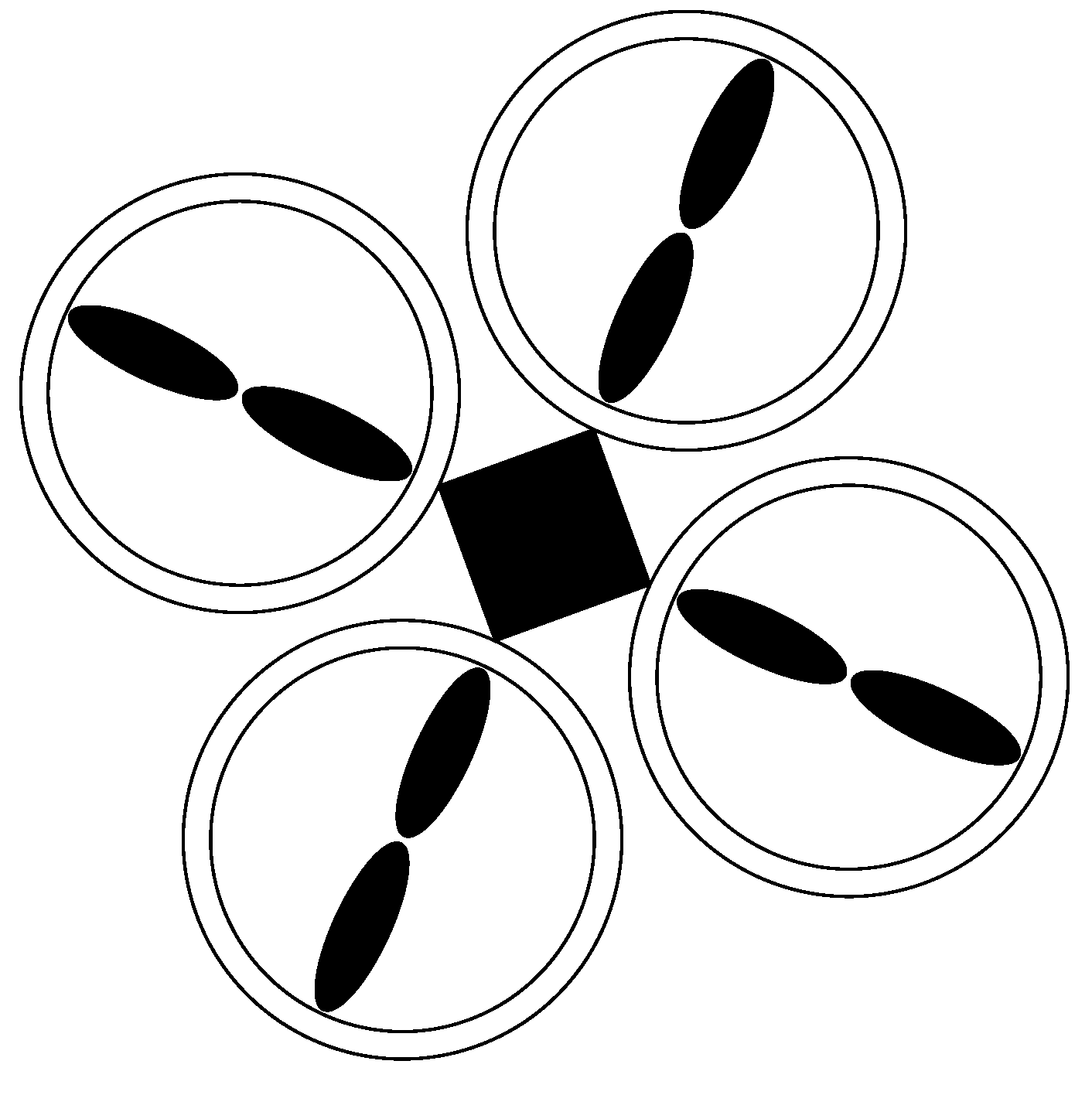
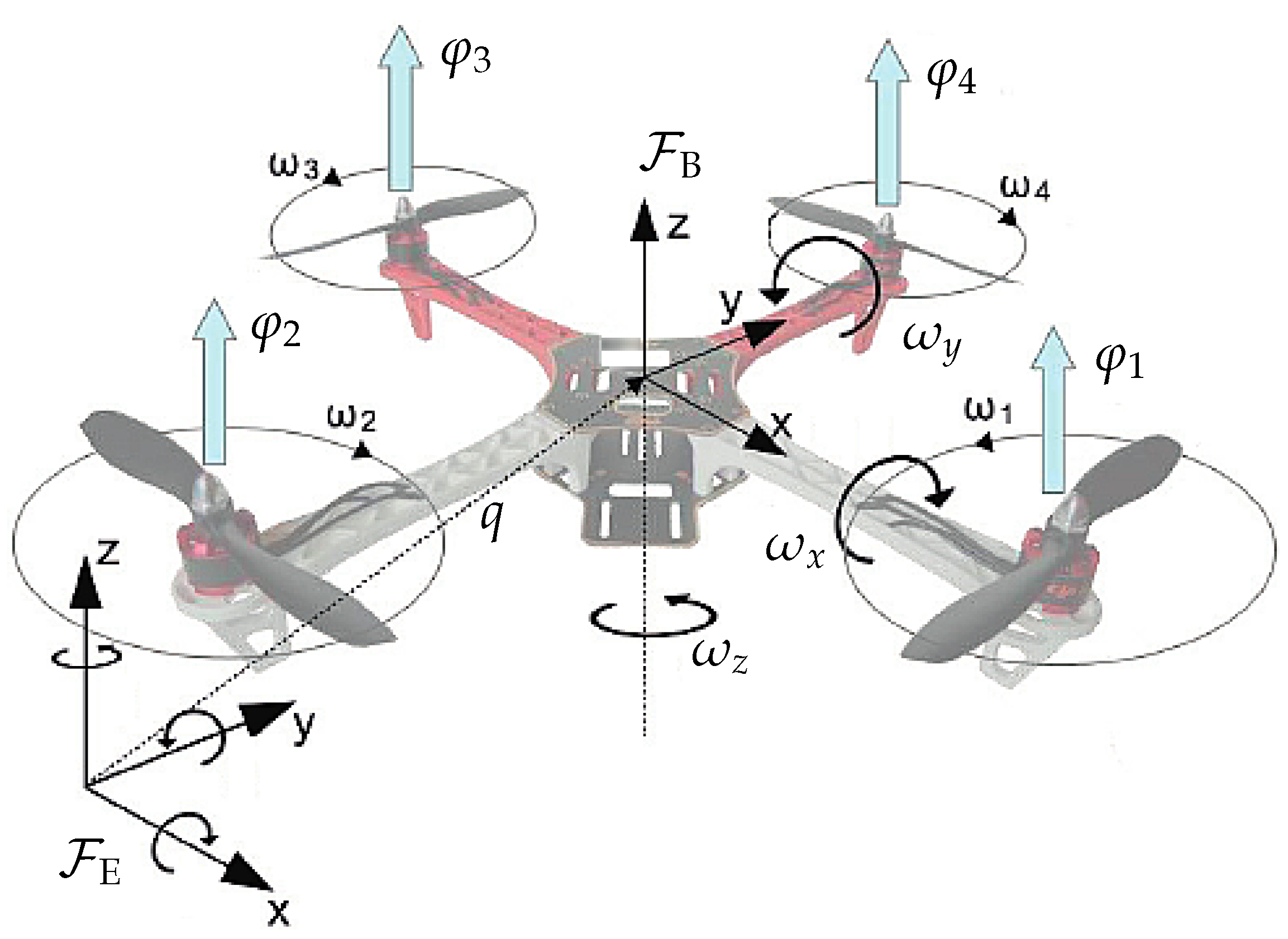
3.2. Quadrotor Drone

A quadrotor drone (also referred to as quadcopter [17,18,19]) is a helicopter with four rotors directed upwards and placed in a square formation with equal distance from the center, as in Figure 2. The quadrotor is controlled by adjusting the angular velocities of the rotors, which are responsible for both lift and propulsion. A horizontal movement is achieved by tilting the platform, while a vertical movement is achieved by changing the total thrust of the rotors [20].

Figure 2. A schematic quadrotor.

In the simplest model, as the one studied here, the only degrees of freedom are the velocity at which the four rotors spin. An unbalance in the spinning velocities of the propellers causes, in general, the platform to tilt (hence to change its attitude and to shift horizontally), to ascend or descend (that is, to shift vertically), and to spin along its vertical axis (which is referred to as yawing).

In general, a quadrotor model is written on the basis of the following assumptions: The structure is supposed to be rigid and axis-symmetrical, with the center of the axis coinciding with the center of mass, thrust and drag are proportional to the square of each rotor’s angular speed, and the rotors are supposed to be rigid. Further assumptions may be made to simplify the analytic treatment.

The quadrotor is made of a body $\mathcal{B}$ and of four rotors ${\mathcal{R}}_a$, with $a=1,2,3,4$, also termed propellers. We assume that one pair of propellers ($a=2$ and $a=4$) is rotating clockwise, while the other pair of propellers ($a=1$ and $a=3$) is rotating counterclockwise, as shown in Figure 3. The rotor ${\mathcal{R}}_1$ is located along the $+x$ axis (hence the rotor ${\mathcal{R}}_3$ is located along the $-x$ axis), while the rotor ${\mathcal{R}}_4$ is located along the $+y$ axis (hence the rotor ${\mathcal{R}}_2$ is located along the $-y$ axis). The coordinates of each volume element of the drone are referred to as an earth reference frame denoted by ${\mathcal{F}}_{\mathrm{E}}$. A reference frame, denoted as ${\mathcal{F}}_{\mathrm{B}}$, is attached to the body of the quadrotor, with the origin in its center of mass, as shown in Figure 3.

Figure 3. Quadcopter reference frames.

In the present subsection, as already done for the gyrostat satellite, we proceed on determining a model of quadcopter by a fully geometric approach, namely by means of the Euler–Poincaré equations written in compact form, without resorting to component-wise expressions or classical physics definitions. This procedure makes the system modeling more straightforward and, we believe, notationally easier to manage (compare, e.g., to a more classical procedure used in [21]).

3.2.1. Total Kinetic Energy

The position of the center of mass of the quadrotor with respect to an inertial reference frame ${\mathcal{F}}_{\mathrm{E}}$ is denoted by $q\in {\mathbb{R}}^3$. The orientation of a quadrotor-fixed reference frame ${\mathcal{F}}_{\mathrm{B}}$ with respect to the inertial reference frame ${\mathcal{F}}_{\mathrm{E}}$ is denoted by a rotation matrix $R\in \mathrm{SO}\left(3\right)$. The matrix R represents the rotation needed to align the orthogonal frame ${\mathcal{F}}_{\mathrm{B}}$ to the orthogonal frame ${\mathcal{F}}_{\mathrm{E}}$. A rotation around the x axis is termed roll, a rotation around the y axis is termed pitch and a rotation around the z axis is termed yaw. The matrix R changes over time according to the tilting of the quadrotor. When $R=I_3$, the quadcopter is perfectly horizontal and the reference frames are perfectly aligned.

Any volume element of mass $\mathrm{d}m$ within the body of the quadcopter is individuated by a coordinate $x=q+R{x}_0$ with respect to the earth reference frame ${\mathcal{F}}_{\mathrm{E}}$, where $x_0$ denotes the position of the volume element in the body-fixed reference frame ${\mathcal{F}}_{\mathrm{B}}$. The kinetic energy of the body is given by

$$k_{\mathrm{b}}:=\frac{1}{2}\underset{\mathcal{B}}{\int }\mathrm{tr}\left(\dot{x}{\dot{x}}^{\top }\right)\mathrm{d}m,$$

(77)

where $\dot{x}=\dot{q}+\dot{R}{x}_0$. The vector $\dot{q}$ denotes the linear velocity of the body center in the earth-fixed reference frame ${\mathcal{F}}_{\mathrm{E}}$. Recalling that $\dot{R}=R\xi$, it is not difficult to obtain the following expression for the kinetic energy of the body:

$$k_{\mathrm{b}}=\frac{1}{2}{M}_{\mathrm{b}}{\parallel \dot{q}\parallel }^2+\frac{1}{2}\mathrm{tr}\left(\xi {\widehat{J}}_{\mathrm{b}}{\xi }^{\top }\right)+M_{\mathrm{b}}\mathrm{tr}\left(\dot{q}{\overline{c}}_{\mathrm{b}}^{\top }{\dot{R}}^{\top }\right),$$

(78)

where

$$M_{\mathrm{b}}:=\underset{\mathcal{B}}{\int }\mathrm{d}m,{\widehat{J}}_{\mathrm{b}}:=\underset{\mathcal{B}}{\int }{x}_0{x}_0^{\top }\mathrm{d}m,{\overline{c}}_{\mathrm{b}}:=\frac{1}{M_{\mathrm{b}}}\underset{\mathcal{B}}{\int }{x}_0\mathrm{d}m.$$

(79)

The scalar quantity $M_{\mathrm{b}}$ denotes the total body mass and the $3\times 3$ matrix ${\widehat{J}}_{\mathrm{b}}$ denotes the non-standard inertia tensor of the quadcopter body. The vector ${\overline{c}}_{\mathrm{b}}\in {\mathbb{R}}^3$ denotes the position of the center of mass of the body in the body-fixed frame. By the assumptions made, it holds that ${\overline{c}}_{\mathrm{b}}=0$.

Next, we embody in the model the information that the four rotors are located at equal distance from the center of the body, two on the x axis and two on the y axis. A point on the rotor ${\mathcal{R}}_a$ has coordinates, in the inertial reference frame, given by

$$x=q+R(p_a+R_{a}s)\Rightarrow R^{\top }\dot{x}=R^{\top }\dot{q}+\xi p_a+(\xi +{\xi }_a)R_{a}s,$$

(80)

where q, $\dot{q}$ and R are defined as before, $p_a\in {\mathbb{R}}^3$ denotes the position of the rotor ${\mathcal{R}}_a$ with respect to the body-fixed frame, and $R_a\in \mathrm{SO}\left(3\right)$ denotes the instantaneous rotation of a rotor-fixed frame with respect to the body-fixed frame ${\mathcal{F}}_{\mathrm{B}}$; moreover, ${\dot{R}}_a={\xi }_a{R}_a$ (recall that $\frac{\mathrm{d}{p}_a}{\mathrm{d}t}=0$). Then, the kinetic energy of the rotor ${\mathcal{R}}_a$ is given by

$$k_a=\frac{1}{2}{M}_a{\parallel \dot{q}\parallel }^2+\frac{1}{2}\mathrm{tr}\left(\xi p_a{p}_a^{\top }{\xi }^{\top }\right)+\mathrm{tr}\left((\xi +{\xi }_a)R_a{\widehat{J}}_a{R}_a^{\top }{(\xi +{\xi }_a)}^{\top }\right)+M_a\mathrm{tr}\left(R^{\top }\dot{q}{p}_a^{\top }\xi \right),$$

(81)

where

$$M_a:=\underset{{\mathcal{R}}_a}{\int }\mathrm{d}m,{\widehat{J}}_a:=\underset{{\mathcal{R}}_a}{\int }{x}_0{x}_0^{\top }\mathrm{d}m,\underset{{\mathcal{R}}_a}{\int }s\mathrm{d}m=0,\sum _{a=1}^4{p}_a=0.$$

(82)

The last two equalities are due to symmetry of each rotor and to their symmetric disposition within the quadcopter body.

The total kinetic energy of the quadcopter is, thus, given by:

$$k:=k_{\mathrm{b}}+\sum _{a=1}^4{k}_a=\frac{1}{2}{M}_{\mathrm{q}}{\parallel \dot{q}\parallel }^2+\frac{1}{2}\mathrm{tr}\left(\xi \widehat{J}{\xi }^{\top }\right)+\frac{1}{2}\sum _{a=1}^4\mathrm{tr}\left((\xi +{\xi }_a){\widehat{J}}_a{(\xi +{\xi }_a)}^{\top }\right),$$

(83)

where

$$M_{\mathrm{q}}:=M_{\mathrm{b}}+\sum _{a=1}^4{M}_a,\widehat{J}:={\widehat{J}}_{\mathrm{b}}+\sum _{a=1}^4{M}_a{p}_a{p}_a^{\top }.$$

(84)

Notice that the rotors have been assumed symmetric with respect to the spin axis z, hence we exploited again the relation $R_a{\widehat{J}}_a{R}_a^{\top }={\widehat{J}}_a$.

3.2.2. Equations for the Rotational Component of Motion

Since all the rotors are spinning about the z axis, ${\xi }_a:={(-1)}^a{\omega }_a{\xi }_z$. In addition, we assume that all rotors have the same inertia tensor, therefore $\{{\widehat{J}}_a,{\xi }_a\}={(-1)}^a{\omega }_a{J}_{\mathcal{R}}{\xi }_z$, where $J_{\mathcal{R}}$ is a given constant. The factor ${(-1)}^a$ was introduced in the equations to take into account the fact that rotors ${\mathcal{R}}_1$ and ${\mathcal{R}}_3$ are spinning counterclockwise, while rotors ${\mathcal{R}}_2$ and ${\mathcal{R}}_4$ are spinning clockwise. In this manner, their angular velocities ${\omega }_1,{\omega }_2,{\omega }_3,{\omega }_4$ represent absolute speeds proportional to their RPM (revolutions per minute) rate.

In order to obtain equations that describe the rotational component of motion, we take $\ell \left(\xi \right):=k\left(\xi \right)$ and compute the fiber derivative:

$$\frac{\mathrm{d}\ell }{\mathrm{d}\xi }=\frac{1}{2}\{\widehat{J},\xi \}+\frac{1}{2}\sum _{a=1}^4\{{\widehat{J}}_a,\xi +{\xi }_a\}=\frac{1}{2}\{{\widehat{J}}_{\mathrm{q}},\xi \}+\frac{1}{2}\beta ,$$

(85)

where

$${\widehat{J}}_{\mathrm{q}}:=\widehat{J}+\sum _{a=1}^4{\widehat{J}}_a,\beta :=(-{\omega }_1+{\omega }_2-{\omega }_3+{\omega }_4)J_{\mathcal{R}}{\xi }_z.$$

(86)

Each rotor exerts a thrust ${\phi }_a\in {\mathbb{R}}^3$ along the z axis of the body-fixed reference frame (that is, a vertical force in the body-fixed frame ${\mathcal{F}}_{\mathrm{B}}$ that tends to push the quadrotor body upward), as shown in the Figure 3. The magnitude of the thrust generated by rotor ${\mathcal{R}}_a$ is proportional to ${\omega }_a^2$ via a lift constant denoted by $\frac{1}{2}b>0$, namely:

$${\phi }_1:=\frac{1}{2}b{\omega }_1^2{\mathrm{e}}_z,{\phi }_2:=\frac{1}{2}b{\omega }_2^2{\mathrm{e}}_z,{\phi }_3:=\frac{1}{2}b{\omega }_3^2{\mathrm{e}}_z,{\phi }_4:=\frac{1}{2}b{\omega }_4^2{\mathrm{e}}_z,with{\mathrm{e}}_z:=\left[\begin{array}{c}0\\ 0\\ 1\end{array}\right].$$

(87)

The lift constant is proportional to the air density and to the rotor cross-section. Each thrust ${\phi }_a$ is supposed to appear at the tip of each rotor, therefore its moment arm $p_a$ produces a mechanical torque on the body of the quadcopter, which has the effect of tilting the quadrotor drone with respect to the earth frame ${\mathcal{F}}_{\mathrm{E}}$ during flight. The four moment arms are given by

$$p_1:=\left[\begin{array}{c}r\\ 0\\ 0\end{array}\right],p_2:=\left[\begin{array}{c}0\\ r\\ 0\end{array}\right],p_3:=\left[\begin{array}{c}-r\\ 0\\ 0\end{array}\right],p_4:=\left[\begin{array}{c}0\\ -r\\ 0\end{array}\right].$$

(88)

Moreover, each rotor produces a drag torque, which is directed along the z axis and is proportional to the square angular velocity of each rotor through a drag constant $\frac{1}{2}\gamma >0$, namely ${\tau }_a:=\gamma {(-1)}^a{\omega }_a^2{\xi }_z$. A drag torque is present due to the spinning of each rotor which, by virtue of the angular momentum conservation law, will produce a counter torque that acts on the whole body of the quadcopter and tends to produce a rotation along its vertical axis.

Therefore, the total external torque acting on the quadcopter is

$$\tau :=\frac{1}{2}\sum _{a=1}^4{(-1)}^a({\phi }_a{p}_a^{\top }-p_a{\phi }_a^{\top })+\frac{\gamma }{2}\sum _{a=1}^4{(-1)}^a{\omega }_a^2{\xi }_z.$$

(89)

The external mechanical torque $\tau \in \mathfrak{so}\left(3\right)$ may be written in components with respect to the basis (21) as ${\tau }_x={\xi }_z+{\tau }_y{\xi }_y+{\tau }_z{\xi }_z$. By direct computations, it is found that

$$\left\{\begin{array}{c}{\tau }_x=br({\omega }_4^2-{\omega }_2^2),\hfill \\ {\tau }_y=br({\omega }_3^2-{\omega }_1^2),\hfill \\ {\tau }_z=\gamma (-{\omega }_1^2+{\omega }_2^2-{\omega }_3^2+{\omega }_4^2).\hfill \end{array}\right.$$

(90)

Therefore, the torque due to rotor thrusts has the effect of tilting the quadcopter body along the roll and the pitch axes, while the torque due to drag produces a rotation of the body around the yaw axis. It is worth remarking, taking as the reference Figure 3, that a positive rotation along the yaw axis coincides with the direction of rotation of rotors ${\mathcal{R}}_1$ and ${\mathcal{R}}_3$ and is opposite to the direction of rotation of rotors ${\mathcal{R}}_2$ and ${\mathcal{R}}_4$. The expression ${\tau }_z=\gamma ({\omega }_2^2+{\omega }_4^2)-\gamma ({\omega }_1^2+{\omega }_3^2)$ tells that the drag of rotors ${\mathcal{R}}_1$ and ${\mathcal{R}}_3$ tends to rotate the body of the quadcopter in a negative yaw direction, while the drag of rotors ${\mathcal{R}}_2$ and ${\mathcal{R}}_4$ tends to rotate the body of the quadcopter in a positive yaw direction. This sign inversion is due to the fact that, when an internal part tends to rotate in a given direction, the whole body tends to rotate in the opposite direction, because of the conservation of the total angular momentum.

In summary, the Euler–Poincaré equations (19) for the quadrotor drone read

$$\left\{\begin{array}{ccc}\dot{R}& =& R\xi ,\hfill \\ \{{\widehat{J}}_{\mathrm{q}},\dot{\xi }\}& =& [{\widehat{J}}_{\mathrm{q}},{\xi }^2]+[\beta ,\xi ]-\dot{\beta }+\tau ,\hfill \\ \beta & :=& (-{\omega }_1+{\omega }_2-{\omega }_3+{\omega }_4)J_{\mathcal{R}}{\xi }_z,\hfill \\ \tau & :=& br({\omega }_4^2-{\omega }_2^2){\xi }_x+br({\omega }_3^2-{\omega }_1^2){\xi }_y+\gamma (-{\omega }_1^2+{\omega }_2^2-{\omega }_3^2+{\omega }_4^2){\xi }_z.\hfill \end{array}\right.$$

(91)

The second equation (that expresses the dynamics of $\xi$) is much simpler than the equations of motion derived by using local coordinates (e.g., yaw, pitch and roll angles) because it is written with respect to a body-fixed frame ${\mathcal{F}}_{\mathrm{B}}$ and expressed in the Lie algebra $\mathfrak{so}\left(3\right)$ (compare, e.g., with [20]).

For completeness and easiness of comparison to other formulations, we report below the differential equations governing the evolution of the components ${\omega }_x,{\omega }_y,{\omega }_z$ of the angular tensor $\xi$:

$$\left\{\begin{array}{c}{\dot{\omega }}_x={\displaystyle \frac{J_y-J_z}{J_x}}{\omega }_y{\omega }_z-{\displaystyle \frac{J_{\mathcal{R}}}{J_x}}({\omega }_1-{\omega }_2+{\omega }_3-{\omega }_4){\omega }_y+{\displaystyle \frac{br}{J_x}}({\omega }_4^2-{\omega }_2^2),\hfill \\ {\dot{\omega }}_y={\displaystyle \frac{J_z-J_x}{J_y}}{\omega }_x{\omega }_z+{\displaystyle \frac{J_{\mathcal{R}}}{J_y}}({\omega }_1-{\omega }_2+{\omega }_3-{\omega }_4){\omega }_x+{\displaystyle \frac{br}{J_y}}({\omega }_3^2-{\omega }_1^2),\hfill \\ {\dot{\omega }}_z={\displaystyle \frac{J_x-J_y}{J_z}}{\omega }_x{\omega }_y-{\displaystyle \frac{J_{\mathcal{R}}}{J_z}}({\dot{\omega }}_1-{\dot{\omega }}_2+{\dot{\omega }}_3-{\dot{\omega }}_4)-{\displaystyle \frac{\gamma }{J_z}}({\omega }_1^2-{\omega }_2^2+{\omega }_3^2-{\omega }_4^2),\hfill \end{array}\right.$$

(92)

where $\mathrm{diag}(J_x,J_y,J_z)=J_{\mathrm{q}}$. Some comments on these equations are in order:

Rotors spinning velocities: the four rotors spin at almost constant velocity and do not change the spinning direction during operation. Their spinning velocity changes only slightly, namely to ${\omega }_a\pm \mathsf{\Delta }{\omega }_a$, in order to create a slight unbalance in the thrusts that produces a slight tilting and affords controlling the attitude/tilt of the body. The quantity ${\mathsf{\Omega }}_r:={\omega }_1-{\omega }_2+{\omega }_3-{\omega }_4$ is termed residual rotoric angular velocity and the quantity $J_{\mathcal{R}}{\dot{\mathsf{\Omega }}}_r$ is termed inertial counter-torque [22].

Independence from attitude: the equation $\{{\widehat{J}}_{\mathrm{q}},\dot{\xi }\}=[{\widehat{J}}_{\mathrm{q}},{\xi }^2]+[\beta ,\xi ]-\dot{\beta }+\tau$ governs the body rotation velocity (in terms of rotation speed and direction). This equation is independent of the current attitude R of the body itself. In fact, the matrix R does not appear in this equation.

In steady state flight (i.e., not takeoff or landing), the term $J_{\mathcal{R}}{\dot{\mathsf{\Omega }}}_r$ is unessential because ${\mathsf{\Omega }}_r$ is kept constant, since most of the time the rotors will be maintaining an almost constant thrust and will not be accelerating. Moreover, due to the symmetry of the quadrotor, one may take $J_y\equiv J_x$. With these assumptions, the model simplifies to

$$\begin{array}{ccc}\hfill {\dot{\omega }}_x& =& \frac{J_x-J_z}{J_x}{\omega }_y{\omega }_z-\frac{J_{\mathcal{R}}}{J_x}{\mathsf{\Omega }}_r{\omega }_y+\frac{br}{J_x}({\omega }_4^2-{\omega }_2^2),\hfill \end{array}$$

(93)

$$\begin{array}{ccc}\hfill {\dot{\omega }}_y& =& \frac{J_z-J_x}{J_x}{\omega }_x{\omega }_z+\frac{J_{\mathcal{R}}}{J_y}{\mathsf{\Omega }}_r{\omega }_x+\frac{br}{J_y}({\omega }_3^2-{\omega }_1^2),\hfill \end{array}$$

(94)

$$\begin{array}{ccc}\hfill {\dot{\omega }}_z& =& -\frac{\gamma }{J_z}({\omega }_1^2-{\omega }_2^2+{\omega }_3^2-{\omega }_4^2).\hfill \end{array}$$

(95)

The global spinning motion around the z axis is due only to drag. Since the propellers ${\mathcal{R}}_2$ and ${\mathcal{R}}_4$ are rotating clockwise, while the propellers ${\mathcal{R}}_1$ and ${\mathcal{R}}_3$ are rotating counterclockwise, the Equation (95) tells us that the net difference between the clockwise-directed angular velocities and the counterclockwise-directed angular velocities produces a counterclockwise spinning of the body of the drone.

3.2.3. Equations for the Translational Component of Motion

The translation component of motion obeys the Newton’s law written in the inertial (earth) reference frame ${\mathcal{F}}_{\mathrm{E}}$, namely, the linear acceleration $\ddot{q}$ is proportional to the total thrust ${\phi }_{\mathrm{T}}:={\sum }_{a=1}^4{\phi }_a$, to the gravity acceleration and to an aerodynamic drag term. Notice that the vector ${\phi }_{\mathrm{T}}$ is directed along the constant direction ${\mathrm{e}}_z$ in the body-fixed reference frame ${\mathcal{F}}_{\mathrm{B}}$ which, in turn, is rotated of a quantity R with respect to the earth frame ${\mathcal{F}}_{\mathrm{E}}$, therefore, in the earth-fixed frame, the total thrust is directed along the rotated axis $R·{\mathrm{e}}_z$. Formally, the just-recalled Newton’s law is written as:

$$M_{\mathrm{q}}\ddot{q}=\frac{1}{2}b({\omega }_1^2+{\omega }_2^2+{\omega }_3^2+{\omega }_4^2)R{\mathrm{e}}_z-M_{\mathrm{q}}p{\mathrm{e}}_z-\mathsf{\Gamma }\dot{q},$$

(96)

where $p$ denotes the gravitational acceleration scalar and Γ ∈ ${\mathbb{R}}^{3\times 3}$ denotes an aerodynamic drag tensor (typically, diagonal).

Whenever the quadcopter is in a horizontal position, namely $R=I_3$, its center of mass can only move vertically (the thrust is directed along ${\mathrm{e}}_z$). Whenever the quadcopter is tilted, namely $R{\mathrm{e}}_z-\left({\mathrm{e}}_z^{\top }R{\mathrm{e}}_z\right){\mathrm{e}}_z\ne 0$, then the quadcopter changes direction.

3.2.4. Explicit State-Space Form of Quadcopter Equations

By adopting again the concept introduced in the Section 3.1.5, that is $\{{\widehat{J}}_{\mathrm{q}},\dot{\xi }\}=D\dot{\xi }D$, where the matrix D is defined as in (72), we may rewrite the set of equations governing the flight of a quadcopter drone as

$$\left\{\begin{array}{ccc}\dot{R}& =& R\xi ,\hfill \\ \dot{\xi }& =& D^{-1}([{\widehat{J}}_{\mathrm{q}},{\xi }^2]+[\beta ,\xi ]-\dot{\beta }+\tau )D^{-1},\hfill \\ \beta & :=& (-{\omega }_1+{\omega }_2-{\omega }_3+{\omega }_4)J_{\mathcal{R}}{\xi }_z,\hfill \\ \tau & :=& br({\omega }_4^2-{\omega }_2^2){\xi }_x+br({\omega }_3^2-{\omega }_1^2){\xi }_y+\gamma (-{\omega }_1^2+{\omega }_2^2-{\omega }_3^2+{\omega }_4^2){\xi }_z,\hfill \\ \dot{q}& =& v,\hfill \\ \dot{v}& =& \frac{1}{2}\frac{b}{M_{\mathrm{q}}}({\omega }_1^2+{\omega }_2^2+{\omega }_3^2+{\omega }_4^2)R{\mathrm{e}}_z-p{\mathrm{e}}_z-\frac{1}{M_{\mathrm{q}}}\mathsf{\Gamma }v.\hfill \end{array}\right.$$

(97)

For exemplary values of the parameters (OS4 Mini-VTOL quadrotor model), interested readers might want to consult [22]. The model (95) does not include a number of physical effects, such as hub moment and rolling moment due to sideward/forward flight, nor a sub-model of the brushless direct-current motor and of the gearbox.

4. Numerical Integration of Initial Value Problems

We focus on dynamical systems of the first order, namely initial value problems [23], since it is always possible to reformulate a dynamical system of higher order into a dynamical system of first order by augmenting the number of variables. We start off by recalling two numerical methods for initial value problems on ${\mathbb{R}}^n$. The reason for this choice is twofold: the methods on ${\mathbb{R}}^n$ may be generalized to numerical methods on manifolds and Lie groups by appropriate analysis techniques [24], for example to integrate the equations that govern the rotational component of motion; in addition, the equations that govern the translation component of motion need numerical methods on ${\mathbb{R}}^3$.

4.1. Numerical Schemes in ${\mathbb{R}}^n$

Classical initial-value problems have the Euclidean space ${\mathbb{R}}^n$ as domain [25,26]. Well-known numerical integration techniques used in engineering and in applied sciences are the forward Euler method and the explicit fourth-order Runge–Kutta method. The original Euler’s method [27] exhibits a good behavior as a numerical integration method and can be used to study a number of important phenomena [28]. The Euler method is traditionally the first numerical technique introduced to solve initial value problems. It is simple to understand and geometrically easy to articulate, but it is known to show limited accuracy for complicated functions. A more robust and intricate family of numerical integration method is the Runge–Kutta scheme. This method is the most widely used one since it gives reliable results and is particularly suitable when the computation of higher derivatives is unpractical. An account for the whole spectrum of both stiff and non-stiff ordinary differential equations solvers is provided by [29,30]. A classical account of Runge–Kutta methods was given in the monograph [31] and in the textbooks on ordinary differential equations [28,32,33].

In addition to Runge–Kutta and linear multi-step methods, Taylor series methods may be considered as a third main direction of development. These three main classes of numerical ordinary differential equations solvers have, respectively, the characteristic of using more derivatives. A variety of new numerical schemes can be constructed which are combinations of methods from the three main classes. An important class of such new schemes consists of the multi-stage multi-step methods known as multi-step Runge–Kutta methods [32]. Another class of numerical schemes is formed by the multi-step-multi-derivative methods, known as Obreshkov methods [34]. The Kutta–Merson method [35] belongs to the family of so-called embedded Runge–Kutta methods. These schemes are useful because they provide a tool by which the accuracy of the calculations can be monitored during the integration process, but they are also quite burdensome to implement on a computing platform.

A generic first-order, non-autonomous, dynamical system whose state variable is denoted by $x\in {\mathbb{R}}^n$ may be written as

$$\dot{x}=\sigma (x,t),\mathrm{with}x\left(0\right)=x_0,t>0,$$

(98)

where the function $\sigma :{\mathbb{R}}^n\times \mathbb{R}\to {\mathbb{R}}^n$ describes completely the dynamical system. In calculus, the above system is referred to as an “initial value problem” which may be solved under mild regularity conditions. The variable $x\in {\mathbb{R}}^n$ represents the state of the dynamical system, while its derivative with respect to the time, $\dot{x}$, denotes the state speed. We notice here that, incidentally, while x and $\dot{x}$ possess a rather different physical meaning (for example, position and speed, respectively, of a particle) they belong to the same space ${\mathbb{R}}^n$. This is, indeed, rather a special case, since systems whose state evolve on curved spaces do not enjoy this property. We also observe that the explicit dependence of the state-transition function $\sigma$ from the parameter t (which, in most applications, represent time), serves to summarize the possible dependence of $\sigma$ from a number of time-varying external sources of information (for example, a linear input-state system may be represented by a differential equation like (98) by setting $\sigma (x,t):=Ax+Bu\left(t\right)$, where $u\left(t\right)$ denotes a time-varying input signal). In most of the cases of interest in applied sciences, problem (98) is not tractable analytically and needs to be solved numerically.

In the following subsubsections, we recall from the scientific literature two of the above-mentioned numerical integration schemes, namely the forward Euler scheme and the explicit fourth-order Runge–Kutta scheme and illustrate their behavior on the numerical simulation of a non-linear, chaotic system. Although both methods are most likely well-known to the readers, we believe that it is important to briefly recall their essential features in view of their extension from the space ${\mathbb{R}}^n$ to curved manifolds, which will be pursued in the next subsection.

4.1.1. Forward Euler Scheme

The forward Euler scheme [36] (hereafter denoted by fEul), is perhaps the simplest (yet effective) numerical integration scheme for an initial value problem known in the scientific literature. It is based on two key ideas, namely, the uniform time-discretization of the state variable and the approximation of its first-order derivative by means of the right-side incremental ratio.

Uniform time-discretization is a procedure that affords switching from a continuous function of a temporal variable to a succession. In other terms, since we are unable to evaluate the state $x\left(t\right)$ at any time, we define a uniform succession of time-steps, separated by a reasonably short interval $T>0$ termed stepsize, which are denoted by $t_0=0$, $t_1=t_0+T$, $t_2=t_1+T$, and so forth, at which we will try to approximate the values of the state. The fEul scheme is based on the approximation

$$\dot{x}\left(t\right)={\displaystyle \frac{x(t+T)-x\left(t\right)}{T}}+\epsilon \left(t\right),$$

(99)

where $\epsilon \in {\mathbb{R}}^n$ denotes an error term. Plugging the above approximation into the equation of the dynamical system (98) and applying a uniform time-discretization, we obtain:

$$T\sigma (x\left(t_k\right),t_k)=x\left(t_{k+1}\right)-x\left(t_k\right)+T\epsilon \left(t_k\right),k=1,2,3,\dots .$$

(100)

The fEul numerical integration scheme arises by ignoring the error term and by replacing the actual values of the state by their approximations, which are denoted by $x_1$, $x_2$, $x_3$ and so forth. The magnitude $\parallel \epsilon \left(t_k\right)\parallel$ of the error at every step determines the precision of the numerical scheme. The approximations are calculated iteratively by the numerical scheme

$$x_{k+1}=x_k+T\sigma (x_k,t_k),k=1,2,3,\dots .$$

(101)

The error in this method is as small as $T^2$. The number of steps depends on the discretization step-size and on the extension of the time-interval that a solution is sought within. Namely, if $t\in [t_0,t_{\mathrm{f}}]$, then the number of steps is the nearest integer to the ratio $(t_{\mathrm{f}}-t_0)/T$.

4.1.2. Explicit Fourth-Order Runge–Kutta Scheme on ${\mathbb{R}}^n$

The family of Runge–Kutta numerical integration schemes [36] was developed to increase the precision of the solution and is based on the evaluation of the function f at a number of locations in the interval $[t_k,t_{k+1}]$. In particular, the explicit fourth-order Runge–Kutta scheme (hereafter denoted as eRK4), is based on four partial increments that, added together, bring to a complete step. The eRK4 approximation of the actual solution to the initial value problem (98) may be expressed by the following equations:

$$\left\{\begin{array}{c}{H}_1\left(t_k\right)=\sigma (x\left(t_k\right),t_k),\hfill \\ H_2\left(t_k\right)=\sigma (x\left(t_k\right)+\frac{1}{2}T{H}_1\left(t_k\right),t_k+\frac{1}{2}T),\hfill \\ H_3\left(t_k\right)=\sigma (x\left(t_k\right)+\frac{1}{2}T{H}_2\left(t_k\right),t_k+\frac{1}{2}T),\hfill \\ H_4\left(t_k\right)=\sigma (x\left(t_k\right)+T{H}_3\left(t_k\right),t_k+T),\hfill \\ x\left(t_{k+1}\right)=x\left(t_k\right)+T(\frac{H_1\left(t_k\right)}{6}+\frac{H_2\left(t_k\right)+H_3\left(t_k\right)}{3}+\frac{H_4\left(t_k\right)}{6})+{\epsilon }^{\prime }\left(t_k\right),\hfill \end{array}\right.$$

(102)

for $k=0,1,2,3,\dots$. Once again, by ignoring the error term and by denoting the approximations of the state at step k by $x_k$, we get the eRK4 scheme:

$$\left\{\begin{array}{c}{H}_{1,k}=\sigma (x_k,t_k),\hfill \\ H_{2,k}=\sigma (x_k+\frac{1}{2}T{H}_{1,k},t_k+\frac{1}{2}T),\hfill \\ H_{3,k}=\sigma (x_k+\frac{1}{2}T{H}_{2,k},t_k+\frac{1}{2}T),\hfill \\ H_{4,k}=\sigma (x_k+T{H}_{3,k},t_k+T),\hfill \\ x_{k+1}=x_k+T(\frac{H_{1,k}}{6}+\frac{H_{2,k}+H_{3,k}}{3}+\frac{H_{4,k}}{6}),\hfill \\ k=0,1,2,3,\dots .\hfill \end{array}\right.$$

(103)

Notice that $x_k,H_{1,k},H_{2,k},H_{3,k},H_{4,k},x_{k+1}$ all belong to the Euclidean space ${\mathbb{R}}^n$. This is not going to be the case when we will deal with curved manifolds rather than a Euclidean space ${\mathbb{R}}^n$. With reference to the interval $[t_k,t_{k+1}]$, the eRK4 method advances the solution from the step k to the step $k+1$ by combining together four estimations of the vector field $\sigma$ at four specific points, namely, once at the left-hand side of the interval ($H_{1,k}$), twice at the middle of the interval ($H_{2,k}$ and $H_{3,k}$), and once at the right-hand side of the interval ($H_{4,k}$). The stepping direction is a linear combination of these partial estimates whose coefficients are carefully crafted so as to ensure the error to be as small as $T^5$.

4.2. Extension of fEul and eRK4 Schemes to Smooth Manifolds

A dynamical system that has a smooth manifold $\mathbb{G}$ (which includes Lie groups) as state space is described by

$$\dot{g}=\sigma (g,t),g\left(0\right)=g_0\in \mathbb{G},$$

(104)

where $\sigma :\mathbb{G}\times \mathbb{R}\to T\mathbb{G}$. In fact, notice that, by definition of tangent space, it holds that $\dot{g}\in T_g\mathbb{G}$, therefore $\sigma (g,t)\in T_g\mathbb{G}$. This circumstance makes a significant difference in the numerical integration of problem (104) because, now, the system state and its first-order derivative no longer belong to the same space and, in addition, the state-space is no longer flat, which makes most of the operations listed in schemes (101) and (103) invalid.

The extension of the integration schemes to smooth manifolds is based on two key concept from differential geometry, namely, manifold retraction and parallel transport, which are surveyed briefly to clarify the notation [2,3] (see also [4,5] for a non-mathematical standpoint):

Manifold retraction: a map $\mathrm{Ret}:T\mathbb{G}\to \mathbb{G}$ is an operator that maps a pair $(g,\xi )\in T\mathbb{G}$ into a point in the manifold $\mathbb{G}$. The notation used within the present manuscript is $h={\mathrm{Ret}}_g\left(\xi \right)$ which indicates that it takes a point $g\in \mathbb{G}$, a tangent vector $\xi \in T_g\mathbb{G}$ and returns a point $h\in \mathbb{G}$. A manifold retraction is a generalization of a manifold exponential map and, as such, it shares zeroth- and first-order features, namely, ${\mathrm{Ret}}_g\left(0\right)=g$ and ${\left.\frac{d}{dt}{\mathrm{Ret}}_g\left(t\xi \right)\right|}_{t=0}=\xi$. In the case of a flat space ${\mathbb{R}}^n$ endowed with a Euclidean metric, the geodesic connecting any two points is a straight line and the retraction is given by ${\mathrm{Ret}}_g\left(\xi \right)=g+\xi$.

Parallel transport operator: a map $\mathrm{Par}:T\mathbb{G}\times \mathbb{G}\to T\mathbb{G}$ maps a tangent vector $\xi$ at a given point g on a manifold into a tangent vector at another given point h on the same manifold. The notation used within the present manuscript is $\eta ={\mathrm{Par}}_h^g\left(\xi \right)$ where $(g,\xi )\in T\mathbb{G}$ and $(h,\eta )\in T\mathbb{G}$. Parallel transport is a generalization of rigid translation of free vectors in ${\mathbb{R}}^n$ and ${\mathrm{Par}}_h^g$ is a linear isomorphism between $T_g\mathbb{G}$ and $T_h\mathbb{G}$ as well as an isometry. The above notation tacitly subsumes that the manifold $\mathbb{G}$ is endowed with a connection, hence geodesics, in such a way the operator $\mathrm{Par}$ transports the vector $\xi$ along the geodesic arc connecting points $g,h$ to give the new tangent vector $\eta$. In the case of a flat space ${\mathbb{R}}^n$ endowed with a Euclidean metric, parallel transport is given simply by $\eta =\xi$.

4.2.1. Forward Euler Scheme on a Smooth Manifold $\mathbb{G}$

As a first step, we replace the continuous trajectory $t\mapsto g\left(t\right)\in \mathbb{G}$ with the sequence $k\mapsto g_k\in \mathbb{G}$ and denote, for simplicity, ${\xi }_k:=\sigma (g_k,t_k)$.

It would be very convenient to approximate the solution of the dynamical system (104) by means of a fEul scheme like $x_{k+1}=x_k+T\sigma (x_k,t_k)$. However, even if we consider $\mathbb{G}$ as embedded in a larger Euclidean space, we quickly recognize that, on a curved manifold, the sum operation is not necessarily legitimate, namely, even though $g_k\in \mathbb{G}$ and ${\xi }_k\in T_{g_k}\mathbb{G}$, their linear combination $g_{k+1}=g_k+T{\xi }_k$ would result in a point laying outside of the manifold ($g_{k+1}\notin \mathbb{G}$). A way to extend a forward Euler stepping method is to replace addition with retraction, which leads to the following forward Euler scheme on manifold (hereafter referred to as fEulM):

$$g_{k+1}={\mathrm{Ret}}_{g_k}\left(T\sigma (g_k,t_k)\right),k=0,1,2,3,\dots ,K.$$

(105)

The above iterative scheme computes the first K points of the trajectory of the dynamical system (104) spaced apart of T in time.

4.2.2. Explicit Fourth-Order Runge–Kutta Scheme on a Smooth Manifold $\mathbb{G}$

Likewise, our extension of the explicit fourth-order Runge–Kutta method eRK4 to a manifold is based on the replacement of linear operations by retraction and parallel transport to give an explicit fourth-order Runge–Kutta method on manifold (hereafter denoted as eRK4M).

As a first step, we recall from scheme (103) that it is necessary to define four interlaced stages ${\xi }_{1,k},\dots ,{\xi }_{4,k}$ to advance the solution from the point $t_k$ to the point $t_{k+1}$. The four stages are outlines as follows:

• The first stage of the eRK4 scheme is defined as $H_{1,k}:=T\sigma (x_k,t_k)$. We can extend this calculation directly to a smooth manifold $\mathbb{G}$ to get the first stage of the eRK4M scheme by ${\xi }_{1,k}:=T\sigma (g_k,t_k)$. Notice that ${\xi }_{1,k}\in T_{g_k}\mathbb{G}$. The tangent vector ${\xi }_{1,k}$ represents an estimation of the tangent vector field $\sigma$ at $t_k$.
• The second stage of the eRK4 scheme is defined as $H_{2,k}:=T\sigma (x_k+\frac{1}{2}{H}_{1,k},t_k+\frac{1}{2}T)$. As we already know, the inner sum $x_k+\frac{1}{2}{H}_{1,k}$ is not necessarily legitimate on a manifold but may be extended by means of a retraction operator as ${\mathrm{Ret}}_{g_k}\left(\frac{1}{2}{\xi }_{1,k}\right)$. Therefore, we define the second stage of a eRK4M scheme as

  $${\xi }_{2,k}:=T\sigma ({\mathrm{Ret}}_{g_k}\left(\frac{1}{2}{\xi }_{1,k}\right),t_k+\frac{1}{2}T).$$

  (106)
  The tangent vector ${\xi }_{2,k}$ represents an estimation of the tangent vector field $\sigma$ at the midpoint $t_k+\frac{T}{2}$.
• The third stage of the eRK4 scheme is defined as $H_{3,k}:=T\sigma (x_k+\frac{1}{2}{H}_{2,k},t_k+\frac{1}{2}T)$. Now, this definition cannot be made legitimate just by replacing the inner sum with a retraction because ${\xi }_{2,k}\notin T_{g_k}\mathbb{G}$. Before applying a retraction, it is necessary to take a preliminary step, namely, to transport the local estimation of the vector field $\sigma$ to the space $T_{g_k}\mathbb{G}$. For the sake of notation conciseness, let us define the intermediate point

  $$g_{k+1/4}:={\mathrm{Ret}}_{g_k}\left(\frac{1}{2}{\xi }_{1,k}\right)$$

  (107)

  (the notation $k+1/4$ for the subscript is standard in numerical calculus). Notice now that ${\xi }_{2,k}\in T_{g_{k+1/4}}\mathbb{G}$. The third stage in the eRK4M scheme is defined as

  $${\xi }_{3,k}:=T\sigma ({\mathrm{Ret}}_{g_k}\left({\mathrm{Par}}_{g_k}^{g_{k+1/4}}\left(\frac{1}{2}{\xi }_{2,k}\right)\right),t_k+\frac{1}{2}T).$$

  (108)
  The tangent vector ${\xi }_{3,k}$ represents a further estimation of the tangent vector field $\sigma$ at the midpoint $t_k+\frac{T}{2}$, as required by the original eRK4 scheme.
• The fourth stage of the eRK4 scheme is defined as $H_{4,k}:=T\sigma (x_k+h_{3,k},t_k+T)$. Again, before applying a retraction, it is necessary to transport the local estimation of the vector field $\sigma$ to the space $T_{g_k}\mathbb{G}$. Let us define the intermediate point

  $$g_{k+1/2}:={\mathrm{Ret}}_{g_k}\left({\mathrm{Par}}_{g_k}^{g_{k+1/4}}\left(\frac{1}{2}{\xi }_{2,k}\right)\right)$$

  (109)

  and notice that ${\xi }_{3,k}\in g_{k+1/2}$. The fourth stage in the eRK4M scheme is defined as

  $${\xi }_{4,k}:=T\sigma ({\mathrm{Ret}}_{g_k}\left({\mathrm{Par}}_{g_k}^{g_{k+1/2}}\left({\xi }_{3,k}\right)\right),t_k+T).$$

  (110)
• In the original eRK4 scheme, the four stages $H_{1,k},\dots ,H_{4,k}$ are combined together as $x_{k+1}=x_k+T(\frac{H_{1,k}}{6}+\frac{H_{2,k}+H_{3,k}}{3}+\frac{H_{4,k}}{6})$. We already know that, on a curved manifold, the four stages belong to different tangent spaces and cannot, therefore, be combined together as they stand. In particular, the second increment needs to be transported to the tangent space $T_{g_k}\mathbb{G}$ by means of parallel transport to give ${\tilde{\xi }}_{2,k}:={\mathrm{Par}}_{g_k}^{g_{k+1/4}}\left({\xi }_{2,k}\right)$, the third stage needs to be replaced by ${\tilde{\xi }}_{3,k}:={\mathrm{Par}}_{g_k}^{g_{k+1/2}}\left({\xi }_{3,k}\right)$, and the fourth stage by ${\tilde{\xi }}_{4,k}:={\mathrm{Par}}_{g_k}^{g_{k+3/4}}\left({\xi }_{4,k}\right)$, where $g_{k+3/4}:={\mathrm{Ret}}_{g_k}\left({\mathrm{Par}}_{g_k}^{g_{k+1/2}}\left({\xi }_{3,k}\right)\right)$. The four stages ${\xi }_{1,k},{\tilde{\xi }}_{2,k},{\tilde{\xi }}_{3,k},{\tilde{\xi }}_{4,k}\in T_{g_k}\mathbb{G}$ may be combined together with the retraction map to give the next point in the sequence as

  $$g_{k+1}={\mathrm{Ret}}_{g_k}\left(\frac{{\xi }_{1,k}}{6}+\frac{{\tilde{\xi }}_{2,k}+{\tilde{\xi }}_{3,k}}{3}+\frac{{\tilde{\xi }}_{4,k}}{6}\right).$$

  (111)

In summary, the above stages and stepping equations may be recapitulated as:

$$\left\{\begin{array}{c}{\xi }_{1,k}=T\sigma (g_k,t_k),\hfill \\ g_{k+1/4}={\mathrm{Ret}}_{g_k}\left(\frac{1}{2}{\xi }_{1,k}\right),{\xi }_{2,k}=T\sigma (g_{k+1/4},t_k+\frac{1}{2}T),{\tilde{\xi }}_{2,k}={\mathrm{Par}}_{g_k}^{g_{k+1/4}}\left({\xi }_{2,k}\right),\hfill \\ g_{k+1/2}={\mathrm{Ret}}_{g_k}\left(\frac{1}{2}{\tilde{\xi }}_{2,k}\right),{\xi }_{3,k}=T\sigma (g_{k+1/2},t_k+\frac{1}{2}T),{\tilde{\xi }}_{3,k}={\mathrm{Par}}_{g_k}^{g_{k+1/2}}\left({\xi }_{3,k}\right),\hfill \\ g_{k+3/4}={\mathrm{Ret}}_{g_k}\left({\tilde{\xi }}_{3,k}\right),{\xi }_{4,k}=T\sigma (g_{k+3/4},t_k+T),{\tilde{\xi }}_{4,k}={\mathrm{Par}}_{g_k}^{g_{k+3/4}}\left({\xi }_{4,k}\right),\hfill \\ g_{k+1}={\mathrm{Ret}}_{g_k}\left(\frac{1}{6}{\xi }_{1,k}+\frac{1}{3}({\tilde{\xi }}_{2,k}+{\tilde{\xi }}_{3,k})+\frac{1}{6}{\tilde{\xi }}_{4,k}\right),\hfill \end{array}\right.$$

(112)

with $k=0,1,2,3,\dots ,K$. In the second, third and fourth equation, we encounter a compound function made of the parallel transport operator and of the vector field $\sigma$. Notation-wise (if not computation-wise), it is convenient to compose the two operators $\mathrm{Par}$ and $\sigma$ and to define the new operator

$$\mathrm{Par}{\sigma }_h^g\left(t\right):=T{\mathrm{Par}}_h^g\left(\sigma (g,t)\right).$$

(113)

Notice that the new operator $\mathrm{Par}\sigma$ encapsulates the step-size T. In summary, the eRK4M method may be expressed in the compact form:

$$\left\{\begin{array}{c}{\xi }_{1,k}=T\sigma (g_k,t_k),\hfill \\ g_{k+1/4}={\mathrm{Ret}}_{g_k}\left(\frac{1}{2}{\xi }_{1,k}\right),{\tilde{\xi }}_{2,k}=\mathrm{Par}{\sigma }_{g_k}^{g_{k+1/4}}(t_k+\frac{1}{2}T),\hfill \\ g_{k+1/2}={\mathrm{Ret}}_{g_k}\left(\frac{1}{2}{\tilde{\xi }}_{2,k}\right),{\tilde{\xi }}_{3,k}=\mathrm{Par}{\sigma }_{g_k}^{g_{k+1/2}}(t_k+\frac{1}{2}T),\hfill \\ g_{k+3/4}={\mathrm{Ret}}_{g_k}\left({\tilde{\xi }}_{3,k}\right),{\tilde{\xi }}_{4,k}=\mathrm{Par}{\sigma }_{g_k}^{g_{k+3/4}}(t_k+T),\hfill \\ g_{k+1}={\mathrm{Ret}}_{g_k}\left(\frac{1}{6}{\xi }_{1,k}+\frac{1}{3}({\tilde{\xi }}_{2,k}+{\tilde{\xi }}_{3,k})+\frac{1}{6}{\tilde{\xi }}_{4,k}\right),\hfill \end{array}\right.$$

(114)

with $k=0,1,2,3,\dots ,K$. A further observation is that the intermediate points $g_{k+1/4}$, $g_{k+1/2}$ and $g_{k+3/4}$ serve only to compute the tangent-vector stages, therefore it could be convenient to compactify even further the notation by introducing the operator

$$\mathrm{Par}\sigma {\mathrm{Ret}}_g(\xi ,t):=T{\mathrm{Par}}_g^{{\mathrm{Ret}}_g\left(\xi \right)}\left(\sigma (g,t)\right).$$

(115)

Through this compound operator, by adapting slightly the definitions of the ${\xi }_{i,k}$ to accommodate the new notation, the eRK4M method may be expressed as:

$$\left\{\begin{array}{c}{\xi }_{1,k}=\frac{1}{2}T\sigma (g_k,t_k),\hfill \\ {\xi }_{2,k}=\frac{1}{2}\mathrm{Par}\sigma {\mathrm{Ret}}_{g_k}({\xi }_{1,k},t_k+\frac{1}{2}T),\hfill \\ {\xi }_{3,k}=\mathrm{Par}\sigma {\mathrm{Ret}}_{g_k}({\xi }_{2,k},t_k+\frac{1}{2}T),\hfill \\ {\xi }_{4,k}=\mathrm{Par}\sigma {\mathrm{Ret}}_{g_k}({\xi }_{3,k},t_k),\hfill \\ g_{k+1}={\mathrm{Ret}}_{g_k}\left(\frac{1}{3}{\xi }_{1,k}+\frac{2}{3}{\xi }_{2,k}+\frac{1}{3}{\xi }_{3,k}+\frac{1}{6}{\xi }_{4,k}\right),\hfill \end{array}\right.$$

(116)

with $k=0,1,2,3,\dots ,K$ and $g_0\in \mathbb{G}$ given as initial point.

It is worth noticing here that the initial value problem might be more complex than Equation (104), as the vector field $\sigma$ might depend on other variables whose estimation, at midpoints, would then be necessary. This is the case, in fact, of rigid-body equations, which is tackled specifically in Section 5.

5. Numerical Integration of Rigid-Body Equations

The present section shows application of the numerical recipes to integrate first-order dynamical systems developed in the Section 4 to integrate the rigid-body equations recalled in the Section 3. In particular, we consider the numerical integration of a gyrostat satellite equations as well as of a quadrotor drone equations.

In order to put into effect the numerical schemes of Section 4.2, we choose as metric for the rotation group the canonical inner product, which leads to the following expressions for a retraction map (taken as the manifold exponential map arising from the Levi–Civita connection) and the parallel transport operator [37]:

$$\begin{array}{ccc}\hfill {\mathrm{Ret}}_R\left(\xi \right)& :=& Rexp\left(R^{\top }\xi \right),\hfill \end{array}$$

(117)

$$\begin{array}{ccc}\hfill {\mathrm{Par}}_Q^R\left(\xi \right)& :=& R\sqrt{R^{\top }Q}{R}^{\top }\xi \sqrt{R^{\top }Q},\hfill \end{array}$$

(118)

with $R,Q\in \mathrm{SO}\left(3\right)$, $\xi \in T_R\mathrm{SO}\left(3\right)$. The symbol ‘exp’ denotes matrix exponential, and $\sqrt{·}$ denotes matrix square root. (In a Matlab${}^{\circledR }$ environment, for example, the matrix exponential may be evaluated through the function expm and the matrix square root through the function sqrtm.)

There is by now an extensive literature on the geometric discretization of equations of Euler–Poincaré type. A non-exhaustive list of such contributions is [38,39,40,41,42,43].

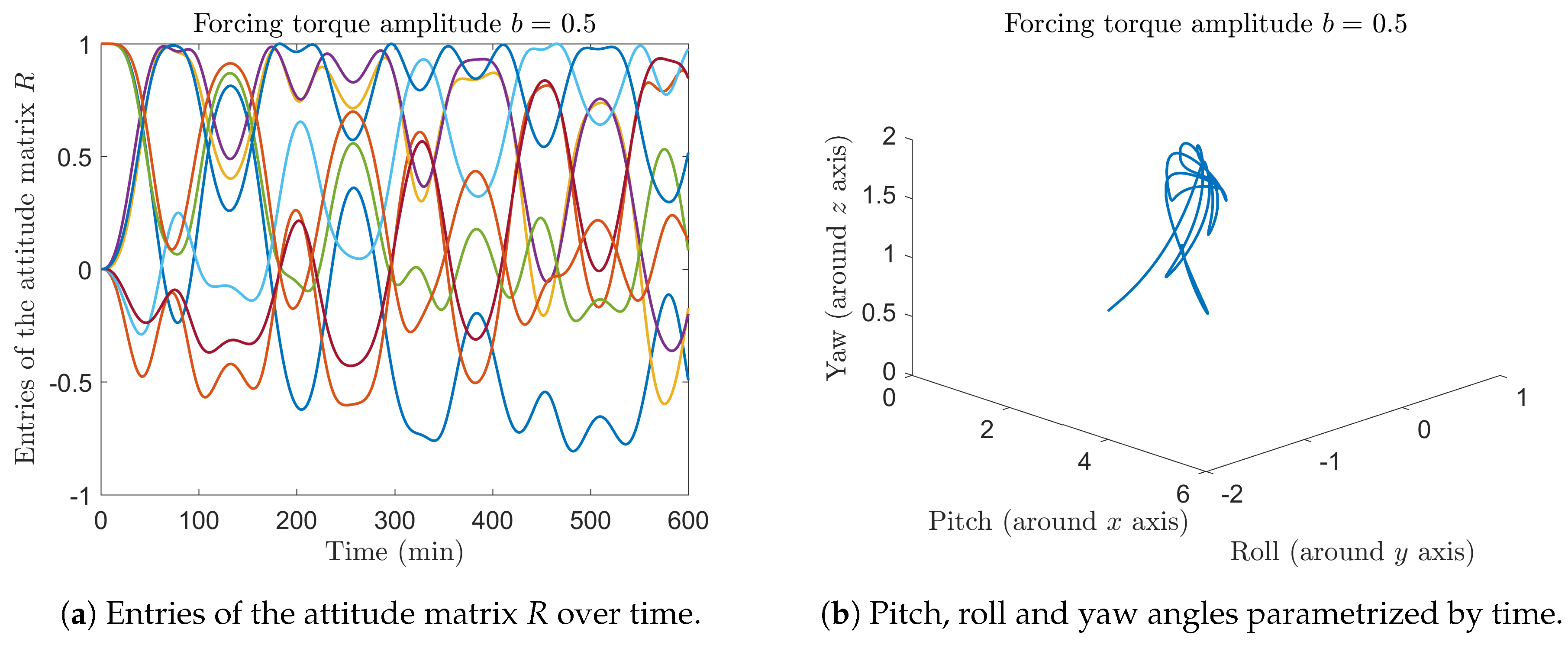
5.1. Numerical Integration of A Gyrostat Satellite Equations on $\mathrm{SO}\left(3\right)\times \mathfrak{so}\left(3\right)$

Let us summarize the equations of a gyrostat satellite, from the Section 3.1.5, as

$$\left\{\begin{array}{c}\phi :=[{\kappa }_1({\omega }_r-{\omega }_x)+{\kappa }_2({\omega }_r^3-{\omega }_x^3)]{\xi }_x+[{\kappa }_3({\omega }_r-{\omega }_y)+{\kappa }_4({\omega }_r^3-{\omega }_y^3)]{\xi }_y+[{\kappa }_5({\omega }_r-{\omega }_z)+{\kappa }_6({\omega }_r^3-{\omega }_z^3)]{\xi }_z,\hfill \\ D:=\mathrm{diag}\left(\sqrt{{\displaystyle \frac{J_y{J}_z}{J_x}}},\sqrt{{\displaystyle \frac{J_x{J}_z}{J_y}}},\sqrt{{\displaystyle \frac{J_x{J}_y}{J_z}}}\right),{\widehat{J}}_{\mathrm{g}}={\displaystyle \frac{1}{2}}\left[\begin{array}{ccc}{J}_y-J_x+J_z& 0& 0\\ 0& J_x-J_y+J_z& 0\\ 0& 0& J_x+J_y-J_z\end{array}\right],\hfill \\ {\xi }_1:=\left[\begin{array}{ccc}0& 0& 0\\ 0& 0& -{\omega }_1\\ 0& {\omega }_1& 0\end{array}\right],{\xi }_2:=\left[\begin{array}{ccc}0& 0& {\omega }_2\\ 0& 0& 0\\ -{\omega }_2& 0& 0\end{array}\right],{\xi }_3:=\left[\begin{array}{ccc}0& -{\omega }_3(1+bcos\left(\nu t\right))& 0\\ {\omega }_3(1+bcos\left(\nu t\right))& 0& 0\\ 0& 0& 0\end{array}\right],\hfill \\ \beta :=J_{11}{\xi }_1+J_{22}{\xi }_2+J_{33}{\xi }_3,\hfill \\ \dot{\xi }={\sigma }_{\xi }(\xi ,t), \mathrm{w}\mathrm{i}\mathrm{t}\mathrm{h} {\sigma }_{\xi }(\xi ,t):=D^{-1}\left([{\widehat{J}}_{\mathrm{g}},{\xi }^2]+[\beta ,\xi ]-\dot{\beta }-\{P,\xi \}+\phi \right)D^{-1},\hfill \\ \dot{R}={\sigma }_R(R,\xi ), \mathrm{w}\mathrm{i}\mathrm{t}\mathrm{h} {\sigma }_R(R,\xi ):=R\xi .\hfill \end{array}\right.$$

(119)

In the following numerical experiments, we take $t\in [0,600]$ (min) and initial conditions $\xi \left(0\right)=0$ and $R\left(0\right)=I_3$.

The differential equation $\dot{\xi }={\sigma }_{\xi }(\xi ,t)$ has support in $\mathfrak{so}\left(3\right)$, which is a vector space isomorphic to ${\mathbb{R}}^3$, hence it may be solved numerically by one of the numerical schemes outlined in the Section 4.1. The differential equation $\dot{R}={\sigma }_R(R,\xi )$ has support in $\mathrm{SO}\left(3\right)$, which is a curved space, hence it needs to be solved numerically by one of the numerical schemes outlined in the Section 4.2.

The numerical values of the parameters are taken from [7], namely:

$$\left\{\begin{array}{c}{J}_x=J_y=500,J_z=1000,\hfill \\ J_{11}{\omega }_1=J_{22}{\omega }_2=200,J_{33}{\omega }_3=250,\hfill \\ \gamma =200,\nu =\frac{1}{20},{\omega }_r=0,\hfill \end{array}\right.$$

(120)

where measurement units have been omitted. The amplitude b of the forcing oscillatory torque along the z axis varies. Moreover, the values of the controller constants ${\kappa }_1=\dots ={\kappa }_6$ may be varied to emphasize or de-emphasize the role of the attitude stabilizer.

We chose to employ an explicit Runge–Kutta method on manifold to solve Equation (119). The complete set of equations to simulate the motion of a gyrostat satellite read:

$$\left\{\begin{array}{c}{\xi }_{1,k}={\sigma }_{\xi }({\xi }_k,kT),{\xi }_{k+1/4}={\xi }_k+\frac{T}{2}{\xi }_{1,k},\hfill \\ {\xi }_{2,k}={\sigma }_{\xi }({\xi }_{k+1/4},kT+\frac{T}{2}),{\xi }_{k+1/2}={\xi }_k+\frac{T}{2}{\xi }_{2,k},\hfill \\ {\xi }_{3,k}={\sigma }_{\xi }({\xi }_{k+1/2},kT+\frac{T}{2}),{\xi }_{k+3/4}={\xi }_k+T{\xi }_{3,k},\hfill \\ {\xi }_{4,k}={\sigma }_{\xi }({\xi }_{k+3/4},kT+T),\hfill \\ {\xi }_{k+1}={\xi }_k+T(\frac{1}{6}{\xi }_{1,k}+\frac{1}{3}({\xi }_{2,k}+{\xi }_{3,k})+\frac{1}{6}{\xi }_{4,k}\hfill \\ {\xi }_{5,k}=T{R}_k{\xi }_k,R_{k+1/4}={\mathrm{Ret}}_{R_k}\left(\frac{1}{2}{\xi }_{5,k}\right),\hfill \\ {\xi }_{6,k}=T{R}_{k+1/4}{\xi }_{k+1/4},{\tilde{\xi }}_{6,k}={\mathrm{Par}}_{R_k}^{R_{k+1/4}}\left({\xi }_{6,k}\right),R_{k+1/2}={\mathrm{Ret}}_{R_k}\left(\frac{1}{2}{\tilde{\xi }}_{6,k}\right),\hfill \\ {\xi }_{7,k}=T{R}_{k+1/2}{\xi }_{k+1/2},{\tilde{\xi }}_{7,k}={\mathrm{Par}}_{R_k}^{R_{k+1/2}}\left({\xi }_{7,k}\right),R_{k+3/4}={\mathrm{Ret}}_{R_k}\left(\frac{1}{2}{\tilde{\xi }}_{7,k}\right),\hfill \\ {\xi }_{8,k}=T{R}_{k+3/4}{\xi }_{k+3/4},{\tilde{\xi }}_{8,k}={\mathrm{Par}}_{R_k}^{R_{k+3/4}}\left({\xi }_{8,k}\right),\hfill \\ R_{k+1}={\mathrm{Ret}}_{R_k}(\frac{1}{6}{\xi }_{5,k}+\frac{1}{3}({\tilde{\xi }}_{6,k}+{\tilde{\xi }}_{7,k})+\frac{1}{6}{\tilde{\xi }}_{8,k}).\hfill \end{array}\right.$$

(121)

where $k=0,1,2,\dots ,K$, ${\xi }_0=0$ and $R_0=I_3$. The first five equations represent an eRK4 method to advance the solution about the angular velocity matrix $\xi$, while the following five equations represent an eRK4M method to advance the solution about the attitude variable R. It is worth noticing that the intermediate values ${\xi }_{k+1/4}$, ${\xi }_{k+1/2}$ and ${\xi }_{k+3/4}$ calculated by the first three equations are reused in the seventh, eighth and ninth equations because the vector field ${\sigma }_R$ depends on $\xi$.

The Figure 4a,b show the results obtained by setting the forcing torque parameter b to $0.5$. Also, in this simulation we chose ${\kappa }_1=\dots ={\kappa }_6=1$. The Figure 4c,d show the results obtained when the forcing torque parameter b was set to $4.5$ and again ${\kappa }_1=\dots ={\kappa }_6=1$. In both experiments, it was set $T=0.01$ and K = 60,000, in such a way that the simulation spans 10 hours of motion. The trajectories look almost periodic, although perfect periodicity was never observed in the model-based numerical simulations. This particular result shows a slightly chaotic behavior in the motion of the modeled gyrostat satellite.

Figure 4. Entries of the attitude matrix R over time.

It is interesting to confirm numerically the role of the control torque $\phi$ in stabilizing the motion of the modeled gyrostat satellite. Figure 5 shows the results obtained by setting the forcing torque parameter b to $0.5$ and by zeroing the controller gains ${\kappa }_1=\dots ={\kappa }_6$. The simulated trajectory looks more chaotic compared to the previous case where the stabilizing control was switched on.

Figure 5. Entries of the attitude matrix R over time.

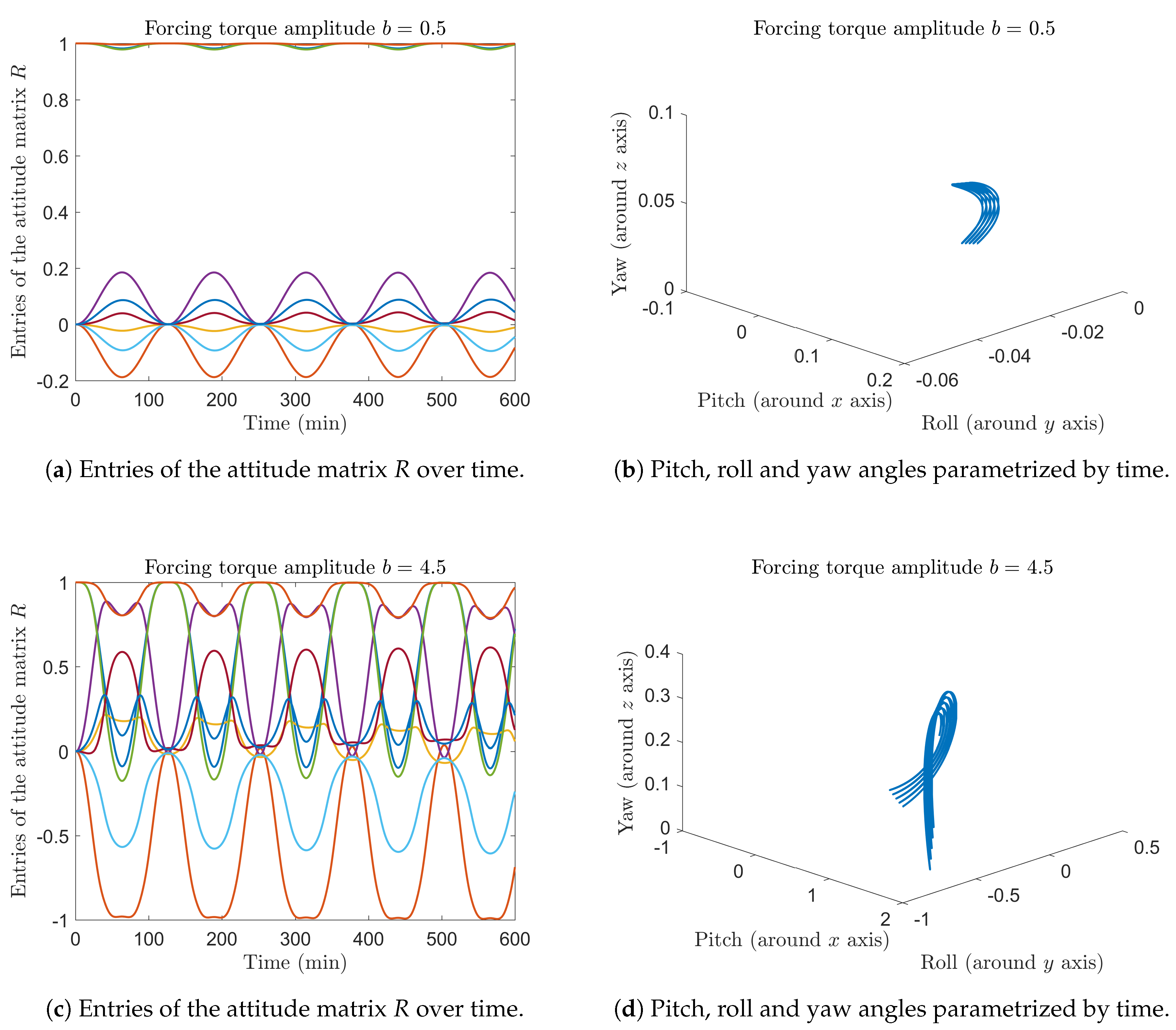
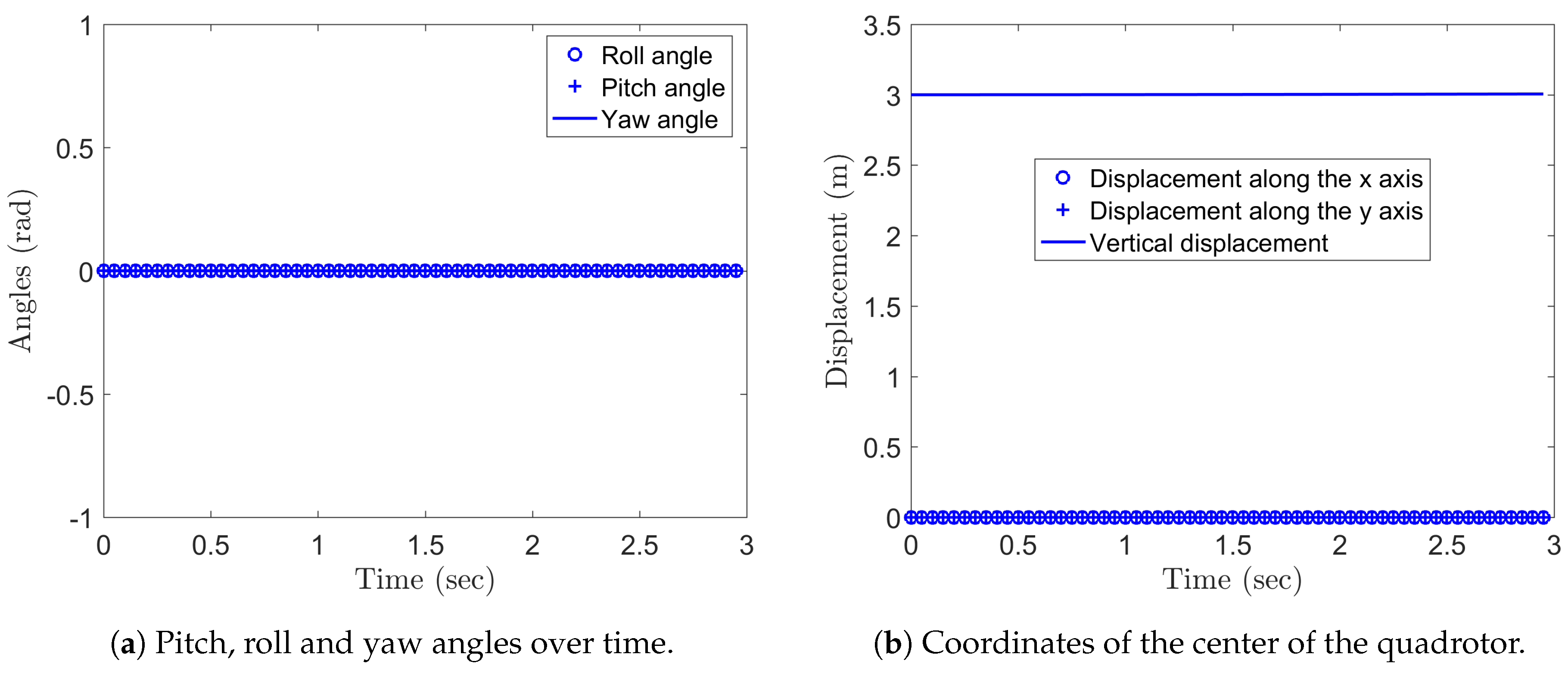
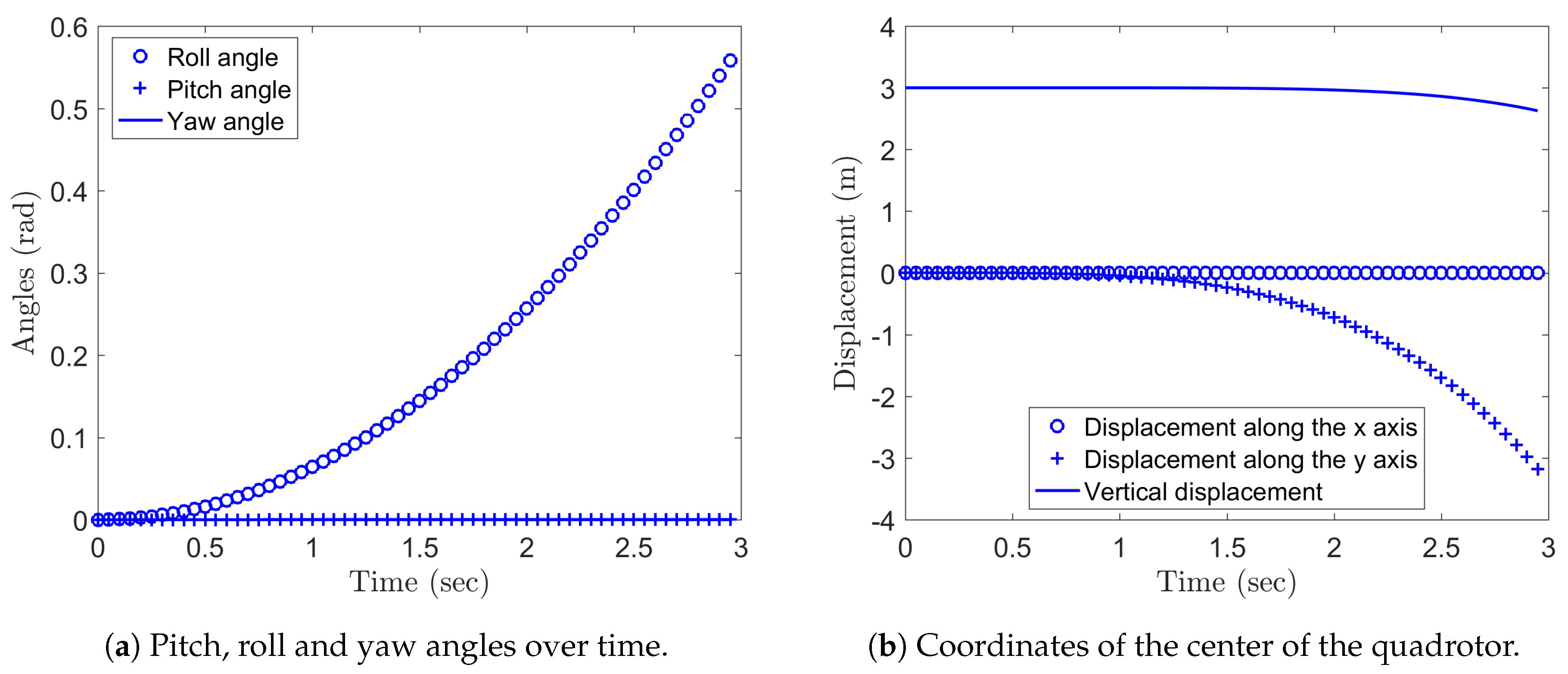
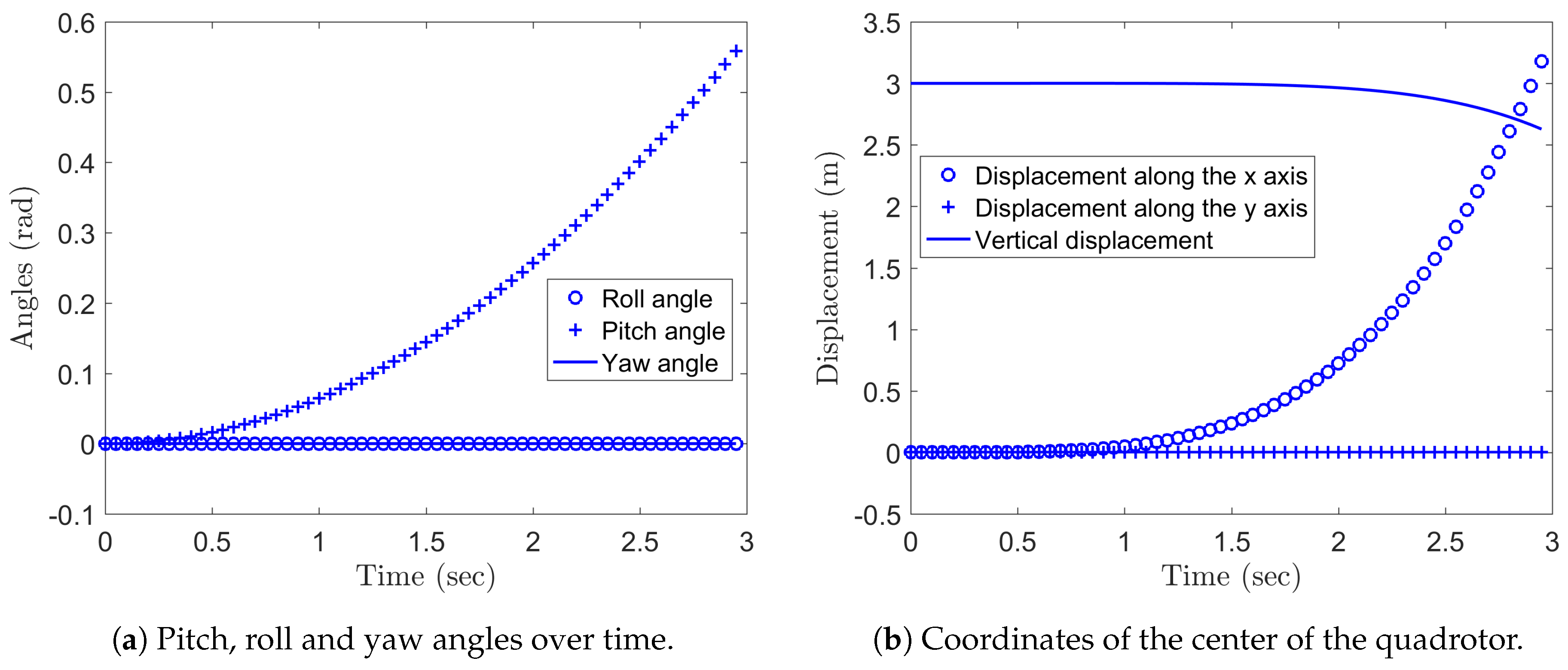
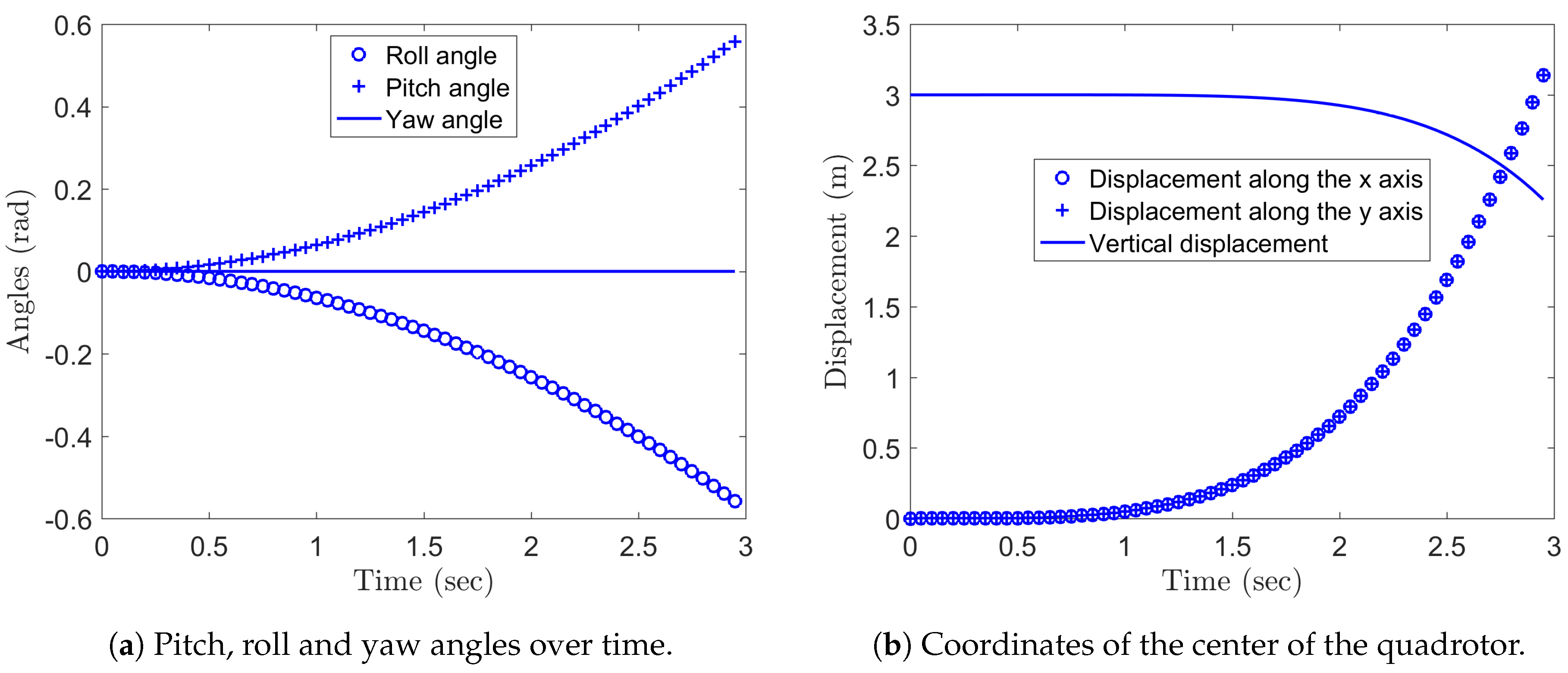
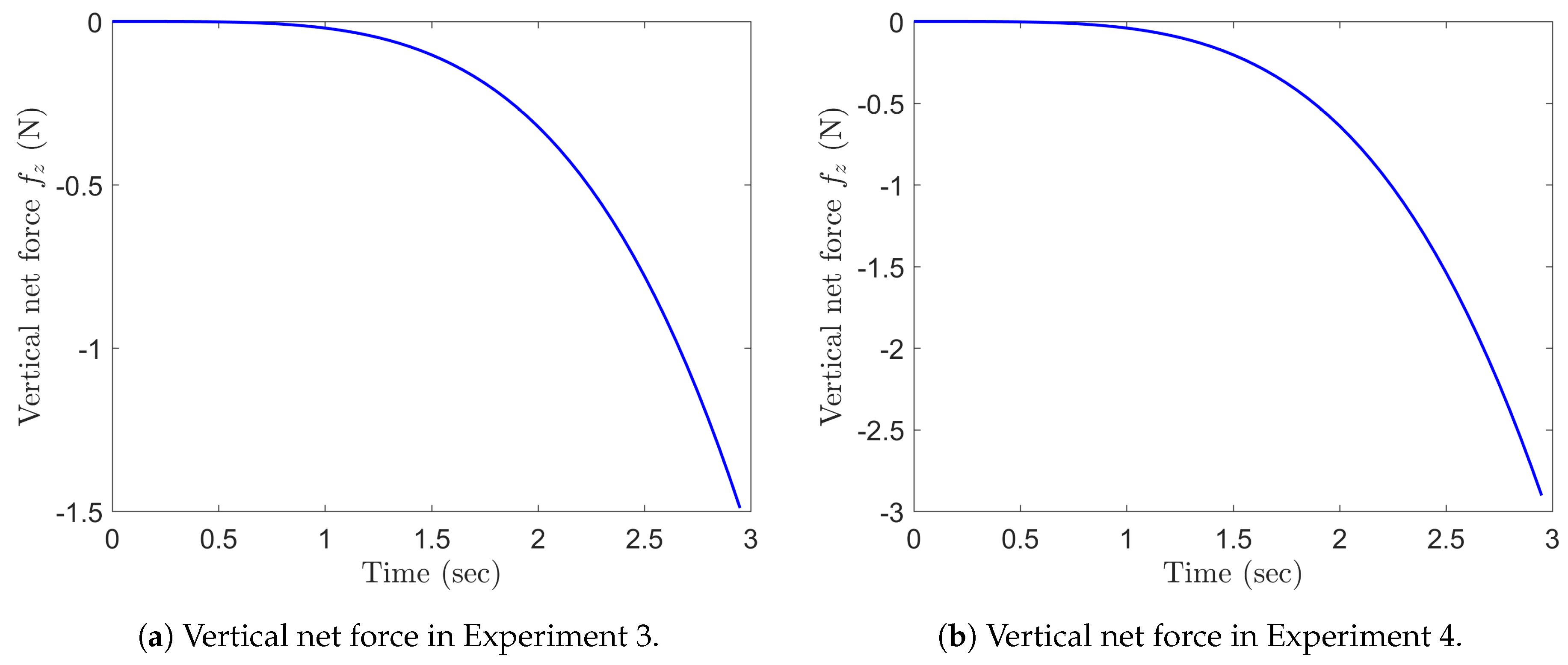
5.2. Integration of the Quadrotor Drone Equations on $\mathrm{SO}\left(3\right)\times \mathfrak{so}\left(3\right)\times {\mathbb{R}}^3$

Quadcopter modeling and simulation is a difficult and challenging problem. With six degrees of freedom (three translational and three rotational) and only four independent inputs (rotor speeds), quadcopters are severely underactuated. In order to achieve six degrees of freedom, rotational and translational motion are coupled, which result in coupled differential equations. Unlike ground vehicles, copters have very little friction to prevent their motion, so they must provide their own damping in order to stop moving and remain stable.

In order to implement a numerical simulation of the dynamics of a quadcopter, we recall from the Section 3.2.4 that the model includes a number of physical constants, four input variables, namely the spinning velocities of the four rotors ${\omega }_a\left(t\right)>0$, $a=1,2,3,4$, two state variables, $\xi \left(t\right)\in \mathfrak{so}\left(3\right)$ and $v\left(t\right)\in {\mathbb{R}}^3$, and two output variables, $R\left(t\right)\in \mathrm{SO}\left(3\right)$ and $q\left(t\right)\in {\mathbb{R}}^3$. Let us summarize the equations of a quadrotor drone from the Section 3.2.2 (equations for the rotational component of motions) and Section 3.2.3 (equations for the translational component of motion) as

$$\left\{\begin{array}{c}\tau :=br({\omega }_4^2-{\omega }_2^2){\xi }_x+br({\omega }_3^2-{\omega }_1^2){\xi }_y+\gamma (-{\omega }_1^2+{\omega }_2^2-{\omega }_3^2+{\omega }_4^2){\xi }_z,\hfill \\ {\mathsf{\Omega }}_r:=-{\omega }_1+{\omega }_2-{\omega }_3+{\omega }_4,\hfill \\ \beta :=J_{\mathcal{R}}{\mathsf{\Omega }}_r{\xi }_z,\hfill \\ D:=\mathrm{diag}\left(\sqrt{{\displaystyle \frac{J_y{J}_z}{J_x}}},\sqrt{{\displaystyle \frac{J_x{J}_z}{J_y}}},\sqrt{{\displaystyle \frac{J_x{J}_y}{J_z}}}\right),\hfill \\ {\widehat{J}}_{\mathrm{q}}={\displaystyle \frac{1}{2}}\left[\begin{array}{ccc}{J}_y-J_x+J_z& 0& 0\\ 0& J_x-J_y+J_z& 0\\ 0& 0& J_x+J_y-J_z\end{array}\right],\hfill \\ \dot{\xi }={\sigma }_{\xi }(\xi ,t),\mathrm{with}{\sigma }_{\xi }(\xi ,t):=D^{-1}([{\widehat{J}}_{\mathrm{q}},{\xi }^2]+[\beta ,\xi ]-\dot{\beta }+\tau )D^{-1},\hfill \\ \dot{R}={\sigma }_R(\xi ,t),\mathrm{with}{\sigma }_R(R,\xi ):=R\xi ,\hfill \\ \dot{v}={\sigma }_v(v,R,t),\mathrm{with}{\sigma }_v(v,R,t):=\frac{1}{2}\frac{b}{M_{\mathrm{q}}}({\omega }_1^2+{\omega }_2^2+{\omega }_3^2+{\omega }_4^2)R{\mathrm{e}}_z-p{\mathrm{e}}_z-\frac{1}{M_{\mathrm{q}}}\mathsf{\Gamma }v,\hfill \\ \dot{q}={\sigma }_q\left(v\right),\mathrm{with}{\sigma }_q\left(v\right):=v,\hfill \end{array}\right.$$

(122)

for $t\in [0,3]$ (sec). In order to simplify the numerical simulation, we will assume zero residual rotor angular velocity, namely ${\mathsf{\Omega }}_r=0$, in such a way that $\beta =0$ and $\dot{\beta }=0$. Therefore, the state transition function ${\sigma }_{\xi }$ simplifies to $D^{-1}([{\widehat{J}}_{\mathrm{q}},{\xi }^2]+\tau )D^{-1}$. The parameter $J_{\mathcal{R}}$ then disappears from the equations.

This differential system contains three equations on vector spaces (the equation for $\xi$ has support $\mathfrak{so}\left(3\right)$ and the equations for q and v have support ${\mathbb{R}}^3$) and an equation on manifold (the equation for R has support $\mathrm{SO}\left(3\right)$). The numerical values of the parameters are taken from [22], namely:

$$\left\{\begin{array}{c}{M}_{\mathrm{q}}=0.650,\hfill \\ J_x=J_y=7.5\times {10}^{-3},J_z=1.3\times {10}^{-2},\hfill \\ b=3.13\times {10}^{-5},r=0.23,\hfill \\ \gamma =7.5\times {10}^{-7},\hfill \\ p=9.81.\hfill \end{array}\right.$$

(123)

where measurement units are in the International System and have been omitted. We will also consider an isotropic aerodynamic drag, namely $\mathsf{\Gamma }=\frac{1}{4}{I}_3$. Several other aerodynamic effects could be included in the model as, for example, dependence of thrust on angle of attack, blade flapping and airflow disruption [44]. Since some of the aerodynamic effects have significant impact only at high velocities, these were excluded from the present model.

Even though the mathematical model deals with angular velocities ${\omega }_a$ as input variables, the input values are chosen to be the RPM $n_a$ of the rotors, because this is the more natural way of setting the propeller rotation velocity. The relation between angular velocity and rotation per minute is ${\omega }_a=\frac{\pi }{30}{n}_a$. We repeated the four test experiments suggested in ([20], Table 1) adapted to the present model. The rotors speed was adapted to the present case by means of a steady state design. Namely, we considered the case that the thrust produced by four rotors spinning at equal speed ${\omega }_{\mathrm{ss}}$ balances perfectly the gravitational force, formally:

$$\frac{1}{2}\frac{b}{M_{\mathrm{q}}}\left(4{\omega }_{\mathrm{ss}}^2\right)=p\Rightarrow {\omega }_{\mathrm{ss}}^2:=\frac{p{M}_{\mathrm{q}}}{2b}.$$

(124)

The resulting steady-state rotor speed in RPM (rounded to the nearest integer) reads

$$n_{\mathrm{ss}}:=⌊\frac{30}{\pi }\sqrt{\frac{g{M}_{\mathrm{q}}}{2b}}⌋=3048.$$

(125)

When the quadcopter is tilted, namely $R\ne I_3$, the total thrust only approximately balances the gravitational acceleration, hence the quadcopter is subjected to a vertical lift. Moreover, upon tilting, the quadcopter might be subjected to a horizontal force, whose combined effect with the vertical lift causes its change of direction. An estimation of the net force, in the earth frame, under a common operation condition, is outlined in the following

Lemma 6.

Define the net force acting on the quadcopter’s center of mass as

$$f_{\mathrm{net}}:=\frac{1}{2}\frac{b}{M_{\mathrm{q}}}\left(\sum _{a=1}^4{\omega }_a^2\right)R{\mathrm{e}}_z-p{\mathrm{e}}_z.$$

(126)

Assume that${\omega }_a={\omega }_{\mathrm{ss}}+\mathsf{\Delta }{\omega }_a$, with${\sum }_a{(-1)}^a\mathsf{\Delta }{\omega }_a=0$and${\sum }_a\mathsf{\Delta }{\omega }_a=0$. In addition, assume that${\left(\mathsf{\Delta }{\omega }_1\right)}^2+{\left(\mathsf{\Delta }{\omega }_2\right)}^2\ll 2{\omega }_{\mathrm{ss}}^2$. Then it follows that, to first order,

$$f_{\mathrm{net}}\approx p(R-I_3){\mathrm{e}}_z.$$

(127)

Proof. 

By the binomial theorem, we get ${\omega }_a^2={\omega }_{\mathrm{ss}}^2+{\left(\mathsf{\Delta }{\omega }_a\right)}^2+2{\omega }_{\mathrm{ss}}\mathsf{\Delta }{\omega }_a$. Summing over the index a we then get

$$\sum _a{\omega }_a^2=4{\omega }_{\mathrm{ss}}^2+\sum _a{\left(\mathsf{\Delta }{\omega }_a\right)}^2+2{\omega }_{\mathrm{ss}}\sum _a\mathsf{\Delta }{\omega }_a.$$

(128)

From the conditions ${\sum }_a{(-1)}^a\mathsf{\Delta }{\omega }_a=0$ and ${\sum }_a\mathsf{\Delta }{\omega }_a=0$ it follows that $\mathsf{\Delta }{\omega }_4=-\mathsf{\Delta }{\omega }_2$ and $\mathsf{\Delta }{\omega }_3=-\mathsf{\Delta }{\omega }_1$, therefore ${\sum }_a{\left(\mathsf{\Delta }{\omega }_a\right)}^2=2({\left(\mathsf{\Delta }{\omega }_1\right)}^2+{\left(\mathsf{\Delta }{\omega }_2\right)}^2)$ and thus

$$\sum _a{\omega }_a^2=4{\omega }_{\mathrm{ss}}^2+2({\left(\mathsf{\Delta }{\omega }_1\right)}^2+{\left(\mathsf{\Delta }{\omega }_2\right)}^2).$$

(129)

$$f_{\mathrm{net}}=\frac{b}{M_{\mathrm{q}}}(2{\omega }_{\mathrm{ss}}^2+{\left(\mathsf{\Delta }{\omega }_1\right)}^2+{\left(\mathsf{\Delta }{\omega }_2\right)}^2)R{\mathrm{e}}_z-p{\mathrm{e}}_z.$$

(130)

By way of the assumption that ${\left(\mathsf{\Delta }{\omega }_1\right)}^2+{\left(\mathsf{\Delta }{\omega }_2\right)}^2\ll 2{\omega }_{\mathrm{ss}}^2$, we can neglect the second and third addendum in the parentheses of the relation (130) and write

$$f_{\mathrm{net}}\approx \frac{2b}{M_{\mathrm{q}}}{\omega }_{\mathrm{ss}}^{2}R{\mathrm{e}}_z-p{\mathrm{e}}_z.$$

(131)

From the definition (124) it follows the assertion. □

The condition ${\sum }_a{(-1)}^a\mathsf{\Delta }{\omega }_a=0$ ensures that the residual ${\mathsf{\Omega }}_r$ stays null. The hypothesis that ${\sum }_a\mathsf{\Delta }{\omega }_a=0$ is a key assumption to simplify the analysis (and to design a controller). The assumption ${\left(\mathsf{\Delta }{\omega }_1\right)}^2+{\left(\mathsf{\Delta }{\omega }_2\right)}^2\ll 2{\omega }_{\mathrm{ss}}^2$ reflects the fact that, to produce a manageable unbalance in the thrusts, the RPM of the rotors need to change just slightly. Not surprisingly, the net force $f_{\mathrm{net}}$ is proportional to the tilt $R-I_3$. The vertical lift, that causes a quadcopter to change its altitude, is

$$f_z:={\mathrm{e}}_z^{\top }{f}_{\mathrm{net}}\approx p({\mathrm{e}}_z^{\top }R{\mathrm{e}}_z-1),$$

(132)

estimated by default.

It is also important to estimate the yaw effect due to rotors drag under the same conditions of the Lemma 6. An exact estimation is outlined in the following

Lemma 7.

Define the mechanical torque responsible for the yaw of the drone as in (90) as

$${\tau }_z:=\gamma \sum _{a=1}^4{(-1)}^a{\omega }_a^2.$$

(133)

Under the same hypotheses of Lemma 6, it holds that

$${\tau }_z=2\gamma ({\left(\mathsf{\Delta }{\omega }_2\right)}^2-{\left(\mathsf{\Delta }{\omega }_1\right)}^2).$$

(134)

Proof. 

By the binomial theorem, we get

$$\sum _a{(-1)}^a{\omega }_a^2={\omega }_{\mathrm{ss}}^2\sum _a{(-1)}^a+\sum _a{(-1)}^a{\left(\mathsf{\Delta }{\omega }_a\right)}^2+2{\omega }_{\mathrm{ss}}\sum _a{(-1)}^a\mathsf{\Delta }{\omega }_a.$$

(135)

The first term on the right-hand side is null. From the conditions ${\sum }_a{(-1)}^a\mathsf{\Delta }{\omega }_a=0$ and ${\sum }_a\mathsf{\Delta }{\omega }_a=0$, it follows that the third term on the right-hand side is null and that ${\left(\mathsf{\Delta }{\omega }_4\right)}^2={\left(\mathsf{\Delta }{\omega }_2\right)}^2$ and ${\left(\mathsf{\Delta }{\omega }_3\right)}^2={\left(\mathsf{\Delta }{\omega }_1\right)}^2$. Therefore, ${\sum }_a{(-1)}^a{\left(\mathsf{\Delta }{\omega }_a\right)}^2=2({\left(\mathsf{\Delta }{\omega }_2\right)}^2-{\left(\mathsf{\Delta }{\omega }_1\right)}^2)$ and thus the assertion. □

The rotors RPM used in the experiments, adapted from [20], are outlined in Table 1. Notice that, in all four experiments, the residual angular velocity is null, namely ${\mathsf{\Omega }}_r=0$, and that the angular deviations $\mathsf{\Delta }{\omega }_a$ satisfy all the assumptions made in the Lemma 6. Furthermore, since all $|\mathsf{\Delta }{\omega }_a|$ are either 0 or $\frac{\pi }{30}$, and since the drag constant γ is really small in this quadcopter model, according to Lemma 7, we expect the yaw component of the external torque ${\tau }_z$ to be practically negligible in all four numerical experiments.

Table 1. Summary of four numerical experiments’ design.

Experiment	Rotors RPM
	${\mathit{n}}_{\mathbf{1}}$	${\mathit{n}}_{\mathbf{2}}$	${\mathit{n}}_{\mathbf{3}}$	${\mathit{n}}_{\mathbf{4}}$
First	3048	3048	3048	3048
Second	3048	3047	3048	3049
Third	3047	3048	3049	3048
Fourth	3047	3049	3049	3047

We chose to integrate the differential equations that describe the rotational component of motion as well as the translational component of motion by means of a forward Euler scheme. The complete set of equations read:

$$\left\{\begin{array}{c}{\xi }_{k+1}={\xi }_k+T{\sigma }_{\xi }({\xi }_k,kT),\hfill \\ R_{k+1}={\mathrm{Ret}}_{R_k}\left(T{R}_k{\xi }_k\right),\hfill \\ v_{k+1}=v_k+T{\sigma }_v(v_k,R_k,kT),\hfill \\ q_{k+1}=q_k+T{\sigma }_q\left(v_k\right),\hfill \end{array}\right.$$

(136)

where $k=0,1,2,\dots ,K$, ${\xi }_0=0$, $R_0=I_3$, $q_0=3{\mathrm{e}}_z$ and $v_0=0$. In all the following four experiments, it was chosen $K=3000$ and $T=0.001$ (the experiments will predict the first 3 seconds of dynamics).

In Experiment 1, the rotors RPM is fixed to $n_{\mathrm{ss}}$. In this experiment, the thrusts are perfectly balanced, hence the quadcopter is supposed to maintain the initial position and the initial attitude over time, that means no pitching, rolling nor yawing, nor vertical displacement. The Figure 6 show the results obtained by the numerical scheme (136), which confirm the intuitive prediction.

Figure 6. Pitch, roll and yaw angles over time.

In the Experiment 2, $n_1=n_3=n_{\mathrm{ss}}$, while $n_2=n_{\mathrm{ss}}-1$ and $n_4=n_{\mathrm{ss}}+1$. The unbalance in the rotation speed of the rotors ${\mathcal{R}}_2$ and ${\mathcal{R}}_4$ causes the quadcopter to rotate along the z axis (to yaw) and to tilt along the x axis (to roll) which, in turn, causes the quadrotor to move along the y axis. Since $n_4>n_2$, the rotor ${\mathcal{R}}_4$ pulls stronger than the rotor ${\mathcal{R}}_2$, hence the drone actually shifts in the $-y$ direction. The Figure 7 show the results obtained by the numerical scheme (136). Notice that the model (122) does not include any controller, therefore the slight unbalance in the propellers RPM causes an unbalance between the thrust and the gravitational attraction which, in turn, causes a drop in the quadcopter altitude. (For an example of proportional-derivative controller employed in quadcopter maneuvering, see [45].) As it was predicted by way of Lemma 7, the yaw is negligible.

Figure 7. Pitch, roll and yaw angles over time.

In the Experiment 3, $n_2=n_4=n_{\mathrm{ss}}$, while $n_1=n_{\mathrm{ss}}-1$ and $n_3=n_{\mathrm{ss}}+1$. The unbalance in the rotation speed of the rotors ${\mathcal{R}}_1$ and ${\mathcal{R}}_3$ causes the quadcopter to yaw and to tilt along the y direction (that is, to pitch). The tilting causes the center of the quadrotor drone to shift along the x axis. The Figure 8 show the results obtained by the numerical scheme (136). Since $n_3>n_1$, the rotor ${\mathcal{R}}_3$ pulls stronger than the rotor ${\mathcal{R}}_1$, hence (readers might want to refer to Figure 3) the drone actually shifts in the $+x$ direction. Again notice that, because the model (122) does not include any feedback controller, the slight unbalance in the propellers RPM causes a drop in the quadcopter altitude, while, again, the yaw effect results to be negligible.

Figure 8. Pitch, roll and yaw angles over time.

In the Experiment 4, $n_2=n_3=n_{\mathrm{ss}}+1$, while $n_1=n_4=n_{\mathrm{ss}}-1$. The unbalance in the rotation speed of the rotors ${\mathcal{R}}_1$ and ${\mathcal{R}}_3$ causes the quadcopter to pitch and to shift toward the $+x$ direction and, at the same time, the unbalance in the rotation speed of the rotors ${\mathcal{R}}_2$ and ${\mathcal{R}}_4$ causes the quadcopter to roll and to shift toward the $+y$ direction. Due to the assumed perfect symmetry of the model, equal unbalance in the propellers rotation speed results in equal shifting along both x and y axes. The Figure 9 show the results obtained by the numerical scheme (136), which confirm the intuition. Because of the combined action of all propellers, in this case no drop in the quadcopter altitude nor yawing of the quactopter body are predicted by the model.

Figure 9. Pitch, roll and yaw angles over time.

Through the numerical scheme, we can compare the values of the vertical net force predicted by the model through the relation (132) in two experiments, for example in Experiment 3 and Experiment 4. The Figure 10 show the results of this comparison. The force $f_z$ in Experiment 4 almost doubles the force predicted in Experiment 3, which explains the larger predicted drop in the altitude of the quadcopter in the Figure 9.

Figure 10. Vertical net force in Experiment 3.

6. Conclusions

A large number of scientific problems are most naturally described by systems of first-order differential and algebraic equations. Numerical methods for solving initial value problems are extremely important, because analytic solutions exist only in very special cases (e.g., for linear equations, exact equations, non-exact equations with integrating factors, and equations that are homogeneous of degree 0). Any first-order initial value problem can be solved (or “integrated”) numerically by discretizing the interval of integration into a number of sub-intervals, either with equally or non-equally distributed grid points. As the integration advances, the numerical solutions at the grid points are approximated.

In the recent years, it has come to the attention of researchers in applied sciences and engineering how classical numerical methods, designed to solve initial value problems on ${\mathbb{R}}^n$ are unsuitable to solve differential equations formulated on differentiable manifolds. These differential equations represent compactly large systems of mixed non-linear differential/algebraic equations, where the algebraic sub-equations carry on mutual constraints among the variables.

In the present paper, we recalled the formulation of non-conservative system dynamics through the Lagrange–d’Alembert principle and the generalized Euler–Poincaré form of the system equation on Lie groups. The Euler–Poincaré equations for left-invariant Lagrangians were illustrated via derivation of the dynamical equations for a gyrostat satellite and for a quadcopter drone.

Numerical experiments carried out by way of a forward Euler method on a manifold and an explicit fourth-order Runge–Kutta method on manifold illustrated the numerical integration of the Euler–Poincaré equations on the special orthogonal group $\mathrm{SO}\left(3\right)$. A number of questions are still an open problem and will be the focus of future investigation:

• The problem about the order of the numerical schemes, which may be studied either analytically and by means of numerical experiments. The present author has started an analysis of the order of some numerical schemes which rely on ad-hoc Taylor-series-like expansions [46]. It would also be informative to use examples for which the analytic solution is known, and then compare the two numerical solutions to the analytic solution individually. This would also allow for the error order of the Runge–Kutta method to be evaluated numerically. While it is true that closed-form solutions of ODEs on nonlinear spaces cannot be obtained in general, the solutions are available in special cases, as shown in [47].
• The problem of the convergence of the numerical schemes, which is quite involved, being the algorithms considered in this paper of complex non-linear nature. The numerical schemes were stable in the numerical simulations performed in the course of this study. In general, it is expected that they would enjoy/suffer from the same advantages/drawbacks of their precursors.
• An accurate evaluation of the computational complexity of the forward Euler method and of the Runge–Kutta integration method.
• It would be very interesting to design more model-based experimental settings to survey the behavior of the studied satellite gyrostat. For example, it would be interesting to study a control strategy to see if it is possible to set the inputs ${\omega }_1,{\omega }_2,{\omega }_3$ so as to make the satellite gain a prescribed attitude with respect to the earth-fixed reference frame. On the same line, it would be interesting to enrich the model (119) with a (possibly differential) equation that describes the relationship between the motors control voltages and the rotors rotation speed, in order to make the control scheme more realistic.

References

- Arnol’d, V.I. Mathematical Methods of Classical Mechanics; Springer: New York, NY, USA, 1989; (Originally published by Nauka, Moscow, 1974. Translated by A. Weinstein and K. Vogtmann). [Google Scholar]
- Abraham, R.; Marsden, J.E.; Ratiu, T.S. Manifolds, Tensor Analysis, and Applications; Springer: New York, NY, USA, 1988; (Originally published by Addison-Wesley Publishing Company, 1983). [Google Scholar]
- Bullo, F.; Lewis, A.D. Geometric Control of Mechanical Systems: Modeling, Analysis, and Design for Mechanical Control Systems; Springer: New York, NY, USA, 2005. [Google Scholar]
- Fiori, S. Nonlinear damped oscillators on Riemannian manifolds: Fundamentals. J. Syst. Sci. Complex. 2016, 29, 22–40. [Google Scholar] [CrossRef]
- Fiori, S. Nonlinear damped oscillators on Riemannian manifolds: Numerical simulation. Commun. Nonlinear Sci. Numer. Simul. 2017, 47, 207–222. [Google Scholar] [CrossRef]
- Bloch, A.; Krishnaprasad, P.S.; Marsden, J.E.; Ratiu, T.S. The Euler–Poincaré equations and double bracket dissipation. Commun. Math. Phys. 1996, 175, 1–42. [Google Scholar] [CrossRef]
- Ge, Z.-M.; Lin, T.-N. Chaos, chaos control and synchronization of a gyrostat system. J. Sound Vib. 2002, 251, 519–542. [Google Scholar] [CrossRef]
- Marsden, J.E.; Ratiu, T.S. Introduction to Mechanics and Symmetry—A Basic Exposition of Classical Mechanical Systems, 2nd ed.; Texts in Applied Mathematics (Book 17); Springer: New York, NY, USA, 2002. [Google Scholar]
- Holm, D.D. Geometric Mechanics—Part I: Dynamics and Symmetry, 2nd rev. ed.; Imperial College Press: London, UK, 2011. [Google Scholar]
- Holm, D.D. Geometric Mechanics—Part II: Rotating, Translating And Rolling, 2nd ed.; Imperial College Press: London, UK, 2011. [Google Scholar]
- Aslanov, V. Behavior of a free dual-spin gyrostat with different ratios of inertia moments. Adv. Math. Phys. 2015, 2015, 323714. [Google Scholar] [CrossRef]
- Tong, C. Lord Kelvin’s gyrostat and its analogs in physics, including the Lorenz model. Am. J. Phys. 2009, 77, 526. [Google Scholar] [CrossRef]
- Hall, C.D. Momentum transfer in two-rotors gyrostat. J. Guid. Control. Dyn. 1996, 19, 1157–1161. [Google Scholar] [CrossRef]
- Yu, W.; Pan, Z. Dynamical equations of multibody systems on Lie groups. Adv. Mech. Eng. 2015, 7, 1–9. [Google Scholar] [CrossRef]
- Tong, X.; Tabarrok, B.; Rimrott, F.P.J. Chaotic motion of an asymmetric gyrostat in the gravitational field. Int. J. Non-Linear Mech. 1995, 30, 191–203. [Google Scholar] [CrossRef]
- Bezglasnyi, S. Stabilization of gyrostat motion with cavity filled with viscous fluid. In Proceedings of the World Congress on Engineering (WCE 2015), London, UK, 1–3 July 2015; Volume 1. [Google Scholar]
- Hamm, A.; Lin, Z. “Why drones for ordinary people?” Digital representations, topic clusters, and techno-nationalization of drones on Zhihu. Information 2019, 10, 256. [Google Scholar] [CrossRef]
- Moskalenko, V.; Moskalenko, A.; Korobov, A.; Semashko, V. The model and training algorithm of compact drone autonomous visual navigation system. Data 2019, 4, 4. [Google Scholar] [CrossRef]
- Lynskey, J.; Thar, K.; Oo, T.Z.; Hong, C.S. Facility location problem approach for distributed drones. Symmetry 2019, 11, 118. [Google Scholar] [CrossRef]
- Benić, Z.; Piljek, P.; Kotarski, D. Mathematical modelling of unmanned aerial vehicles with four rotors. Interdiscip. Descr. Complex Syst. 2016, 14, 88–100. [Google Scholar]
- Goodarzi, F.A.; Lee, D.; Lee, T. Geometric control of a quadrotor UAV transporting a payload connected via flexible cable. Int. J. Control. Autom. Syst. 2015, 13, 1486–1498. [Google Scholar] [CrossRef]
- Becker, M.; Sampaio, R.C.B.; Bouabdallah, S.; de Perrot, V.; Siegwart, R. In-flight collision avoidance controller based only on OS4 embedded sensors. J. Braz. Soc. Mech. Sci. Eng. 2012, 34, 294–307. [Google Scholar] [CrossRef]
- Lambert, J.D.; Lambert, D. Numerical Methods for Ordinary Differential Systems: The Initial Value Problem; Wiley: New York, NY, USA, 1991; Chapter 5. [Google Scholar]
- Hairer, E.; Lubich, C.; Wanner, G. Geometric Numerical Integration: Structure-Preserving Algorithms for Ordinary Differential Equations, 2nd ed.; Springer: Berlin, Germany; New York, NY, USA, 2006. [Google Scholar]
- Cear, C.W. Numerical Initial Value Problems in Ordinary Differential Equations; Prentice-Hall: Upper Saddle River, NJ, USA, 1973. [Google Scholar]
- Milne, W.E. Numerical integration of ordinary differential equations. Am. Math. Mon. 1926, 33, 455–460. [Google Scholar] [CrossRef]
- Euler, L. Institutionum Calculi Integralis. Volumen Secundum (1769); Kowalewski, G., Ed.; Opera Omnia Series 1; Opera Mathematica; 1914; Available online: http://sites.mathdoc.fr/cgi-bin/oeitem?id=OE_EULER_1_12_1_0 (accessed on 3 August 2019).
- Henrici, P. Discrete Variable Methods in Ordinary Differential Equations; Wiley: New York, NY, USA, 1962. [Google Scholar]
- Hairer, E.; Nørsett, S.P.; Wanner, G. Solving Ordinary Differential Equations, I. Nonstiff Problems; Springer: Berlin/Heidelberg, Germany, 1987. [Google Scholar]
- Lambert, J.D. Computational Methods In Ordinary Differential Equations; Wiley: London, UK, 1973. [Google Scholar]
- Dekker, K.; Verwer, J.G. Stability of Runge–Kutta Methods for Stiff Nonlinear Differential Equations; CWI Monographs, 2; North-Holland: Amsterdam, The Natherlands, 1984. [Google Scholar]
- Butcher, J.C. The Numerical Analysis of Ordinary Differential Equations. Runge–Kutta and General Linear Methods; Wiley-Interscience: New York, NY, USA, 1987. [Google Scholar]
- Stetter, H.J. Analysis of Discretization Methods for Ordinary Differential Equations; Springer: Berlin/Heidelberg, Germany, 1973. [Google Scholar]
- Obrechkoff, N. Neue Kwadraturformuln; Abh. Preuss. Akad. Wiss. Math.-Nat. Kl.: Berlin, Germany, 1940; Volume 4. [Google Scholar]
- Merson, R.H. An operational method for the study of integration processes. In Proceedings of the Symposium in Weapons Research Establishment, Salisbury, Australia, 3–8 June 1957; pp. 110–125. [Google Scholar]
- Stoer, J.; Bulirsch, R. Introduction to Numerical Analysis, 3rd ed.; Springer-Verlag: Berlin, Germany; New York, NY, USA, 2002. [Google Scholar]
- Fiori, S. Gyroscopic signal smoothness assessment by geometric jolt estimation. Math. Methods Appl. Sci. 2017, 40, 5893–5905. [Google Scholar] [CrossRef]
- Celledoni, E.; Fiori, S. Neural learning by geometric integration of reduced ‘rigid-body’ equations. J. Comput. Appl. Math. 2004, 172, 247–269. [Google Scholar] [CrossRef]
- Bobenko, A.I.; Suris, Y.B. Discrete time Lagrangian mechanics on Lie groups, with an application to the Lagrange top. Commun. Math. Phys. 1999, 204, 147–188. [Google Scholar] [CrossRef]
- Marsden, J.E.; Pekarsky, S.; Shkoller, S. Discrete Euler–Poincaré and Lie-Poisson equations. Nonlinearity 1999, 12, 1647–1662. [Google Scholar] [CrossRef]
- Marsden, J.E.; Pekarsky, S.; Shkoller, S. Symmetry reduction of discrete Lagrangian mechanics on Lie groups. J. Geom. Phys. 2000, 36, 140–151. [Google Scholar] [CrossRef]
- Bou-Rabee, N.; Marsden, J.E. Hamilton–Pontryagin Integrators on Lie Groups Part I: Introduction and Structure-Preserving Properties. Found. Comput. Math. 2009, 9, 197–219. [Google Scholar] [CrossRef]
- Kobilarov, M.; Crane, K.; Desbrun, M. Lie group integrators for animation and control of vehicles. ACM Trans. Graph. 2009, 28, 16. [Google Scholar] [CrossRef]
- Huang, H.; Hoffmann, G.M.; Waslander, S.L.; Tomlin, C.J. Aerodynamics and control of autonomous quadrotor helicopters in aggressive maneuvering. In Proceedings of the IEEE International Conference on Robotics and Automation, Kobe, Japan, 12–17 May 2009; pp. 3277–3282. [Google Scholar]
- Shahid, F.; Kadri, M.B.; Jumani, N.A.; Pirwani, Z. Dynamical modeling and control of quadrotor. Trans. Mach. Des. 2016, 4, 50–63. [Google Scholar]
- Fiori, S. A closed-form expression of the instantaneous rotational lurch index to evaluate its numerical approximation. Symmetry 2019, 11, 1208. [Google Scholar] [CrossRef]
- Markdahl, J.; Hu, X. Exact solutions to a class of feedback systems on SO(n). Automatica 2016, 63, 138–147. [Google Scholar] [CrossRef]
© 2019 by the author. Licensee MDPI, Basel, Switzerland. This article is an open access article distributed under the terms and conditions of the Creative Commons Attribution (CC BY) license (http://creativecommons.org/licenses/by/4.0/).