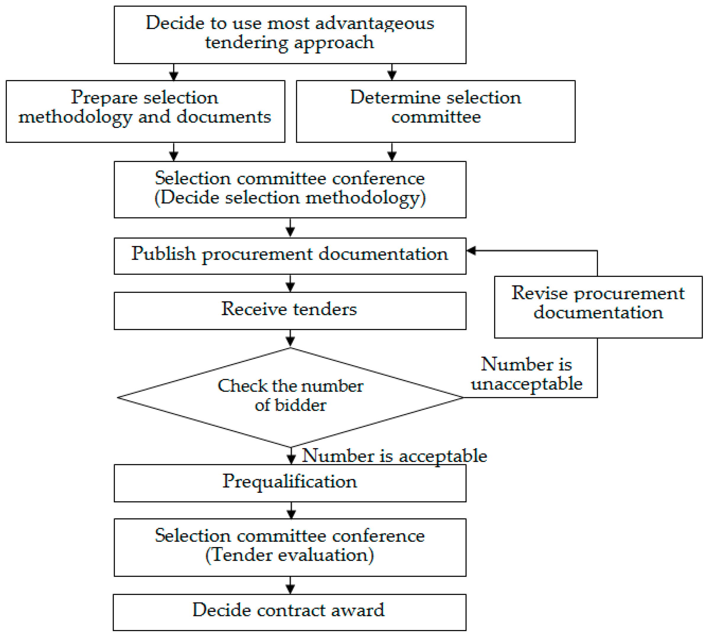
Article

Application of Optimization to Select Contractors to Develop Strategies and Policies for the Development of Transport Infrastructure

1
Department of Industrial Engineering and Management, National Kaohsiung University of Sciences and Technology, Chien Kung Campus, 415 Chien Kung Road, Kaohsiung 807, Taiwan
2
Department of Industrial Engineering and Management, Fortune Institute of Technology, Kaohsiung 83160, Taiwan
3
Faculty of Economics, Thu Dau Mot University, Number 6, Tran Van On Street, Phu Hoa Ward, Thu Dau Mot City 820000, Binh Duong Province, VietNam
*
Author to whom correspondence should be addressed.
Mathematics 2019, 7(1), 98; https://doi.org/10.3390/math7010098
Submission received: 9 December 2018 / Revised: 4 January 2019 / Accepted: 12 January 2019 / Published: 18 January 2019

Abstract

:
Many factors influence the efficiency and quality of transport works. In particular, consultants and construction contractors of these works play important roles, and critical factors directly affect the quality of traffic works. If the quality of consultancy and construction is good, the project will reduce the total investment; if the contractor is good, the completion time of the new project is guaranteed, thus reducing construction costs. The longer the construction time is, the higher the cost of the project. In this study, the authors used optimal algorithms to evaluate past, present, and future contractors’ technical, technological, and performance effectiveness. Research results show that bidders are divided into three groups: highly effective bidders, stable contractors, and inefficient groups. Research results for this subject will help the government, regulatory agencies, and investors select good contractors as the basis for developing strategies and policies for the development of transport infrastructure.

1. Introduction

Contractor Selection Procedure: There are currently many models for selecting contractors for transport infrastructure projects, in which the best bidder selection model by Jyh-Bin Yang and Wei-Chih Wang is utilized (Figure 1).
Choosing a contractor for construction of traffic works is an important issue. Therefore, the contractor must have sufficient professional capacity, human resources, and financial capacity. Depending on the scale, the nature and sources of capital for the construction of traffic works are considered when selecting contractors. In particular, the selection of contractors for transport works is divided into three main forms as follows [2]:
Open bidding: Used to select contractors for construction works in the form of unlimited number of participating contractors.
Restricted bidding: To be used for the selection of contractors for construction of transport works; there are only a number of contractors that meet all the conditions in regard to the capability of construction activities and the capability of practicing the construction of works. Traffic is invited to participate in bidding.
Appointment of contractor: Investment deciders or investors of transport works are entitled to designate contractors directly qualified for construction activities and are capable of practicing construction of traffic works at a reasonable cost.
Each traffic works in different areas require different qualifications, construction techniques, and experience. In order to ensure that construction works are designed to bring economic efficiency for the investor in particular and the community in general, the selection of contractors is made in accordance with the complexity of each project. In this study, the authors use optimal algorithms to forecast and evaluate the economic, technical, and technological efficiency of contractors in the field of construction of traffic works during the period from 2014–2021. This research provides government, managers, and investors with a solid foundation in the development of strategies and policies for the development of transport infrastructure. The results of this research are important to consider when selecting contractors for construction of traffic works in the future.

2. Literature Review

2.1. Related Research

Nowadays, optimal mathematical models have become popular tools for researchers. In particular, there have been many high-impact research projects serving the macroeconomic management decisions of governments and decisions of investors in strategies and policies for developing products for businesses. In particular, research uses forecasting methods and modern data analysis techniques to find the best solutions for businesses that are of special interest to researchers worldwide. In particular, in 2006, Zhou, Ang, and Poh [3] used the Grey model to forecast electricity demand in Singapore. In 2012, Ze Zhao, Jianzhou Wang, Jing Zhao, and Zhongyue Su [4] used the Grey model to forecast annual net income per capita of rural households in China. In 2010, Guang-Ming Shi, Jun Bi, and Jin-Nan Wang [5] evaluated China’s industrial energy efficiency based on DEA models. In 2007, Matthias Staat [6] used DEA models to evaluate the performance of hospitals in Germany. There are also many researchers who combine predictive models and performance assessments.
These studies have yielded good results and high applicability. Among them, Chia-Nan Wang, Han-Khanh Nguyen, and Ruei-Yuan Liao [7] combined the Grey model and DEA model to find a strategic partner in the supply chain of the textile and garment industry in Vietnam. In 2011, Jia-Jane Shuai and Wei-Wen Wu [8] used the DEA model and Grey model to evaluate marketing effectiveness through the website of hotels in Taiwan. In those studies, DEA models were used to analyze and evaluate the business situation of enterprises and economic sectors of countries, together with the forecasting models to forecast the development trend of these enterprises, from which to make appropriate decisions. The results show that these studies have yielded good results and achievements, making an important contribution to the economic growth of businesses and countries.
In the construction industry, the application of optimal mathematical models to find solutions to minimize costs and maximize profits for businesses has also been made by many researchers. In this study, the authors used the GM (1,1) model to forecast the business situation of contractors of traffic works in Vietnam. Optimal mathematical models are used to simultaneously evaluate the three indicators of technical efficiency, technology efficiency, and business performance of past, present, and future contractors, which give the government, regulators, investors, and business leaders the basis for developing strategies and policymaking for the development of transport infrastructure. This is a new and important application in the selection of qualified contractors for the construction of highly efficient and economically efficient transport works.

2.2. Overview of Transport Infrastructure in Vietnam

Roads: Vietnam’s transport infrastructure has changed dramatically in recent years. Many large and modern works have been put into operation. Especially, the road infrastructure has been built and improved. The overview of road transport infrastructure in Vietnam is shown in Table 1.
Railway: The Vietnam national railway infrastructure is as follows [9]:
-
Total length of railway: 3161 km.
-
Terminal area: 2,029,837 m2.
-
Leased area: 1,316,175 m2.
Seaway: Maritime transport infrastructure is as follows: There are 44 seaports in the country (14 seaports of type I and IA, 17 seaports of type II, 13 offshore ports of type III). There are 254 harbors with 59.4 km long wharfs and total design capacity of about 500 million tons per year [9].
Inland waterways: At present, Vietnam has 45 inland waterways with a total length of about 7075 km [9].
  • Signal systems on the route: 12,539 signaling towers, 18,458 signaling beams, 3070 signaling beams, and 9153 signaling lights.
  • Bridges over the route: 251/532 bridges and river crossings located on national inland waterway lanes with less than technical specifications as approved.
  • Inland waterway system: By the end of August 2017, Vietnam had 277 ports, of which 220 ports are on national inland waterways and 57 on local inland waterways.
By air: Currently, Vietnam has 21 airports in operation, including eight international airports and 13 domestic airports [9].

3. Data and Methodology

3.1. Data

3.1.1. Contractors Collection

The data collection of contractors to carry out this study plays an important and practical role in the development of strategies and policies for the development of transport infrastructure. Therefore, the authors pay special attention to the conditions of the use of optimal mathematical models. The selected bidders must have complete, continuous data, along with extensive experience in the design and construction of traffic works. These contractors must meet the human, financial, and property requirements. Through the Website of the General Statistics Office, the authors compiled 17 contractors to satisfy the conditions of this study (Table 2).

3.1.2. Elements Selection

Considering the characteristics in the business of construction contractors of transport infrastructure with long production cycles, the place of production is frequently changed according to the works, and the production value of the design activities and construction is large. However, contractors still follow basic economic models. Therefore, in this study, the authors use four inputs and two outputs to analyze the economic, technical, and technological performance of the contractor. These inputs include
Total assets (F1) are the value of all assets of an enterprise, including tangible assets such as buildings, machinery, equipment, materials, products, and goods, along with other intangible assets such as computer software, patent, commercial advantage, copyright, etc.
Equity (F2) is the source of capital that makes up the assets of an enterprise that is contributed by the owner and investor or formed from the results of its business.
Cost of sales (F3) is the total cost of producing a finished product. For a contractor to build consultancy and construction of transportation works, the cost of goods sold is the total cost needed to complete the works or services that the contractor receives for consultancy, design, and construction (purchase prices from suppliers, shipping, insurance, etc.).
Enterprise cost management (F4) reflects the total administrative expense allocated to the finished product and goods sold in the enterprise’s reporting year.
The outputs include
After-tax profit (F5): The total value of a business’s annual turnover, determined by the net of operating profit and other profits subtracting the cost corporate income tax.
Net sales (F6): Represents the total sales of products, goods, and services in the reporting year of the enterprise.
The inputs and outputs used by these authors fully reflect the assets, costs, and profits of the contractors. After compiling data in local currency (VND), the authors convert to international currency (USD). All data are summarized in Table 3, Table 4, Table 5 and Table 6.

3.2. Methodology

3.2.1. Grey Forecasting Model

Deng [11] first introduced the grey system theory in 1982. Since its introduction, grey theories have been used extensively in statistics. Models in this theory require only a limited amount of data in the past to predict and estimate future values [11]. So far, grey system theory has been applied in almost all fields of economics, finance, science and industry, and transportation.
In models, the grey system theory is referred to as GM (1, 1); GM (1, n); GM (2, 1); GM (2, n). The general form is GM (n, m), where n is the order of the differential equations, and m is the number of variables. There are many models, but the most commonly used model is GM (1, 1), as this model is an accurate prediction model.
In this study, the steps in the GM (1, 1) model were carried out in the following steps [11]:
From the original data range:
X ( 0 ) = ( x ( 1 ) ( 0 ) , x ( 2 ) ( 0 ) , x ( 3 ) ( 0 ) , , x ( n ) ( 0 ) ) ; n 4 .
Use the accumulating generation operation (AGO) method to compute X(1) values [11]:
X ( 1 ) = ( x ( 1 ) ( 1 ) , x ( 2 ) ( 1 ) , x ( 3 ) ( 1 ) , , x ( n ) ( 1 ) ) ; n 4 .
In which,
{ x ( 1 ) ( 0 ) = x ( 1 ) ( 1 ) x ( k ) ( 1 ) = i = 1 k x ( i ) ( 0 ) , ( k = 1 ,   2 ,   3 , ,   n )
Calculate the mean values Z(1):
Z ( 1 ) = ( z ( 2 ) ( 1 ) , z ( 3 ) ( 1 ) , z ( 4 ) ( 1 ) , , z ( n ) ( 1 ) ) ; n 4 .
In which,
Z ( n ) ( 1 ) = x ( k ) ( 1 ) + x ( k 1 ) ( 1 ) 2 , k = 1 ,   2 ,   3 ,   4 ;   n   =   2 ,   3 ,   4
From the values of X(0), Z(1) the authors obtain the following system of equations:
{ x ( 2 ) ( 0 ) + a × z ( 2 ) ( 1 ) = b x ( 3 ) ( 0 ) + a × z ( 3 ) ( 1 ) = b x ( 4 ) ( 0 ) + a × z ( 4 ) ( 1 ) = b
From the above equations, transformed into the matrix form as follows:
Β = [ z ( 2 ) ( 1 )         z ( n ) ( 1 )   ] ;   Y Ν = [ x ( 2 ) ( 0 ) . . x ( n ) ( 0 ) ]
a ^ = [ а b ] = 1 ( B T B ) B T Y N
Use the values a and b to find the differential equation:
d x ( k ) ( 1 ) d t + a x ( 0 ) = b
Equation prediction:
x ^ ( k + 1 ) ( 1 ) = ( x ^ ( 1 ) ( 0 ) b a ) × e ( a k ) + b a
Use the accumulating generation operation method to calculate predictive values:
x ^ ( k + 1 ) ( 0 ) = x ^ ( k + 1 ) ( 1 ) x ^ k ( 1 )
The GM (1, 1) model is used in this study to predict the business performance of contractors consulting, designing, and executing traffic infrastructure works for the period 2018–2021.

3.2.2. Mean Absolute Percentage Error

To test the predictive accuracy, the authors used the mean absolute error ( ε ) calculated according to the formula and convention below [12].
ε = 1 n i = 1 n | λ i λ ^ i | λ i
{ ( ε ) 10 % : Excellent , 10 % < ( ε ) 20 % : Good 20 % < ( ε ) 50 % : Qualified , ( ε ) > 50 % : Unqualified

3.2.3. Malmquist Model

Many researchers have used the Malmquist productivity index (EMPI) to evaluate the effectiveness of many areas of the world [13,14,15,16,17,
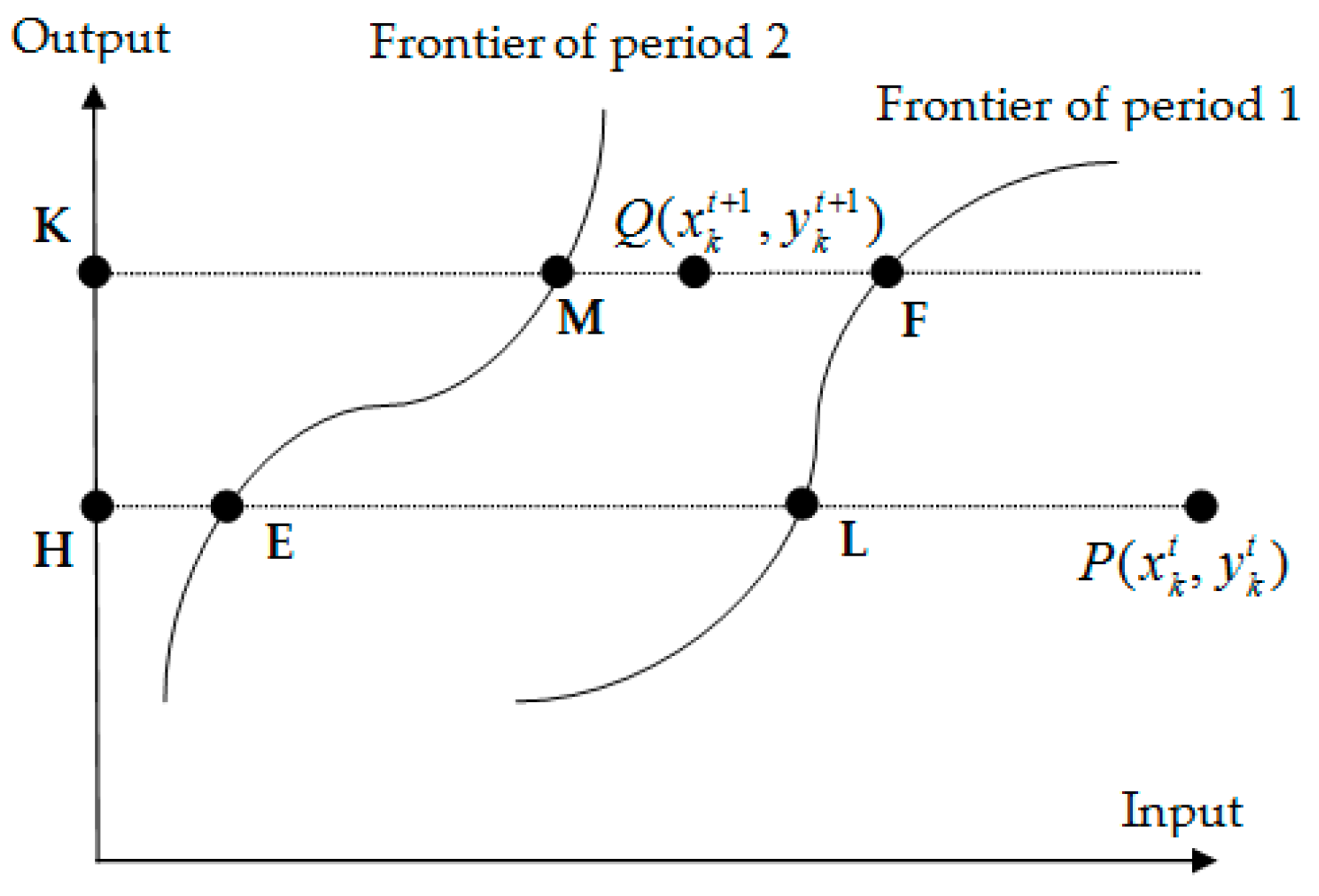
18]. In this study, the authors evaluated the technical, technology, and business efficiency of the consultants, design, and construction contractors of traffic infrastructure between the two periods P ( x k t , y k t ) and Q ( x k t + 1 , y k t + 1 ) (as shown in Figure 2). In it, the catch-up index (ECA) is used to evaluate the technical efficiency of the contractor. The frontier-shift index (EFR) is used to evaluate the technology efficiency of the contractors. The Malmquist productivity index (EMPI) is used to evaluate the performance of contractors.
The ECA, EFR, and EMPI indexes are used to evaluate the technical efficiency, technology efficiency, and business performance of investors at time (t + 1) is the point Q ( x k t + 1 , y k t + 1 ) , score for where t is the point P ( x k t , y k t ) is calculated by the following formula.
ECA = KM KQ × HP HL = [ D k t + 1 ( x k t + 1 , y k t + 1 ) D k t ( x k t , y k t ) ]
EFR = HL HE × KF KM = [ D k t ( x k t + 1 , y k t + 1 ) D k t + 1 ( x k t + 1 , y k t + 1 ) × D k t ( x k t , y k t ) D k t + 1 ( x k t , y k t ) ] 1 2
EMPI = ECA × EFR                     = [ D k t + 1 ( x k t + 1 , y k t + 1 ) D k t ( x k t , y k t ) ] × [ D k t ( x k t + 1 , y k t + 1 ) D k t + 1 ( x k t + 1 , y k t + 1 ) × D k t ( x k t , y k t ) D k t + 1 ( x k t , y k t ) ] 1 2
In particular:
The efficiency of investors at point ( x k t , y k t ) period t is determined by the following formula [19]:
D k t ( x k t , y k t ) = Max φ k t
j = 1 n λ j x i j t x i k t ,   j = 1 ,   2 ,   3 , ,   m
j = 1 n λ j y r j t φ k t y r k t ,   r = 1 ,   2 ,   3 , ,   s
λ j 0
The efficiency of investors at point ( x k t , y k t ) period t + 1 is determined by the following formula [19]:
D k t + 1 ( x k t , y k t ) = Max φ k t + 1
j = 1 n λ j x i j t + 1 x i k t ,   j = 1 ,   2 ,   3 , ,   m
j = 1 n λ j y r j t + 1 φ k t + 1 y r k t ,   r = 1 ,   2 ,   3 , ,   s
λ j 0
The efficiency of investors at point ( x k t + 1 , y k t + 1 ) period t is determined by the following formula [19]:
D k t ( x k t + 1 , y k t + 1 ) = Max φ k t
j = 1 n λ j x i j t + 1 x i k t ,   j = 1 ,   2 ,   3 , ,   m
j = 1 n λ j y r j t φ k t y r k t + 1 ,   r = 1 ,   2 ,   3 , ,   s
λ j 0
The efficiency of investors at point ( x k t + 1 , y k t + 1 ) period t + 1 is determined by the following formula [19]:
D k t + 1 ( x k t + 1 , y k t + 1 ) = Max φ k t + 1
j = 1 n λ j x i j t + 1 x i k t + 1 ,   j = 1 ,   2 ,   3 , ,   m
j = 1 n λ j y r j t + 1 φ k t + 1 y r k t + 1 ,   r = 1 ,   2 ,   3 , ,   s
λ j 0
If the ECA, EFR, EMPI indexes are less than 1 (<1), this reflects that the technical, technological, and financial investment of the consultants, and design and construction contractors in the traffic layer during the assessment period were not effective. If these indicators are greater than 1 (>1), it is clear that the bids achieved the above three indicators during this period. These indicators are equal to 1 (=1) reflecting the performance in the comparison period corresponding to the previous period [20].

3.2.4. Correlation Coefficients

The correlation coefficient (k), first introduced in 1895, is a statistical tool used to test correlations between variables. The formula for calculating the correlation coefficient is as follows [21]:
k = i = 1 n ( α i α ¯ ) ( δ i δ ¯ ) [ i = 1 n ( α i α ¯ ) 2 i = 1 n ( δ i δ ¯ ) 2 ] 1 2
The value of k depends on the range (−1; 1). The value of negative k denotes the inverse relationship between the two factors (if the value of this factor increases, then the other factor decreases and vice versa). The value of positive k denotes the positive correlation between the two factors (if the value of this factor increases, the value of the other factor increases; if this value decreases, the value of the other factor will decrease accordingly). The value of k = 0 denotes independent factors [22].

4. Results

4.1. Forecasting

Designing and executing traffic infrastructure works for the period 2018–2021, the authors use data from factor F1 of I12 (Table 7) to explain the computational steps in the GM (1, 1) model used in this study (as follows).
From the original data range: X ( 0 ) = ( 4032.71 ; 3941.09 ; 4615.74 ; 4187.99 )
Use the accumulating generation operation method to compute X(1) values:
X ( 1 ) = ( 4032.71 ; 7973.80 ; 12589.54 ; 16777.53 )
Calculate the mean values Z(1): Z ( 1 ) = ( 6003.26 ; 10281.67 ; 14683.53 )
From the values of X(0), Z(1) the authors obtain the following system of equations:
{ 3941.0853 + a × 6003.26 = b 4615.7374 + a × 10281.67 = b 4187.9907 + a × 14683.53 = b
From the above equations, transformed into the matrix form as follows:
B = [ 6003.26 10281.67 14683.53 ] ;   Y Ν = [ 3941.0853 4615.7374 4187.9907 ]
[ а b ] = [ 0.0278 3960.8791 ]
Use the values a and b to find the differential equation:
d x ( k ) ( 1 ) d t 0.0278 x ( 0 ) = 3960.8791
Equation prediction:
x ^ ( k + 1 ) ( 1 ) = ( 4032.71 + 3960.8791 0.0278 ) × e 0.0278 k 3960.8791 0.0278 = 146510.3755 × e 0.0278 k 142477.6655
In turn, the values for k = 0, 1, 2, ..., 7 are given, x ^ ( k + 1 ) ( 1 ) by the following values:
x ^ ( k + 1 ) ( 1 ) = { 4032.71 ; 8163.09 ; 12410.08 ; 16776.97 ; 21267.14 ; 25884.08 ; 30631.36 ; 35512.66 }
Use the accumulating generation operation method to calculate the predicted values by the formula: x ^ ( k + 1 ) ( 0 ) = x ^ ( k + 1 ) ( 1 ) x ^ k ( 1 ) obtains the predicted values for the years in Table 8.
As calculated above, the authors obtained predictive values for all elements of bidders for the period 2018–2021 which are summarized in Table 9, Table 10, Table 11 and Table 12 below:
To test the accuracy of the predicted values, the authors used MAPE to ensure that the results of this study were highly reliable. The results in Table 13 are as follows:
As shown in Table 13, average all In = 6.94% indicates that the forecasts for contractors’ business performance for the period 2018–2021 are high. In particular, the predicted data for 4/17 of contractors ranged from 10 to 20%, while the predicted data for 13 of 17 contractors had errors of less than 10%. This confirms that the GM (1, 1) model used to predict the contractor’s business performance in this study is consistent with high reliability.

4.2. Correlation Coefficient

The correlation coefficients are shown in Table 14. Based on the convention mentioned in Section 3.2.4, it was found that the factors used in this study were positive (the increase in inputs would lead to the increase in output). This is in line with economic law. All coefficients are greater than 0.6, indicating that these factors have a strong correlation.
This result shows that the data used in this study are consistent with the conditions of use of the optimal mathematical models used in this study. The conclusions of the study have sufficient grounds for assessing the technical, technological, and economic efficiency of contractors in the field of construction of transport infrastructure works.
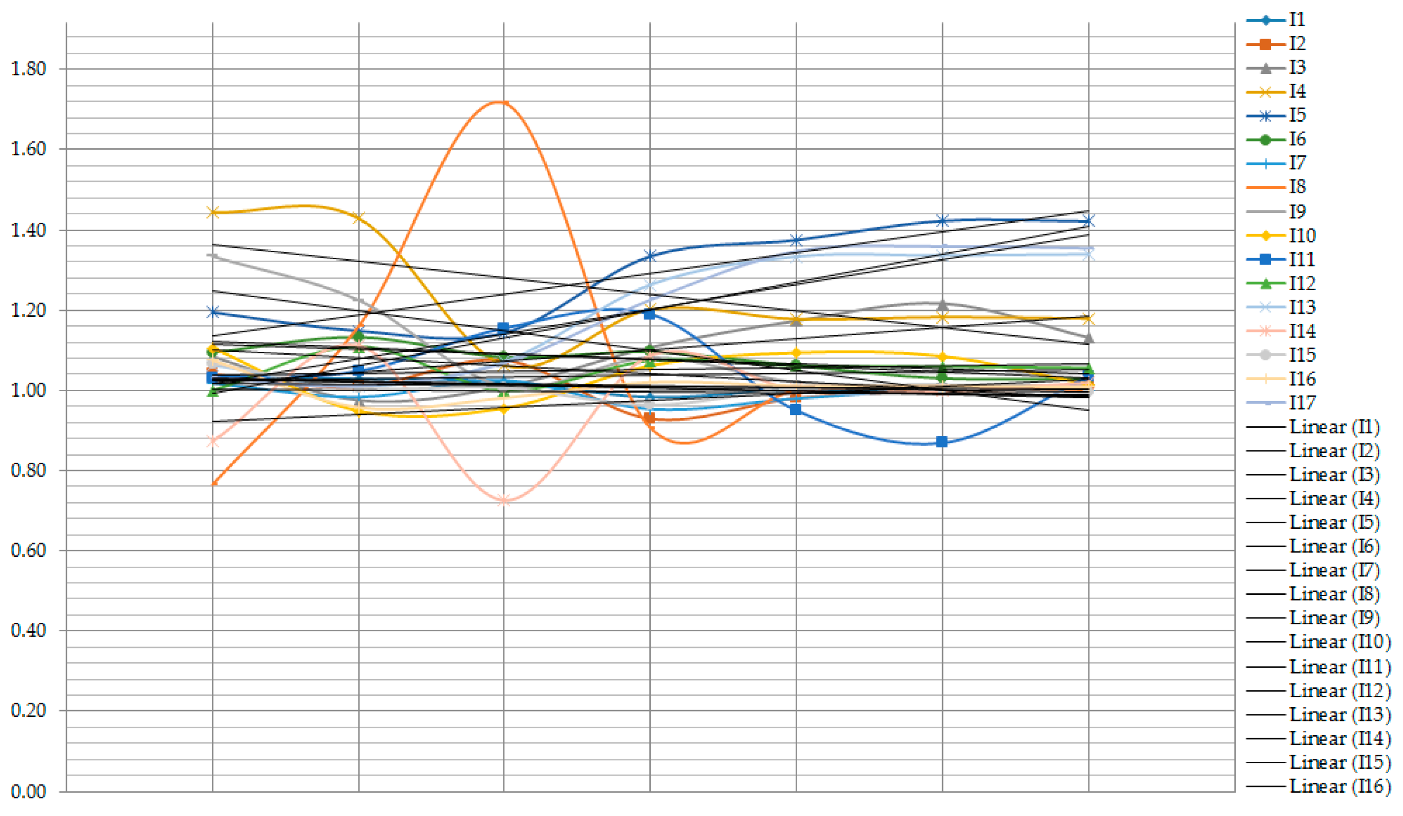
4.3. Catch-Up Index

The catch-up index reflects the technical efficiency of the consultants, design, and construction contractors for transport infrastructure in Vietnam for the period 2014–2021, as shown in Table 15.
The results in Table 15 and Figure 3 show that the consultants, design, and construction of transport infrastructure have not achieved technical efficiency in the period 2013–2017. Specifically, the catch-up index in this phase is less than 1 (average ECA 2014–2015 = 0.9782; average ECA 2015–2016 = 0.9933; average ECA 2016–2017 = 0.9945). However, according to the results above, in the period 2017–2020, the contractor has made changes and achieved technical efficiency. In the period 2017–2020, the catch-up index is greater than 1 (average ECA 2017–2018 = 1.0085; average ECA 2018–2019 = 1.0051; average ECA 2019–2020 = 1.0091). In particular, there are strong changes and high efficiency of three contractors (I1, I11, I15). These bidders have not really achieved technical efficiency in the period 2014–2017, but, from the period 2017–2021, there are solutions to create efficiency (catch-up index is greater than 1). In addition, nine out of 17 contractors have maintained stable technical performance in the period 2017–2021, including I4, I5, I6, I7, I8, I9, I12, I13, I17. However, many contractors have not yet achieved technical efficiency (I1, I2, I10, I14, I16). Managers rely on this result to set up timely measures, in line with the actual situation, to improve the technical efficiency of their businesses in the future.
In construction, machinery is always a decisive factor in productivity, quality, and efficiency. Therefore, the frequent research and development of new high-tech techniques play a decisive role. On the other hand, the machinery and equipment in construction are typically of great economic value; further, the maintenance of machinery and equipment, ensuring the machinery is always operating properly and takes advantage of the capacity of machinery equipment, plays a huge role in improving the technical efficiency of contractors.
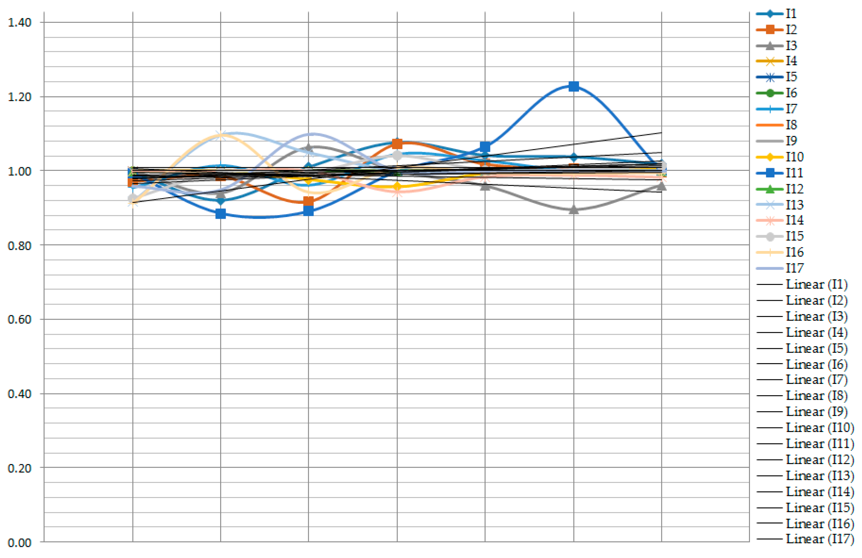
4.4. Frontier Index

The CFR index reflects the technological efficiency of construction contractors for transport infrastructure development. The results in Table 16 show that the technology efficiency scores of past contractors (2014–2017) and future predictions (2018–2021) are good. Specifically, the average technology efficiency scores for bidders for the period 2014–2021 are average 2014–2015: 1.0744; average 2015–2016: 1.0764; average 2016–2017: 1.0656; average 2017–2018:1.0872; average 2018–2019: 1.0928; average 2019–2020: 1.0936; average 2020–2021: 1.0955.
Based on the results of the technology efficiency score of the contractors, as shown in Table 16 and Figure 4, the authors created three groups:
  • Highly efficient bidders in the future, including I3, I4, I5, I6, I9, I10, I12, I13, I16, I17. These bidders are expected to have a technology efficiency score greater than 1 (>1) over the period 2018–2021.
  • Contractors that maintain stable technology in the future, including I8. This contractor is expected to be technologically stable (=1) over the period 2018–2021.
  • Contractors not effective in terms of technology in the future, including I1, I2, I7, I11, I14, I15. These bidders are predicted to be technologically efficient with high volatility during the period 2018–2021.
In general, construction contractors of transport works in Vietnam have approached and mastered modern technologies, improving the capacity of construction of transport works to meet the requirements of construction works. Along with that is the use of high-quality materials and application of new technology to bring high economic efficiency and longevity for the works.

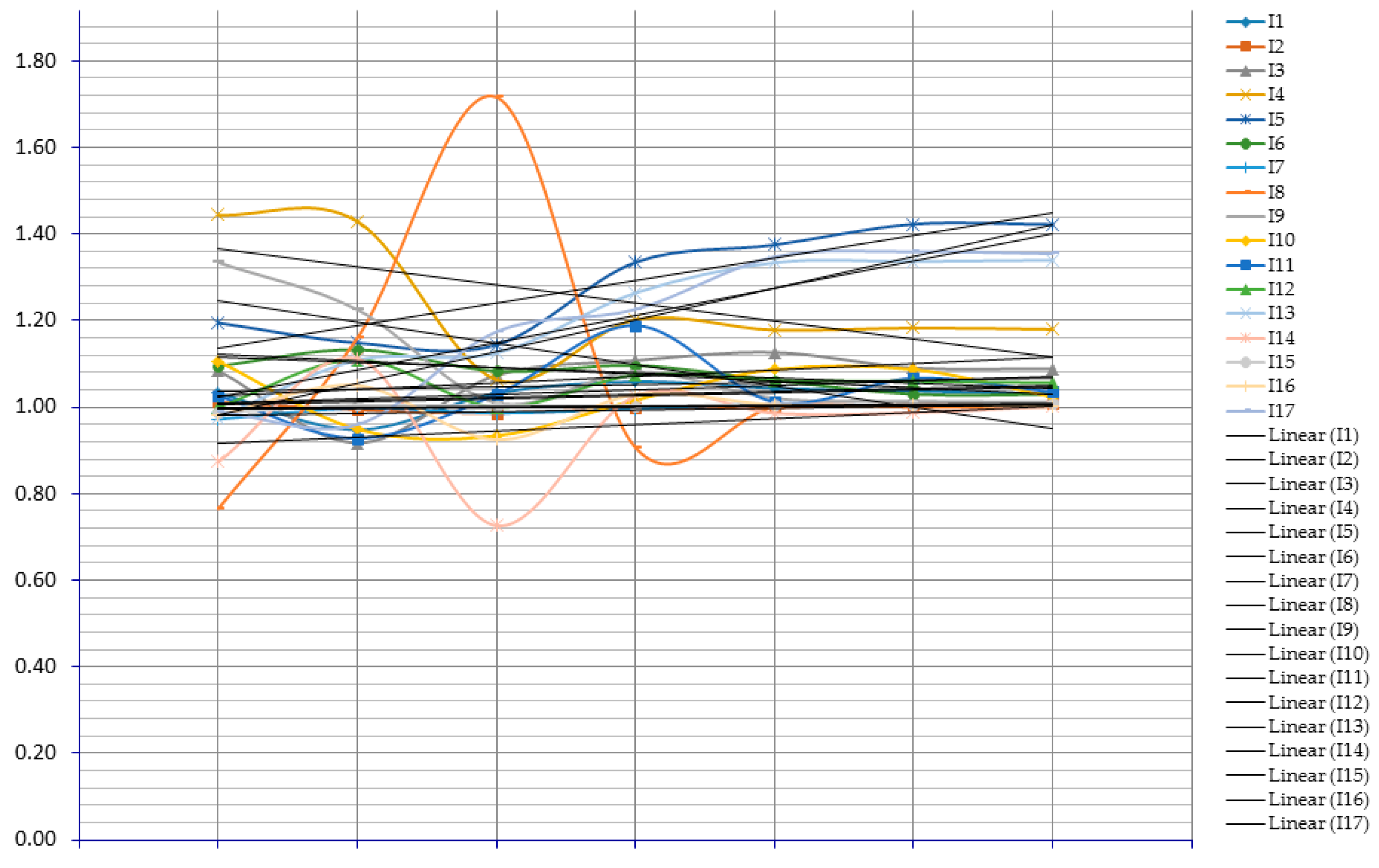
4.5. Malmquist Index

As shown in Table 17 and Figure 5, EMPI average 2014–2018 = 1.0807, which reflects the business performance of the contractor of traffic works in general and is quite satisfactory. Specifically, according to the forecast results, in the period 2018–2021, 13 out of 17 contractors have achieved high business results, including I1, I3, I4, I5, I6, I9, I10, I11, I12, I13, I15, I16, I17. In addition, 2/17 contractors are expected to maintain stable business performance during this period, including I7, I8. However, 2/17 of the contractors whose business results are forecasted to be ineffective include I2, I14.
In order to maintain and improve business efficiency, contractors themselves must actively create, overcome difficulties, promote advantages, and exploit and make use of favorable conditions and factors of the environment and geographic location, thus combining multiple measures to maximize the use of resources and businesses to achieve optimal efficiency. The economic efficiency of production and business activities in consultancy, design, and construction of traffic works is an integrated category in many fields. In order to improve the economic efficiency of production and business activities, contractors must use the combination of measures from raising the management capacity and managing production and business activities of enterprises in the office to work. In addition to enhancing and improving all the activities within the enterprise, enterprises are always adapting to the changes of the market, i.e., adaptation to each project in different localities. Bidders must regularly maintain and ensure the balance of the relationship between parties from the construction site, so the new office can enhance the sense of responsibility of each person, i.e., enhance the initiative in production to bring high economic efficiency.

4.6. Contractor Selection

The results of forecasting and evaluating the technical, technological, and business efficiency of the consultants, design, and construction contractors of the transport infrastructure are shown in Table 18.
Based on these results, the government, regulatory authorities in strategy formulation, policy development, selection of consultants, and design and construction contractors have good capacity to implement projects. It is of decisive importance in ensuring the progress and quality of traffic works. The result of this business performance assessment is also a good basis for all self-revising subjects, to see where their businesses are in the overall picture of the construction investment sector to provide timely solutions to improve capacity and more effective implementation of assigned tasks.

5. Conclusions

At present, with the rapid development of the economy, demand for transportation and transportation of goods and people remains large. As a result, road, rail, waterway, and air infrastructure works are being increasingly built. Therefore, the role of contractor consulting, design, and construction of transport infrastructure has become more important and maintains a special position. The main contractor is the decisive factor affecting the quality and progress of construction of the transportation infrastructure. In this study, the authors used a modern, highly accurate forecasting method to forecast contractors’ business, design, and construction contractor performance. Also, in this study, the authors used optimized mathematical models to evaluate past, present, and future contractors’ technical, technological, and performance effectiveness. The result of this study is a solid basis for the government, regulatory agencies, and investors to use for strategic planning and policy development of transport infrastructure with high efficiency. The best way to do this is through the selection of contractors who have the human, financial, technical, and technological capabilities to meet the requirements of managers and investors.
In addition to the results achieved, this research still has certain limitations: It does not combine with the qualitative factors, weather factors, and government policies. In addition, many of the optimal mathematical models have not been considered in this study. The authors will continue to address these issues in subsequent studies.

Author Contributions

C.-N.W. developed and checked theoretical calculations. T.-M.L. wrote and formatted the manuscript. H.-K.N. contributed to analyzing the data. All authors have read and accepted this research.

Funding

This research received no external funding.

Conflicts of Interest

The authors declare no conflict of interest.

References

  1. Yang, J.B.; Wang, W.C. Contractor selection by the most advantageous tendering approach in Taiwan. J. Chin. Inst. Eng. 2003, 26, 381–387. [Google Scholar] [CrossRef]
  2. Holt, G.D. Which contractor selection methodology? Int. J. Proj. Manag. 1998, 16, 153–164. [Google Scholar] [CrossRef]
  3. Zhou, P.A.B.W.; Ang, B.W.; Poh, K.L. A trigonometric grey prediction approach to forecasting electricity demand. Energy 2006, 31, 2839–2847. [Google Scholar] [CrossRef]
  4. Zhao, Z.; Wang, J.; Zhao, J.; Su, Z. Using a Grey model optimized by Differential Evolution algorithm to forecast the per capita annual net income of rural households in China. Omega 2012, 40, 525–532. [Google Scholar] [CrossRef]
  5. Shi, G.M.; Bi, J.; Wang, J.N. Chinese regional industrial energy efficiency evaluation based on a DEA model of fixing non-energy inputs. Energy Policy 2010, 38, 6172–6179. [Google Scholar] [CrossRef]
  6. Pilyavsky, A.; Staat, M. Efficiency and productivity change in Ukrainian health care. J. Prod. Anal. 2008, 29, 143–154. [Google Scholar] [CrossRef]
  7. Wang, C.N.; Nguyen, H.K.; Liao, R.Y. Partner Selection in Supply Chain of Vietnam’s Textile and Apparel Industry: The Application of a Hybrid DEA and GM (1,1) Approach. Math. Probl. Eng. 2017. [Google Scholar] [CrossRef]
  8. Shuai, J.J.; Wu, W.W. Evaluating the influence of E-marketing on hotel performance by DEA and grey entropy. Expert Syst. Appl. 2011, 38, 8763–8769. [Google Scholar] [CrossRef]
  9. Minh-Hue, N. Logistics Vietnam report 2017. Available online: http://nhaxuatbancongthuong.com (accessed on 21 May 2018).
  10. Statistics. General Statistics Office of Vietnam. Available online: https://www.gso.gov.vn (accessed on 25 May 2018).
  11. Deng, J. Control problems of grey systems. Syst. Control Lett. 1982, 1, 288–294. [Google Scholar]
  12. Wang, C.N.; Nguyen, H.K. Enhancing Urban Development Quality Based on the Results of Appraising Efficient Performance of Investors—A Case Study in Vietnam. Sustainability 2017, 9, 1397. [Google Scholar] [CrossRef]
  13. Boles, J.-S.; Donthu, N.; Ritu, L. Salesperson evaluation using relative performance efficiency: The application of data envelopment analysis. J. Pers. Sell. Sales Manag. 1995, 15, 31–49. [Google Scholar]
  14. Charnes, A.; Cooper, W.-W.; Rhodes, E. Evaluating Program and Managerial Efficiency: An Application of Data Envelopment Analysis to Program Follow Through. Manag. Sci. 1981, 27, 668–697. [Google Scholar] [CrossRef]
  15. Banker, R.-D.; Charnes, A.; Cooper, W.-W. Some models for estimating technical and scale inefficiencies in data envelopment analysis. Manag. Sci. 1984, 30, 1078–1092. [Google Scholar] [CrossRef]
  16. Mao, W.; Koo, W.W. Productivity growth, technological progress, and efficiency change in chinese agriculture after rural economic reforms: A DEA approach. China Econ. Rev. 1997, 8, 157–174. [Google Scholar] [CrossRef]
  17. Macpherson, A.-J.; Principe, P.-P.; Mehaffey, M. Using Malmquist Indices to evaluate environmental impacts of alternative land development scenarios. Ecological Indicators 2013, 34, 296–303. [Google Scholar] [CrossRef]
  18. Paradi, J.C.; Asmild, M.; Aggarwall, V.; Schaffnit, C. Performance Evaluation in an Oligopoly Environment: Combining DEA Window Analysis with the Malmquist Index Approach—A Study of the Canadian Banking Industry; Centre for Management of Technology and Entrepreneurship University of Toronto, University of Toronto: Toronto, ON, Canada, 2011; pp. 31–47. [Google Scholar]
  19. Odeck, J. Identifying traffic safety best practice: An application of DEA and Malmquist indices. Omega 2006, 34, 28–40. [Google Scholar] [CrossRef]
  20. Wang, C.N.; Nguyen, N.T.; Tran, T.T. Integrated DEA Models and Grey System Theory to Evaluate Past-to-Future Performance: A Case of Indian Electricity Industry. Sci. World J. 2015. [Google Scholar] [CrossRef] [PubMed]
  21. Wang, J. Pearson Correlation Coefficient. In Encyclopedia of Systems Biology; Springer: New York, NY, USA, 2013; pp. 97–141. [Google Scholar]
  22. Nahler, G. Pearson correlation coefficient. In Dictionary of Pharmaceutical Medicine; Springer: Vienna, Austria, 2017. [Google Scholar]
Figure 1. Contractor selection procedure [1].
Mathematics 07 00098 g001
Figure 2. Catch-up terms [18].
Mathematics 07 00098 g002
Figure 3. Catch-up index.
Mathematics 07 00098 g003
Figure 4. Frontier index.
Mathematics 07 00098 g004
Figure 5. Malmquist index.
Mathematics 07 00098 g005
Table 1. Road infrastructure.
OrderType of RoadsTotal RouteTotal Length (km)
1Highways13745
2Route14623,816
3Provincial road99827,176
4District roads868057,294
5Commune roads61,402173,294
6Urban road23,49527,910
7Other rural roads168,888256,377
8Specialized road24768528
Source: [9].
Table 2. List of contractors.
InCompanies
I1Construction joint stock company No. 1
I2HUD3 investment and construction joint stock company
I3Construction joint stock company No. 9
I4Coteccons construction joint stock company
I5Hoa Binh construction group joint stock company
I6Binhduong trade and development joint stock company
I7Development investment construction Hoi An joint stock company
I8Licogi 14 joint stock company
I9Tien Giang investment and construction joint stock company
I10Construction joint stock company No. 5
I11Chuong Duong joint stock company
I12Constrexim No 8 investment and construction joint stock company
I13Vietnam Construction joint stock company No. 2
I14Binh Duong construction and civil engineering joint stock company
I15HUD1 investment & construction joint stock company
I16Vinaconex 6 joint stock company
I17Sci E&C joint stock company
Source: [10].
Table 3. Data in 2014.
InF1F2F3F4F5F6
I127,619.7110,642.9818,457.90937.68515.4220,056.04
I228,709.947639.4813,874.53829.40555.5315,705.79
I369,303.228152.7525,489.891355.45492.2329,433.26
I4213,612.52111,010.37310,891.739433.0915,701.84335,310.80
I5254,920.9143,753.02136,519.4612,303.893021.07154,538.01
I6275,092.3951,467.3161,864.002470.024951.2076,694.83
I78965.292328.1011,151.77415.67132.4811,794.35
I823,157.622239.677996.86179.96830.199456.81
I917,820.806940.1019,197.121141.27747.3023,063.05
I1096,207.6014,653.4657,300.18956.571465.0961,143.84
I1135,509.2611,122.299447.72526.14348.9911,005.28
I124032.711130.605697.05100.9457.375866.17
I1370,769.7611,952.0023,135.132340.04729.6026,622.03
I1441,732.9315,413.3325,252.74273.30941.0226,854.88
I1532,607.107802.0130,375.07986.96334.7631,927.61
I1623,968.934944.8324,042.54874.82342.8825,566.41
I1712,052.332929.928139.35582.72357.699618.24
Source: [10].
Table 4. Data in 2015.
InF1F2F3F4F5F6
I125,427.8710,544.9815,046.55546.92524.6916,143.51
I227,240.897804.6016,308.62935.70690.6418,736.61
I358,661.128387.8426,583.991288.07486.5633,167.85
I4343,282.14142,430.07551,576.2515,936.9232,188.75600,414.22
I5320,271.1047,193.66210,066.595260.523638.61223,054.97
I6323,038.5052,527.0650,531.612336.354789.3768,593.61
I79782.042316.949064.47454.06131.649783.93
I821,538.002982.7226,301.02372.01896.4828,106.62
I926,452.398868.8324,122.091319.392460.3130,724.63
I1099,017.4713,671.1159,662.10788.291571.2662,866.42
I1135,416.7511,524.7412,789.79594.80753.0615,497.41
I123941.091127.264227.08115.5743.884402.08
I1368,716.4712,154.7626,534.481686.70649.7529,570.57
I1478,950.4515,484.4920,196.87307.351107.0122,297.69
I1527,798.577888.8026,135.77892.70368.3227,642.07
I1623,237.084712.9422,131.74746.43102.2123,132.23
I1715,926.255473.4710,984.45731.45617.4212,838.24
Source: [10].
Table 5. Data in 2016.
InF1F2F3F4F5F6
I135,109.2710,485.6822,603.281134.68564.1424,390.61
I226,796.597970.6422,050.171076.09703.6424,479.21
I360,403.748407.8334,716.181268.74609.5537,280.20
I4515,723.84273,815.34833,852.1213,056.9962,468.41912,891.79
I5502,938.3180,390.64418,775.3916,586.7124,950.27472,911.18
I6319,702.3553,657.3045,777.732306.885634.8163,677.86
I710,255.382320.899588.46493.99147.5910,267.46
I819,557.493960.067722.72374.111183.629963.19
I930,463.4912,107.5928,276.701286.453799.4736,441.09
I1087,299.6814,039.2561,030.95945.631841.6264,615.23
I1132,274.4112,500.7611,130.81568.00710.4512,491.93
I124615.741132.185321.93125.0142.965497.76
I13111,536.6912,839.0339,513.772294.981322.2945,818.27
I1455,524.6215,639.8636,510.14341.96678.3437,868.28
I1528,725.277715.3415,890.36485.60142.0116,929.51
I1630,738.164943.1130,534.96847.72332.3831,949.23
I1724,888.245590.8813,841.111338.85177.0215,710.31
Source: [10].
Table 6. Data in 2017.
InF1F2F3F4F5F6
I135,716.5010,548.0124,608.441811.97666.6127,375.57
I232,613.608584.3214,505.261242.48842.6717,305.95
I374,012.578369.1743,573.891199.83553.8146,708.38
I4697,419.42320,950.061,104,166.3417,331.8272,594.781,192,729.49
I5614,888.03108,362.54630,370.5920,780.7737,798.35704,445.13
I6345,556.5654,166.4940,539.082031.605903.7259,339.64
I710,254.632289.537539.38476.64105.868201.51
I813,150.606368.549517.91658.882767.7914,748.52
I937,817.7214,129.2630,026.082179.234033.5939,965.81
I1088,450.1815,173.5481,247.452393.502634.7486,402.59
I1141,387.1512,037.268806.98599.721272.6110,050.29
I124187.991135.785589.87135.0743.225772.25
I1399,261.0813,428.6981,743.763821.781348.6092,106.15
I1450,846.6915,659.8424,190.22410.001286.7125,434.63
I1542,474.187645.8122,175.67749.19230.3523,825.16
I1635,662.034940.5225,106.20795.23329.7926,310.29
I1732,817.246018.8135,321.301315.83673.6938,384.97
Source: [10].
Table 7. Data of I12.
YearF1F2F3F4F5F6
20144032.711130.605697.05100.9457.375866.17
20153941.091127.264227.08115.5743.884402.08
20164615.741132.185321.93125.0142.965497.76
20174187.991135.785589.87135.0743.225772.25
Table 8. Forecast data F1 of I12.
Year20142015201620172018201920202021
Forecast4032.714130.384246.994366.894490.174616.944747.284881.30
Table 9. Forecast data in 2018.
InF1F2F3F4F5F6
I143,148.9710,529.2631,583.343002.34743.7835,590.60
I234,876.688937.0116,084.481427.70914.9518,918.35
I381,722.918369.6555,330.651166.97616.7554,842.26
I4970,992.39464,410.491,528,230.1517,007.63105,075.321,645,842.91
I5837,908.16158,089.651,010,373.1335,425.9980,927.611,146,236.67
I6352,912.6655,106.4336,489.401941.596626.5255,128.51
I710,574.942281.917373.88497.44106.198000.74
I811,396.459067.292843.32861.834424.966251.14
I944,823.1417,802.4933,790.762746.825195.6545,802.04
I1081,267.2315,874.3192,890.063753.243361.3299,281.31
I1143,105.1812,531.787512.81592.521623.518090.65
I124490.171140.296514.66145.9542.706697.85
I13124,451.9114,130.21132,385.345576.551904.47149,909.49
I1437,470.9615,770.6130,520.06469.611254.6131,322.63
I1551,484.787509.4617,234.57555.00116.7818,751.01
I1644,165.085095.4828,770.26844.86526.5430,174.41
I1745,949.206265.7955,965.601772.24573.3960,413.53
Table 10. Forecast data in 2019.
InF1F2F3F4F5F6
I150,268.7610,530.7839,335.965135.68841.4045,135.29
I238,405.699380.6515,372.271645.091016.0318,323.39
I392,406.668360.3570,525.621126.83653.5465,455.69
I41,362,850.22652,348.512,123,825.3617,859.22147,332.032,274,415.58
I51,128,340.52231,141.551,650,867.0957,935.96161,765.741,892,158.68
I6365,367.8355,956.3832,713.771815.377327.1251,272.07
I710,823.352268.446785.52509.1696.747383.38
I89129.5013,497.171389.641206.798428.183906.00
I953,806.6922,183.5437,561.503691.756451.8152,051.24
I1076,607.5916,738.56109,851.237293.264420.41117,992.54
I1147,016.9512,796.426273.92595.052228.476521.79
I124616.941144.597428.14157.7742.377609.37
I13144,387.2214,849.66241,883.958566.412532.30272,267.60
I1429,524.4115,859.3932,487.51544.201392.9232,828.68
I1565,218.217392.4015,507.31492.6782.5517,042.17
I1654,172.455215.0730,323.31870.30770.0831,838.47
I1764,451.776575.94111,382.722242.08621.99115,378.84
Table 11. Forecast data in 2020.
InF1F2F3F4F5F6
I158,563.3510,532.3048,991.598784.90951.8357,239.69
I242,291.799846.3114,691.591895.591128.2617,747.14
I3104,487.138351.0789,893.441088.07692.5378,123.11
I41,912,847.87916,341.452,951,541.1318,753.45206,582.563,143,049.80
I51,519,441.39337,950.122,697,381.8594,748.97323,352.643,123,494.98
I6378,262.5856,819.4429,328.811697.368101.7847,685.40
I711,077.602255.056244.11521.1788.136813.66
I87313.4820,091.29679.171689.8116,053.072440.64
I964,590.7527,642.7141,753.014961.748011.6759,153.09
I1072,215.1117,649.85129,909.4114,172.205813.20140,230.21
I1151,283.7013,066.655239.32597.593058.845257.15
I124747.281148.908469.72170.5642.058644.94
I13167,515.8715,605.75441,951.1013,159.303367.09494,496.04
I1423,263.1115,948.6834,581.79630.641546.4934,407.14
I1582,615.007277.1613,953.15437.3558.3515,489.06
I1666,447.395337.4831,960.20896.511126.2933,594.31
I1790,404.866901.43221673.892836.48674.71220,352.59
Table 12. Forecast data in 2021.
InF1F2F3F4F5F6
I168,226.5910,533.8261,017.3415,027.111076.7672,590.24
I246,571.1110,335.0914,041.062184.231252.9017,189.01
I3118,146.888341.79114,580.071050.65733.8493,242.00
I42,684,804.911,287,167.274,101,841.5419,692.46289,661.074,343,428.75
I52,046,104.07494,114.034,407,301.41154,953.26646,347.785,156,132.51
I6391,612.4257,695.8226,294.101587.028958.3544349.63
I711,337.822241.745745.90533.4580.286287.90
I85858.7029,907.01331.942366.1730,576.111525.03
I977,536.1634,445.3546,412.266668.629948.6667,223.91
I1068,074.4918,610.76153,630.0927,539.307644.83166,658.94
I1155,937.6613,342.594375.34600.144198.644237.74
I124881.301153.249657.34184.3741.739821.43
I13194,349.3716,400.33807,497.8720,214.664477.08898,110.26
I1418,329.6516,038.4636,811.08730.801716.9836,061.50
I15104,652.347163.7112,554.75388.2441.2414,077.50
I1681,503.715462.7633,685.45923.511647.2535,446.97
I17126,808.597243.04441,175.363588.46731.90420,833.36
Table 13. Errors results.
InMAPE (%)InMAPE (%)
I13.82I105.12
I25.01I113.73
I31.92I121.78
I45.38I136.85
I515.13I149.90
I60.99I1513.16
I73.35I168.08
I813.55I1716.47
I93.80Average all In (%)6.94
Table 14. Correlation coefficient.
Time Period 2014Time Period 2015
F1F2F3F4F5F6F1F2F3F4F5F6
F11.000.810.710.790.670.731.000.850.750.750.680.76
F20.811.000.960.770.970.960.851.000.960.970.960.96
F30.710.961.000.830.961.000.750.961.000.990.961.00
F40.790.770.831.000.670.840.750.970.991.000.970.99
F50.670.970.960.671.000.960.680.960.960.971.000.96
F60.730.961.000.840.961.000.760.961.000.990.961.00
Time Period 2016Time Period 2017
F11.000.830.870.920.850.871.000.890.920.930.920.92
F20.831.000.970.770.990.970.891.000.970.810.980.96
F30.870.971.000.880.991.000.920.971.000.920.991.00
F40.920.770.881.000.840.890.930.810.921.000.900.93
F50.850.990.990.841.000.990.920.980.990.901.000.99
F60.870.971.000.890.991.000.920.961.000.930.991.00
Table 15. The catch-up index.
(ECA)‘14–‘15‘15–‘16‘16–‘17‘17–‘18‘18–‘19‘19–‘20‘20–‘21Average
I10.99560.92111.01041.07681.04191.03801.01801.0146
I20.97180.98550.91721.07261.01791.00630.99630.9954
I31.00000.94041.06341.00000.95990.89610.96200.9745
I41.00001.00001.00001.00001.00001.00001.00001.0000
I51.00001.00001.00001.00001.00001.00001.00001.0000
I61.00001.00001.00001.00001.00001.00001.00001.0000
I70.95461.01450.96161.04501.02761.00001.00001.0005
I81.00001.00001.00001.00001.00001.00001.00001.0000
I91.00001.00001.00001.00001.00001.00001.00001.0000
I101.00001.00000.97690.95710.99361.00141.00880.9911
I110.99350.88560.89110.99881.06541.22721.00001.0088
I121.00001.00001.00001.00001.00001.00001.00001.0000
I130.91671.09661.04901.00001.00001.00001.00001.0089
I141.00001.00001.00000.94370.98410.98820.98280.9855
I150.92560.99670.99601.04101.00171.00411.01320.9969
I160.91211.09630.94241.00880.99470.99360.99500.9919
I170.95880.94911.09891.00001.00001.00001.00001.0010
Average0.97820.99330.99451.00851.00511.00910.99860.9982
Max1.00001.09661.09891.07681.06541.22721.01801.0146
Min0.91210.88560.89110.94370.95990.89610.96200.9745
SD0.03230.05230.04990.03420.02320.06260.01200.0092
Table 16. Frontier index.
(EFR)‘14–‘15‘15–‘16‘16–‘17‘17–‘18‘18–‘19‘19–‘20‘20–‘21Average
I11.03681.02911.02200.98331.00170.99901.01241.0120
I21.04071.00871.07530.92970.98131.00061.01281.0070
I31.08440.97561.00961.10781.17371.21701.13201.1000
I41.44381.42941.06331.20181.17801.18311.17991.2399
I51.19491.14851.14391.33451.37501.42271.42201.2917
I61.09481.13291.08301.09651.06161.03011.02931.0755
I71.01830.98361.02560.95360.98021.00201.00050.9948
I80.76541.15971.71640.90661.00001.00001.00001.0783
I91.33441.22531.01001.08201.02041.01381.01191.0997
I101.10630.94910.95581.06191.09431.08551.01471.0382
I111.03291.04801.15541.19020.94990.86921.03521.0401
I121.00001.10961.00001.07431.06211.05991.05621.0517
I131.06371.01081.07231.26391.33391.33651.33961.2030
I140.87331.11190.72631.08721.00170.99911.01930.9741
I151.06721.00711.00690.96401.00431.00250.99471.0067
I161.07570.95800.98141.02021.01121.01061.00871.0094
I171.03211.01111.06851.22591.34741.35901.35451.1998
Average1.07441.07641.06561.08721.09281.09361.09551.0836
Max1.44381.42941.71641.33451.37501.42271.42201.2917
Min0.76540.94910.72630.90660.94990.86920.99470.9741
SD0.15230.12100.19200.12310.13890.15450.14150.0946
Table 17. Malmquist index.
(EMPI)‘14–‘15‘15–‘16‘16–‘17‘17–‘18‘18–‘19‘19–‘20‘20–‘21Average
I11.03220.94801.03261.05881.04361.03701.03071.0261
I21.01140.99410.98630.99720.99891.00701.00901.0005
I31.08440.91741.07361.10781.12661.09051.08901.0699
I41.44381.42941.06331.20181.17801.18311.17991.2399
I51.19491.14851.14391.33451.37501.42271.42201.2917
I61.09481.13291.08301.09651.06161.03011.02931.0755
I70.97210.99790.98620.99651.00721.00201.00050.9946
I80.76541.15971.71640.90661.00001.00001.00001.0783
I91.33441.22531.01001.08201.02041.01381.01191.0997
I101.10630.94910.93381.01631.08721.08701.02361.0290
I111.02620.92811.02961.18881.01201.06671.03521.0409
I121.00001.10961.00001.07431.06211.05991.05621.0517
I130.97511.10851.12481.26391.33391.33651.33961.2118
I140.87331.11190.72631.02600.98580.98721.00180.9589
I150.98781.00381.00291.00351.00601.00661.00781.0026
I160.98121.05030.92501.02921.00581.00411.00370.9999
I170.98950.95971.17411.22591.34741.35901.35451.2014
Average1.05131.06911.05951.09471.09721.09961.09381.0807
Max1.44381.42941.71641.33451.37501.42271.42201.2917
Min0.76540.91740.72630.90660.98580.98721.00000.9589
SD0.15900.13160.19740.11280.13180.13970.14070.0973
Table 18. Classify contractor.
Good EfficiencyEfficiencyInefficiency
ECAI1, I11, I15I4, I5, I6, I7, I8, I9, I12, I13, I17I2, I3, I10, I14, I16
EFRI3, I4, I5, I6, I9, I10, I12, I13, I16, I17I8I1, I2, I7, I11, I14, I15
EMPII1, I3, I4, I5, I6, I9, I10, I11, I12, I13, I15, I16, I17I7, I8I2, I14

