Exact Solution for the Heat Transfer of Two Immiscible PTT Fluids Flowing in Concentric Layers through a Pipe

Abstract

This article investigates the heat transfer flow of two layers of Phan-Thien-Tanner (PTT) fluids though a cylindrical pipe. The flow is assumed to be steady, incompressible, and stable and the fluid layers do not mix with each other. The fluid flow and heat transfer equations are modeled using the linear PTT fluid model. Exact solutions for the velocity, flow rates, temperature profiles, and stress distributions are obtained. It has also been shown that one can recover the Newtonian fluid results from the obtained results by putting the non-Newtonian parameters to zero. These results match with the corresponding results for Newtonian fluids already present in the literature. Graphical analysis of the behavior of the fluid velocities, temperatures, and stresses is also presented at the end. It is also shown that maximum velocity occurs in the inner fluid layer.

1. Introduction

Two-layer flows of non-Newtonian fluids are frequently encountered in industry, manufacturing processes, and oil transportation etc. A considerable amount of work on stratified laminar flow of two immiscible viscous fluids in horizontal parallel plates and circular pipes exists in the literature in an effort to find the possibilities of reducing input to transport low density fluids such as crude oil by adding high-density fluid such as water [1]. Moreover, it was observed in various real-life situations such as in oceans and in seas where salty water does not mix with water coming from glaciers due to differences in densities and viscosities, resulting in fluids flowing side by side and in layers [2]. Packham and Shail [3] studied the stratified laminar flow of two immiscible viscous fluids in a pipe. They have expressed velocity distribution in terms of two separate pipe-flow solutions. They have also calculated flow rates and some other quantities. Brauner [4] analyzed the annular-core flow of two immiscible liquids to obtain the results for pressure-loss reduction and power-saving in the transportation of very viscous oils. Considerable efforts by [5,6,7] have been made to model the two-phase magnetohydrodynamic heat transfer flow of Newtonian fluids in pumps and MHD generators. The results are presented for suitable ratios of depths and viscosities. Apart from the planar channel geometry, an inclined channel is also considered in [1]. Leib et al. studied the two-layer flow of Newtonian fluids in an annular geometry in [8]. Siddiqui et al. [9] studied the problem of concentric n layer flows of viscous fluids in a pipe. They have presented exact solutions of velocity profiles and volume flow rates, showing that a unique maximum velocity always exists in the core of the pipe for any number of fluid layers. Newtonian fluids have extensively been analyzed for the above-mentioned problems of multi-layer flows but they have limited applications in technological processes. Since most of the phenomena occurring in the real world are complex, Newtonian fluids fail to represent such phenomena. Non-Newtonian fluids best describe the nature of such real-life processes and are therefore well suited for application in industries. These fluids are therefore industrially important and exhibit rheological properties such as viscoelasticity. Some common examples of their usage are in the chemical, dyeing, food, and petroleum industries.

Among the rheological models for non-Newtonian fluids, the viscoelastic models allow a more realistic prediction of the physical phenomena related to the fluid flow. Such fluids can be described by many complex constitute equations, i.e., The Phan-Thien-Tanner (PTT) model, The Giesekus model, The Leonov model, and pom-pom model [10]. Here we take two different PTT fluids to study immiscible fluid flow. Examples of PTT fluids are fluids exhibiting viscoelastic behavior such as polymer solutions and melts, oil, clay, toothpaste etc.. The present work deals with the heat transfer in two concentric layers of PTT fluids flowing in a pipe, if the fluid interface is ripple-free and plane.

The paper is organized as follows: Section 2 contains the governing equations of the fluid model. In Section 3 the problem under consideration is formulated. In Section 4, a solution to the problem is given. In Section 5, the graphical results and discussion of the problem is provided. Section 6 contains conclusions.

2. Basic Equations

The basic equations governing the non-isothermal flow of two immiscible, incompressible fluids are the continuity equation, the law of conservation of momentum, and the law of conservation of energy. Mathematically,

$$\begin{array}{ccc}\hfill div{\mathbf{V}}^{(k)}& =& 0,k=1,2,\hfill \end{array}$$

(1)

$$\begin{array}{ccc}\hfill {\rho }^{(k)}{\displaystyle \frac{d{\mathbf{V}}^{(k)}}{dt}}& =& div{\mathit{\tau }}^{(k)}-gradp+{\rho }^{(k)}\mathbf{b},k=1,2,\hfill \end{array}$$

(2)

$$\begin{array}{ccc}\hfill {\rho }^{(k)}{c}_p^{(k)}{\displaystyle \frac{d{\mathsf{\Theta }}^{(k)}}{dt}}& =& {\kappa }^{(k)}{\nabla }^2{\mathsf{\Theta }}^{(k)}+{\mathbf{T}}^{(k)}·{\mathbf{L}}^{(k)};k=1,2,\hfill \end{array}$$

(3)

where the superscript k denotes the two fluids, the number $k=1$ represents the fluid in the core, while the fluid properties for the outer fluid along the pipe wall are denoted by the superscript $k=2$. ${\rho }^{(k)}$ is the constant fluid density, ${\mathbf{V}}^{(k)}$ is the velocity vector, ${\mathit{\tau }}^{(k)}$ is the extra stress tensor, $c_p^{(k)}$ is the specific heat of the fluid, ${\mathsf{\Theta }}^{(k)}$ denotes temperature of the fluid, ${\kappa }^{(k)}$ represents the thermal conductivity, p is dynamic pressure, ${\mathbf{T}}^{(k)}=-p\mathbf{I}+{\mathit{\tau }}^{(k)}$ is the Cauchy stress tensor of the kth fluid, and $\mathbf{b}$ is the body force per unit mass, ${\displaystyle \frac{d}{dt}}$ denotes the material time derivative, ${\mathbf{L}}^{(k)}$ is the gradient of ${\mathbf{V}}^{(k)}$. The general form of the constitutive equation defining the PTT fluid is

$$f\left(tr({\mathit{\tau }}^{(k)})\right){\mathit{\tau }}^{(k)}+{\lambda }^{(k)}{\widehat{\mathit{\tau }}}^{(k)}=2{\eta }^{(k)}{\mathbf{A}}_1^{(k)};k=1,2,$$

(4)

where ${\eta }^{(k)}$ and ${\lambda }^{(k)}$ are the coefficient of viscosity and relaxation time of the kth fluid, $tr({\mathit{\tau }}^{(k)}$ is the trace of stress tensor ${\mathit{\tau }}^{(k)}$ and ${\mathbf{A}}_1^{(k)}$ is the deformation rate tensor defined by

$${\mathbf{A}}_1^{(k)}={\displaystyle \frac{1}{2}}\left[{\mathbf{L}}^{(k)}+{({\mathbf{L}}^{(k)})}^T\right];k=1,2.$$

(5)

The upper convected derivative term ${\widehat{\mathit{\tau }}}^{(k)}$ can be expressed as

$${\widehat{\mathit{\tau }}}^{(k)}={\displaystyle \frac{d{\mathit{\tau }}^{(k)}}{dt}}-{\mathit{\tau }}^{(k)}·{\mathbf{L}}^{(k)}-{({\mathbf{L}}^{(k)})}^T·{\mathit{\tau }}^{(k)};k=1,2.$$

(6)

According to Tanner’s classification [11], a linear form of the function f in the PTT model is

$$f\left(tr({\mathit{\tau }}^{(k)})\right)=1+{\displaystyle \frac{{\epsilon }^{(k)}{\lambda }^{(k)}}{{\eta }^{(k)}}}tr({\mathit{\tau }}^{(k)});k=1,2,$$

(7)

where ${\epsilon }^{(k)}$ is a parameter related to the elongational behavior of the fluid model. In the absence of the parameter ${\epsilon }^{(k)}$, the model (4) reduces to the well-known Maxwell model.

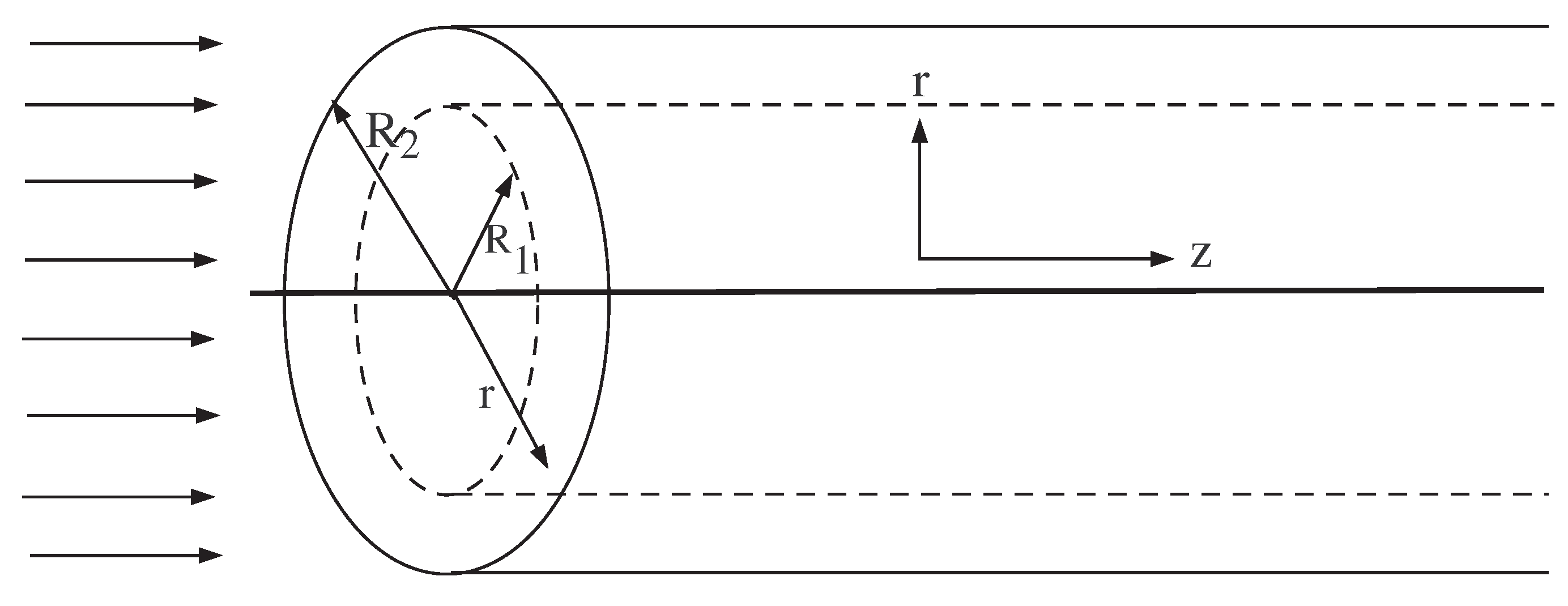
3. Problem Formulation

We consider the concentric unidirectional flow of two immiscible, incompressible PTT fluids in a cylindrical pipe as shown in the figure (see Figure 1). The horizontal pipe of radius $R_2$ is kept at a constant temperature $\mathsf{\Theta }$. The interface of the two fluids lies at a constant distance $R_1$ from the axis of the pipe. The geometry of the problem facilitates the choice of cylindrical coordinates system for its representation. Therefore, we choose $z-$axis to be at the axis of the pipe while r is measured radially outward from the axis. We can therefore assume that

Figure 1. The geometry of the problem.

The flow is driven by a constant pressure gradient. We assume that the flow is steady, unidirectional, and fully developed. The velocities and extra stresses are assumed to be of the form

$${\mathbf{V}}^{(k)}=[0,0,u^{(k)}(r)],\mathrm{and}{\mathit{\tau }}^{(k)}={\mathit{\tau }}^{(k)}(r);k=1,2.$$

(8)

By substituting these relations into the continuity Equation (1) and into the momentum and energy Equations (2) and (3), we find that the continuity equation is identically satisfied while the other two, in the absence of body forces, yield

$r$—component of the momentum equation

$${\displaystyle \frac{\partial p}{\partial r}}-{\displaystyle \frac{1}{r}}{\displaystyle \frac{d}{dr}}\left(r{\tau }_{rr}^{(k)}\right)=0;k=1,2,$$

(9)

$\theta$—component of the momentum equation

$${\displaystyle \frac{1}{r}}{\displaystyle \frac{\partial p}{\partial \theta }}-{\displaystyle \frac{1}{r^2}}{\displaystyle \frac{d}{dr}}\left(r^2{\tau }_{r\theta }^{(k)}\right)=0;k=1,2,$$

(10)

$z$—component of the momentum equation

$${\displaystyle \frac{\partial p}{\partial z}}-{\displaystyle \frac{1}{r}}{\displaystyle \frac{d}{dr}}\left(r{\tau }_{rz}^{(k)}\right)=0;k=1,2,$$

(11)

and energy equation

$${\displaystyle \frac{{\kappa }^{(k)}}{r}}{\displaystyle \frac{d}{dr}}\left(r{\displaystyle \frac{d{\mathsf{\Theta }}^{(k)}}{dr}}\right)+{\tau }_{rz}^{(k)}\left({\displaystyle \frac{d{u}^{(k)}}{dr}}\right)=0;k=1,2.$$

(12)

Upon substitution the relation in (8) into the constitutive Equations (4)–(7), we find that the only nonzero components of the stress tensor are given by

$$\begin{array}{ccc}\hfill \left(1+{\displaystyle \frac{{\epsilon }^{(k)}{\lambda }^{(k)}}{{\eta }^{(k)}}}tr({\mathit{\tau }}^{(k)})\right){\tau }_{rz}^{(k)}& =& {\eta }^{(k)}{\displaystyle \frac{d{u}^{(k)}}{dr}};k=1,2,\hfill \end{array}$$

(13)

$$\begin{array}{ccc}\hfill \left(1+{\displaystyle \frac{{\epsilon }^{(k)}{\lambda }^{(k)}}{{\eta }^{(k)}}}tr({\mathit{\tau }}^{(k)})\right){\tau }_{zz}^{(k)}& =& 2{\lambda }^{(k)}{\tau }_{rz}^{(k)}{\displaystyle \frac{d{u}^{(k)}}{dr}};k=1,2.\hfill \end{array}$$

(14)

In view of the zero components of the extra stress tensor, Equations (9)–(11) reduce to

$$\begin{array}{ccc}\hfill {\displaystyle \frac{\partial p}{\partial r}}& =& 0,\hfill \end{array}$$

(15)

$$\begin{array}{ccc}\hfill {\displaystyle \frac{\partial p}{\partial \theta }}& =& 0,\hfill \end{array}$$

(16)

$$\begin{array}{ccc}\hfill {\displaystyle \frac{\partial p}{\partial z}}& =& {\displaystyle \frac{1}{r}}{\displaystyle \frac{d}{dr}}\left(r{\tau }_{rz}^{(k)}\right);k=1,2.\hfill \end{array}$$

(17)

Equations (15) and (16) further imply that $p=p(z)$ only so that we can write Equation (17) as

$${\displaystyle \frac{dp}{dz}}={\displaystyle \frac{1}{r}}{\displaystyle \frac{d}{dr}}\left(r{\tau }_{rz}^{(k)}\right);k=1,2.$$

(18)

Furthermore, from Equations (13) and (14), and the fact that $tr({\tau }^{(k)})={\tau }_{zz}^{(k)},$ we find that

$${\tau }_{zz}^{(k)}=2{\displaystyle \frac{{\lambda }^{(k)}}{{\eta }^{(k)}}}{{\tau }_{rz}^{(k)}}^2;k=1,2.$$

(19)

Putting the value of ${\tau }_{zz}^{(k)}$ in (13), we obtain the constitutive equation

$${\tau }_{rz}^{(k)}+2{\displaystyle \frac{{\epsilon }^{(k)}{{\lambda }^{(k)}}^2}{{{\eta }^{(k)}}^2}}{{\tau }_{rz}^{(k)}}^3={\eta }^{(k)}{\displaystyle \frac{d{u}^{(k)}}{dr}};k=1,2.$$

(20)

for the particular problem.

3.1. Boundary Conditions

The boundary conditions for the problem under consideration are for

• Shear Stresses

  $$\begin{array}{ccc}\hfill {\tau }_{rz}^{(1)}& =& 0,\mathrm{at}r=0(\mathrm{symmetry} \mathrm{about} z-\mathrm{axis}),\hfill \end{array}$$

  (21)

  $$\begin{array}{ccc}\hfill {\tau }_{rz}^{(1)}& =& {\tau }_{rz}^{(2)},\mathrm{at}r=R_1(\mathrm{continuity} \mathrm{of} \mathrm{shear} \mathrm{stresses}).\hfill \end{array}$$

  (22)
• Velocities

  $$\begin{array}{ccc}\hfill u^{(1)}& =& u^{(2)},\mathrm{at}r=R_1(\mathrm{continuity} \mathrm{of} \mathrm{velocities}),\hfill \end{array}$$

  (23)

  $$\begin{array}{ccc}\hfill u^{(2)}& =& 0,\mathrm{at}r=R_2(\mathrm{no-slip} \mathrm{at} \mathrm{the} \mathrm{wall}).\hfill \end{array}$$

  (24)
• Temperatures

  $$\begin{array}{ccc}\hfill {\displaystyle \frac{d{\mathsf{\Theta }}^{(1)}}{dr}}& =& 0,\mathrm{at}r=0(\mathrm{symmetry} \mathrm{about} z-\mathrm{axis}),\hfill \end{array}$$

  (25)

  $$\begin{array}{ccc}\hfill {\kappa }^{(1)}{\displaystyle \frac{d{\mathsf{\Theta }}^{(1)}}{dr}}& =& {\kappa }^{(2)}{\displaystyle \frac{d{\mathsf{\Theta }}^{(2)}}{dr}},\mathrm{at}r=R_1(\mathrm{continuity} \mathrm{of} \mathrm{temperatures}),\hfill \end{array}$$

  (26)

  $$\begin{array}{ccc}\hfill {\mathsf{\Theta }}^{(1)}& =& {\mathsf{\Theta }}^{(2)},\mathrm{at}r=R_1(\mathrm{continuity} \mathrm{of} \mathrm{temperatures}),\hfill \end{array}$$

  (27)

  $$\begin{array}{ccc}\hfill {\mathsf{\Theta }}^{(2)}& =& {\mathsf{\Theta }}_o,\mathrm{at}r=R_2(\mathrm{temperature} \mathrm{of} \mathrm{the} \mathrm{wall}e).\hfill \end{array}$$

  (28)

Here it is noticed that these conditions are eight in number and are sufficient to find solution to the problem comprising of two first order differential equations represented by (18), two first order differential equations represented by (20), and the two second order differential equations given by (12). Hence, our problem is consistent and can be solved exactly.

3.2. Dimensionless Parameter

For the problem under consideration we introduce the following dimensionless parameters:

$$\begin{array}{ccc}\hfill r^{*}& =& {\displaystyle \frac{r}{R_2}},z^{*}={\displaystyle \frac{z}{R_2}},u^{*(k)}={\displaystyle \frac{u^{(k)}}{U}},p^{*}={\displaystyle \frac{p{R}_2}{{\eta }^{(1)}U}},{\tau }_{ij}^{*(k)}={\displaystyle \frac{{\tau }_{ij}^{(k)}}{{\eta }^{(1)}{\displaystyle \frac{U}{R_2}}}},\hfill \\ \hfill {\eta }^{(k)*}& =& {\displaystyle \frac{{\eta }^{(k)}}{{\eta }^{(1)}}},{\lambda }^{(k)*}={\displaystyle \frac{{\lambda }^{(k)}U}{R_2}},{\theta }^{*(k)}={\displaystyle \frac{{\theta }^{(k)}-{\theta }_w}{{\theta }_0-{\theta }_w}},{\kappa }^{(k)*}={\displaystyle \frac{{\kappa }^{(k)}}{{\kappa }^{(1)}}},\mathrm{and}\xi ={\displaystyle \frac{R_1}{R_2}},\hfill \end{array}$$

(29)

where U, $R_2$, ${\kappa }^{(1)}$ and ${\eta }^{(1)}$ are assumed to be characteristic velocity, radius, thermal conductivity, and viscosity, respectively.

4. Solution of the Problem

4.1. Stress Distributions

Introducing dimensionless parameters (29) in expressions (18), (21) and (22) and after dropping the “∗” we get the dimensionless form of Equation (18) as given:

$${\displaystyle \frac{dp}{dz}}={\displaystyle \frac{1}{r}}{\displaystyle \frac{d}{dr}}\left(r{\tau }_{rz}^{(k)}\right);k=1,2.$$

(30)

together with dimensionless boundary conditions

$$\begin{array}{ccc}\hfill {\tau }_{rz}^{(1)}& =& 0,\mathrm{at}r=0,\hfill \end{array}$$

(31)

$$\begin{array}{ccc}\hfill {\tau }_{rz}^{(1)}& =& {\tau }_{rz}^{(2)},\mathrm{at}r=\xi .\hfill \end{array}$$

(32)

Equation (30), upon integration with respect to r, yields

$$r{\tau }_{rz}^{(k)}={\displaystyle \frac{dp}{dz}}{\displaystyle \frac{r^2}{2}}+A^{(k)};k=1,2,$$

(33)

where $A^{(k)},k=1,2$ are constants of integration. Using the condition (31) in Equation (33) when $k=1$, we find that $A^{(1)}=0$, so that we obtain

$${\tau }_{rz}^{(1)}={\displaystyle \frac{dp}{dz}}{\displaystyle \frac{r}{2}};0\le r\le \xi .$$

(34)

Similarly, we make use of condition (32) for solving (33) when $k=2$ and find that $A^{(2)}=0$. This results in the expression

$${\tau }_{rz}^{(2)}={\displaystyle \frac{dp}{dz}}{\displaystyle \frac{r}{2}};\xi \le r\le 1.$$

(35)

The expression (34) and (35) clearly indicate that the shear stresses of both the fluids are same and vary linearly with distance from the axis. This results in the expression

$${\tau }_{rz}^{(k)}={\displaystyle \frac{dp}{dz}}{\displaystyle \frac{r}{2}};k=1,2.$$

(36)

This relation for ${\tau }_{rz}$ agrees with the one presented in [9] for Newtonian fluids. The last result, when used in Equation (19) for normal stresses, implies that

$${\tau }_{zz}^{(k)}={\displaystyle \frac{{\lambda }^{(k)}}{2{\eta }^{(k)}}}{\left({\displaystyle \frac{dp}{dz}}\right)}^2{r}^2;k=1,2.$$

(37)

The expression (37) suggests that the normal stresses for both the fluids are different, depending on their corresponding material constants, even though both the fluids experience the same pressure gradient. Moreover, these normal stresses increase with the square of the distance from the axis of the tube. To deduce the results for Newtonian fluids as a special case, we substitute ${\lambda }^{(1)}={\lambda }^{(2)}=0$ in expressions (36) and (37) and find that the shear stress distributions remain unchanged while the normal stresses are zero for both the fluids.

4.2. Velocity Profile

Using the expressions (34) and (35) in (20), we find that for velocity profiles, the first order differential Equation (20) assume the form

$${\displaystyle \frac{d{u}^{(k)}}{dr}}={\displaystyle \frac{1}{2{\eta }^{(k)}}}{\displaystyle \frac{dp}{dz}}r+{\displaystyle \frac{{\epsilon }^{(k)}{\lambda }^{{(k)}^2}}{4{\eta }^{{(k)}^3}}}{\left({\displaystyle \frac{dp}{dz}}\right)}^3{r}^3;k=1,2.$$

(38)

Introducing dimensionless parameters (29) in Equations (38), (23) and (24) and after dropping the “∗” we get the dimensionless form of Equation (38) together with boundary conditions as given below:

$${\displaystyle \frac{d{u}^{(k)}}{dr}}={\displaystyle \frac{1}{2{\eta }^{(k)}}}{\displaystyle \frac{dp}{dz}}r+{\displaystyle \frac{{\epsilon }^{(k)}{\lambda }^{{(k)}^2}}{4{\eta }^{{(k)}^3}}}{\left({\displaystyle \frac{dp}{dz}}\right)}^3{r}^3;k=1,2.$$

(39)

$$\begin{array}{ccc}\hfill u^{(1)}& =& u^{(2)},\mathrm{at}r=\xi ,\hfill \end{array}$$

(40)

$$\begin{array}{ccc}\hfill u^{(2)}& =& 0,\mathrm{at}r=1.\hfill \end{array}$$

(41)

Integrating both sides of Equation (39) with respect to r, we obtain

$$u^{(k)}={\displaystyle \frac{1}{4{\eta }^{(k)}}}{\displaystyle \frac{dp}{dz}}{r}^2+{\displaystyle \frac{{\epsilon }^{(k)}{\lambda }^{{(k)}^2}}{16{\eta }^{{(k)}^3}}}{\left({\displaystyle \frac{dp}{dz}}\right)}^3{r}^4+B^{(k)};k=1,2,$$

(42)

where $B^{(k)},k=1,2$ are constants of integration. Equation (42) for $k=2$ becomes

$$u^{(2)}={\displaystyle \frac{1}{4{\eta }^{(2)}}}{\displaystyle \frac{dp}{dz}}{r}^2+{\displaystyle \frac{{\epsilon }^{(2)}{\lambda }^{{(2)}^2}}{16{\eta }^{{(2)}^3}}}{\left({\displaystyle \frac{dp}{dz}}\right)}^3{r}^4+B^{(2)}.$$

(43)

Using the no-slip condition (41), we evaluate $B^{(2)}$ and then using this value of $B^{(2)}$ in Equation (43), we finally obtain the value of $u^{(2)}$ which is given by

$$u^{(2)}={\displaystyle \frac{1}{4{\eta }^{(2)}}}\left(-{\displaystyle \frac{dp}{dz}}\right)\left(1-r^2\right)+{\displaystyle \frac{{\epsilon }^{(2)}{\lambda }^{{(2)}^2}}{16{\eta }^{{(2)}^3}}}{\left(-{\displaystyle \frac{dp}{dz}}\right)}^3\left(1-r^4\right);\xi \le r\le 1.$$

(44)

Expression (44) for $u^{(2)}$ and the boundary condition (40) help to find the value of $B^{(1)}$, the constant arising in (42) for $k=1$. After this value of $B^{(1)}$ is substituted back into Equation (42), the final expression for velocity $u^{(1)}$ comes out to be

$$\begin{array}{ccc}\hfill u^{(1)}& =& {\displaystyle \frac{1}{4{\eta }^{(1)}}}\left(-{\displaystyle \frac{dp}{dz}}\right)\left({\xi }^2-r^2\right)+{\displaystyle \frac{{\epsilon }^{(1)}{\lambda }^{{(1)}^2}}{16{\eta }^{{(1)}^3}}}{\left(-{\displaystyle \frac{dp}{dz}}\right)}^3\left({\xi }^4-r^4\right)\hfill \\ \hfill & +& {\displaystyle \frac{1}{4{\eta }^{(2)}}}\left(-{\displaystyle \frac{dp}{dz}}\right)\left(1-{\xi }^2\right)+{\displaystyle \frac{{\epsilon }^{(2)}{\lambda }^{{(2)}^2}}{16{\eta }^{{(2)}^3}}}{\left(-{\displaystyle \frac{dp}{dz}}\right)}^3\left(1-{\xi }^4\right);0\le r\le \xi .\hfill \end{array}$$

(45)

We can deduce the results for Newtonian fluids by substituting ${\lambda }^{(1)}={\lambda }^{(2)}=0$ in (44) and (45) as

$$\begin{array}{ccc}\hfill u^{(1)}& =& {\displaystyle \frac{1}{4{\eta }^{(1)}}}\left(-{\displaystyle \frac{dp}{dz}}\right)\left({\xi }^2-r^2\right);0\le r\le \xi ,\hfill \end{array}$$

(46)

$$\begin{array}{ccc}\hfill u^{(2)}& =& {\displaystyle \frac{1}{4{\eta }^{(2)}}}\left(-{\displaystyle \frac{dp}{dz}}\right)\left(1-r^2\right);\xi \le r\le 1.\hfill \end{array}$$

(47)

These results from Equations (46) and (47) agree with those presented in [9] for Newtonian fluids. Similarly, we can deduce the expression for velocities when one of the two fluids is Newtonian in nature by substituting the $\lambda$ corresponding to that fluid equal to zero.

4.3. Maximum Velocity

Maximum velocity in the kth layer occurs at a point where

$${\displaystyle \frac{d{u}^{(k)}}{dr}}=0,{\displaystyle \frac{d^2{u}^{(k)}}{d{r}^2}}<0\mathrm{for}{r}_{k+1}<r<r_{k;}(r_1=1)k=1,2,\cdots ,n-1.$$

(48)

In our case we observe that

$${\displaystyle \frac{d{u}^{(1)}}{dr}}=0;k=1,$$

(49)

if and only if $r=0$. The following relation also holds

$${\left[{\displaystyle \frac{d^2{u}^{(1)}}{d{r}^2}}\right]}_{r=0}={\displaystyle \frac{1}{2{\eta }^{(1)}}}{\displaystyle \frac{dp}{dz}}<0.$$

(50)

This shows that a unique velocity maximum exists in the 1st fluid layer, which is the innermost fluid layer, i.e., core of the pipe. Equation (45) clearly shows that the maximum velocity depends on the applied pressure gradient as well as on all the viscosity coefficients.

4.4. Total Volume Flow Rate through a Cross Section of the Pipe

The total volumetric flow rate Q in dimensionless form (after dropping the “∗”) is given by the sum

$$Q=\sum _{k=1}^2{Q}^{(k)},k=1,2.$$

(51)

where ${\displaystyle \frac{Q}{R_2^{2}U}}=Q^{*}$.

$$Q^{(2)}=2\pi \underset{\xi }{\overset{1}{\int }}r{u}^{(2)}(r)dr,\xi \le r\le 1,\mathrm{flow} \mathrm{rate} \mathrm{in} \mathrm{the} \mathrm{outer} \mathrm{layer},$$

(52)

$$Q^{(1)}=2\pi \underset{0}{\overset{\xi }{\int }}r{u}^{(1)}(r)dr,0\le r\le \xi ,\mathrm{flow} \mathrm{rate} \mathrm{in} \mathrm{the} \mathrm{inner} \mathrm{layer}.$$

(53)

Using Equations (44) and (45) in Equations (52) and (53), we get

$$Q^{(2)}={\displaystyle \frac{\pi }{8{\eta }^{(2)}}}\left(-{\displaystyle \frac{dp}{dz}}\right)\left(1-2{\xi }^2+{\xi }^4\right)+{\displaystyle \frac{\pi {\epsilon }^{(2)}{\lambda }^{{(2)}^2}}{48{\eta }^{{(2)}^3}}}{\left(-{\displaystyle \frac{dp}{dz}}\right)}^3\left(2-3{\xi }^2+{\xi }^6\right);\xi \le r\le 1.$$

(54)

and

$$\begin{array}{ccc}\hfill Q^{(1)}& =& {\displaystyle \frac{\pi }{8{\eta }^{(1)}}}\left(-{\displaystyle \frac{dp}{dz}}\right){\xi }^4+{\displaystyle \frac{\pi {\epsilon }^{(1)}{\lambda }^{{(1)}^2}}{24{\eta }^{{(1)}^3}}}{\left(-{\displaystyle \frac{dp}{dz}}\right)}^3{\xi }^6+{\displaystyle \frac{\pi }{4{\eta }^{(2)}}}\left(-{\displaystyle \frac{dp}{dz}}\right)\left({\xi }^2-{\xi }^4\right)\hfill \\ \hfill & +& {\displaystyle \frac{\pi {\epsilon }^{(2)}{\lambda }^{{(2)}^2}}{16{\eta }^{{(2)}^3}}}{\left(-{\displaystyle \frac{dp}{dz}}\right)}^3\left({\xi }^2-{\xi }^6\right);0\le r\le \xi .\hfill \end{array}$$

(55)

4.5. Temperature Distributions

Using the values of ${\tau }_{rz}^{(1)}$ and ${\tau }_{rz}^{(2)}$ from (34) and (35) respectively in (12) we find that

$${\displaystyle \frac{{\kappa }^{(k)}}{r}}{\displaystyle \frac{d}{dr}}\left(r{\displaystyle \frac{d{\mathsf{\Theta }}^{(k)}}{dr}}\right)+{\displaystyle \frac{dp}{dz}}{\displaystyle \frac{r}{2}}\left({\displaystyle \frac{d{u}^{(k)}}{dr}}\right)=0;k=1,2.$$

(56)

We note here that the viscous dissipation terms are nonzero and play an important role in the heat equation. Introducing dimensionless parameters (29) in Equation (56) and after dropping ∗ we get

$${\displaystyle \frac{1}{r}}{\displaystyle \frac{d}{dr}}\left(r{\displaystyle \frac{d{\mathsf{\Theta }}^{(k)}}{dr}}\right)+{\displaystyle \frac{1}{{\kappa }^{(k)}}}Br{\displaystyle \frac{dp}{dz}}{\displaystyle \frac{r}{2}}\left({\displaystyle \frac{d{u}^{(k)}}{dr}}\right)=0;k=1,2,$$

(57)

where $Br={\displaystyle \frac{{\eta }^{(1)}{U}^2}{{\kappa }^{(1)}({\theta }_0-{\theta }_w)}}$ is the Brinkman number.

Boundary conditions for temperature distribution, (25)–(28), after dropping “∗” become

$$\begin{array}{ccc}\hfill {\displaystyle \frac{d{\mathsf{\Theta }}^{(1)}}{dr}}& =& 0,\mathrm{at}r=0,\hfill \end{array}$$

(58)

$$\begin{array}{ccc}\hfill {\kappa }^{(1)}{\displaystyle \frac{d{\mathsf{\Theta }}^{(1)}}{dr}}& =& {\kappa }^{(2)}{\displaystyle \frac{d{\mathsf{\Theta }}^{(2)}}{dr}},\mathrm{at}r=\xi ,\hfill \end{array}$$

(59)

$$\begin{array}{ccc}\hfill {\mathsf{\Theta }}^{(1)}& =& {\mathsf{\Theta }}^{(2)},\mathrm{at}r=\xi ,\hfill \end{array}$$

(60)

$$\begin{array}{ccc}\hfill {\mathsf{\Theta }}^{(2)}& =& {\mathsf{\Theta }}_o,\mathrm{at}r=1.\hfill \end{array}$$

(61)

After using Equation (39) in (57) and making some simplifications, we reach at the following second order differential equations

$${\displaystyle \frac{d}{dr}}\left(r{\displaystyle \frac{d{\mathsf{\Theta }}^{(k)}}{dr}}\right)+{\displaystyle \frac{Br}{4{\kappa }^{(k)}{\eta }^{(k)}}}{\left({\displaystyle \frac{dp}{dz}}\right)}^2{r}^3+{\displaystyle \frac{Br{\epsilon }^{(k)}{\lambda }^{{(k)}^2}}{8{\kappa }^{(k)}{\eta }^{(k)3}}}{\left({\displaystyle \frac{dp}{dz}}\right)}^4{r}^5=0;k=1,2.$$

(62)

Integrating (62) with respect to r, we get

$$r{\displaystyle \frac{d{\mathsf{\Theta }}^{(k)}}{dr}}=-{\displaystyle \frac{Br}{16{\kappa }^{(k)}{\eta }^{(k)}}}{\left({\displaystyle \frac{dp}{dz}}\right)}^2{r}^4-{\displaystyle \frac{Br{\epsilon }^{(k)}{\lambda }^{{(k)}^2}}{48{\kappa }^{(k)}{\eta }^{(k)3}}}{\left({\displaystyle \frac{dp}{dz}}\right)}^4{r}^6+C^{(k)},$$

(63)

where $C^{(k)},k=1,2$ are constants of integration. Invoking the symmetry condition (58) and using in (63) with $k=1$, we find that $C^{(1)}=0$ hence applying that

$${\displaystyle \frac{d{\mathsf{\Theta }}^{(1)}}{dr}}=-{\displaystyle \frac{Br}{16{\kappa }^{(1)}{\eta }^{(1)}}}{\left({\displaystyle \frac{dp}{dz}}\right)}^2{r}^3-{\displaystyle \frac{Br{\epsilon }^{(1)}{\lambda }^{{(1)}^2}}{48{\kappa }^{(1)}{\eta }^{(1)3}}}{\left({\displaystyle \frac{dp}{dz}}\right)}^4{r}^5.$$

(64)

From (63), we have for $k=2$,

$${\displaystyle \frac{d{\mathsf{\Theta }}^{(2)}}{dr}}=-{\displaystyle \frac{Br}{16{\kappa }^{(2)}{\eta }^{(2)}}}{\left({\displaystyle \frac{dp}{dz}}\right)}^2{r}^3-{\displaystyle \frac{Br{\epsilon }^{(2)}{\lambda }^{{(2)}^2}}{48{\kappa }^{(2)}{\eta }^{(2)3}}}{\left({\displaystyle \frac{dp}{dz}}\right)}^4{r}^5+{\displaystyle \frac{C^{(2)}}{r}}.$$

(65)

To evaluate $C^{(2)}$, we make use of Equations (64) and (65) and the condition (59). When we substitute the value of $C^{(2)}$ back into (65), we obtain the following relation

$$\begin{array}{ccc}\hfill {\displaystyle \frac{d{\mathsf{\Theta }}^{(2)}}{dr}}& =& -{\displaystyle \frac{Br}{16{\kappa }^{(2)}{\eta }^{(2)}}}{\left({\displaystyle \frac{dp}{dz}}\right)}^2{r}^3-{\displaystyle \frac{Br{\epsilon }^{(2)}{\lambda }^{{(2)}^2}}{48{\kappa }^{(2)}{\eta }^{(2)3}}}{\left({\displaystyle \frac{dp}{dz}}\right)}^4{r}^5+\left[{\displaystyle \frac{Br}{16{\kappa }^{(2)}}}{\left({\displaystyle \frac{dp}{dz}}\right)}^2\right.\hfill \\ \hfill & & \left.\left({\displaystyle \frac{1}{{\eta }^{(2)}}}-{\displaystyle \frac{1}{{\eta }^{(1)}}}\right){\xi }^4+{\displaystyle \frac{Br}{48{\kappa }^{(2)}}}{\left({\displaystyle \frac{dp}{dz}}\right)}^4\left({\displaystyle \frac{{\epsilon }^{(2)}{\lambda }^{{(2)}^2}}{{\eta }^{(2)3}}}-{\displaystyle \frac{{\epsilon }^{(1)}{\lambda }^{{(1)}^2}}{{\eta }^{(1)3}}}\right){\xi }^6\right]{\displaystyle \frac{1}{r}}.\hfill \end{array}$$

(66)

Equation (66), upon integrating with respect to r yields

$$\begin{array}{ccc}\hfill {\mathsf{\Theta }}^{(2)}& =& -{\displaystyle \frac{Br}{64{\kappa }^{(2)}{\eta }^{(2)}}}{\left({\displaystyle \frac{dp}{dz}}\right)}^2{r}^4-{\displaystyle \frac{Br{\epsilon }^{(2)}{\lambda }^{{(2)}^2}}{288{\kappa }^{(2)}{\eta }^{(2)3}}}{\left({\displaystyle \frac{dp}{dz}}\right)}^4{r}^6+\left[{\displaystyle \frac{Br}{16{\kappa }^{(2)}}}{\left({\displaystyle \frac{dp}{dz}}\right)}^2\right.\hfill \\ \hfill & & \left.\left({\displaystyle \frac{1}{{\eta }^{(2)}}}-{\displaystyle \frac{1}{{\eta }^{(1)}}}\right){\xi }^4+{\displaystyle \frac{Br}{48{\kappa }^{(2)}}}{\left({\displaystyle \frac{dp}{dz}}\right)}^4\left({\displaystyle \frac{{\epsilon }^{(2)}{\lambda }^{{(2)}^2}}{{\eta }^{(2)3}}}-{\displaystyle \frac{{\epsilon }^{(1)}{\lambda }^{{(1)}^2}}{{\eta }^{(1)3}}}\right){\xi }^6\right]lnr+D^{(2)}.\hfill \end{array}$$

(67)

where $D^{(2)}$ is a constant of integration. To determine the value of $D^{(2)}$, we apply the condition (61), ${\mathsf{\Theta }}^{(2)}$ finally comes out to be

$$\begin{array}{ccc}\hfill {\mathsf{\Theta }}^{(2)}& =& {\mathsf{\Theta }}_o-{\displaystyle \frac{Br}{64{\kappa }^{(2)}{\eta }^{(2)}}}{\left({\displaystyle \frac{dp}{dz}}\right)}^2(r^4-1)-{\displaystyle \frac{Br{\epsilon }^{(2)}{\lambda }^{{(2)}^2}}{288{\kappa }^{(2)}{\eta }^{(2)3}}}{\left({\displaystyle \frac{dp}{dz}}\right)}^4(r^6-1)+\left[{\displaystyle \frac{Br}{16{\kappa }^{(2)}}}{\left({\displaystyle \frac{dp}{dz}}\right)}^2\right.\hfill \\ \hfill & & \left.\left({\displaystyle \frac{1}{{\eta }^{(2)}}}-{\displaystyle \frac{1}{{\eta }^{(1)}}}\right){\xi }^4+{\displaystyle \frac{Br}{48{\kappa }^{(2)}}}{\left({\displaystyle \frac{dp}{dz}}\right)}^4\left({\displaystyle \frac{{\epsilon }^{(2)}{\lambda }^{{(2)}^2}}{{\eta }^{(2)3}}}-{\displaystyle \frac{{\epsilon }^{(1)}{\lambda }^{{(1)}^2}}{{\eta }^{(1)3}}}\right){\xi }^6\right]lnr;\xi \le r\le 1.\hfill \end{array}$$

(68)

Integrating Equation (64) with respect to r yields

$${\mathsf{\Theta }}^{(1)}=-{\displaystyle \frac{Br}{64{\kappa }^{(1)}{\eta }^{(1)}}}{\left({\displaystyle \frac{dp}{dz}}\right)}^2{r}^4-{\displaystyle \frac{Br{\epsilon }^{(1)}{\lambda }^{{(1)}^2}}{288{\kappa }^{(1)}{\eta }^{(1)3}}}{\left({\displaystyle \frac{dp}{dz}}\right)}^4{r}^6+D^{(1)}.$$

(69)

where $D^{(1)}$ is the constant of integration.

In view of condition (60) and the expression (68) for ${\mathsf{\Theta }}^{(2)}$, we evaluate $D^{(1)}$ from (69) to obtain

$$\begin{array}{ccc}\hfill {\mathsf{\Theta }}^{(1)}& =& {\mathsf{\Theta }}_o-{\displaystyle \frac{Br}{64{\kappa }^{(1)}{\eta }^{(1)}}}{\left({\displaystyle \frac{dp}{dz}}\right)}^2(r^4-{\xi }^4)-{\displaystyle \frac{Br{\epsilon }^{(1)}{\lambda }^{{(1)}^2}}{288{\kappa }^{(1)}{\eta }^{(1)3}}}{\left({\displaystyle \frac{dp}{dz}}\right)}^4(r^6-{\xi }^6)\hfill \\ \hfill & -& {\displaystyle \frac{Br}{64{\kappa }^{(2)}{\eta }^{(2)}}}{\left({\displaystyle \frac{dp}{dz}}\right)}^2({\xi }^4-1)-{\displaystyle \frac{Br{\epsilon }^{(2)}{\lambda }^{{(2)}^2}}{288{\kappa }^{(2)}{\eta }^{(2)3}}}{\left({\displaystyle \frac{dp}{dz}}\right)}^4({\xi }^6-1)+\left[{\displaystyle \frac{Br}{16{\kappa }^{(2)}}}{\left({\displaystyle \frac{dp}{dz}}\right)}^2\right.\hfill \\ \hfill & & \left.\left({\displaystyle \frac{1}{{\eta }^{(2)}}}-{\displaystyle \frac{1}{{\eta }^{(1)}}}\right){\xi }^4+{\displaystyle \frac{Br}{48{\kappa }^{(2)}}}{\left({\displaystyle \frac{dp}{dz}}\right)}^4\left({\displaystyle \frac{{\epsilon }^{(2)}{\lambda }^{{(2)}^2}}{{\eta }^{(2)3}}}-{\displaystyle \frac{{\epsilon }^{(1)}{\lambda }^{{(1)}^2}}{{\eta }^{(1)3}}}\right){\xi }^6\right]ln\xi ,0\le r\le \xi .\hfill \end{array}$$

(70)

The expression (70) provides the result for temperature of the inner fluid. Temperature distributions for two Newtonian fluids can be deduced by substituting ${\lambda }^{(1)}={\lambda }^{(2)}=0$ in the results (68) and (70). The results are given by

$$\begin{array}{ccc}\hfill {\mathsf{\Theta }}^{(1)}& =& {\mathsf{\Theta }}_o-{\displaystyle \frac{Br}{64{\kappa }^{(1)}{\eta }^{(1)}}}{\left({\displaystyle \frac{dp}{dz}}\right)}^2(r^4-{\xi }^4)-{\displaystyle \frac{Br}{64{\kappa }^{(2)}{\eta }^{(2)}}}{\left({\displaystyle \frac{dp}{dz}}\right)}^2({\xi }^4-1)\hfill \\ \hfill & +& \left[{\displaystyle \frac{Br}{16{\kappa }^{(2)}}}{\left({\displaystyle \frac{dp}{dz}}\right)}^2\left({\displaystyle \frac{1}{{\eta }^{(2)}}}-{\displaystyle \frac{1}{{\eta }^{(1)}}}\right){\xi }^4\right]ln\xi ;0\le r\le \xi .\hfill \end{array}$$

(71)

and

$$\begin{array}{ccc}\hfill {\mathsf{\Theta }}^{(2)}& =& {\mathsf{\Theta }}_o-{\displaystyle \frac{Br}{64{\kappa }^{(2)}{\eta }^{(2)}}}{\left({\displaystyle \frac{dp}{dz}}\right)}^2(r^4-1)\hfill \\ \hfill & +& \left[{\displaystyle \frac{Br}{16{\kappa }^{(2)}}}{\left({\displaystyle \frac{dp}{dz}}\right)}^2\left({\displaystyle \frac{1}{{\eta }^{(2)}}}-{\displaystyle \frac{1}{{\eta }^{(1)}}}\right){\xi }^4\right]lnr;\xi \le r\le 1.\hfill \end{array}$$

(72)

Using (68) and (70), the temperature distributions, when only one of the fluids is Newtonian, can also be deduced.

5. Graphical Results and Discussion

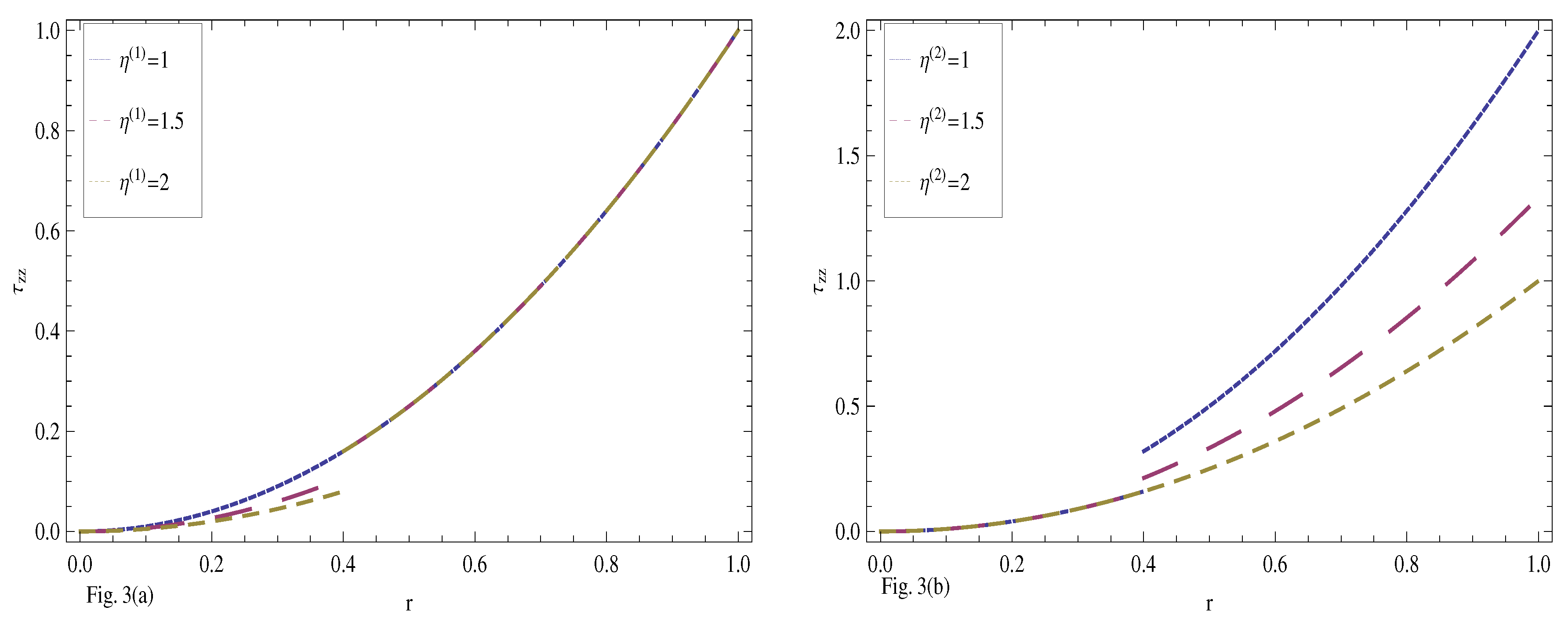
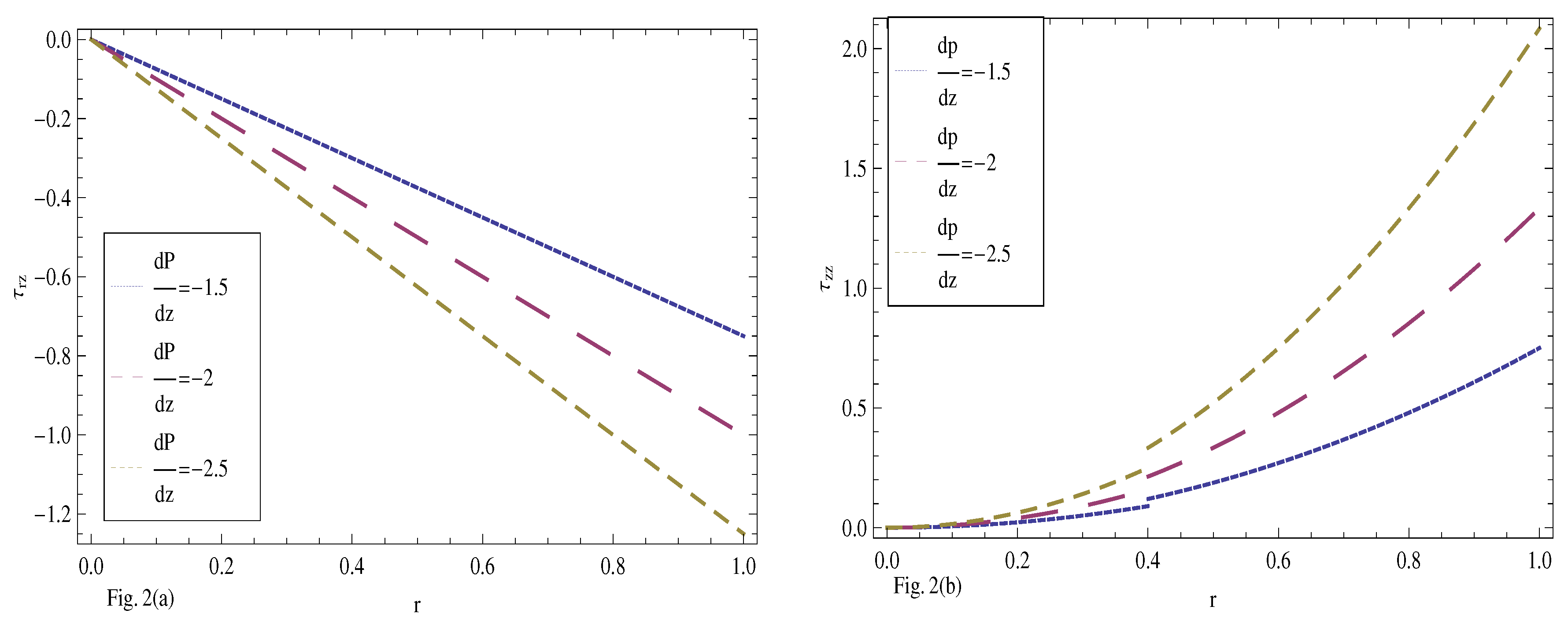
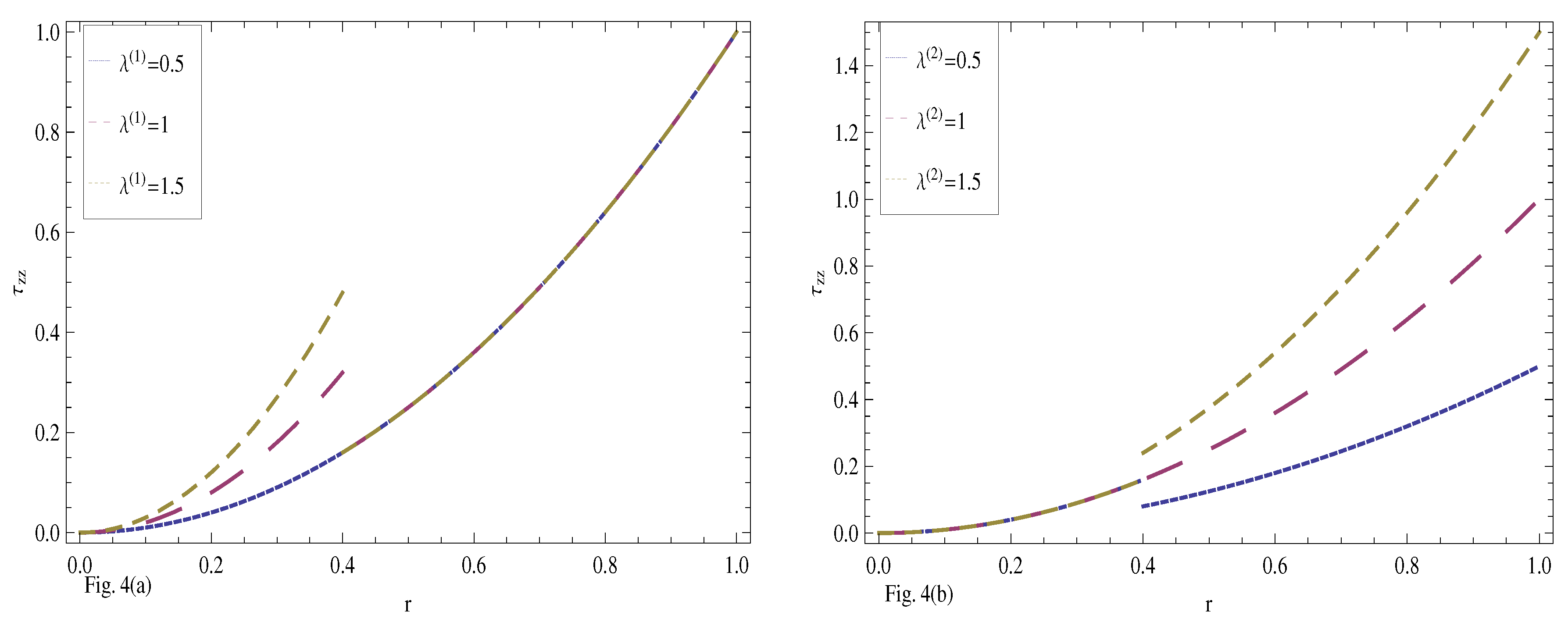
5.1. Stresses

The concentric heat transfer flow of two immiscible PTT fluids in a pipe is modeled and studied. Mathematical modeling in the geometry under consideration together with the physical assumptions develops the ordinary differential equations which helped in calculating the expressions for stress distributions, velocity profiles, and temperature distributions. In this section, we have to check the behavior of involved parameters on stress distributions, velocity profiles and temperature distributions.

Figure 2 a shows the effect of pressure gradient on the shear stresses given in Equation (36). The curves shown in Figure 2a are plotted by fixing $\xi =0.4,{\eta }^{(1)}=1,{\eta }^{(2)}=2,{\lambda }^{(1)}=0.5$, and ${\lambda }^{(2)}=1$, while the values for pressure gradient ${\displaystyle \frac{dp}{dz}}$ are varied to give three different curves. The graph shows that shear stresses vary linearly with distance from the axis of the pipe and that they are independent of the material constants of any of the fluids.

Figure 2. The effect of pressure gradient on the (a) shear stresses (b) normal stresses when $\xi =0.4$.

In Figure 2b, the effect of pressure gradient on normal stresses given in Equation (37) is shown by fixing ${\eta }^{(2)}=1.5$, while the other constants are fixed as before. The three curves in Figure 2b show that the relation of normal stress ${\tau }_{zz}$ with r is not linear in nature and the irregularities at the interface of the two fluids show that the normal stresses depend on the material constants.

The graphs in Figure 3a are plotted to show the effect of the viscosity coefficient ${\eta }^{(1)}$ on the normal stresses of the two fluids. The curves are plotted by keeping $\xi =0.4,{\eta }^{(2)}=2,{\lambda }^{(1)}=0.5,{\lambda }^{(2)}=1$ and ${\displaystyle \frac{dp}{dz}}=-2.$ The three values of ${\eta }^{(1)}$ yield three different curves for fluid in the core but the curves overlap for the fluid in the outer layer. This is because ${\tau }_{zz}^{(1)}$ depends on ${\eta }^{(1)}$ but not on ${\eta }^{(2)}$. Similarly, in case of graphs shown in Figure 3b, fixing ${\eta }^{(1)}=1$ and varying ${\eta }^{(2)}$ gives three different curves for fluid (2) but the curves overlap in the region of fluid (1).

Figure 3. The effect of (a) viscosity coefficient ${\eta }^{(1)}$, (b) viscosity coefficient ${\eta }^{(2)}$, on the normal stresses of the two fluids.

In Figure 4a,b, the effects of relaxation times ${\lambda }^{(1)}$ and ${\lambda }^{(2)}$ on the normal stresses of the two fluids are shown, respectively. The normal stress of fluid (1) depend on ${\lambda }^{(1)}$ and not on ${\lambda }^{(2)}$ while the fluid (2) depends on ${\lambda }^{(2)}$ and not on ${\lambda }^{(1)}$. In Figure 4a, the values are fixed as $\xi =0.4,{\eta }^{(1)}=1,{\eta }^{(2)}=2,$ ${\displaystyle \frac{dp}{dz}}=-2$ and ${\lambda }^{(2)}=1$, and variation of ${\lambda }^{(1)}$ is monitored. The graphs in Figure 4b show the effect of ${\lambda }^{(2)}$ while keeping ${\lambda }^{(1)}=0.5$. Values of the remaining parameters are taken to be the same as those for Figure 4a.

Figure 4. The effect on the normal stresses of the two fluids of (a) ${\lambda }^{(1)}$ and (b) ${\lambda }^{(2)}$.

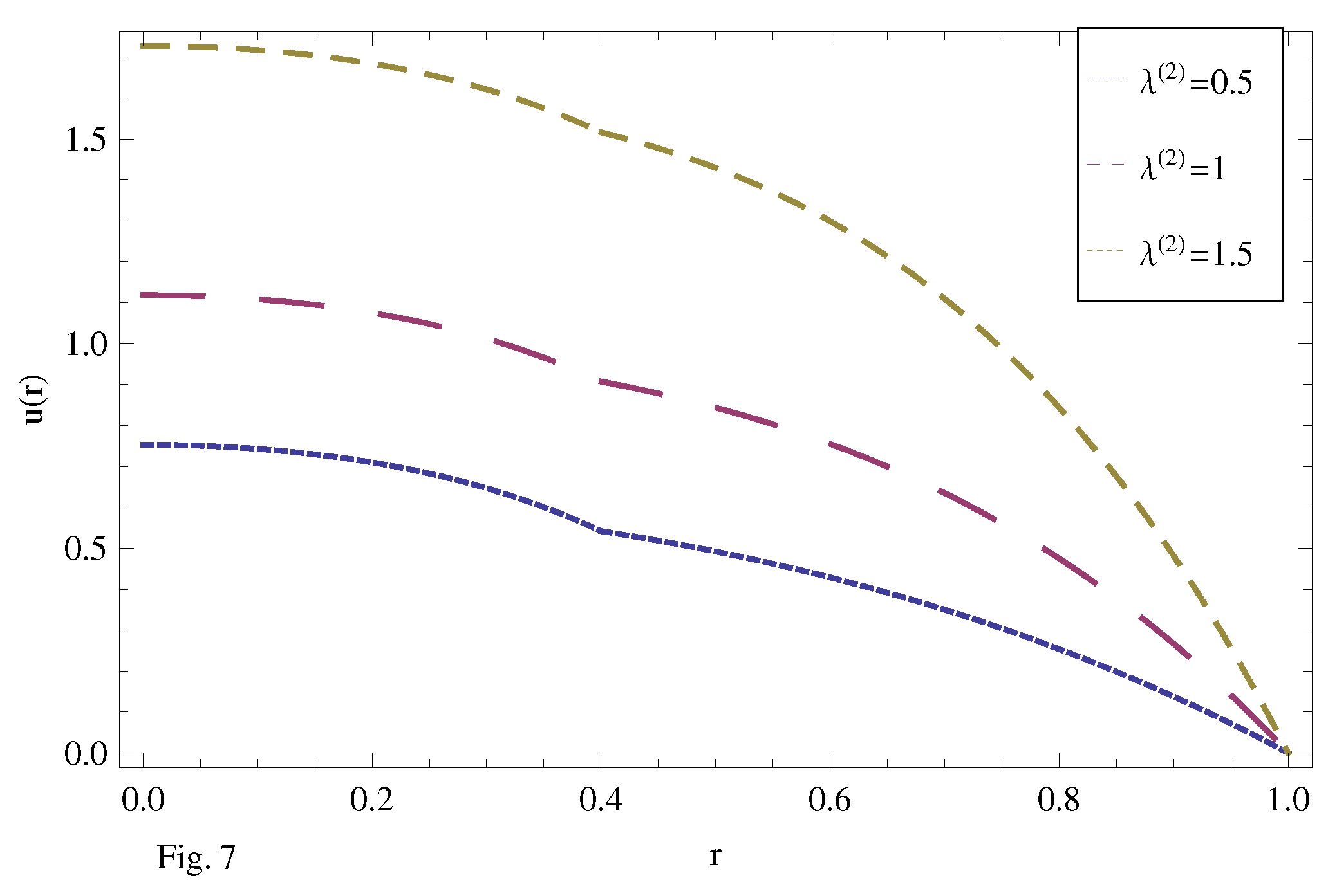
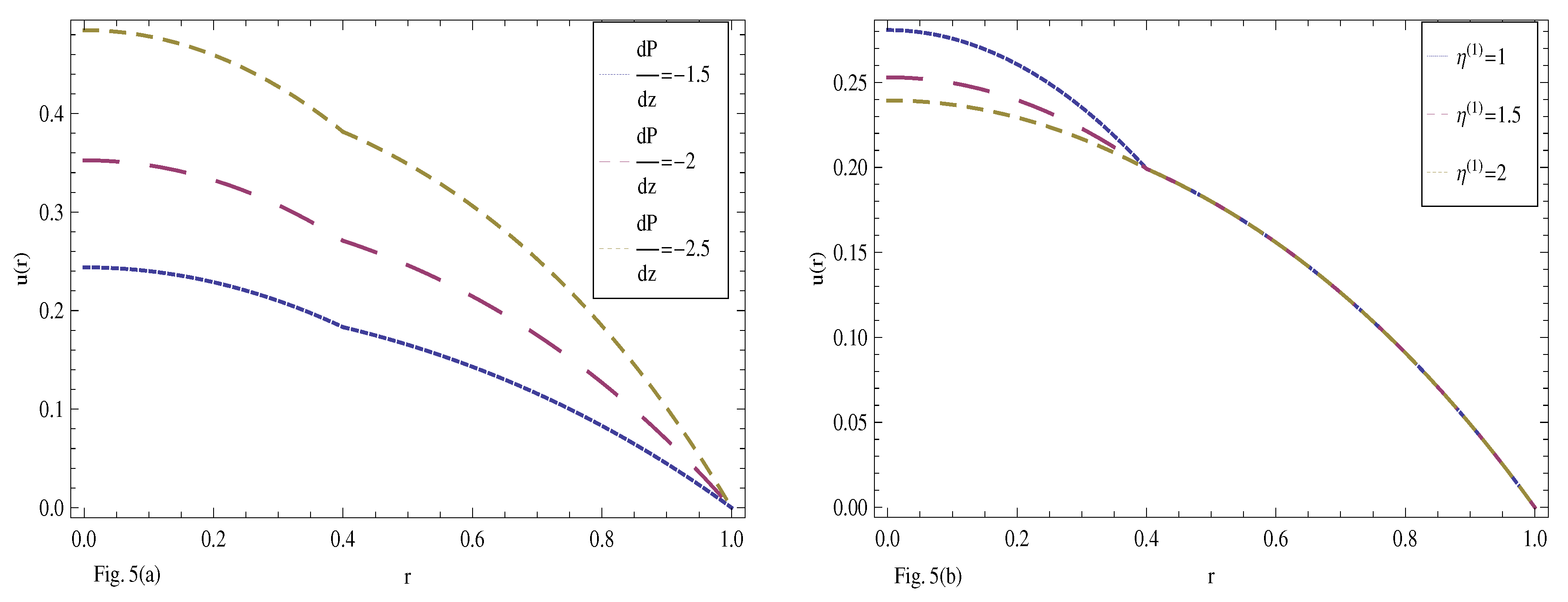
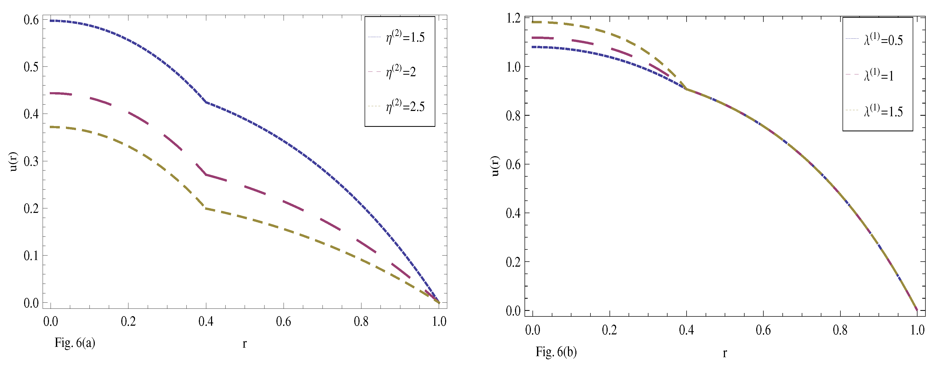
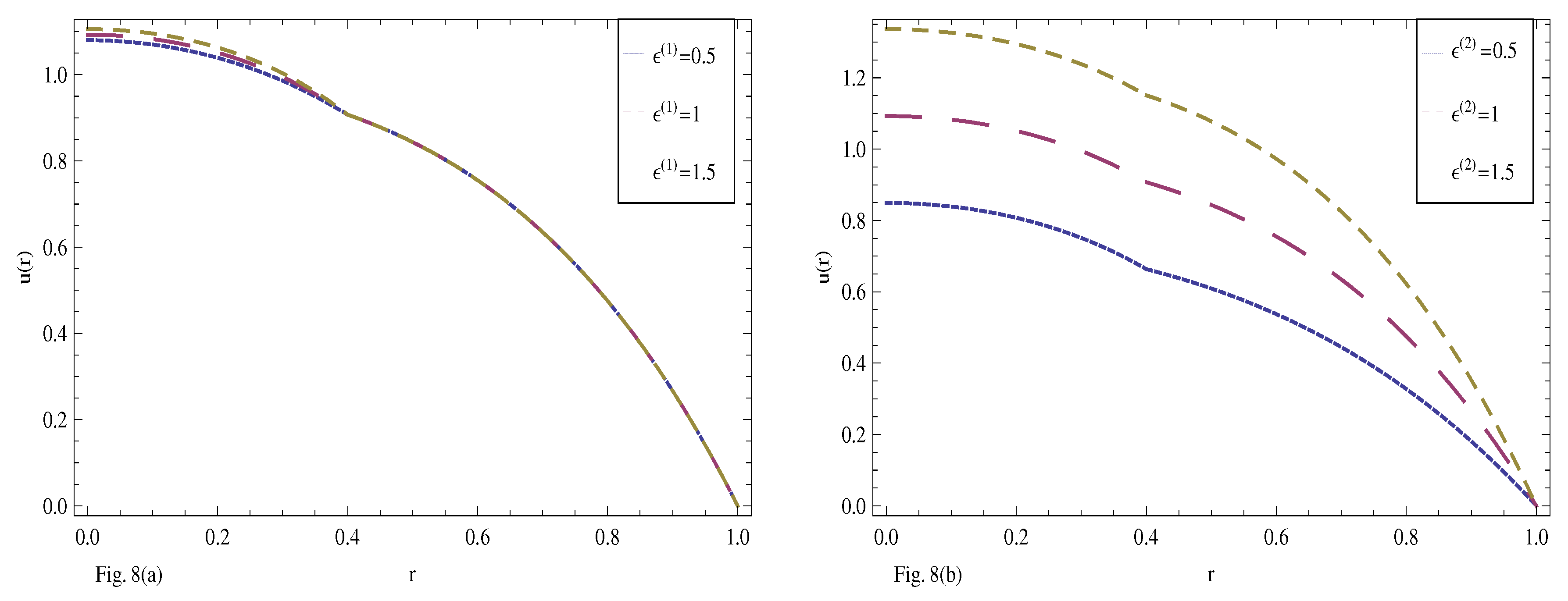
5.2. Velocities

Figure 5, Figure 6, Figure 7 and Figure 8, show the graphs in which the effects of various parameters on the velocities of the two fluids given by Equations (44) and (45) are studied.

Figure 5. The effect of (a) ${\displaystyle \frac{dp}{dz}}$ and (b) ${\eta }^{(1)}$ on the velocities of the two fluids.

Figure 6. The effect of (a) ${\eta }^{(2)}$ and (b) ${\lambda }^{(1)}$ on the velocities of the two fluids.

Figure 7. Effect of ${\lambda }^{(2)}$ on the velocities of the two fluids.

Figure 8. Effect of (a) ${ϵ}^{(1)}$ and (b) ${ϵ}^{(2)}$ on the velocities of the two fluids.

In Figure 5a, the graphs are plotted by fixing $\xi =0.4,{\eta }^{(1)}=1,{\eta }^{(2)}=2,{ϵ}^{(1)}=0.5,$ ${ϵ}^{(2)}=1,$ ${\lambda }^{(1)}=0.5$, and ${\lambda }^{(2)}=1$ and the three curves shown are obtained for different values of the pressure gradient ${\displaystyle \frac{dp}{dz}}$. The graph clearly indicates the continuity of velocities at the interface of the fluids. It is observed that with increasing values of pressure gradient the velocity profiles of the fluids also increase.

Figure 5b demonstrates the effect that is observed on the velocities of the fluids when the values of ${\eta }^{(1)}$ are varied. The values that are kept fixed while plotting the graphs are $\xi =0.4,{\displaystyle \frac{dp}{dz}}=-2,$ ${\eta }^{(2)}=2.5,$ ${ϵ}^{(1)}=0.5,{ϵ}^{(2)}=1,{\lambda }^{(1)}=0.5$, and ${\lambda }^{(2)}=1$. It is observed that the three curves in Figure 5b overlap in the region where fluid (2) is flowing. It is also clearly indicated by Equation (44) that the expression $u^{(2)}$ does not involve the coefficient of viscosity ${\eta }^{(1)}$ of fluid (1) in it and therefore the values of ${\eta }^{(1)}$ does not affect velocity of the fluid (2). However, since both the expressions (44) and (45) involve the parameter ${\eta }^{(2)}$, the velocities of both the fluids are affected by varying the values of the parameters as those used for Figure 5b but fixing ${\eta }^{(1)}=0.5$ this time and varying the value of ${\eta }^{(2)}$ as shown in Figure 6a. It is observed that with increasing values of ${\eta }^{(2)}$ the velocity profiles of the fluids seem to be slow down.

In Figure 6b, the effect of ${\lambda }^{(1)}$ on the velocities of the two fluids is studied for the fixed values of $\xi =0.4,{\displaystyle \frac{dp}{dz}}=-2,{\eta }^{(1)}=0.5,{\eta }^{(2)}=1,{ϵ}^{(1)}=0.5,{ϵ}^{(2)}=1$, and ${\lambda }^{(2)}=1$. This Figure also indicates that variation in the value of ${\lambda }^{(1)}$ does not play any role in the velocity of the fluid (2). Figure 7 is plotted with same choice of values of parameters but the value of ${\lambda }^{(1)}$ is fixed to be 1 and ${\lambda }^{(2)}$ is kept variable.

Figure 8a,b, demonstrate the influence of the elongation parameters ${ϵ}^{(1)}$ and ${ϵ}^{(2)}$, respectively, on velocities of the two fluids. Both the Figure 8a,b, are plotted for the fixed values of $\xi =0.4,$ ${\displaystyle \frac{dp}{dz}}=-2,$ ${\eta }^{(1)}=0.5,{\eta }^{(2)}=1,{\lambda }^{(1)}=0.5$, and ${\lambda }^{(2)}=1$. For Figure 8a, ${ϵ}^{(2)}=1$, and for Figure 8b, ${ϵ}^{(1)}=1$ are taken.

It is also noted that the maximum velocity exists in the core of the pipe and this phenomenon has important application in transportation and pumping of immiscible fluids.

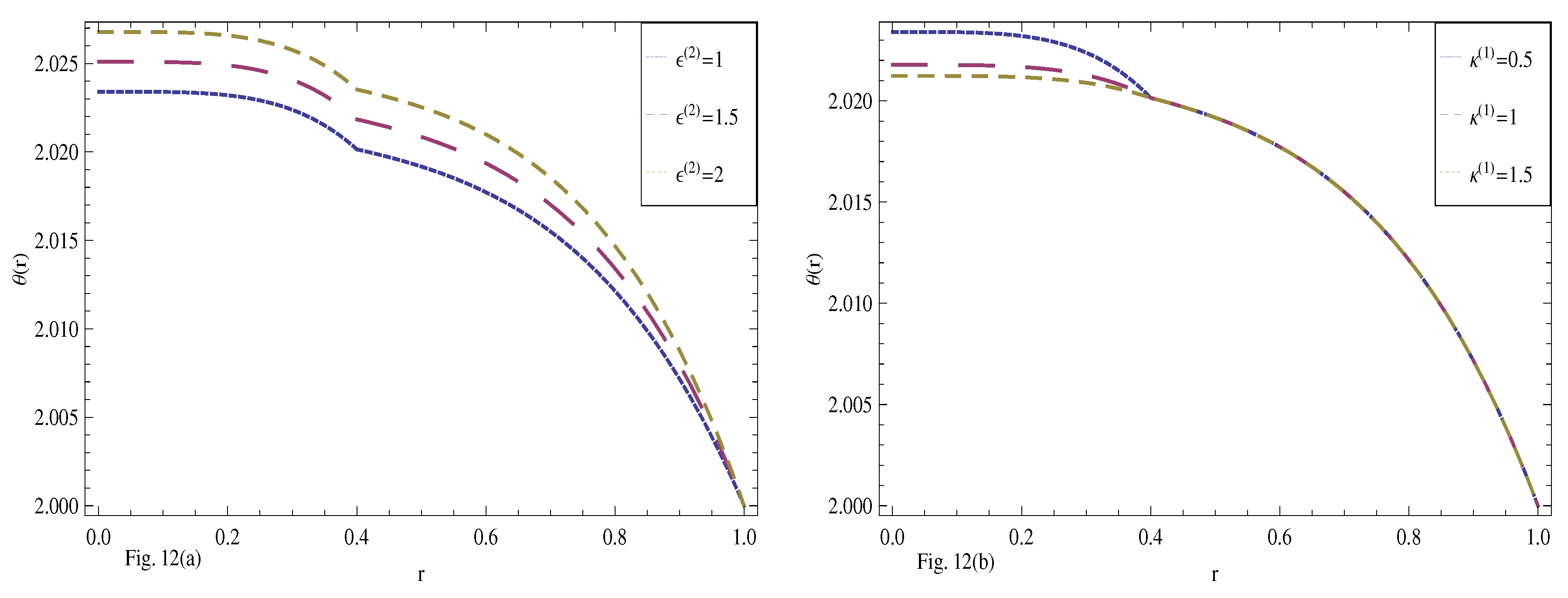
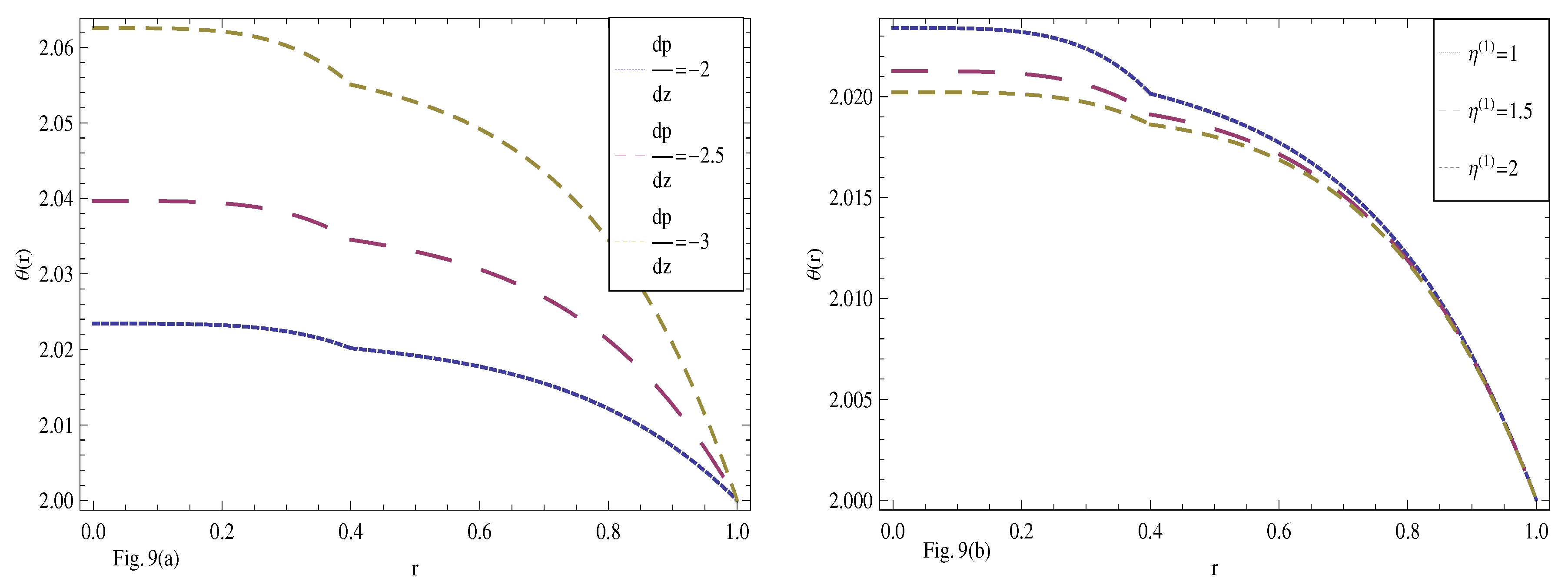
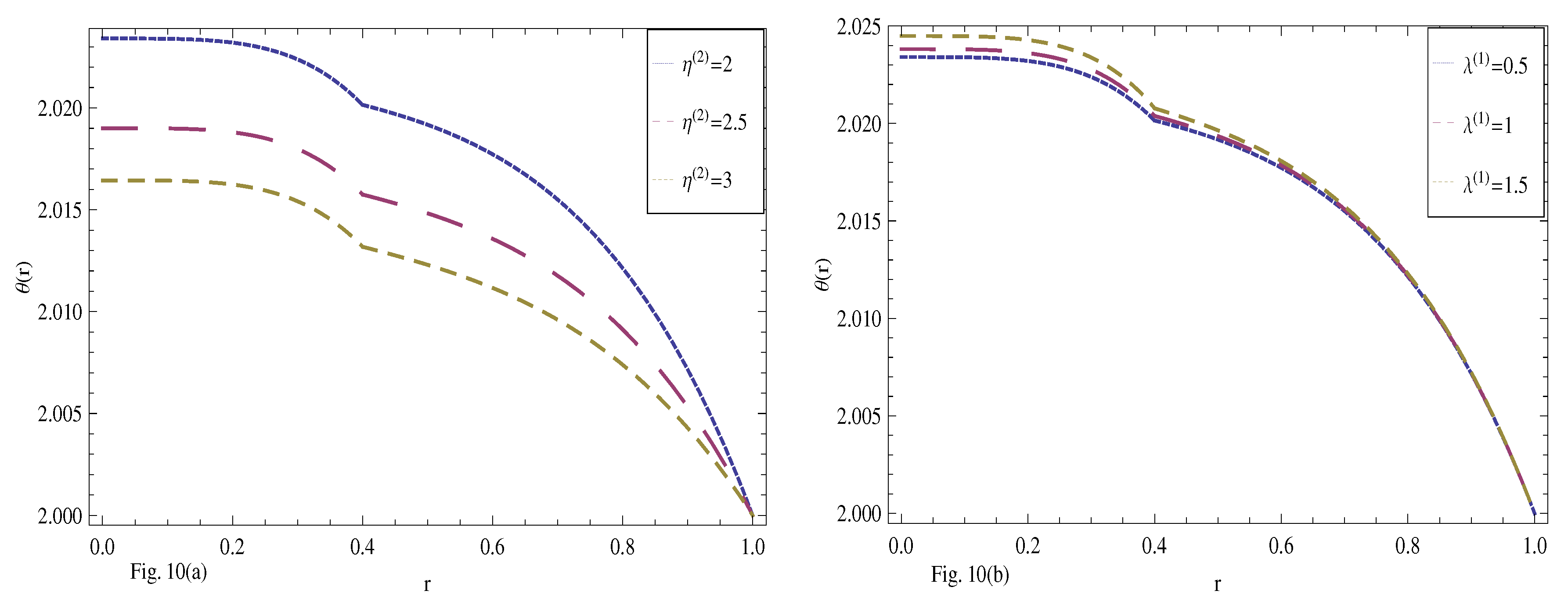
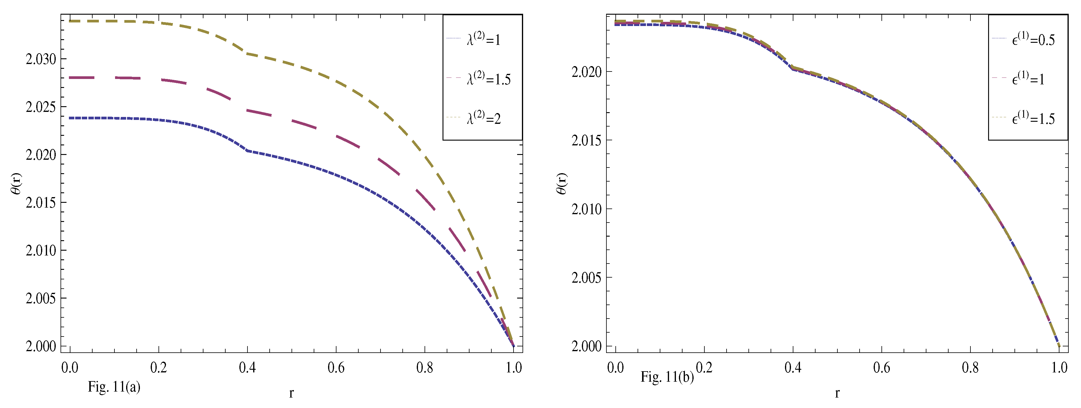
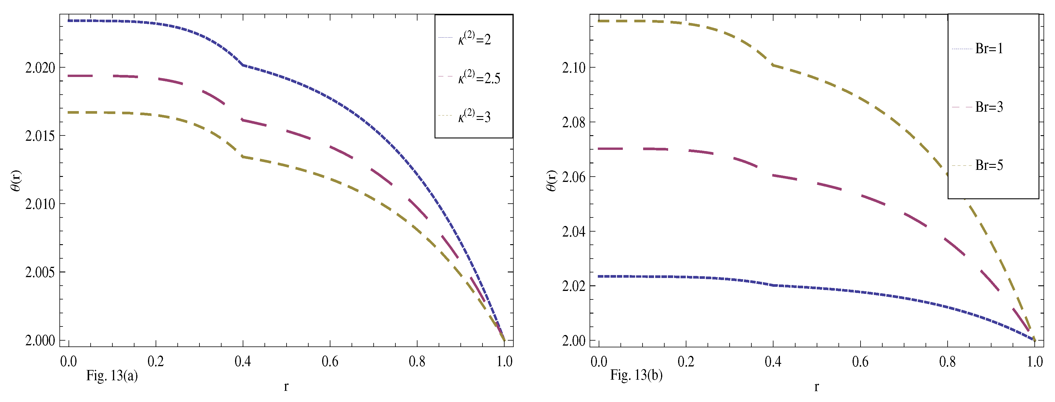
5.3. Temperatures

Figure 9, Figure 10, Figure 11, Figure 12 and Figure 13 present graphs that are plotted for temperature distribution of the two fluids given by expressions (60) and (62).

Figure 9. Effect of (a) ${\displaystyle \frac{dp}{dz}}$ and (b) ${\eta }^{(1)}$ on the temperatures of the two fluids.

Figure 10. Effect of (a) ${\eta }^{(2)}$ and (b) ${\lambda }^{(1)}$ on the temperatures of the two fluids.

Figure 11. Effect of (a) ${\lambda }^{(2)}$ and (b) ${ϵ}^{(1)}$ on the temperatures of the two fluids.

Figure 12. Variation of (a) ${ϵ}^{(2)}$ and (b) ${\kappa }^{(1)}$ on the temperatures of the two fluids.

Figure 13. Variation of (a) ${\kappa }^{(2)}$ and (b) $Br$ on the temperatures of the two fluids.

Figure 9a shows a graph in which dependence of the temperatures on pressure gradient ${\displaystyle \frac{dp}{dz}}$ is observed. The graph in Figure 9a is plotted for the fixed values of ${\mathsf{\Theta }}_o=2$, $\xi =0.4$, ${\eta }^{(1)}=1$, ${\eta }^{(2)}=2$, ${ϵ}^{(1)}=0.5$, ${ϵ}^{(2)}=1$, ${\lambda }^{(1)}=0.5$, ${\lambda }^{(2)}=1$, $Br=1$, ${\kappa }^{(1)}=0.5$ and ${\kappa }^{(2)}=2$. This Figure clearly shows that temperatures of both the fluids vary with varying values of pressure gradient.

In Figure 9b, the effect of ${\eta }^{(1)}$ on fluid temperatures is studied. The fixed values of the parameters while plotting the graph in Figure 9b are taken to be ${\mathsf{\Theta }}_o=2$, $\xi =0.4$, ${\displaystyle \frac{dp}{dz}}=-2$, ${\eta }^{(2)}=2$, ${ϵ}^{(1)}=0.5$, ${ϵ}^{(2)}=1$, ${\lambda }^{(1)}=0.5$, ${\lambda }^{(2)}=1$, $Br=1$, ${\kappa }^{(1)}=0.5$ and ${\kappa }^{(2)}=2$. Three different values of ${\eta }^{(1)}$ yield three different curves showing that the value of ${\eta }^{(1)}$ affects temperatures of both the fluids. However, Figure 10a shows that the effect of ${\eta }^{(2)}$ on the temperature profiles is much more significant than that of ${\eta }^{(1)}$. For the graph in Figure 10a, ${\eta }^{(1)}=1$ and the value of ${\eta }^{(2)}$ is varied to give three different curves.

The graphs in Figure 10b and Figure 11a show that relaxation times ${\lambda }^{(1)}$ and ${\lambda }^{(2)}$ of both the fluids affect the temperatures. The parameters are assigned the values ${\mathsf{\Theta }}_o=2$, $\xi =0.4$, ${\displaystyle \frac{dp}{dz}}=-2$, ${\eta }^{(1)}=2$, ${\eta }^{(2)}=2$, ${ϵ}^{(1)}=0.5$, ${ϵ}^{(2)}=1$, $Br=1$, ${\kappa }^{(1)}=0.5$ and ${\kappa }^{(2)}=2$ while plotting the graphs. For the graph in Figure 10b, the value of ${\lambda }^{(2)}=1$ and for the one in Figure 11a, the value of ${\lambda }^{(1)}=1$.

Figure 11b and Figure 12a illustrate the effect of the parameters ${ϵ}^{(1)}$ and ${ϵ}^{(2)}$ on temperatures of the two fluids. These graphs are plotted for the fixed values of ${\mathsf{\Theta }}_o=2$, $\xi =0.4$, ${\displaystyle \frac{dp}{dz}}=-2$, ${\eta }^{(1)}=1$, ${\eta }^{(2)}=2$, ${\lambda }^{(1)}=0.5$, ${\lambda }^{(2)}=1$, $Br=1$, ${\kappa }^{(1)}=0.5$ and ${\kappa }^{(2)}=2$. ${ϵ}^{(2)}=1$ and ${ϵ}^{(1)}=0.5$ in Figure 11b and Figure 12a, respectively.

Finally, in the graphs shown in Figure 12b and Figure 13, the effects of thermal conductivities ${\kappa }^{(1)}$ and ${\kappa }^{(2)}$ of the two fluids on their temperatures are studied. The graph in Figure 12b is plotted for the fixed values of ${\mathsf{\Theta }}_o=2$, $\xi =0.4$, ${\displaystyle \frac{dp}{dz}}=-2$, ${\eta }^{(1)}=1$, ${\eta }^{(2)}=2$, ${ϵ}^{(1)}=0.5$, ${ϵ}^{(2)}=1$, $Br=1$, ${\lambda }^{(1)}=0.5$ and ${\lambda }^{(2)}=1$. ${\kappa }^{(2)}=2$ for Figure 12b. As is evident from relation (48), the thermal conductivity ${\kappa }^{(1)}$ does not affect the temperature ${\mathsf{\Theta }}^{(2)}$ of the fluid (2). Therefore, the three curves for three different values of ${\kappa }^{(1)}$ in Figure 12b overlap to give a single curve for temperature of fluid (2). However, variation in the value of ${\kappa }^{(1)}$ does affect ${\mathsf{\Theta }}^{(1)}$. Since both the expressions (48) and (50) involve the parameter ${\kappa }^{(2)}$, we obtain three different curves for temperatures of both the fluids when ${\kappa }^{(2)}$ is assigned three different values and ${\kappa }^{(1)}=0.5$. The last Figure 13b shows the effect of Brinkman number $Br$ on the temperature distribution, it is noted that the increase in the values of $Br$, increases the temperature distribution in the fluid layers.

5.4. Application—Optimal Value of $\xi$ for Maximal Flow Rate

We have observed, using graphs, that the flow parameters, both viscosities as well as non-Newtonian parameters affect velocities, stress distributions and temperature profiles. In addition to this, we would like to emphasize that the solutions presented here can be of useful importance in many practical situations. As an example, we consider the case where there is a highly viscous fluid flowing through a pipe, and a relatively less viscous fluid is introduced along the boundary of the pipe to help more efficient and faster flow of the inner fluid. Using relations (54) and (55), we can find the optimal value of $\xi$ in order to maximize the flow rate of inner fluid. For instance, using the set of parameter values

$${\eta }^{(1)}=2,{\eta }^{(2)}=1,{ϵ}^{(1)}=0.25,{ϵ}^{(2)}=0.5,{\lambda }^{(1)}=2,{\lambda }^{(2)}=1,\frac{dp}{dz}=-2,$$

(73)

in a computer algebra system in order to maximize $Q^{(1)}$, we find that the optimal value of $\xi$ is $0.8056$. With this value of $\xi$ in hand, we can set the thickness of the extra outer fluid layer that we introduced in order to obtain maximal flow rate of the inner fluid. The analysis of this result becomes significant especially when there is limited amount of pressure gradient (or fluid pumping efficiency) available to drive the flow.

6. Conclusions

The concentric non-isothermal flow of two immiscible PTT fluids in a pipe is modeled and studied. Mathematical modeling in the geometry under consideration together with the physical assumptions develops the ordinary differential equations which helped in calculating the expressions for stress distributions, velocity profiles, and temperature distributions. The existing results for two immiscible viscous fluids have been recovered from the obtained solutions by neglecting PTT fluid material parameters. The effects of the involved parameters on stress distributions, velocity profiles, and temperature distributions are discussed with the help of graphs.

It is observed that:

• Shear stresses vary linearly and independently of the material constants.
• Normal stresses are not linear in nature and depend on the material constants.
• Continuity of velocities exists at interface.
• The results for Newtonian fluids can be deduced by substituting material parameters ${\lambda }^{(1)}={\lambda }^{(2)}=0$.
• The expression for velocities when one of the two fluids is Newtonian in nature can be deduced by substituting the $\lambda$ corresponding to that fluid equal to zero.
• Velocities play basic roles in the transportation of the fluids; graphical representations show that fluid velocities can be controlled with the proper choice of the involved parameters.
• The approach for solving the problem is also applicable to the flow of a finite number of layers, in which case, the continuity of velocities at interfaces results in one fluid affecting the flow of its adjacent inner layer.
• The number of fluid layers does not affect the existence of a unique velocity maximum, which is always in the innermost fluid layer, and this observation has great impact on the transportation and pumping of immiscible fluids.

References

- Malashetty, M.S.; Umavathi, J.C. Two-phase magnetohydrodynamic flow and heat transfer in an inclined channel. Int. J. Multiph. Flow 1997, 23, 545–560. [Google Scholar] [CrossRef]
- Elmaboud, Y.A.; Abdelsalam, S.I.; Mekheimer, K.S.; Vafai, K. Electromagnetic flow for two-layer immiscible fluids. Eng. Sci. Technol. Int. J. 2018. [Google Scholar] [CrossRef]
- Packham, B.A.; Shail, R. Stratified laminar flow of two immiscible fluids. Math. Proc. Camb. Philos. Soc. 1971, 69, 443–448. [Google Scholar] [CrossRef]
- Brauner, N. Two-phase liquid-liquid annular flow. Int. J. Multiph. Flow 1991, 17, 59–76. [Google Scholar] [CrossRef]
- Lohrasbi, J.; Sahai, V. Magnetohydrodynamic heat transfer in two-phase flow between parallel plates. Appl. Sci. Res. 1988, 45, 53–66. [Google Scholar] [CrossRef]
- Malashetty, M.S.; Leela, V. Magnetohydrodynamic heat transfer in two phase flow. Int. J. Eng. Sci. 1992, 30, 371–377. [Google Scholar] [CrossRef]
- Shail, R. On laminar two-phase flows in Magnetohydrodynamics. Int. J. Eng. Sci. 1973, 11, 1103–1108. [Google Scholar] [CrossRef]
- Leib, T.M.; Hasson, D. Heat transfer in vertical annular laminar flow of two immiscible liquids. Int. J. Multiph. Flow 1977, 3, 533–549. [Google Scholar] [CrossRef]
- Siddiqui, A.M.; Azim, Q.A.; Rana, M.A. On exact solutions of concentric n-layer flows of viscous fluids in a pipe. Nonlinear Sci. Lett. A 2010, 1, 67–76. [Google Scholar]
- Cruz, D.O.A.; Pinho, F.T. Analysis of isothermal flow of a Phan-Thien-Tanner fluid in a simplified model of a single- screw-extruder. J. Non-Newton. Fluid Mech. 2012, 167–168, 95–105. [Google Scholar] [CrossRef]
- Tanner, R.I. Engineering Rheology; OUP: Oxford, UK, 2000; Volume 52. [Google Scholar]
© 2019 by the authors. Licensee MDPI, Basel, Switzerland. This article is an open access article distributed under the terms and conditions of the Creative Commons Attribution (CC BY) license (http://creativecommons.org/licenses/by/4.0/).
Share and Cite
Siddiqui, A.M.; Zeb, M.; Haroon, T.; Azim, Q.-u.-A. Exact Solution for the Heat Transfer of Two Immiscible PTT Fluids Flowing in Concentric Layers through a Pipe. Mathematics 2019, 7, 81. https://doi.org/10.3390/math7010081
Siddiqui AM, Zeb M, Haroon T, Azim Q-u-A. Exact Solution for the Heat Transfer of Two Immiscible PTT Fluids Flowing in Concentric Layers through a Pipe. Mathematics. 2019; 7(1):81. https://doi.org/10.3390/math7010081
Chicago/Turabian StyleSiddiqui, Abdul Majeed, Muhammad Zeb, Tahira Haroon, and Qurat-ul-Ain Azim. 2019. "Exact Solution for the Heat Transfer of Two Immiscible PTT Fluids Flowing in Concentric Layers through a Pipe" Mathematics 7, no. 1: 81. https://doi.org/10.3390/math7010081
APA StyleSiddiqui, A. M., Zeb, M., Haroon, T., & Azim, Q.-u.-A. (2019). Exact Solution for the Heat Transfer of Two Immiscible PTT Fluids Flowing in Concentric Layers through a Pipe. Mathematics, 7(1), 81. https://doi.org/10.3390/math7010081