New Approach for Fractional Order Derivatives: Fundamentals and Analytic Properties

Abstract

The rate of change of any function versus its independent variables was defined as a derivative. The fundamentals of the derivative concept were constructed by Newton and l’Hôpital. The followers of Newton and l’Hôpital defined fractional order derivative concepts. We express the derivative defined by Newton and l’Hôpital as an ordinary derivative, and there are also fractional order derivatives. So, the derivative concept was handled in this paper, and a new definition for derivative based on indefinite limit and l’Hôpital’s rule was expressed. This new approach illustrated that a derivative operator may be non-linear. Based on this idea, the asymptotic behaviors of functions were analyzed and it was observed that the rates of changes of any function attain maximum value at inflection points in the positive direction and minimum value (negative) at inflection points in the negative direction. This case brought out the fact that the derivative operator does not have to be linear; it may be non-linear. Another important result of this paper is the relationships between complex numbers and derivative concepts, since both concepts have directions and magnitudes.

1. Introduction

The asymptotic behaviors of functions can be analyzed by velocities or rates of change in functions, while very small changes occur in the independent variables. The concept of rate of change in any function versus change in the independent variables was defined as a derivative, and this concept attracted many scientists and mathematicians such as Newton, l’Hôpital, Leibniz, Abel, Euler, Riemann, etc.

Isaac Newton defined the fundamentals of classical mechanics and this study contains rates of changes of functions [1]. He collected his works in Philosophiæ Naturalis Principia Mathematica, a book that includes geometrical proofs, gravitational force law, and attraction of bodies [1]. He was the first scientist who concerned himself with the concept of derivatives/fluxions. On the other hand, Newton tried to determine the change in length of distance in terms of the velocity of bodies, and the change in velocity of bodies in terms of acceleration. L’Hôpital was a follower of Newton in that he defined the concept of a derivative and generalized this concept. There are other mathematicians who dealt with the concepts of derivatives/fluxions.

The first important and detailed work in differential calculus and differential geometry was done by l’Hôpital [2,3]. L’Hôpital generalized the ideas of Newton through variations on calculus. Leibniz is another scientist who expounded on differential calculus and infinitesimal calculus [4]; he mastered the mathematics of his day and developed his own calculus over the short span of a few years [4]. Newton, l’Hôpital, and Leibniz are not the only mathematicians who dealt with variations of calculus. Some mathematicians tried to explain the ratio between the two displacements of at least two variables [5], since it is important for analyzing the asymptotic behaviors of functions.

The asymptotic behaviors of functions can be regarded as the rates of displacements of functions versus rates of displacement of independent variables—in other words, the rates of movement of functions. The term fluxion indicates motion and the idea of the fluxional calculus developed from the concept that a geometrical magnitude was the result of continuous motion of a point, line, or plane [6]. This motion, speaking of plane curves, could be considered in reference to coordinate axes as the result of two motions, one in the direction of the X-axis and the other in the direction of the Y-axis [6]. The velocity of the X-component and the Y-component were called “fluxions” by Newton [1,6]. The velocity of a point is represented by an equation involving the fluxions x and y [6].

The problems of variation of calculus are attractive to mathematicians and there are several familiar mathematicians who focused their attention on these problems such as Newton, l’Hôpital, Leibniz, Euler, Abel, Caputo, Riemann, Grünwald, Miller, Ross, et al. [7,8,9,10,11].

The problems of variation of calculus and infinitesimal calculus are not solved completely, and there are still open problems in fractional variation of calculus. There are a lot of studies about the fractional variations of calculus [11,12,13,14,15,16,17,18,19,20,21,22]. Euler, Caputo, Riemann, Abel, et al. dealt with fractional variations of calculus and fractional order calculus and systems. Karci defined the fractional order derivative concept in a different way by using indefinite limits and the l’Hôpital rule [23,24,25].

Some popular fractional order derivative methods, such as Euler, Caputo, and Riemann-Liouville, can be summarized as follows.

The Euler method is $\frac{d^n{x}^m}{d{x}^n}=\frac{\Gamma (m+1)}{\Gamma (m-n+1)}{x}^{m-n}$ and its deficiencies can be illustrated for constant and identity functions. Assume that f(x) = cx⁰ where c is a constant and $c\in R$. Assume that n = 1 and $\mathsf{\alpha }=\frac{1}{4}$ and:

$$\frac{d^n{x}^m}{d{x}^n}=\frac{\Gamma (m+1)}{\Gamma (m-n+1)}{x}^{m-n}=\frac{d^{\frac{1}{4}}{x}^0}{d{x}^{\frac{1}{4}}}=\frac{\Gamma \left(\frac{5}{4}\right)}{\Gamma \left(\frac{3}{4}\right)}c{x}^{-\frac{1}{4}}$$

The derivative of any constant function is always zero; however, the result of fractional order derivative with respect to the Euler method is different from zero. Assume that f(x) = x, n = 1 and $\mathsf{\alpha }=\frac{2}{3}$.

$$\frac{d^{\frac{2}{3}}{x}^1}{d{x}^{\frac{2}{3}}}=\frac{\Gamma (1+1)}{\Gamma \left(1-\frac{2}{3}+1\right)}{x}^{1-\frac{2}{3}}=\frac{\Gamma (2)}{\Gamma \left(\frac{4}{3}\right)}{x}^{\frac{1}{3}}\ne 1$$

The Riemann-Liouville method is for function f(t) ${}_{a}D_t^{\mathsf{\alpha }}f(t)=\frac{1}{\Gamma \left(n-\mathsf{\alpha }\right)}{\left(\frac{d}{dt}\right)}^n{\displaystyle \underset{a}{\overset{t}{\int }}\frac{f(v)dv}{{(t-v)}^{\mathsf{\alpha }-n+1}}}$. The fractional order derivative also can be applied to constant and identity functions with respect to the Riemann-Liouville method.

Assuming that f(x) = cx⁰, $c\in R$, n = 1 and $\mathsf{\alpha }=\frac{2}{3}$,

$${}_{a}D_t^{\mathsf{\alpha }}f(t)=\frac{1}{\Gamma \left(n-\mathsf{\alpha }\right)}{\left(\frac{d}{dt}\right)}^n{\displaystyle \underset{a}{\overset{t}{\int }}\frac{f(v)dv}{{(t-v)}^{\mathsf{\alpha }-n+1}}}={}_{a}D_t^{\frac{2}{3}}f(t)=\frac{1}{\Gamma \left(\frac{1}{3}\right)}\frac{d}{dt}{\displaystyle \underset{a}{\overset{t}{\int }}\frac{cdv}{{(t-v)}^{\frac{2}{3}}}}=\frac{c}{\Gamma \left(\frac{1}{3}\right)}\left(-\frac{1}{{(t-a)}^{\frac{2}{3}}}\right)\ne 0$$

The obtained result is inconsistent, since the result is a function of x. However, the initial function is a constant function and its derivative is zero, since there is no change in the dependent variable. The same case is valid for identity functions.

$$\begin{array}{ll}{}_{a}D_t^{\mathsf{\alpha }}f(t)& =\frac{1}{\Gamma \left(n-\mathsf{\alpha }\right)}{\left(\frac{d}{dt}\right)}^n{\displaystyle \underset{a}{\overset{t}{\int }}\frac{f(v)dv}{{(t-v)}^{\mathsf{\alpha }-n+1}}}={}_{a}D_t^{\frac{2}{3}}f(t)=\frac{1}{\Gamma \left(\frac{1}{3}\right)}\frac{d}{dt}{\displaystyle \underset{a}{\overset{t}{\int }}\frac{xdx}{{(t-x)}^{\frac{2}{3}-1+1}}}=\frac{1}{\Gamma \left(\frac{1}{3}\right)}\frac{d}{dt}{\displaystyle \underset{a}{\overset{t}{\int }}\frac{xdx}{{(t-x)}^{\frac{2}{3}}}}\\ & =\frac{1}{\Gamma \left(\frac{1}{3}\right)}\left(3a{(t-a)}^{\frac{2}{3}}+\frac{9}{4}{(t-a)}^{\frac{4}{3}}\right)\ne 1\end{array}$$

The Caputo method is ${}_a{}^{C}D_t^{\mathsf{\alpha }}f(t)=\frac{1}{\Gamma (\mathsf{\alpha }-n)}{\displaystyle \underset{a}{\overset{t}{\int }}\frac{f^{(n)}(v)dv}{{(t-v)}^{\mathsf{\alpha }+1-n}}}$. The Caputo method does not have inconsistency for constant functions; however, it has inconsistency for identity functions. Assuming that f(x) = x, n = 1 and $\mathsf{\alpha }=\frac{2}{3}$,

$${}_a{}^{C}D_t^{\mathsf{\alpha }}f(t)=\frac{1}{\Gamma (\mathsf{\alpha }-n)}{\displaystyle \underset{a}{\overset{t}{\int }}\frac{f^{(n)}(v)dv}{{(t-v)}^{\mathsf{\alpha }+1-n}}}=\frac{1}{\Gamma \left(-\frac{1}{3}\right)}{\displaystyle \underset{a}{\overset{t}{\int }}\frac{dv}{{(t-v)}^{\frac{2}{3}+1-1}}}=\frac{1}{\Gamma \left(-\frac{1}{3}\right)}\left(3{(t-a)}^{\frac{1}{3}}\right)\ne 1$$

Due to these deficiencies, there is a need for a new approach to fractional order derivatives; this paper contains such a definition and some important properties of this approach.

This paper is organized as follows. The motivation of this paper will be presented in Section 2. Section 3 illustrates the applications of rational/irrational orders of derivatives. Section 4 is the definition and details of the new approach and puts forth the analytical results of this new approach for the derivative concept. Finally, the paper is concluded in Section 5.

2. Motivation

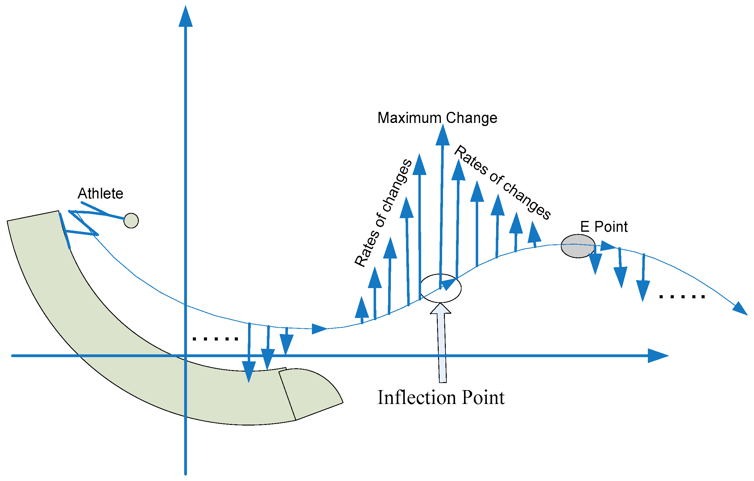
The rate of change of functions is an important concept to examine in mathematics. For this purpose, the concept of derivatives was identified, because the rate of change of the function gives detailed information about a system modeled by that function, and the nature of the problems or systems. For this purpose, an athlete’s speed may be examined on a ski-jump ramp (Figure 1). The trajectory of movement of an athlete on the ski-jump ramp can be considered as a curve. The rate of change of the athlete’s speed increases until the inflection point (Figure 1); after that point the rate of change of the athlete’s speed will decrease. So, the rate of change has its maximum at the inflection point. The rate of change of the athlete’s speed will be zero at point E (the local extremum point). The rate of change can be determined as shown in Figure 1, where it can be seen that the rate of change has magnitude and direction. The rate of change as seen in Figure 1 is directed to positive, and the situation of rates is seen in Figure 1. This concept and the relationships with complex numbers will be discussed in detail in subsequent sections of this paper.

In order to make this situation more clear and understandable, trigonometric and polynomial functions can be used. To this end, sine and cosine and two polynomial functions can be examined as examples. The rate of change can be regarded as the velocity of function change.

In order to determine the behaviors of rate of change for any function, there will be very small increments/decrements in the independent variable (these increments/decrements are equal) and the response of the dependent variable to these small increments/decrements must be examined. Assume that f(x) = sin(x) and $x\in [1,2\mathsf{\pi }]$. This closed interval can be divided into four closed intervals as follows:

$$I_1=\left[{\text{Inf}}_1,E_1\right]=\left[0,\frac{\mathsf{\pi }}{2}\right] I_2=\left[E_1,{\text{Inf}}_2\right]=\left[\frac{\mathsf{\pi }}{2},\mathsf{\pi }\right] I_3=\left[{\text{Inf}}_2,E_2\right]=\left[\mathsf{\pi },\frac{3\mathsf{\pi }}{2}\right] \text{and} I_4=\left[E_2,{\text{Inf}}_3\right]=\left[\frac{3\mathsf{\pi }}{2},2\mathsf{\pi }\right]$$

The first interval I₁ = [Inf₁, E₁] can be examined for equal-length increments/decrements in the independent variable x such as Δx₁ = Δx₂ = … = Δx_n-1 = Δx_n = Δx << 1. The first point is inflection point [Inf₁, E₁]; assume that y_inf1 = sin(x_inf1) is valid.

(a)

$x\text{inf}1\in [\text{inf}1,E1]$ and 1 ≤ i ≤ n

x_1inf1 = x_inf1 + Δx

y_1inf1 = y_inf1 + Δy_1inf1 = sin(x_inf1 + Δx)

x_2inf1 = x_1inf1 + Δx = x_inf1 + 2Δx

y_2inf1 = y_1inf1 + Δy_2inf1 = y_inf1 + Δy_1inf1 + Δy_2inf1 = sin(x_1inf1 + Δx) = sin(x_inf1 + 2Δx)

x_3inf1 = x_2inf1 + Δx = x_1inf1 + 2Δx = x_inf1 + 3Δx

y_3inf1 = y_2inf1 + Δy_3inf1 = y_1inf1 + Δy_2inf1 + Δy_3inf1 = sin(x_2inf1 + Δx) = sin(x_1inf1 + 2Δx) = sin(x_inf1 + 3Δx)

……

x_ninf1 = x_(n-1)inf1 + Δx = x_inf1 + ${\displaystyle \sum _{i=1}^n\Delta x}=x_{\text{inf}1}+n\Delta x$

$y_{n\text{inf}1}=\text{sin}\left(x_{\text{inf}1}+{\displaystyle \sum _{i=1}^n\Delta x}\right)=\text{sin}\left(x_{\text{inf}1}+n\Delta x\right)$.

At this point, the changes in the dependent variable y = f(x) are Δy_1inf1, Δy_2inf1, …, Δy_(n-1)inf1, Δy_ninf1 and inequalities for these changes are as follows: Δy_1inf1 ≥ Δy_2inf1 ≥ …. ≥ Δy_(n-1)inf1 ≥ Δy_ninf1 and |Δy_1inf1| ≥ |Δy_2inf1| ≥ …. ≥ |Δy_(n-1)inf1| ≥ |Δy_ninf1|. So, the velocities of change can be identified as follows:

$$\frac{\Delta y_{1\text{inf}1}-\Delta y_{2\text{inf}1}}{\Delta x}\ge \frac{\Delta y_{2\text{inf}1}-\Delta y_{3\text{inf}1}}{\Delta x}\ge \mathrm{....}\ge \frac{\Delta y_{(n-2)\text{inf}1}-\Delta y_{(n-1)\text{inf}1}}{\Delta x}\ge \frac{\Delta y_{(n-1)\text{inf}1}-\Delta y_{n\text{inf}1}}{\Delta x}\ge 0$$

(b)

The same argument can be made for the second closed interval $\Delta x\in I2=[E1,\text{Inf}2]$, and y = f(x) = sin(x_E1).

x_1E1 = x_E1 + Δx

y_1E1 = y_E1 + Δy_1E1 = sin(x_E1 + Δx)

x_2E1 = x_1E1 + Δx = x_E1 + 2Δx

y_2E1 = y_1E1 + Δy_2E1 = y_E1 + Δy_1E1 + Δy_2E1 = sin(x_1E1 + Δx) = sin(x_E1 + 2Δx)

x_3E1 = x_2E1 + Δx₃ = x_1E1 + 2Δx = x_E1 + 3Δx

y_3E1 = y_2E1 + Δy_3E1 = y_1E1 + Δy_2E1 + Δy_3E1 = sin(x_2E1 + Δx) = sin(x_1E1 + 2Δx) = sin(x_E1 + 3Δx)

……

x_nE1 = x_(n-1)E1 + Δx = x_E1 + ${\displaystyle \sum _{i=1}^n\Delta x}=x_{E1}+n\Delta x$

$y_{nE1}=\text{sin}\left(x_{E1}+{\displaystyle \sum _{i=1}^n\Delta x}\right)=\text{sin}\left(x_{E1}+n\Delta x\right)$.

At this point, the changes in the dependent variable y = f(x) are Δy_1E1, Δy_2E1, …, Δy_(n-1)E1, Δy_nE1 and inequalities for these changes are as follows: Δy_1E1 ≥ Δy_2E1 ≥ …. ≥ Δy_(n-1)E1 ≥ Δy_nE1 and |Δy_1E1| ≤ |Δy_2E1| ≤ … ≤ |Δy_(n-1)E1| ≤ |Δy_nE1|. So, the velocities of change can be identified as follows:

$$\frac{\Delta y_{1E1}-\Delta y_{2E1}}{\Delta x}\ge \frac{\Delta y_{2E1}-\Delta y_{3E1}}{\Delta x}\ge \mathrm{....}\ge \frac{\Delta y_{(n-2)E1}-\Delta y_{(n-1)E1}}{\Delta x}\ge \frac{\Delta y_{(n-1)E1}-\Delta y_{nE1}}{\Delta x}\ge 0$$

(c)

The same argument can be done for the second closed interval $\Delta x\in I3=[\text{Inf}2,E2]$, and y = f(x) = sin(x_inf2).

x_1inf2 = x_inf2 + Δx

y_1inf2 = y_inf2 + Δy_1inf2 = sin(x_inf2 + Δx)

x_2inf2 = x_1inf2 + Δx₂ = x_inf2 + 2Δx

y_2inf2 = y_1inf2 + Δy_2inf2 = y_inf2 + Δy_1inf2 + Δy_2inf2 = sin(x_1inf2 + Δx) = sin(x_inf2 + 2Δx)

x_3inf2 = x_2inf2 + Δx = x_1inf2 + 2Δx = x_inf2 + 3Δx

y_3inf2 = y_2inf2 + Δy_3inf2 = y_1inf2 + Δy_2inf2 + Δy_3inf2 = sin(x_2inf2 + Δx) = sin(x_1inf2 + 2Δx) = sin(x_inf2 + 3Δx)

……

x_ninf2 = x_(n-1)inf2 + Δx = x_inf2 + ${\displaystyle \sum _{i=1}^n\Delta x}=x_{\text{inf}2}+n\Delta x$

$y_{n\text{inf}2}=\text{sin}\left(x_{\text{inf}2}+{\displaystyle \sum _{i=1}^n\Delta x}\right)=\text{sin}\left(x_{\text{inf}2}+n\Delta x\right)$.

At this point, the changes in the dependent variable y = f(x) are Δy_1inf2, Δy_2inf2, …, Δy_(n-1)inf2, Δy_ninf2 and inequalities for these changes are as follows: Δy_1inf2 ≤ Δy_2inf2 ≤ … ≤ Δy_(n-1)inf2 ≤ Δy_ninf2 and |Δy_1inf2| ≥ |Δy_2inf2| ≥ … ≥ |Δy_(n-1)inf2| ≥ |Δy_ninf2|. So, the velocities of change can be identified as follows:

$$\frac{\Delta y_{1\text{inf}2}-\Delta y_{2\text{inf}2}}{\Delta x}\le \frac{\Delta y_{2\text{inf}2}-\Delta y_{3\text{inf}2}}{\Delta x}\le \mathrm{....}\le \frac{\Delta y_{(n-2)\text{inf}2}-\Delta y_{(n-1)\text{inf}2}}{\Delta x}\le \frac{\Delta y_{(n-1)\text{inf}2}-\Delta y_{n\text{inf}2}}{\Delta x}\le 0$$

(d)

The same argument can be made for the second closed interval $\Delta x\in I4=[E2,\text{Inf}2]$, and y = f(x) = sin(x_E2).

x_1E2 = x_E2 + Δx

y_1E2 = y_E2 + Δy_1E2 = sin(x_E2 + Δx)

x_2E2 = x_1E2 + Δx = x_E2 + 2Δx

y_2E2 = y_1E2 + Δy_2E2 = y_E2 + Δy_1E2 + Δy_2E2 = sin(x_1E2 + Δx) = sin(x_E2 + 2Δx)

x_3E2 = x_2E2 + Δx = x_1E2 + 2Δx = x_E2 + 3Δx

y_3E2 = y_2E2 + Δy_3E2 = y_1E2 + Δy_2E2 + Δy_3E2 = sin(x_2E2 + Δx) = sin(x_1E2 + 2Δx) = sin(x_E2 + 3Δx)

……

x_nE2 = x_(n-1)E2 + Δx = x_E2 + ${\displaystyle \sum _{i=1}^n\Delta x}=x_{E2}+n\Delta x$

$y_{nE2}=\text{sin}\left(x_{E2}+{\displaystyle \sum _{i=1}^n\Delta x}\right)=\text{sin}\left(x_{E2}+n\Delta x\right)$.

At this point, the changes in the dependent variable y = f(x) are Δy_1E2, Δy_2E2, …, Δy_(n-1)E2, Δy_nE2 and inequalities for these changes are as follows: Δy_1E2 ≥ Δy_2E2 ≥ … ≥ Δy_(n-1)E2 ≥ Δy_nE2 and |Δy_1E2| ≥ |Δy_2E2| ≥ … ≥ |Δy_(n-1)E2| ≥ |Δy_nE2|. So, the velocities of change can be identified as follows:

$$\frac{\Delta y_{1E2}-\Delta y_{2E2}}{\Delta x}\ge \frac{\Delta y_{2E2}-\Delta y_{3E2}}{\Delta x}\ge \mathrm{....}\ge \frac{\Delta y_{(n-2)E2}-\Delta y_{(n-1)E2}}{\Delta x}\ge \frac{\Delta y_{(n-1)E2}-\Delta y_{nE2}}{\Delta x}\ge 0$$

Similar arguments can be made for one period of a cosine function; this period was divided into four closed intervals as follows:

$$I_1=\left[E_1,{\text{Inf}}_1\right]=\left[0,\frac{\mathsf{\pi }}{2}\right] I_2=\left[{\text{Inf}}_1,E_2\right]=\left[\frac{\mathsf{\pi }}{2},\mathsf{\pi }\right] I_3=\left[E_2,{\text{Inf}}_2\right]=\left[\mathsf{\pi },\frac{3\mathsf{\pi }}{2}\right] \text{and} I_4=\left[{\text{Inf}}_2,E_3\right]=\left[\frac{3\mathsf{\pi }}{2},2\mathsf{\pi }\right]$$

The very small increments/decrements in independent variable x can be Δx₁ = Δx₂ = … = Δx_n-1 = Δx_n = Δx. First of all, the changes in the dependent variable y = f(x) = cos(x) can be examined for the closed interval I₁. At this point, the changes in the dependent variable y = f(x) are Δy_1E1, Δy_2E1, …, Δy_(n-1)E1, Δy_nE1 and inequalities for these changes are as follows: Δy_1E1 ≥ Δy_2E1 ≥ … ≥ Δy_(n-1)E1 ≥ Δy_nE1 and |Δy_1E1| ≤ |Δy_2E1| ≤ … ≤ |Δy_(n-1)E1| ≤ |Δy_nE1|. So, the velocities of change can be identified as follows:

$$\frac{\Delta y_{1E1}-\Delta y_{2E1}}{\Delta x}\le \frac{\Delta y_{2E1}-\Delta y_{3E1}}{\Delta x}\le \mathrm{....}\le \frac{\Delta y_{(n-2)E1}-\Delta y_{(n-1)E1}}{\Delta x}\le \frac{\Delta y_{(n-1)E1}-\Delta y_{nE1}}{\Delta x}\ge 0$$

The very small increments/decrements in independent variable x can be Δx₁ = Δx₂ = …. = Δx_n-1 = Δx_n = Δx. The changes in the dependent variable y = f(x) = cos(x) can be examined for the closed interval I₂. At this point, the changes in the dependent variable y = f(x) are Δy_1inf1, Δy_2inf1, …, Δy_(n-1)inf1, Δy_ninf1 and inequalities for these changes are as follows: Δy_1inf1 ≤ Δy_2inf1 ≤ … ≤ Δy_(n-1)inf1 ≤ Δy_ninf1 and |Δy_1inf1| ≥ |Δy_2inf1| ≥ … ≥ |Δy_(n-1)inf1| ≥ |Δy_ninf1|. So, the velocities of change can be identified as follows:

$$\frac{\Delta y_{1\text{inf}1}-\Delta y_{2\text{inf}1}}{\Delta x}\le \frac{\Delta y_{2\text{inf}1}-\Delta y_{3\text{inf}1}}{\Delta x}\le \mathrm{....}\le \frac{\Delta y_{(n-2)\text{inf}1}-\Delta y_{(n-1)\text{inf}1}}{\Delta x}\le \frac{\Delta y_{(n-1)\text{inf}1}-\Delta y_{n\text{inf}1}}{\Delta x}\le 0$$

The changes in the dependent variable y = f(x) = cos(x) can be examined for the closed interval I₃. At this point, the changes in the dependent variable y = f(x) are Δy_1E2, Δy_2E2, …., Δy_(n-1)E2, ≤ Δy_nE2 and inequalities for these changes are as follows: Δy_1E2 ≤ Δy_2E2 ≤ … ≤ Δy_(n-1)E2 ≤ Δy_nE2 and |Δy_1E2| ≤ |Δy_2E2| ≤ … ≤ |Δy_(n-1)E2| ≤ |Δy_nE2|. So, the velocities of change can be identified as follows:

$$\frac{\Delta y_{1E2}-\Delta y_{2E2}}{\Delta x}\le \frac{\Delta y_{2E2}-\Delta y_{3E2}}{\Delta x}\le \mathrm{....}\le \frac{\Delta y_{(n-2)E2}-\Delta y_{(n-1)E2}}{\Delta x}\le \frac{\Delta y_{(n-1)E2}-\Delta y_{nE2}}{\Delta x}\le 0$$

The changes in the dependent variable y = f(x) = cos(x) can be examined for the closed interval I₄. At this point, the changes in the dependent variable y = f(x) are Δy_1inf2, Δy_2inf2, …, Δy_(n-1)inf2, Δy_ninf2 and inequalities for these changes are as follows: Δy_1inf2 ≥ Δy_2inf2 ≥ … ≥ Δy_(n-1)inf2 ≥ Δy_ninf2 and |Δy_1inf2| ≥ |Δy_2inf2| ≥ … ≥ |Δy_(n-1)inf2| ≥ |Δy_ninf2|. So, the velocities of change can be identified as follows:

$$\frac{\Delta y_{1\text{inf}2}-\Delta y_{2\text{inf}2}}{\Delta x}\ge \frac{\Delta y_{2\text{inf}2}-\Delta y_{3\text{inf}2}}{\Delta x}\ge \mathrm{....}\ge \frac{\Delta y_{(n-2)\text{inf}2}-\Delta y_{(n-1)\text{inf}2}}{\Delta x}\ge \frac{\Delta y_{(n-1)\text{inf}2}-\Delta y_{n\text{inf}2}}{\Delta x}\ge 0$$

3. Applications of Rational/Irrational Orders

The theoretical information given in Section 2 can be verified by applications of trigonometric and polynomial functions. To this end, sine, cosine, and increasing and decreasing polynomial functions are selected. These functions are sin(x) for $x\in [0,2\mathsf{\pi }]$, cos(x) for $x\in [0,2\mathsf{\pi }]$, x³ − 7x² for $x\in [-1000,1000]$ and −x³ − 7x² for $x\in [-1000,1000]$.

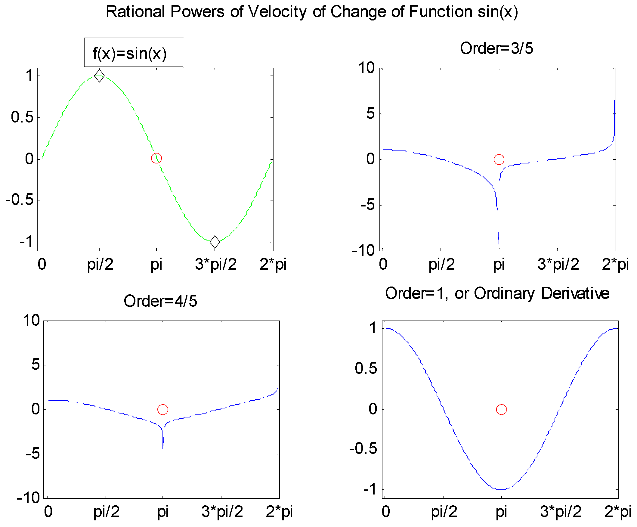
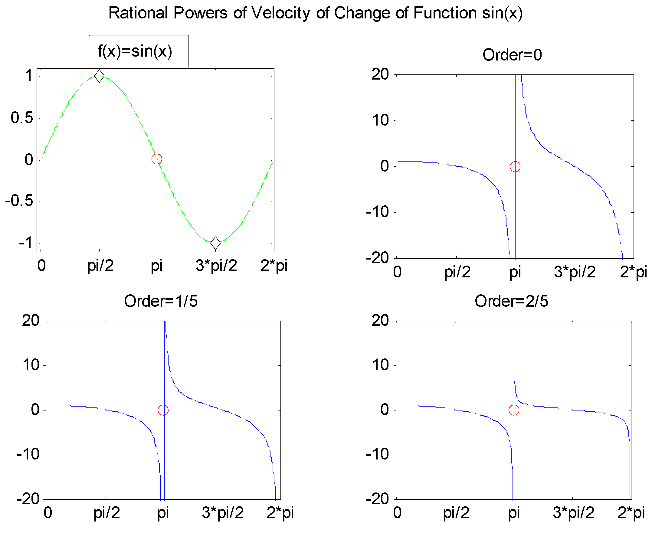
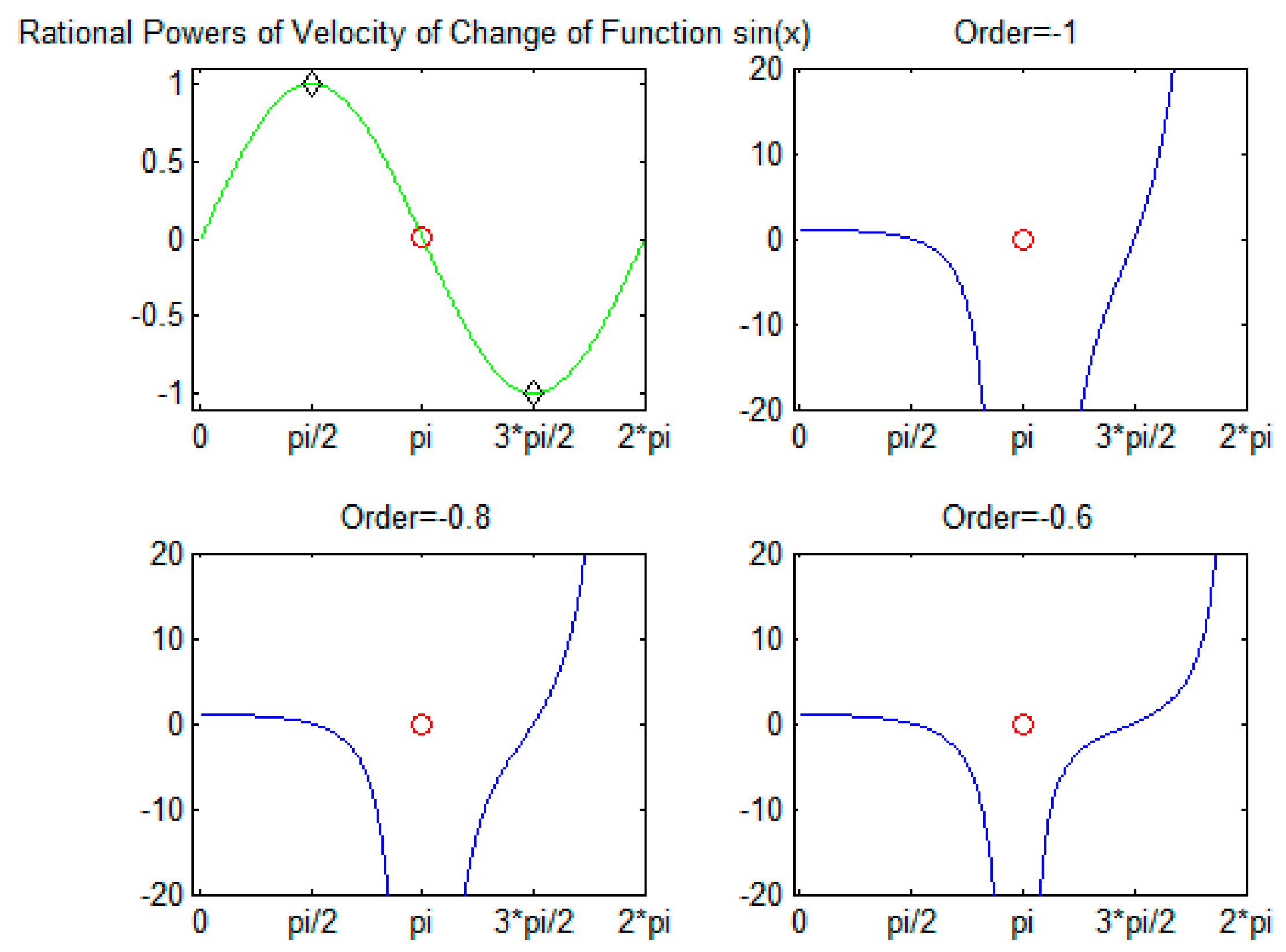
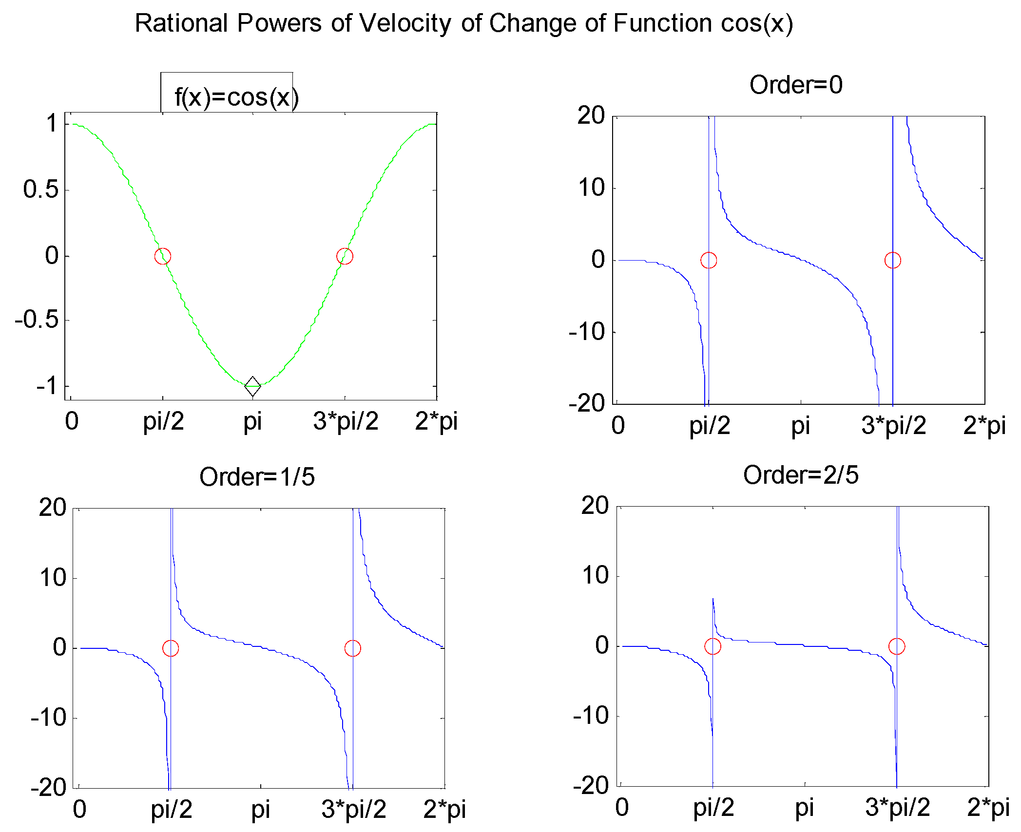
Figure 2 and Figure 3 show the rates of changes for sine functions and the obtained results support the claims of Figure 1. The red circles in both figures depict the inflection points. Figure 4 and Figure 5 depict the same cases for the cosine function. In the case of Figure 3 and Figure 5, while power is equal to 1, the rate of change is the same as an ordinary derivative. The domains of sine and cosine functions were determined as a period of functions. The inflection points for sine function are {(0, 0), (0, π), (0, 2π)} and large changes occur at these points for sine function (Figure 2 and Figure 3). The inflection points for cosine function are {(π/2, 0), (3π/2, 0} and large changes occur at these points for cosine function (Figure 4 and Figure 5).

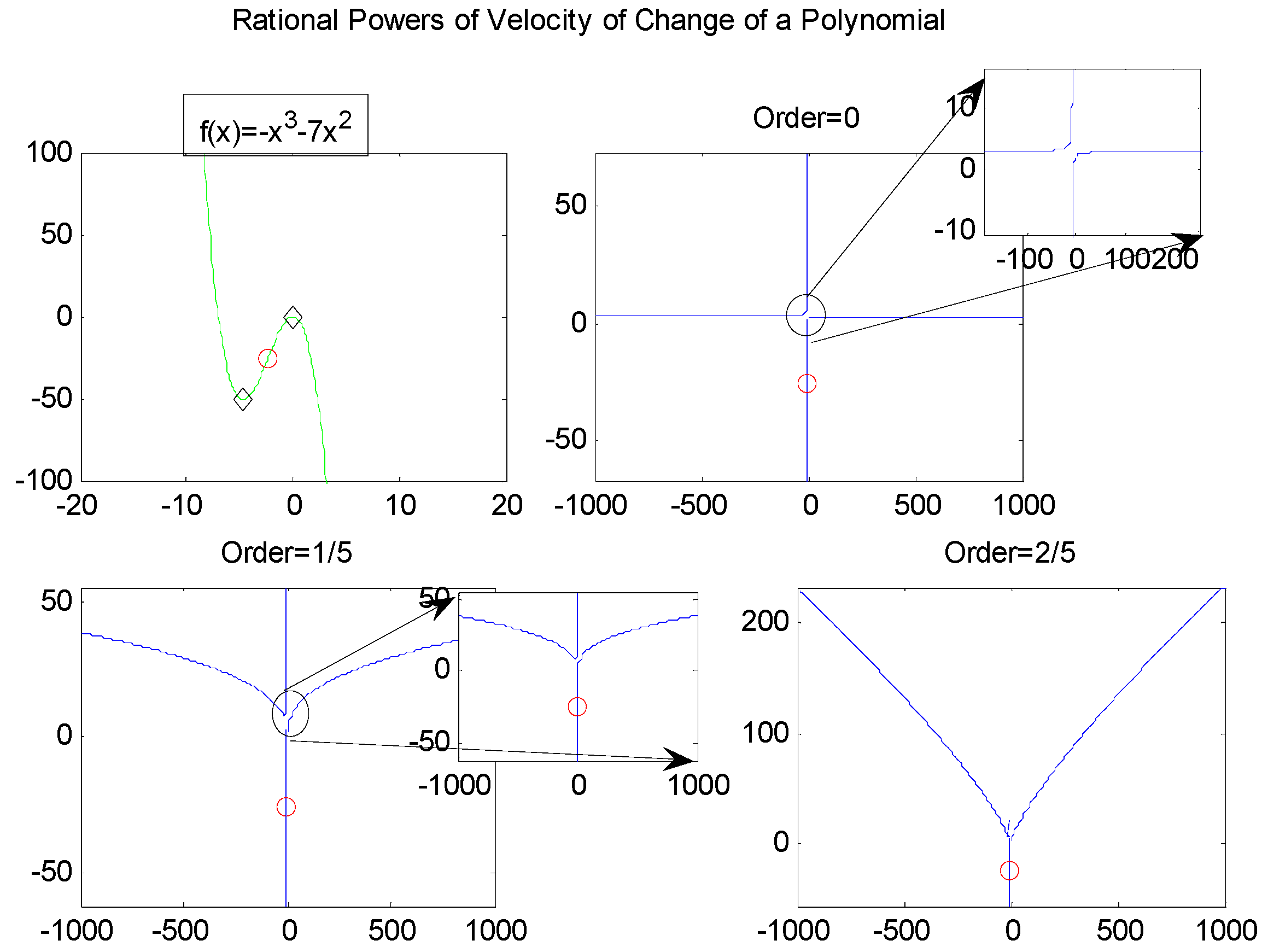
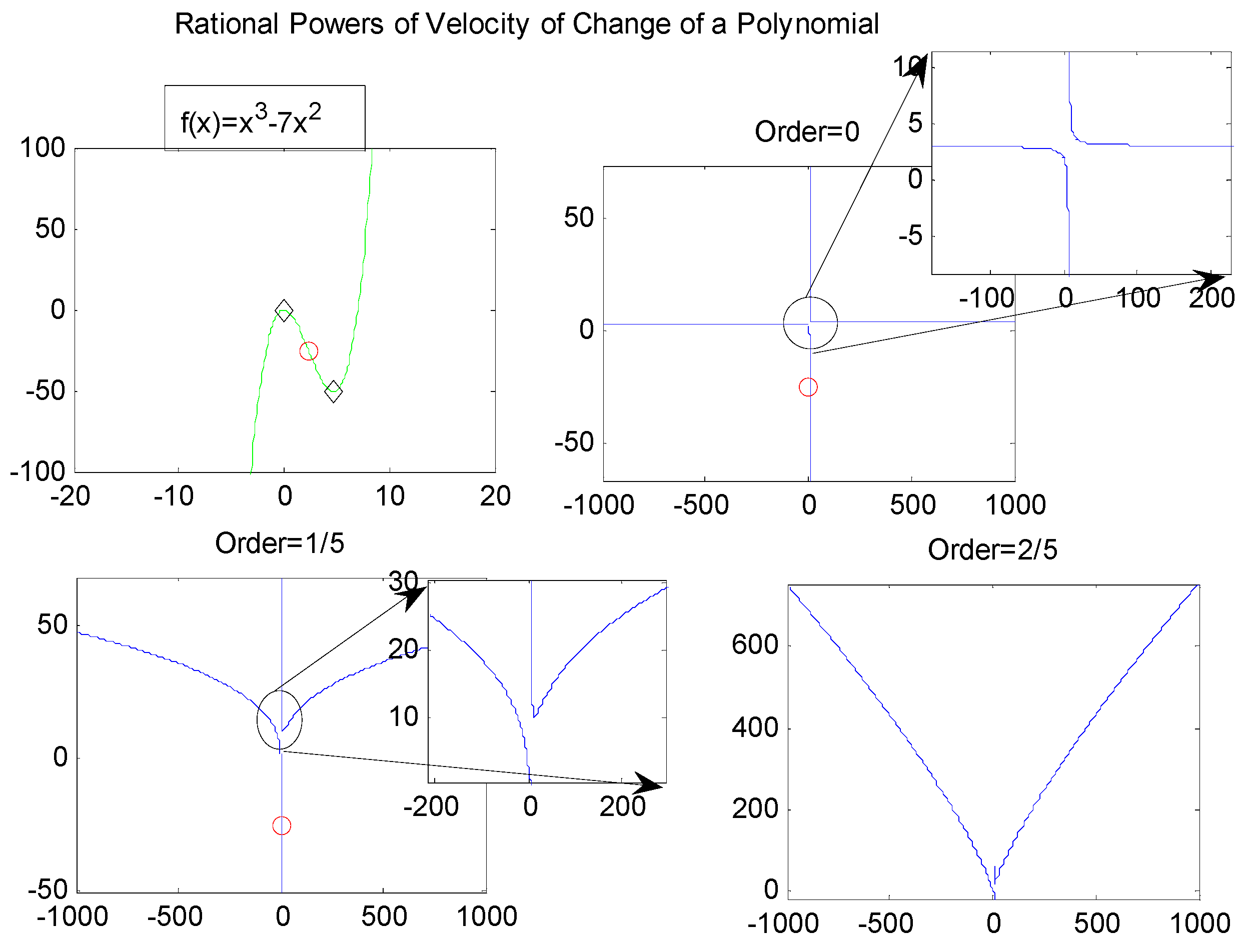
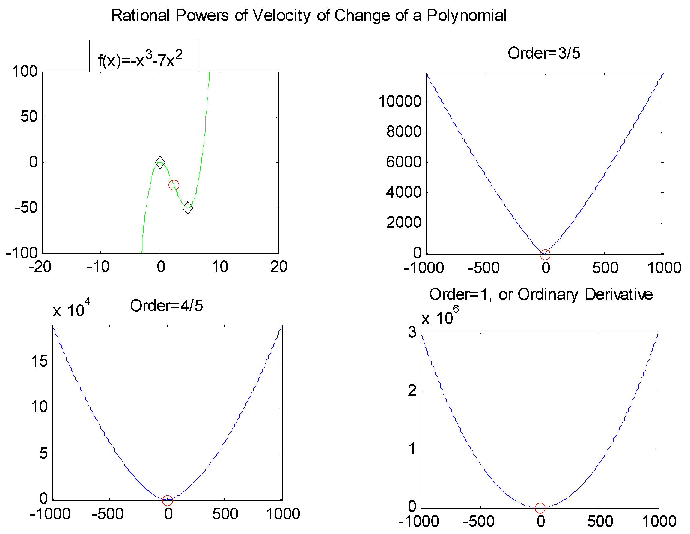
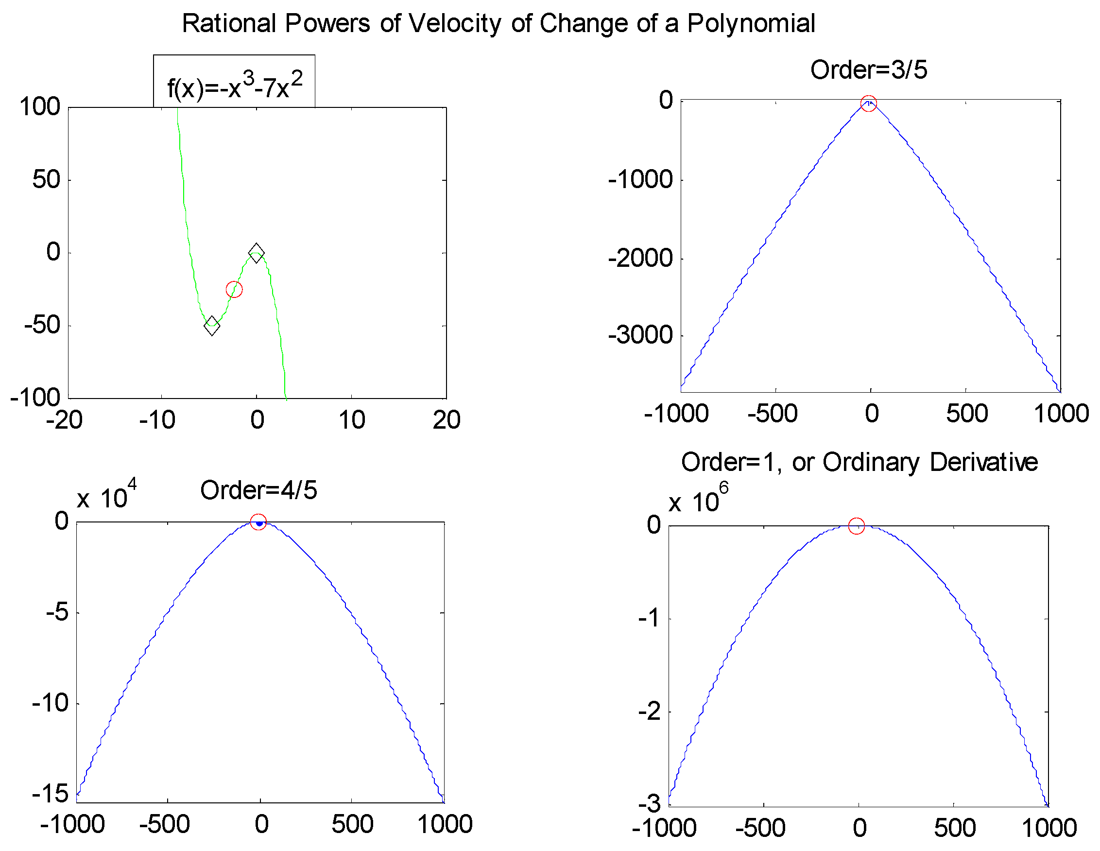
The same idea can be argued for polynomial functions, specifically functions f(x) = x³ − 7x² for $x\in [-1000,1000]$ and f(x) = −x³ − 7x² for $x\in [-1000,1000]$. The domains for these functions were selected to cover the inflection points and extremum points. The inflection point for f(x) = x³ − 7x² is (7/3, 1372/27); it is illustrated by a red circle. The inflection point for f(x) = −x³ − 7x² is (−7/3, −686/27); it is also illustrated by a red circle. The black diamond points are extremum points for both functions. The approach in Section 2 was verified by applications for polynomials as seen in Figure 6, Figure 7, Figure 8 and Figure 9.

A similar case can be considered for negative order, and to this end, sine function was selected for illustration. Figure 10 illustrates that in the case of negative orders, the same comments can be made for fractional order derivatives. The negative order reverses the direction of the increase/decrease, so the inequalities in Section 2 can be rephrased.

4. Analytical Approach and Results

The meaning of derivative is the rate of change or velocity of change in the dependent variable versus the changes in the independent variables [23,24,25]. Thus, the derivative of f(x) = cx⁰ is:

$$\begin{array}{c}\text{lim}\\ h\to 0\end{array}\frac{f(x+h)-f(x)}{(x+h)-x}=\begin{array}{c}\text{lim}\\ h\to 0\end{array}\frac{c-c}{h}=0$$

In the case of an identity function, it is:

$$\begin{array}{c}\text{lim}\\ h\to 0\end{array}\frac{f(x+h)-f(x)}{(x+h)-x}=\begin{array}{c}\text{lim}\\ h\to 0\end{array}\frac{(x+h)-x}{(x+h)-x}=1$$

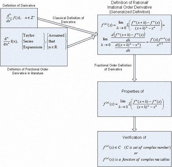
So, the definition for rational/irrational order derivative can be considered as follows.

Definition 1. 

f(x): R → R is a function, $\mathsf{\alpha }\in R$ and the rational/irrational order derivative can be considered as follows:

$$f^{(\mathsf{\alpha })}(x)=\begin{array}{c}\text{lim}\\ h\to 0\end{array}\frac{f^{\mathsf{\alpha }}(x+h)-f^{\mathsf{\alpha }}(x)}{{(x+h)}^{\mathsf{\alpha }}-x^{\mathsf{\alpha }}}$$

(1)

Before handling applications, the new definitions for rational/irrational order derivatives must be rephrased. Definition 1 is a classical definition of derivative, and it has an indefinite limit such that $\frac{0}{0}$, while h = 0. In this case, Definition 1 can be rephrased as seen in Definition 2.

Definition 2. 

Assume that f(x): R → R is a function, $\mathsf{\alpha }\in R$ and L(.) is a l’Hôpital process. The rational/irrational order derivative of f(x) is:

$$f^{(\mathsf{\alpha })}(x)=\begin{array}{c}\text{lim}\\ h\to 0\end{array}L\left(\frac{f^{\mathsf{\alpha }}(x+h)-f^{\mathsf{\alpha }}(x)}{{(x+h)}^{\mathsf{\alpha }}-x^{\mathsf{\alpha }}}\right)=\begin{array}{c}\text{lim}\\ h\to 0\end{array}\frac{\frac{d\left(f^{\mathsf{\alpha }}(x+h)-f^{\mathsf{\alpha }}(x)\right)}{dh}}{\frac{d({(x+h)}^{\mathsf{\alpha }}-x^{\mathsf{\alpha }})}{dh}}=\frac{f^{\prime }(x)f^{\mathsf{\alpha }-1}(x)}{x^{\mathsf{\alpha }-1}}$$

(2)

The new definition of rational/irrational order derivative (Definition 2) can be applied to some specific functions such as constant, identity, sine, and cosine functions. The velocity of change for a constant function is zero whatever the independent variable changes. The velocity of change for an identity function is 1 whatever the order of derivative and change of independent variable. The derivatives of sine, cosine, and polynomial functions for different orders are illustrated in Figure 2, Figure 3, Figure 4, Figure 5, Figure 6, Figure 7, Figure 8 and Figure 9.

These results demonstrated that the new definition obeys velocities of change of functions in extremum points, inflection points, etc.

The comments and descriptions in Section 2 can be supported with analytical results. The velocities of change of any functions can be expressed by derivatives. The point of this study is to analyze the powers of derivative with respect to all real powers.

Theorem 4.1. 

Assume that f(x) is any function such that f(x): R → R, and α₁, α₂, …, ${\mathsf{\alpha }}_n\in R^{+}$. Let f(x) be a positive, monotonically increasing/decreasing function in which the following conditions hold:

(a) 

If α₁, α₂, …, ${\mathsf{\alpha }}_n\in R^{+}$, α₁ ≤ α₂ ≤ … ≤ α_n and f(x) is positive and monotonically increasing, then $f^{({\mathsf{\alpha }}_1)}(x)\le f^{({\mathsf{\alpha }}_2)}(x)\le \mathrm{.....}\le f^{({\mathsf{\alpha }}_{n-1})}(x)\le f^{({\mathsf{\alpha }}_n)}(x)$.

(b) 

If α₁, α₂, …, ${\mathsf{\alpha }}_n\in R^{+}$, α₁ ≤ α₂ ≤ … ≤ α_n, and f(x) is positive and monotonically decreasing, then $f^{({\mathsf{\alpha }}_1)}(x)\ge f^{({\mathsf{\alpha }}_2)}(x)\ge \mathrm{.....}\ge f^{({\mathsf{\alpha }}_{n-1})}(x)\ge f^{({\mathsf{\alpha }}_n)}(x)$.

Proof. 

(a)

f(x) is a monotonically increasing function, so f(x_i) ≤ f(x_j) for x_i ≤ x_j, $\forall x_i,x_j\in R$. Then $f^{{\mathsf{\alpha }}_i}(x_k+h)\le f^{{\mathsf{\alpha }}_j}(x_k+h)$ and $f^{{\mathsf{\alpha }}_i}(x_k)\le f^{{\mathsf{\alpha }}_j}(x_k)$ where 1 ≤ i < j ≤ n, k is any index, α_i, α_j are two constants and α_i ≤ α_j. This case implies that $f^{({\mathsf{\alpha }}_i)}(x_k+h)-f^{({\mathsf{\alpha }}_i)}(x_k)\le f^{{\mathsf{\alpha }}_j}(x_k+h)-f^{({\mathsf{\alpha }}_j)}(x_k)$ and ${\left(x_k+h\right)}^{{\mathsf{\alpha }}_i}-x_k^{{\mathsf{\alpha }}_i}\le {\left(x_k+h\right)}^{{\mathsf{\alpha }}_j}-x_k^{{\mathsf{\alpha }}_j}$. So, this implies the following quotient:

$$\begin{array}{c}\text{lim}\\ h\to 0\end{array}L\left(\frac{f^{{\mathsf{\alpha }}_i}(x_k+h)-f^{{\mathsf{\alpha }}_i}(x_k)}{{(x_k+h)}^{{\mathsf{\alpha }}_i}-x_k^{{\mathsf{\alpha }}_i}}\right)\le \begin{array}{c}\text{lim}\\ h\to 0\end{array}L\left(\frac{f^{{\mathsf{\alpha }}_j}(x_k+h)-f^{{\mathsf{\alpha }}_j}(x_k)}{{(x_k+h)}^{{\mathsf{\alpha }}_j}-x_k^{{\mathsf{\alpha }}_j}}\right)$$

This implies the following important relations.

Step 1. 

Assuming that n = 2, there are two rational/irrational powers of functions such as α₁, ${\mathsf{\alpha }}_2\in R^{+}$, α₁ ≤ α₂. Then:

$$\begin{array}{c}\text{lim}\\ h\to 0\end{array}L\left(\frac{f^{{\mathsf{\alpha }}_1}(x_k+h)-f^{{\mathsf{\alpha }}_1}(x_k)}{{(x_k+h)}^{{\mathsf{\alpha }}_1}-x_k^{{\mathsf{\alpha }}_1}}\right)\le \begin{array}{c}\text{lim}\\ h\to 0\end{array}L\left(\frac{f^{{\mathsf{\alpha }}_2}(x_k+h)-f^{{\mathsf{\alpha }}_2}(x_k)}{{(x_k+h)}^{{\mathsf{\alpha }}_2}-x_k^{{\mathsf{\alpha }}_2}}\right)$$

Step 2. 

Assuming that there are n − 1 rational/irrational powers of rates of change, there are n − 1 rational/irrational powers of functions such as α₁, α₂, …, ${\mathsf{\alpha }}_{n-1}\in R^{+}$, α₁ ≤ α₂… ≤ α_n-1. Then:

$$\begin{array}{c}\text{lim}\\ h\to 0\end{array}L\left(\frac{f^{{\mathsf{\alpha }}_1}(x_k+h)-f^{{\mathsf{\alpha }}_1}(x_k)}{{(x_k+h)}^{{\mathsf{\alpha }}_1}-x_k^{{\mathsf{\alpha }}_1}}\right)\le \begin{array}{c}\text{lim}\\ h\to 0\end{array}L\left(\frac{f^{{\mathsf{\alpha }}_2}(x_k+h)-f^{{\mathsf{\alpha }}_2}(x_k)}{{(x_k+h)}^{{\mathsf{\alpha }}_2}-x_k^{{\mathsf{\alpha }}_2}}\right)\le \mathrm{...}\le \begin{array}{c}\text{lim}\\ h\to 0\end{array}L\left(\frac{f^{{\mathsf{\alpha }}_{n-1}}(x_k+h)-f^{{\mathsf{\alpha }}_{n-1}}(x_k)}{{(x_k+h)}^{{\mathsf{\alpha }}_{n-1}}-x_k^{{\mathsf{\alpha }}_{n-1}}}\right)$$

Step 3. 

Assuming that α₁, α₂, …, ${\mathsf{\alpha }}_n\in R^{+}$, α₁ ≤ α₂ ≤ … ≤ α_n, the following inequality holds:

$$f^{(n-1)}(x)=\begin{array}{c}\text{lim}\\ h\to 0\end{array}L\left(\frac{f^{{\mathsf{\alpha }}_{n-1}}(x_k+h)-f^{{\mathsf{\alpha }}_{n-1}}(x_k)}{{(x_k+h)}^{{\mathsf{\alpha }}_{n-1}}-x_k^{{\mathsf{\alpha }}_{n-1}}}\right)\le \begin{array}{c}\text{lim}\\ h\to 0\end{array}L\left(\frac{f^{{\mathsf{\alpha }}_n}(x_k+h)-f^{{\mathsf{\alpha }}_n}(x_k)}{{(x_k+h)}^{{\mathsf{\alpha }}_n}-x_k^{{\mathsf{\alpha }}_n}}\right)=f^{(n)}(x).$$

This means that $f^{({\mathsf{\alpha }}_{n-1})}(x)\le f^{({\mathsf{\alpha }}_n)}(x)$ and $f^{({\mathsf{\alpha }}_i)}(x)\le f^{({\mathsf{\alpha }}_n)}(x)$ for 1 ≤ i ≤ n − 1.

(b)

f(x) is a monotonically decreasing function, so f(x_i) ≥ f(x_j) for x_i ≤ x_j, $\forall x_i,x_j\in R$. Then $f^{{\mathsf{\alpha }}_i}(x_k+h)\ge f^{{\mathsf{\alpha }}_j}(x_k+h)$ and $f^{{\mathsf{\alpha }}_i}(x_k)\ge f^{{\mathsf{\alpha }}_j}(x_k)$ where 1 ≤ i < j ≤ n, k is any index, α_i, α_j are two constants and α_i ≤ α_j. This case implies that $f^{({\mathsf{\alpha }}_i)}(x_k+h)-f^{({\mathsf{\alpha }}_i)}(x_k)\ge f^{{\mathsf{\alpha }}_j}(x_k+h)-f^{({\mathsf{\alpha }}_j)}(x_k)$ and ${\left(x_k+h\right)}^{{\mathsf{\alpha }}_i}-x_k^{{\mathsf{\alpha }}_i}\le {\left(x_k+h\right)}^{{\mathsf{\alpha }}_j}-x_k^{{\mathsf{\alpha }}_j}$. So, this implies the following quotient:

$$\begin{array}{c}\text{lim}\\ h\to 0\end{array}L\left(\frac{f^{{\mathsf{\alpha }}_i}(x_k+h)-f^{{\mathsf{\alpha }}_i}(x_k)}{{(x_k+h)}^{{\mathsf{\alpha }}_i}-x_k^{{\mathsf{\alpha }}_i}}\right)\ge \begin{array}{c}\text{lim}\\ h\to 0\end{array}L\left(\frac{f^{{\mathsf{\alpha }}_j}(x_k+h)-f^{{\mathsf{\alpha }}_j}(x_k)}{{(x_k+h)}^{{\mathsf{\alpha }}_j}-x_k^{{\mathsf{\alpha }}_j}}\right)$$

This implies the following important relations.

Step 1. 

Assuming that n = 2, there are two rational/irrational powers of functions such as α₁, ${\mathsf{\alpha }}_2\in R^{+}$, α₁ ≤ α₂. Then:

$$\begin{array}{c}\text{lim}\\ h\to 0\end{array}L\left(\frac{f^{{\mathsf{\alpha }}_1}(x_k+h)-f^{{\mathsf{\alpha }}_1}(x_k)}{{(x_k+h)}^{{\mathsf{\alpha }}_1}-x_k^{{\mathsf{\alpha }}_1}}\right)\ge \begin{array}{c}\text{lim}\\ h\to 0\end{array}L\left(\frac{f^{{\mathsf{\alpha }}_2}(x_k+h)-f^{{\mathsf{\alpha }}_2}(x_k)}{{(x_k+h)}^{{\mathsf{\alpha }}_2}-x_k^{{\mathsf{\alpha }}_2}}\right)$$

Step 2. 

Assuming that there are n − 1 rational/irrational powers of rates of changes, then there are n − 1 rational/irrational powers of functions such as α₁, α₂, …, ${\mathsf{\alpha }}_{n-1}\in R^{+}$, α₁ ≤ α₂…. ≤ α_n-1. Then:

$$\begin{array}{c}\text{lim}\\ h\to 0\end{array}L\left(\frac{f^{{\mathsf{\alpha }}_1}(x_k+h)-f^{{\mathsf{\alpha }}_1}(x_k)}{{(x_k+h)}^{{\mathsf{\alpha }}_1}-x_k^{{\mathsf{\alpha }}_1}}\right)\le \begin{array}{c}\text{lim}\\ h\to 0\end{array}L\left(\frac{f^{{\mathsf{\alpha }}_2}(x_k+h)-f^{{\mathsf{\alpha }}_2}(x_k)}{{(x_k+h)}^{{\mathsf{\alpha }}_2}-x_k^{{\mathsf{\alpha }}_2}}\right)\le \mathrm{...}\le \begin{array}{c}\text{lim}\\ h\to 0\end{array}L\left(\frac{f^{{\mathsf{\alpha }}_{n-1}}(x_k+h)-f^{{\mathsf{\alpha }}_{n-1}}(x_k)}{{(x_k+h)}^{{\mathsf{\alpha }}_{n-1}}-x_k^{{\mathsf{\alpha }}_{n-1}}}\right)$$

Step 3. 

Assuming that α₁, α₂, …, ${\mathsf{\alpha }}_n\in R^{+}$, α₁ ≤ α₂ ≤ … ≤ α_n, the following inequality holds:

$$f^{(n-1)}(x)=\begin{array}{c}\text{lim}\\ h\to 0\end{array}L\left(\frac{f^{{\mathsf{\alpha }}_{n-1}}(x_k+h)-f^{{\mathsf{\alpha }}_{n-1}}(x_k)}{{(x_k+h)}^{{\mathsf{\alpha }}_{n-1}}-x_k^{{\mathsf{\alpha }}_{n-1}}}\right)\le \begin{array}{c}\text{lim}\\ h\to 0\end{array}L\left(\frac{f^{{\mathsf{\alpha }}_n}(x_k+h)-f^{{\mathsf{\alpha }}_n}(x_k)}{{(x_k+h)}^{{\mathsf{\alpha }}_n}-x_k^{{\mathsf{\alpha }}_n}}\right)=f^{(n)}(x)$$

This means that $f^{({\mathsf{\alpha }}_{n-1})}(x)\le f^{({\mathsf{\alpha }}_n)}(x)$ and $f^{({\mathsf{\alpha }}_i)}(x)\le f^{({\mathsf{\alpha }}_n)}(x)$for 1 ≤ i ≤ n − 1.

Theorem 4.2. 

Assume that f(x) is any function such that f(x): R → R, and α₁, α₂, …, ${\mathsf{\alpha }}_n\in R^{-}$. Let f(x) be a positive, monotonically increasing/decreasing function in which the following conditions hold:

(a) 

If α₁, α₂, …, ${\mathsf{\alpha }}_n\in R^{-}$, α₁ ≥ α₂ ≥ … ≥ α_n and f(x) is positive and monotonically increasing, then $f^{({\mathsf{\alpha }}_1)}(x)\ge f^{({\mathsf{\alpha }}_2)}(x)\ge \mathrm{...}\ge f^{({\mathsf{\alpha }}_{n-1})}(x)\ge f^{({\mathsf{\alpha }}_n)}(x)$.

(b) 

If α₁, α₂, …, ${\mathsf{\alpha }}_n\in R^{-}$, α₁ ≥ α₂ ≥ … ≥ α_n, and f(x) is positive and monotonically decreasing, then $f^{({\mathsf{\alpha }}_1)}(x)\ge f^{({\mathsf{\alpha }}_2)}(x)\ge \mathrm{.....}\ge f^{({\mathsf{\alpha }}_{n-1})}(x)\ge f^{({\mathsf{\alpha }}_n)}(x)$.

Proof. 

The proof can be handled in two steps: increasing function and decreasing function.

(a)

f(x) is a positive, monotonically increasing function, so f(x_i) ≤ f(x_j) for x_i ≤ x_j, $\forall x_i,x_j\in R$, and α₁, ${\mathsf{\alpha }}_2\in R^{-}$ and α₁ ≤ α₂. Then $f^{{\mathsf{\alpha }}_1}(x+h)\ge f^{{\mathsf{\alpha }}_2}(x+h)$ and $f^{{\mathsf{\alpha }}_1}(x)\ge f^{{\mathsf{\alpha }}_2}(x)$, |α₁| ≥ |α₂|.

$$A=\begin{array}{c}\text{lim}\\ h\to 0\end{array}L\left(\frac{f^{{\mathsf{\alpha }}_1}(x_i+h)-f^{{\mathsf{\alpha }}_1}(x_i)}{{(x_i+h)}^{{\mathsf{\alpha }}_1}-x_i^{{\mathsf{\alpha }}_1}}\right)=\frac{\frac{d}{dh}\frac{\left(f^{\left|{\mathsf{\alpha }}_1\right|}(x)-f^{\left|{\mathsf{\alpha }}_1\right|}(x+h)\right)}{f^{\left|{\mathsf{\alpha }}_1\right|}(x)f^{\left|{\mathsf{\alpha }}_1\right|}(x+h)}}{\frac{d}{dh}\frac{x^{\left|{\mathsf{\alpha }}_1\right|}-{(x+h)}^{\left|{\mathsf{\alpha }}_1\right|}}{x^{\left|{\mathsf{\alpha }}_1\right|}{(x+h)}^{\left|{\mathsf{\alpha }}_1\right|}}}=\frac{f^{\prime }(x){\left(x\right)}^{\left|{\mathsf{\alpha }}_1\right|+1}}{f^{\left|{\mathsf{\alpha }}_1\right|+1}(x)}$$

and,

$$B=\begin{array}{c}\text{lim}\\ h\to 0\end{array}L\left(\frac{f^{{\mathsf{\alpha }}_2}(x_i+h)-f^{{\mathsf{\alpha }}_2}(x_i)}{{(x_i+h)}^{{\mathsf{\alpha }}_2}-x_i^{{\mathsf{\alpha }}_2}}\right)=\frac{\frac{d}{dh}\frac{\left(f^{\left|{\mathsf{\alpha }}_2\right|}(x)-f^{\left|{\mathsf{\alpha }}_2\right|}(x+h)\right)}{f^{\left|{\mathsf{\alpha }}_2\right|}(x)f^{\left|{\mathsf{\alpha }}_2\right|}(x+h)}}{\frac{d}{dh}\frac{x^{\left|{\mathsf{\alpha }}_2\right|}-{(x+h)}^{\left|{\mathsf{\alpha }}_2\right|}}{x^{\left|{\mathsf{\alpha }}_2\right|}{(x+h)}^{\left|{\mathsf{\alpha }}_2\right|}}}=\frac{f^{\prime }(x){\left(x\right)}^{\left|{\mathsf{\alpha }}_2\right|+1}}{f^{\left|{\mathsf{\alpha }}_2\right|+1}(x)}$$

where $f^{\left|{\mathsf{\alpha }}_1\right|+1}(x)\le f^{\left|{\mathsf{\alpha }}_2\right|+1}(x)$ and $x^{\left|{\mathsf{\alpha }}_1\right|+1}\le x^{\left|{\mathsf{\alpha }}_2\right|+1}$. This case implies the following inequality:

$$A\ge B\Rightarrow \frac{f^{\prime }(x){\left(x\right)}^{\left|{\mathsf{\alpha }}_1\right|+1}}{f^{\left|{\mathsf{\alpha }}_1\right|+1}(x)}\ge \frac{f^{\prime }(x){\left(x\right)}^{\left|{\mathsf{\alpha }}_2\right|+1}}{f^{\left|{\mathsf{\alpha }}_2\right|+1}(x)}\Rightarrow \frac{{\left(x\right)}^{\left|{\mathsf{\alpha }}_1\right|+1}}{f^{\left|{\mathsf{\alpha }}_1\right|+1}(x)}\ge \frac{{\left(x\right)}^{\left|{\mathsf{\alpha }}_2\right|+1}}{f^{\left|{\mathsf{\alpha }}_2\right|+1}(x)}$$

This case is for two orders, and it can be enlarged to other orders. For α₁ ≥ α₂ ≥ … ≥ α_n and |α₁| ≤ |α₂| ≤ … ≤ |α_n|,

$$\frac{f^{\prime }(x){\left(x\right)}^{\left|{\mathsf{\alpha }}_1\right|+1}}{f^{\left|{\mathsf{\alpha }}_1\right|+1}(x)}\ge \frac{f^{\prime }(x){\left(x\right)}^{\left|{\mathsf{\alpha }}_2\right|+1}}{f^{\left|{\mathsf{\alpha }}_2\right|+1}(x)}\ge \mathrm{...}\ge \frac{{\left(x\right)}^{\left|{\mathsf{\alpha }}_{n-1}\right|+1}}{f^{\left|{\mathsf{\alpha }}_{n-1}\right|+1}(x)}\ge \frac{{\left(x\right)}^{\left|{\mathsf{\alpha }}_n\right|+1}}{f^{\left|{\mathsf{\alpha }}_n\right|+1}(x)}$$

(b)

g(x) is a positive, monotonically decreasing function, so g(x_i) ≥ g(x_j) for x_i ≤ x_j, $\forall x_i,x_j\in R$, and α₁, ${\mathsf{\alpha }}_2\in R^{-}$ and α₁ ≤ α₂. Then $g^{{\mathsf{\alpha }}_1}(x+h)\le g^{{\mathsf{\alpha }}_2}(x+h)$ and $g^{{\mathsf{\alpha }}_1}(x)\le g^{{\mathsf{\alpha }}_2}(x)$, |α₁| ≥ |α₂|. Assuming that f(x) is a positive, monotonically increasing function, $g(x)=\frac{1}{f(x)}$ is a positive, monotonically decreasing function:

$$A=\begin{array}{c}\text{lim}\\ h\to 0\end{array}L\left(\frac{g^{{\mathsf{\alpha }}_1}(x_i+h)-g^{{\mathsf{\alpha }}_1}(x_i)}{{(x_i+h)}^{{\mathsf{\alpha }}_1}-x_i^{{\mathsf{\alpha }}_1}}\right)=\frac{\frac{d}{dh}\left(f^{\left|{\mathsf{\alpha }}_1\right|}(x+h)-f^{\left|{\mathsf{\alpha }}_1\right|}(x)\right)}{\frac{d}{dh}\frac{x^{\left|{\mathsf{\alpha }}_1\right|}-{(x+h)}^{\left|{\mathsf{\alpha }}_1\right|}}{x^{\left|{\mathsf{\alpha }}_1\right|}{(x+h)}^{\left|{\mathsf{\alpha }}_1\right|}}}=-\frac{f^{\prime }(x)f^{\left|{\mathsf{\alpha }}_1\right|-1}(x)}{x^{3\left|{\mathsf{\alpha }}_1\right|-1}}$$

and,

$$B=\begin{array}{c}\text{lim}\\ h\to 0\end{array}L\left(\frac{g^{{\mathsf{\alpha }}_2}(x_i+h)-g^{{\mathsf{\alpha }}_2}(x_i)}{{(x_i+h)}^{{\mathsf{\alpha }}_2}-x_i^{{\mathsf{\alpha }}_2}}\right)=\frac{\frac{d}{dh}\left(f^{\left|{\mathsf{\alpha }}_2\right|}(x+h)-f^{\left|{\mathsf{\alpha }}_2\right|}(x)\right)}{\frac{d}{dh}\frac{x^{\left|{\mathsf{\alpha }}_2\right|}-{(x+h)}^{\left|{\mathsf{\alpha }}_2\right|}}{x^{\left|{\mathsf{\alpha }}_2\right|}{(x+h)}^{\left|{\mathsf{\alpha }}_2\right|}}}=-\frac{f^{\prime }(x)f^{\left|{\mathsf{\alpha }}_2\right|-1}(x)}{x^{3\left|{\mathsf{\alpha }}_2\right|-1}}$$

where $f^{\left|{\mathsf{\alpha }}_2\right|-1}(x)\le f^{\left|{\mathsf{\alpha }}_1\right|-1}(x)$ and $x^{3\left|{\mathsf{\alpha }}_2\right|-1}\le x^{3\left|{\mathsf{\alpha }}_1\right|-1}$. This case implies the following inequality.

$$A\le B\Rightarrow -\frac{f^{\prime }(x)f^{\left|{\mathsf{\alpha }}_1\right|-1}(x)}{x^{3\left|{\mathsf{\alpha }}_1\right|-1}}\ge -\frac{f^{\prime }(x)f^{\left|{\mathsf{\alpha }}_2\right|-1}(x)}{x^{3\left|{\mathsf{\alpha }}_2\right|-1}}\Rightarrow -\frac{f^{\prime }(x)f^{\left|{\mathsf{\alpha }}_1\right|-1}(x)}{x^{3\left|{\mathsf{\alpha }}_1\right|-1}}\ge -\frac{f^{\prime }(x)f^{\left|{\mathsf{\alpha }}_2\right|-1}(x)}{x^{3\left|{\mathsf{\alpha }}_2\right|-1}}$$

This case is for two orders, and it can be enlarged to other orders. For α₁ ≥ α₂ ≥ … ≥ α_n and |α₁| ≤ |α₂| ≤ … ≤ |α_n|,

$$-\frac{f^{\prime }(x){\left(x\right)}^{\left|{\mathsf{\alpha }}_1\right|-1}}{f^{\left|{\mathsf{\alpha }}_1\right|-1}(x)}\ge \frac{f^{\prime }(x){\left(x\right)}^{\left|{\mathsf{\alpha }}_2\right|-1}}{f^{\left|{\mathsf{\alpha }}_2\right|-1}(x)}\ge \mathrm{...}\ge \frac{{\left(x\right)}^{\left|{\mathsf{\alpha }}_{n-1}\right|-1}}{f^{\left|{\mathsf{\alpha }}_{n-1}\right|-1}(x)}\ge \frac{{\left(x\right)}^{\left|{\mathsf{\alpha }}_n\right|-1}}{f^{\left|{\mathsf{\alpha }}_n\right|-1}(x)}$$

Any complex number has direction and magnitude. It is known that derivative has direction and magnitude. So the relationship between complex numbers and derivatives must be verified.

Theorem 4.3. 

Assuming that f(x) is a function such as f: R → R and $\mathsf{\alpha }\in R$, f^(α)(x) is a function of complex variables.

Proof. 

Assume that $\mathsf{\alpha }=\frac{\mathsf{\beta }}{\mathsf{\delta }}$ and δ ≠ 0. If f(x) ≥ 0, the obtained results are positive, and they constitute the real part of complex numbers. The rational/irrational order derivative of f(x) is:

$$f^{(\mathsf{\alpha })}=\frac{f^{\prime }(x)f^{\mathsf{\alpha }-1}(x)}{x^{\mathsf{\alpha }-1}}=f^{\prime }(x)\sqrt[\mathsf{\delta }]{\frac{f^{\mathsf{\beta }-\mathsf{\delta }}(x)}{x^{\mathsf{\beta }-\mathsf{\delta }}}}=f^{\prime }(x)\sqrt[\mathsf{\delta }]{{\left(\frac{f(x)}{x}\right)}^{\mathsf{\beta }-\mathsf{\delta }}}$$

If the rational/irrational derivative is a function of complex variables, then f^(α)(x) = g(x) + ih(x), where $i=\sqrt{-1}$.

If f(x) < 0, there will be two cases:

Case 1: 

Assume that δ is odd.

If ${\left(\frac{f(x)}{x}\right)}^{\mathsf{\beta }-\mathsf{\delta }}\ge 0$ or ${\left(\frac{f(x)}{x}\right)}^{\mathsf{\beta }-\mathsf{\delta }}<0$, then the obtained function f^(α)(x) is a real function and h(x) = 0 for both cases since the multiplication of any negative number in odd steps yields a negative number.

Case 2: 

Assume that δ is even.

If ${\left(\frac{f(x)}{x}\right)}^{\mathsf{\beta }-\mathsf{\delta }}\ge 0$, then h(x) = 0 and f^(α)(x) is a real function.

If ${\left(\frac{f(x)}{x}\right)}^{\mathsf{\beta }-\mathsf{\delta }}<0$, then the multiplication of any number in even steps yields a positive number for real numbers. However, it yields a negative result for complex numbers, so, h(x) ≠ 0. This means that f^(α)(x) is a complex function.

In fact, f^(α)(x) is a complex function for both cases because h(x) = 0 for some situations.

Problem 1. 

The derivative operator D is a linear operator. The theoretical and application results presented in the previous sections demonstrated that the derivative operator does not have to be linear. The ordinary derivative operator D is linear; however, the rate of change of any function versus its independent variables does not have to be linear. This is in need of theoretical verification.

Problem 2. 

A new approach for derivatives was expressed in this paper. This new approach has the potential to change the integration rules in the case of orders of derivatives different from 1. The new rules for integration should be defined.

Problem 3. 

The geometrical meanings of ordinary derivatives are known. The geometrical meanings of this new approach for derivatives in the case of rational and irrational orders of derivatives are still unknown.

5. Conclusions

The ordinary definition of a derivative from Newton and l’Hôpital can be considered as order = 1; in this case, the derivative operator D is linear. This paper includes a new approach for the derivative concept in which the derivative operator is not linear. The following consequences can be put forth:

(a)

All functions have maximum rates of changes at inflection points in the positive direction.

(b)

All functions have minimum rates of changes at inflection points in the negative direction.

(c)

The derivative operator does not have to be linear, since the rates of changes of functions are not linear.

(d)

This new approach needs to prove geometrical meaning for derivative orders different from 1.

(e)

This new approach brought out a new problem: how to handle the integration in cases of derivative orders different from 1.

(f)

This new approach reveals that derivative and complex numbers have relationships.