Data-Driven Computation Scheme for Duncan–Chang EB Model

Abstract

This paper extends the data-driven computational mechanics paradigm to nonlinear materials characterized by the Duncan–Chang Elastic-Bulk (E-B) constitutive model. Unlike in linear elastic systems, geotechnical media exhibit stress-dependent tangent moduli and non-convex constitutive manifolds. We propose a recursive nested data-driven solver that dynamically adapts the phase-space distance metric to account for pressure-dependent hardening. A rigorous mathematical analysis of convergence is provided, demonstrating that the solver’s performance is governed by the local transversality between the conservation law constraint set and the nonlinear material manifold. We derive explicit error bounds that couple spatial discretization resolution with material data density. Numerical experiments using triaxial test data from a high-altitude region validate the theoretical predictions, showing that the proposed scheme demonstrates convergence in single-element tests.

1. Introduction

1.1. The Duncan–Chang EB Model: Development and Limitations

The Duncan–Chang EB model represents one of the most widely adopted constitutive frameworks in computational geomechanics. Developed from extensive experimental observations of soil behavior under triaxial loading conditions, the model captures the essential features of granular material response including stress-dependent stiffness, nonlinear stress–strain relationships, and bulk modulus evolution [1]. The model characterizes soil behavior through a hyperbolic relationship between deviatoric stress and axial strain, with stress-dependent tangent moduli that capture the pressure-sensitive nature of granular materials. By virtue of its mathematical formulation, this model has been extensively applied in the analysis of earth dams, foundations, and slopes [2,3].

Since its inception, researchers have proposed numerous modifications and enhancements to the basic model. For example, Wang et al. [2] introduced dilatancy into the traditional Duncan–Chang EB model to develop an EBD constitutive model for rockfill materials, validated against monitoring data from the Aertashi concrete face rockfill dam. Dong et al. [4] modified the model based on triaxial consolidated drained test data for medium–coarse sand with different relative densities, enabling consideration of disturbance effects on soil response—particularly important for stability analysis of sand excavation.

Although the Duncan–Chang model has certain limitations and researchers have continuously proposed modifications to improve it [5,6], it is still extensively used in practice. Furthermore, the numerical implementation of the Duncan–Chang model has been explored using various finite element platforms. Sun et al. [7] and Qing-ming [8] developed implementations based on secondary development interfaces of commercial software, respectively, showing good agreement with experimental results. Nevertheless, the fundamental challenge of parameter calibration remains, motivating interest in alternative approaches.

Despite its empirical success, the Duncan–Chang model requires careful parameter calibration using curve-fitting procedures applied to experimental data—a process that introduces modeling error, parameter uncertainty, and potential loss of information. Traditional calibration methods often rely on selecting specific points from stress–strain curves (e.g., 75% and 90% of failure stress) or regression techniques [9], which may not always yield reasonable parameter values. In some cases, the modulus exponent parameter n can even become negative [1], raising questions about the physical meaning of the fitted parameters.

1.2. Data-Driven Computational Mechanics: A New Paradigm

Data-driven computational mechanics (DDCM) represents a paradigm shift from model-based to data-based approaches in solid mechanics [10]. Three main branches have emerged.

1.2.1. Model-Free Data-Driven Methods

Model-free methods directly incorporate stress–strain data into analysis, completely bypassing material model definition. Stöcker et al. [11] provides a comprehensive comparison of model-free and model-based approaches in constitutive modeling. The foundational work by González et al. [12] established the mathematical framework for consistent data-driven computational mechanics.

Key challenges in model-free DDCM include efficient data structures for nearest-neighbor searches in high-dimensional phase spaces. Eggersmann et al. [13] developed efficient data structures specifically for model-free data-driven computational mechanics, addressing computational bottlenecks. Gebhardt et al. [14] proposed a framework based on nonlinear optimization for data-driven structural analysis in general elasticity.

Wattel et al. [15] introduced mesh d-refinement as a novel data-based computational framework to account for complex material response through abstract phase spaces, avoiding explicit constitutive law definitions. This approach matches physically admissible states with observed material response data.

1.2.2. History-Dependent Behavior

The extension of DDCM to path-dependent and inelastic materials has been an active area of research. Dandin et al. [16] extended the data-driven framework to history-dependent behavior by representing the material response as a directed graph, where vertices represent strain–stress pairs and arcs represent thermodynamically admissible transitions. To account for complex inelastic phenomena such as plasticity and phase transformations, Bartel et al. [17] introduced the concept of history surrogates and propagators, enabling the enrichment of the material database with path-dependent information without altering the core distance-minimization structure. Karapiperis et al. [18] developed a multiscale data-driven framework where the material history of granular media, such as sand, is parameterized through lower-scale computations, effectively capturing non-monotonic loading responses and shear banding.

Beyond deterministic models, the quantification of uncertainty is a crucial frontier. Huang et al. [19] developed a sequential linear programming (SLP) approach for uncertainty analysis in data-driven computational mechanics, providing bound-based structural responses. Zschocke et al. [20] proposed a scheme for handling polymorphic uncertainties in composite materials by incorporating both aleatoric and epistemic uncertainties within a single dataset, thereby allowing for efficient macroscopic structural analysis in the presence of mesoscale heterogeneities.

1.2.3. Neural Network-Based Methods

Alternative data-driven approaches utilize artificial neural networks to approximate constitutive relationships. Zlatić et al. [10] compared neural network-based and model-free approaches for computational mechanics, finding that neural networks can learn material behavior patterns from data effectively. Ciftci and Hackl [21] proposed a physics-informed GAN framework based on model-free data-driven computational mechanics.

To clearly position our proposed framework within the broader landscape of data-driven mechanics, we provide a comparative analysis of the three main branches discussed above.

Table 1. Comparison of different data-driven computational mechanics (DDCM) approaches.

Feature	Model-Free DDCM (Distance Minimization)	Neural Network-Based Constitutive Modeling	Proposed Adaptive Metric DDCM (This Work)
Core Mechanism	Direct phase-space projection onto discrete dataset	Approximation of constitutive manifold via continuous functions	Phase-space projection with stress-dependent Riemannian metric
Data Fidelity	Exact adherence to data (zero modeling error at data points)	Smoothing/Fitting error exists	Exact adherence to data with physics-informed search direction
Stress Dependency	Difficult to handle without adaptive metric	Learned implicitly by NN architecture	Explicitly handled via nested stiffness update
Computational Cost	High (Nearest Neighbor Search)	Low (during inference)	Moderate to High (Iterative Metric Update + Search)
Interpretability	High (returns actual experimental points)	Low (Black-box)	High (returns actual experimental points)

highlights the key differences in terms of data requirements, computational efficiency, and applicability to stress-dependent materials.

1.3. Gap in Existing Studies and Current Contributions

The data-driven computing paradigm offers a fundamentally different approach: calculations proceed directly from experimental material data while satisfying conservation laws and kinematic constraints, thereby eliminating the intermediate modeling step [11]. This paradigm, pioneered by Kirchdoerfer and Ortiz [22], represents a transition from standard data-scarce methods to modern data-rich approaches in computational mechanics [10]. While previous work has demonstrated the viability of data-driven methods for linear elasticity [14] and simple nonlinear structures [12], extending this framework to stress-dependent hyperbolic materials presents several theoretical and computational challenges:

• High-dimensional phase space: The Duncan–Chang model operates in a 12-dimensional local phase space (six independent stress components and six independent strain components), with material response depending nonlinearly on the stress state itself.
• Pressure-dependent stiffness: Unlike classical elasticity, the tangent moduli in the Duncan–Chang model vary with confining pressure, requiring datasets that adequately sample this additional dimension.
• Hyperbolic stress–strain behavior: The asymptotic nature of hyperbolic relationships necessitates careful treatment of the failure envelope and appropriate penalty function formulation.
• Convergence analysis: Establishing convergence requires accounting for the non-polynomial nonlinearity of the constitutive manifold and its transversality properties with respect to equilibrium constraints.

In this work, we develop a comprehensive theoretical framework for data-driven computing with Duncan–Chang materials, including the following:

• Formulation of the data-driven problem for stress-dependent hyperbolic materials with appropriate distance metrics.
• Efficient algorithms for local data assignment in high-dimensional phase spaces.
• Rigorous convergence analysis with explicit error bounds.
• Extension to finite element discretizations with joint convergence in mesh size and data resolution.
• Numerical validation using real triaxial test data.

The remainder of this paper is organized as follows. Section 2 presents the classical Duncan–Chang EB model formulation and its phase space characterization. Section 3 develops the data-driven formulation for stress-dependent materials. Section 4 describes the iterative solution algorithm. Section 5 demonstrates the numerical applications and validation using triaxial test data. Section 6 presents the mathematical convergence analysis. Finally, Section 7 discusses the implications, limitations, and future directions of this work.

2. The Duncan–Chang EB Model

2.1. Classical Formulation

The Duncan–Chang EB model characterizes soil behavior through two primary relationships: a hyperbolic stress–strain curve for deviatoric behavior and a separate bulk modulus formulation for volumetric response.

2.1.1. Deviatoric Behavior

Under triaxial compression with axial strain ${\epsilon }_1$ and confining pressure ${\sigma }_3$, the deviatoric stress is given by

$${\sigma }_1-{\sigma }_3={\displaystyle \frac{{\epsilon }_1}{a+b{\epsilon }_1}}$$

(1)

where the parameters are defined as

$$a={\displaystyle \frac{1}{E_i}},b={\displaystyle \frac{1}{{({\sigma }_1-{\sigma }_3)}_f}}$$

(2)

The initial tangent modulus is

$$E_i=K{P}_a{\left({\displaystyle \frac{{\sigma }_3}{P_a}}\right)}^n$$

(3)

where K is the modulus number, n is the modulus exponent, and $P_a$ is the atmospheric pressure (reference stress). The failure stress difference is

$${({\sigma }_1-{\sigma }_3)}_f={\displaystyle \frac{2ccos\varphi +2{\sigma }_{3}sin\varphi }{1-sin\varphi }}·R_f$$

(4)

where c is cohesion, $\varphi$ is the friction angle, and $R_f$ is the failure ratio (typically 0.75–0.95).

2.1.2. Tangent Modulus

The stress-dependent tangent Young’s modulus is given by

$$E_t=K{P}_a{\left({\displaystyle \frac{{\sigma }_3}{P_a}}\right)}^n{\left[1-{\displaystyle \frac{R_f(1-sin\varphi )({\sigma }_1-{\sigma }_3)}{2ccos\varphi +2{\sigma }_{3}sin\varphi }}\right]}^2$$

(5)

where $R_f$ is the failure ratio. This formulation captures the degradation of stiffness as the stress state approaches the failure envelope.

2.1.3. Bulk Modulus

The volumetric response is characterized by

$$B=K_b{P}_a{\left({\displaystyle \frac{{\sigma }_3}{P_a}}\right)}^m$$

(6)

where $K_b$ is the bulk modulus number and m is the bulk modulus exponent.

2.2. Material Datasets

A material dataset for the Duncan–Chang model consists of stress–strain pairs obtained from laboratory testing:

$$\mathcal{E}=\{({\mathit{\epsilon }}^{\left(i\right)},{\mathit{\sigma }}^{\left(i\right)}):i=1,\dots ,N\}$$

(7)

Ideally, these points are obtained from multiple triaxial tests at different confining pressures, consolidated undrained (CU) tests, or isotropic compression tests to capture the full pressure-dependent behavior. Each data point represents a material state that is physically realizable and experimentally verified.

Unlike linear elastic materials where a single test can theoretically determine all material parameters, Duncan–Chang materials require systematic sampling across the relevant stress space to capture pressure-dependent stiffness variations.

2.3. Phase Space and Constitutive Manifold

For three-dimensional problems, the local state is characterized by the pair $z=(\mathit{ϵ},\mathit{\sigma })\in \mathcal{Z}$. We introduce a stress-dependent reference stiffness ${\mathbb{C}}_{ref}$ (equivalent to the initial stiffness $E_i$ in Equation (2)) to define a local metric in the phase space:

$${\left|z\right|}_{{\mathbb{C}}_{ref}}^2={\displaystyle \frac{1}{2}}\mathit{ϵ}:{\mathbb{C}}_{ref}:\mathit{ϵ}+{\displaystyle \frac{1}{2}}\mathit{\sigma }:{\mathbb{C}}_{ref}^{-1}:\mathit{\sigma }$$

(8)

The Duncan–Chang constitutive manifold ${\mathcal{E}}_{DC}\subset \mathcal{Z}$ is rigorously defined as the set of state pairs satisfying the incremental constitutive law:

$${\mathcal{E}}_{DC}=\{(\mathit{ϵ},\mathit{\sigma })\in \mathcal{Z}\mid \dot{\mathit{\sigma }}={\mathbb{C}}_{tan}\left(\mathit{\sigma }\right):\dot{\mathit{ϵ}}\}$$

(9)

where ${\mathbb{C}}_{tan}$ corresponds to the tangent moduli defined in Equations (5) and (6). This definition explicitly characterizes the target set for the data-driven solver.

2.4. Iterative Tangent Stiffness Update

Crucially, for the Duncan–Chang model, the weighting matrix ${\mathbb{C}}_e$ is not constant. We define ${\mathbb{C}}_e={\mathbb{C}}_e(E_t,B)$, where $E_t$ is the tangent modulus and B is the bulk modulus:

$$E_t={\left[1-{\displaystyle \frac{R_f(1-sin\varphi )({\sigma }_1-{\sigma }_3)}{2ccos\varphi +2{\sigma }_{3}sin\varphi }}\right]}^{2}K{P}_a{\left({\displaystyle \frac{{\sigma }_3}{P_a}}\right)}^n$$

(10)

In the data-driven solver, ${\mathbb{C}}_e$ is updated iteratively using the stress state ${\sigma }_e^{\ast }$ from the previous iteration, ensuring that the metric is consistent with the local nonlinear physics.

2.5. Notation Clarification

To ensure clarity and avoid confusion, we provide a comprehensive notation table that systematically defines all key symbols used throughout this manuscript in

Table 2. Comprehensive nomenclature and symbol definitions.

Symbol	Definition	Dependency/Notes
$a,b$	Hyperbolic curve parameters	Functions of ${\sigma }_3$ (Equation (2))
$E_i,E_t$	Initial and Tangent Young’s Modulus	$E_t=E_t({\sigma }_3,S_L)$ (Equation (5))
B	Bulk Modulus (volumetric stiffness)	$B=B\left({\sigma }_3\right)$ (Equation (6))
$\mathcal{E}$	Global material database containing all $(ϵ,\sigma )$ pairs	Experimental input
${\mathcal{E}}_e$	Local subset of database relevant to element e	Subset of $\mathcal{E}$
$z=(ϵ,\sigma )$	State vector in phase space	$\mathcal{Z}={\mathbb{R}}^6\times {\mathbb{R}}^6$
${\mathbb{C}}_{ref}$	Conceptual reference stiffness tensor for metric	Generic notation
${\mathbb{C}}_e\left({\overline{\sigma }}_e\right)$	Element-specific, stress-dependent stiffness tensor	Updates with outer iter. k
${\overline{\sigma }}_e$	Reference stress state for metric construction	From previous iter. $k-1$
$({ϵ}_e^0,{\sigma }_e^0)$	Candidate data point in search	Generic member of $\mathcal{E}$
$({ϵ}_e^{\ast },{\sigma }_e^{\ast })$	Optimal assigned data point	Result of minimization (Equation (14))
$w_e$	Integration weight (Quadrature weight $\times detJ$)	Standard FEM (Gaussian)
$B_{ea}$	Strain-displacement matrix	Gradient operator ${\nabla }^s{N}_a$
$K^{\left(k\right)}$	Global stiffness matrix at iteration k	$\sum \int B^T{\mathbb{C}}^{\left(k\right)}Bd\Omega$
$\eta$	Lagrange multipliers for equilibrium	Enforces $\nabla ·\sigma +f=0$
${\tau }_{in},{\tau }_{out}$	Tolerances for inner (solver) and outer (metric) loops	Set to ${10}^{-6}$ and ${10}^{-4}$
$\mathrm{\Delta }q$	Deviatoric stress increment	${\sigma }_1-{\sigma }_3$
$R^2$	Coefficient of determination	$1-\sum {(y_i-{\hat{y}}_i)}^2/\sum {(y_i-\overline{y})}^2$

.

Key Relationships and Clarifications

• Parameters a and b (Equation (2)): These are not constants. They vary with confining pressure ${\sigma }_3$ through the initial modulus $E_i\left({\sigma }_3\right)$ and failure stress ${({\sigma }_1-{\sigma }_3)}_f\left({\sigma }_3\right)$ defined in Equations (3) and (4). For each confining pressure level, different values of a and b apply.
• Symbol B disambiguation: The symbol B exclusively denotes the bulk modulus throughout this manuscript (Equation (6)). It should not be confused with the strain–displacement matrix ${\mathbf{B}}_{ea}$, which always appears with subscripts.
• Reference stiffness notation: The conceptual reference stiffness $C_{\mathrm{ref}}$ introduced in Equation (8) is used for theoretical exposition. In actual implementation, we use the element-specific, stress-dependent stiffness tensor ${\mathbb{C}}_e\left({\overline{\sigma }}_e\right)$, where ${\overline{\sigma }}_e$ is the reference stress state at element e.
• Data points: generic vs. optimal:

  -

  $({\epsilon }_e^0,{\sigma }_e^0)$: Generic candidate data point from database ${\mathcal{E}}_e$.

  -

  $({\epsilon }_e^{\ast },{\sigma }_e^{\ast })$: Optimal data point that minimizes distance in Equation (14).

  -

  Relationship: $({\epsilon }_e^{\ast },{\sigma }_e^{\ast })\in \left\{({\epsilon }_e^0,{\sigma }_e^0)\right\}$, i.e., the optimal point is selected from candidates.

• Database hierarchy: ${\mathcal{E}}_e\subseteq \mathcal{E}$. The global database $\mathcal{E}$ contains all experimental data points. For computational efficiency, each element e accesses a local subset ${\mathcal{E}}_e$ containing only data points relevant to its current stress state (typically same confining pressure ${\sigma }_3$).
• Stiffness representations: The same physical quantity (element stiffness) appears in three forms:

  -

  ${\mathbb{C}}_e$: Fourth-order tensor (index notation $C_{ijkl}$).

  -

  $\mathbf{D}$: $6\times 6$ matrix (Voigt notation for computational implementation, Equation (23)).

  -

  Relationship: $\mathbf{D}$ is the Voigt representation of ${\mathbb{C}}_e$, with standard index mapping: 11→1, 22→2, 33→3, 23→4, 13→5, 12→6.

• Integration weights $w_e$: Standard Gauss quadrature weights multiplied by the determinant of the Jacobian matrix at each integration point. For a regular hexahedral element with $2\times 2\times 2$ Gauss points, $w_e=1$ at each point (after normalization). No additional modifications or scaling factors are applied.
• Strain-displacement matrix ${\mathbf{B}}_{ea}$: Standard finite element matrix relating nodal displacements ${\mathbf{u}}_a$ to strains ${\epsilon }_e$ at integration point e. For eight-node hexahedral elements, ${\mathbf{B}}_{ea}$ is a $6\times 3$ matrix (sic strain components, three displacement DOFs per node). The detailed formulation follows Zienkiewicz et. al. [23].

3. Data-Driven Formulation for Duncan–Chang Materials

3.1. Penalty Function Construction

Following the original data-driven computational mechanic theory [22], we construct a penalty function that measures distance from the material dataset in the phase space. For a material point e with state $({\mathit{\epsilon }}_e,{\mathit{\sigma }}_e)$, define

$$F_e({\mathit{\epsilon }}_e,{\mathit{\sigma }}_e)=\underset{({\mathit{\epsilon }}_e^0,{\mathit{\sigma }}_e^0)\in {\mathcal{E}}_e}{min}\left[W_e({\mathit{\epsilon }}_e-{\mathit{\epsilon }}_e^0)+W_e^{\ast }({\mathit{\sigma }}_e-{\mathit{\sigma }}_e^0)\right]$$

(11)

The strain energy and complementary energy densities are chosen to reflect the physical structure of the Duncan–Chang model:

$$W_e\left(\mathit{\epsilon }\right)={\displaystyle \frac{1}{2}}\mathit{\epsilon }:{\mathbb{C}}_e\left({\overline{\mathit{\sigma }}}_e\right):\mathit{\epsilon }$$

(12)

$$W_e^{\ast }\left(\mathit{\sigma }\right)={\displaystyle \frac{1}{2}}\mathit{\sigma }:{\mathbb{C}}_e^{-1}\left({\overline{\mathit{\sigma }}}_e\right):\mathit{\sigma }$$

(13)

where ${\mathbb{C}}_e\left({\overline{\mathit{\sigma }}}_e\right)$ is a reference stiffness tensor evaluated at a reference stress state ${\overline{\mathit{\sigma }}}_e$, typically chosen as the current iterate stress state or the average of current and data point stresses.

The stress-dependent stiffness necessitates a linearization point for the penalty function. Using the current iterate creates a sequence of locally quadratic problems that adapt to the evolving solution.

To account for the pressure-dependent behavior of the Duncan–Chang EB model, we define an adaptive distance metric in the phase space. The local penalty function $F_e$ is constructed using a reference stiffness tensor ${\mathbb{C}}_e\left({\overline{\mathit{\sigma }}}_e\right)$ that evolves with the stress state. We define the strain and complementary energy-based distance as

$$F_e({\mathit{\epsilon }}_e,{\mathit{\sigma }}_e)=\underset{({\mathit{\epsilon }}_e^{\ast },{\mathit{\sigma }}_e^{\ast })\in {\mathcal{E}}_e}{min}\left[{\displaystyle \frac{1}{2}}({\mathit{\epsilon }}_e-{\mathit{\epsilon }}_e^{\ast }):{\mathbb{C}}_e\left({\overline{\mathit{\sigma }}}_e\right):({\mathit{\epsilon }}_e-{\mathit{\epsilon }}_e^{\ast })+{\displaystyle \frac{1}{2}}({\mathit{\sigma }}_e-{\mathit{\sigma }}_e^{\ast }):{\mathbb{C}}_e^{-1}\left({\overline{\mathit{\sigma }}}_e\right):({\mathit{\sigma }}_e-{\mathit{\sigma }}_e^{\ast })\right]$$

(14)

The reference tensor ${\mathbb{C}}_e\left({\overline{\mathit{\sigma }}}_e\right)$ is an isotropic fourth-order tensor determined by the tangent moduli at the linearization point. In the EB framework, it is expressed with the tangent Young’s modulus $E_t$ and tangent bulk modulus B as

$${\mathbb{C}}_{ijkl}=(B-{\displaystyle \frac{2}{3}}{G}_t){\delta }_{ij}{\delta }_{kl}+G_t({\delta }_{ik}{\delta }_{jl}+{\delta }_{il}{\delta }_{jk})$$

(15)

where ${\mathbb{C}}_{ijkl}$ is the Einstein notation of ${\mathbb{C}}_e\left({\overline{\mathit{\sigma }}}_e\right)$ and the tangent shear modulus $G_t$ is derived from the instantaneous tangent modulus $E_t$ and bulk modulus B via the relation:

$$G_t={\displaystyle \frac{3E_{t}B}{9B-E_t}}$$

(16)

This formulation ensures that the reference stiffness tensor ${\mathbb{C}}_e\left({\overline{\sigma }}_e\right)$ is fully consistent with the local stress state ${\overline{\sigma }}_e$ through the pressure-dependent moduli $E_t\left({\overline{\sigma }}_e\right)$ and $B\left({\overline{\sigma }}_e\right)$.

3.2. Global Data-Driven Problem

Consider a finite element discretization with m integration points. The global penalty function is

$$F=\sum _{e=1}^m{w}_e{F}_e({\mathit{\epsilon }}_e,{\mathit{\sigma }}_e)$$

(17)

where $w_e$ are integration weights. The constrained data-driven problem is

Minimize: ${\sum }_{e=1}^m{w}_e{F}_e({\mathit{\epsilon }}_e,{\mathit{\sigma }}_e)$

Subject to

• Compatibility: ${\epsilon }_e={\sum }_{a=1}^n{\mathbf{B}}_{ea}.{\mathbf{u}}_a$
• Equilibrium: ${\sum }_{e=1}^m{w}_e{\mathbf{B}}_{ea}^T{\mathit{\sigma }}_e={\mathbf{f}}_a$.

where $\left\{{\mathbf{u}}_a\right\}$ are nodal displacements, $\left\{{\mathbf{f}}_a\right\}$ are applied nodal forces, and ${\mathbf{B}}_{ea}$ are strain-displacement matrices.

3.3. Euler-Lagrange Equations

Introducing Lagrange multipliers ${\mathit{\eta }}_a$ for equilibrium constraints, the stationarity conditions are

$$\delta {\mathbf{u}}_a:\sum _{e=1}^m{w}_e{\mathbf{B}}_{ea}^T{\mathbb{C}}_e\left({\overline{\mathit{\sigma }}}_e\right)\left(\sum _{b=1}^n{\mathbf{B}}_{eb}{\mathbf{u}}_b-{\mathit{\epsilon }}_e^{\ast }\right)=0$$

(18)

$$\delta {\mathit{\sigma }}_e:{\mathbb{C}}_e^{-1}\left({\overline{\mathit{\sigma }}}_e\right)({\mathit{\sigma }}_e-{\mathit{\sigma }}_e^{\ast })=\sum _{a=1}^n{\mathbf{B}}_{ea}{\mathit{\eta }}_a$$

(19)

$$\delta {\mathit{\eta }}_a:\sum _{e=1}^m{w}_e{\mathbf{B}}_{ea}^T{\mathit{\sigma }}_e={\mathbf{f}}_a$$

(20)

where $({\mathit{\epsilon }}_e^{\ast },{\mathit{\sigma }}_e^{\ast })$ are optimal data points satisfying the distance minimization condition.

3.4. Linearized System

The Euler-Lagrange equations can be recast as two coupled linear systems:

$$\sum _{b=1}^n\left[\sum _{e=1}^m{w}_e{\mathbf{B}}_{ea}^T{\mathbb{C}}_e\left({\overline{\mathit{\sigma }}}_e\right){\mathbf{B}}_{eb}\right]{\mathbf{u}}_b=\sum _{e=1}^m{w}_e{\mathbf{B}}_{ea}^T{\mathbb{C}}_e\left({\overline{\mathit{\sigma }}}_e\right){\mathit{\epsilon }}_e^{\ast }$$

(21)

$$\sum _{b=1}^n\left[\sum _{e=1}^m{w}_e{\mathbf{B}}_{ea}^T{\mathbb{C}}_e\left({\overline{\mathit{\sigma }}}_e\right){\mathbf{B}}_{eb}\right]{\mathit{\eta }}_b={\mathbf{f}}_a-\sum _{e=1}^m{w}_e{\mathbf{B}}_{ea}^T{\mathit{\sigma }}_e^{\ast }$$

(22)

These represent equilibrium problems for a comparison solid with stress-dependent stiffness ${\mathbb{C}}_e\left({\overline{\mathit{\sigma }}}_e\right)$, driven by optimal strains and out-of-balance stresses, respectively.

3.5. Numerical Implementation: 3D Incremental Matrix

For practical finite element implementation, the reference stiffness tensor is represented as a $6\times 6$ constitutive matrix $\mathbf{D}$. Using the tangent moduli $E_t$ and B, the symmetric components of $\mathbf{D}$ are given by

$$\mathbf{D}=\left[\begin{array}{cccccc}B+{\displaystyle \frac{4}{3}}{G}_t& B-{\displaystyle \frac{2}{3}}{G}_t& B-{\displaystyle \frac{2}{3}}{G}_t& 0& 0& 0\\ B-{\displaystyle \frac{2}{3}}{G}_t& B+{\displaystyle \frac{4}{3}}{G}_t& B-{\displaystyle \frac{2}{3}}{G}_t& 0& 0& 0\\ B-{\displaystyle \frac{2}{3}}{G}_t& B-{\displaystyle \frac{2}{3}}{G}_t& B+{\displaystyle \frac{4}{3}}{G}_t& 0& 0& 0\\ 0& 0& 0& G_t& 0& 0\\ 0& 0& 0& 0& G_t& 0\\ 0& 0& 0& 0& 0& G_t\end{array}\right]$$

(23)

To ensure numerical stability in the solver, the tangent Poisson’s ratio ${\nu }_t={\displaystyle \frac{1}{2}}-{\displaystyle \frac{E_t}{6B}}$ must be constrained within $[0,0.49]$. When $E_t\to 0$ near failure, the bulk modulus B maintains the positive definiteness of the global stiffness matrix, a key advantage of the EB model over constant Poisson’s ratio formulations.

4. Iterative Solution Algorithm

4.1. Nested Iteration Structure

The stress-dependent nature of the Duncan–Chang model necessitates a nested iteration strategy:

• Outer iteration (stress–state update): Updates the reference stress ${\overline{\mathit{\sigma }}}_e$ used in penalty function construction.
• Inner iteration (data assignment): Determines optimal data points $({\mathit{\epsilon }}_e^{\ast },{\mathit{\sigma }}_e^{\ast })$ for fixed reference stress.

At each outer iteration k, the tangent moduli $E_t$ and B are computed from the current stress state:

• Step 1: Extract principal stresses from ${\overline{\sigma }}_e^{\left(k\right)}$: ${\sigma }_I$,${\sigma }_{II}$,${\sigma }_{III}$.
• Step 2: Compute mobilization level:

  $$S_L={\displaystyle \frac{{\sigma }_I-{\sigma }_{III}}{{({\sigma }_1-{\sigma }_3)}_f}}$$

  where ${({\sigma }_1-{\sigma }_3)}_f$ from Equation (4).
• Step 3: Update tangent modulus $E_t^{\left(k\right)}$ using Equation (5).
• Step 4: Update bulk modulus $B^{\left(k\right)}$ using Equation (6).
• Step 5: Assemble ${\mathbb{C}}_e^{\left(k\right)}$ using Equations (15) and  (16) with $E_t^{\left(k\right)}$ and $B^{\left(k\right)}$.

The material parameters K, n, $K_b$, m, c, $\varphi$ and $R_f$ are NOT calibrated. They are only used to define the reference metric for distance measurement. The actual material response comes entirely from the database.

4.2. Parameter Identification for Metric Construction

It is crucial to distinguish between the role of material parameters in traditional FEM and in our DDCM framework. In traditional FEM, the parameters ($K,n,c,\varphi ,R_f$) define the constitutive law used to predict stress. In our DDCM framework, these parameters are strictly used to define the distance metric (the local geometry of the phase space). They do not generate the stress response; the stress response comes directly from the experimental database $\mathcal{E}$.

The initial values of parameters $K,n,R_f,c,\varphi$ required for Equations (5) and (6) are identified once from the experimental dataset using standard linear regression on the ${ϵ}_1/({\sigma }_1-{\sigma }_3)$ vs. ${ϵ}_1$ plots (see Appendix A). These parameters are then fixed and used solely to update the tangent stiffness tensor ${\mathbb{C}}_e^{\left(k\right)}$ in the outer loop of Algorithm 1.

Algorithm 1 Adaptive Data-Driven Solver for Duncan–Chang EB Materials

Require:  Material database $\mathcal{E}$, Nodal forces $f_a$, Mesh $B_{ea}$   1: Initialize: $k=0$, ${\overline{\sigma }}_e^{\left(0\right)}=$ geostatic stress, random assignment $({ϵ}_e^{\ast \left(0\right)},{\sigma }_e^{\ast \left(0\right)})\in \mathcal{E}$   2: while outer convergence not met do   3:     Update ${\mathbb{C}}_e^{\left(k\right)}$ using $({\overline{\sigma }}_e^{\left(k\right)},E_t,B)$ according to Equations (15) and (16).   4:     while inner assignment not converged ($j<j_{max}$) do   5:          Solve global displacement: $${\mathbf{K}}^{\left(k\right)}{\mathbf{u}}^{(k,j)}=\sum _e{w}_e{B}_{ea}^T{\mathbb{C}}_e^{\left(k\right)}{\mathit{ϵ}}_e^{\ast (k,j)}$$   6:          Solve dual multipliers: $${\mathbf{K}}^{\left(k\right)}{\mathit{\eta }}^{(k,j)}=\mathbf{f}-\sum _e{w}_e{B}_{ea}^T{\mathit{\sigma }}_e^{\ast (k,j)}$$   7:          Update IP states: $${\mathit{ϵ}}_e^{(k,j)}=B_{ea}{u}_a^{(k,j)},{\mathit{\sigma }}_e^{(k,j)}={\mathit{\sigma }}_e^{\ast (k,j)}+{\mathbb{C}}_e^{\left(k\right)}{B}_{ea}{\eta }_a^{(k,j)}$$   8:          Local mapping: $$({\mathit{ϵ}}_e^{\ast ,j+1},{\mathit{\sigma }}_e^{\ast ,j+1})=arg\underset{z^{\prime }\in \mathcal{E}}{min}{|z^{(k,j)}-z^{\prime }|}_{{\mathbb{C}}_e}$$   9:      end while 10:      Update reference stress: ${\overline{\sigma }}_e^{(k+1)}={\mathit{\sigma }}_e^{(k,j)}$ 11:       $k\leftarrow k+1$ 12: end while 13: return  $u_a,{\mathit{ϵ}}_e,{\mathit{\sigma }}_e$

4.3. Detailed Algorithm

The theoretical framework developed in the previous sections is consolidated into a robust computational procedure designed to navigate the non-convex material manifold of the Duncan–Chang EB model. To effectively handle the inherent nonlinearity, the solver employs a double-loop structure: the inner loop solves the distance-minimization problem for a fixed reference stiffness, while the outer loop updates the tangent moduli based on the newly converged stress states. This ensures that the distance metric in phase space remains physically consistent with the material’s pressure-dependent behavior.

The algorithmic flow integrates the linearized Euler–Lagrange systems derived in Equations (18)–(20) with an efficient local data assignment step. For the local mapping, we utilize the principal stress space to minimize computational cost, as the triaxial experimental data is naturally organized along these axes. The comprehensive iterative scheme is summarized in Algorithm 1, where ${\tau }_{in}$ and ${\tau }_{out}$ denote the user-defined tolerances for the inner data assignment and outer stress-consistency loops, respectively.

• Algorithmic Parameters:

• Inner Loop Tolerance (${\tau }_{in}$): Controls the convergence of the data-assignment and equilibrium solver. Set to ${10}^{-6}$ relative energy error.
• Outer Loop Tolerance (${\tau }_{out}$): Controls the stabilization of the distance metric ${\mathbb{C}}_e$. Set to ${10}^{-4}$ change in reference stress.
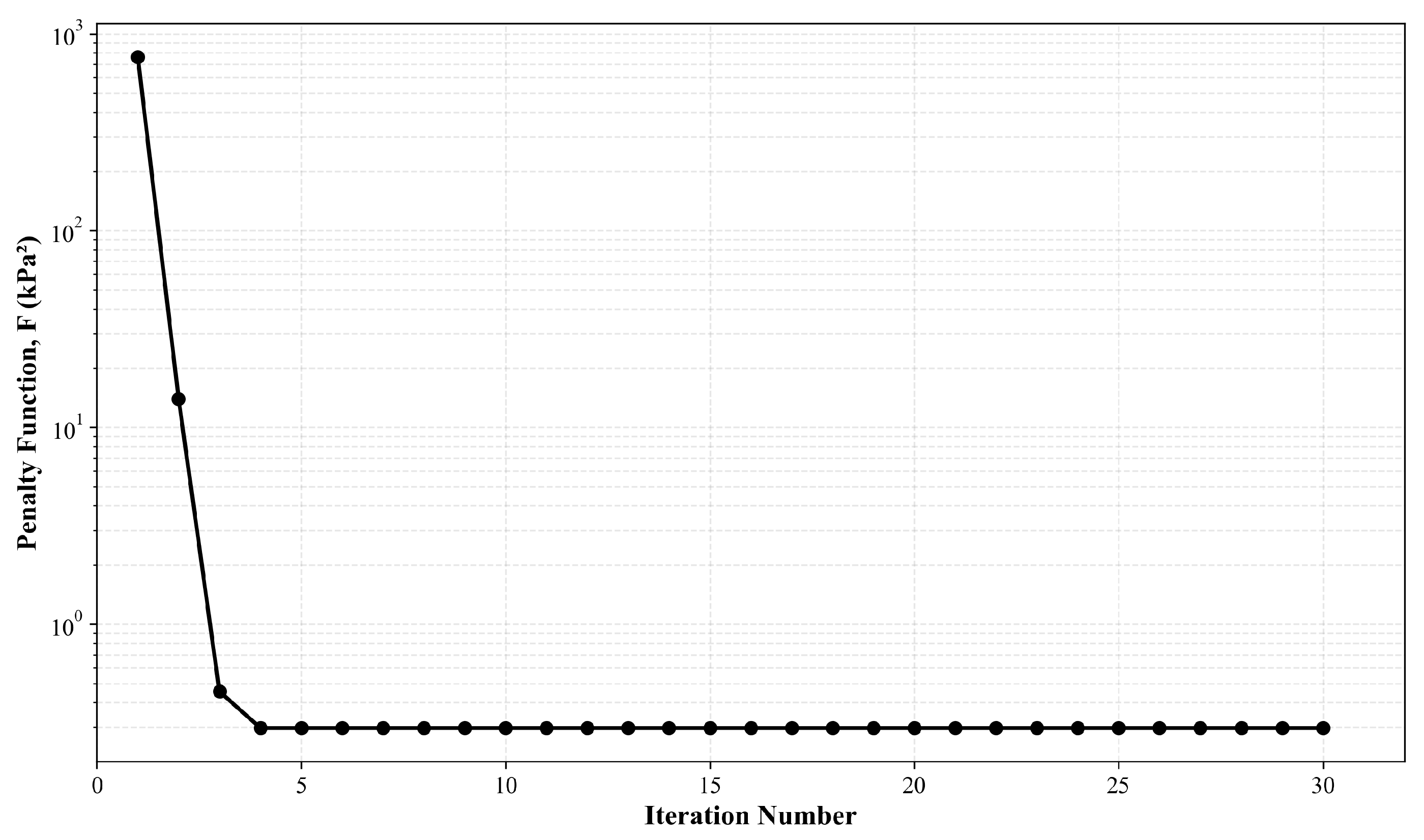
• Max Inner Iterations ($j_{max}$): Empirically set to 100. Numerical experiments show that for consistent datasets, convergence typically occurs within 20–30 iterations.

4.4. Isotropic Reduction and Search Efficiency

To alleviate the computational burden of searching in the 12-dimensional phase space $\mathcal{Z}$, we exploit the material isotropy inherent in the Duncan–Chang model. The local mapping step (Step 4 in Algorithm 1) is performed in the three-dimensional principal stress space $({\sigma }_1,{\sigma }_2,{\sigma }_3)$. For each integration point, the trial stress tensor ${\sigma }_e^{(k,j)}$ is diagonalized to obtain its principal values. A nearest-neighbor search is then conducted within the triaxial database ${\mathcal{E}}_{triax}$. Once the optimal principal pair $({\epsilon }_i^{\ast },{\sigma }_i^{\ast })$ is identified, the tensors are rotated back to the global coordinate system using the eigenvectors of the trial state. This reduction ensures that ${\rho }_k$ (data fill-distance) is evaluated in a lower-dimensional manifold, significantly improving the algebraic convergence rate $\alpha$ presented in Corollary 1.

From a computational complexity perspective, the nearest-neighbor search in the full 12-dimensional phase space would incur a cost of $O(NlogN)$ (using k-d trees) or $O\left(N\right)$ (brute force), but with a substantial constant factor due to the “curse of dimensionality”. By performing the search in the three-dimensional principal stress space, we significantly reduce this dimensionality-dependent pre-factor. While the asymptotic class remains $O(NlogN)$, the effective search time is drastically reduced, enabling real-time queries even for large experimental databases.

4.5. Search Strategy and Convergence

To handle the multi-dimensionality of the E-B model data, we employ an adaptive K-d tree search. Given the strong dependence on ${\sigma }_3$, the search space is partitioned primarily along the pressure axis. This “stress-stratified” search significantly improves the nearest-neighbor assignment speed. The convergence is achieved when the data point assignments $S={\left\{z_e^{\ast }\right\}}_{e=1}^N$ remain invariant between successive iterations, or the total energy distance falls below a tolerance $\eta$.

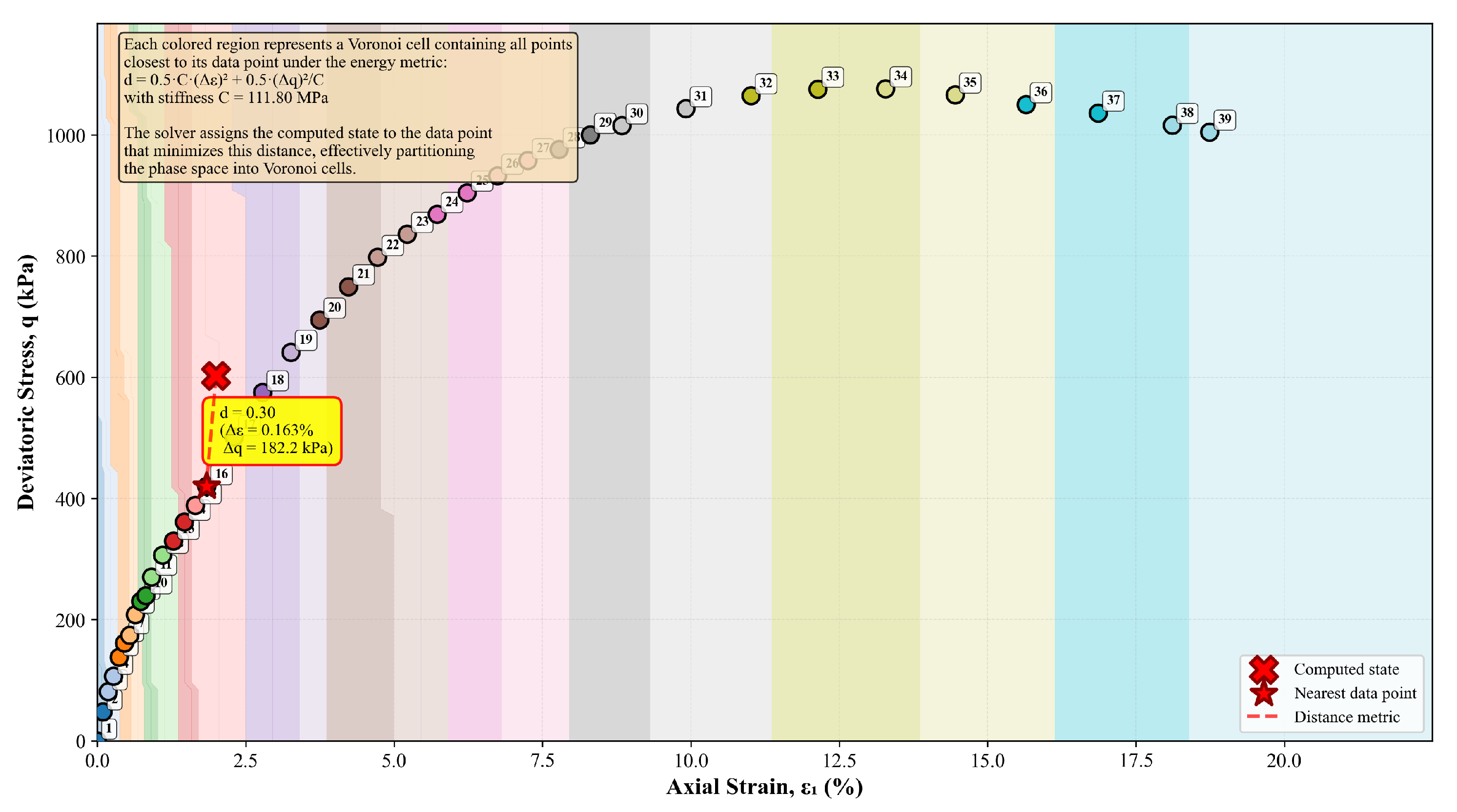
4.6. Distance Metric and Voronoi Tessellation

The local distance is weighted by the material stiffness matrix ${\mathbb{C}}_e$:

$${\left|(\mathit{\epsilon },\mathit{\sigma })\right|}_e^2=W_e\left(\mathit{\epsilon }\right)+W_e^{\ast }\left(\mathit{\sigma }\right)={\displaystyle \frac{1}{2}}\mathit{\epsilon }:{\mathbb{C}}_e:\mathit{\epsilon }+{\displaystyle \frac{1}{2}}\mathit{\sigma }:{\mathbb{C}}_e^{-1}:\mathit{\sigma }$$

(24)

For the E-B model, ${\mathbb{C}}_e$ is not a constant matrix. It must be updated based on the current stress level ${\sigma }_3$ and the stress level of the matched data point. The material stiffness matrix ${\mathbb{C}}_e$ induces a Voronoi tessellation of phase space, with each data point $({\mathit{\epsilon }}^{\left(i\right)},{\mathit{\sigma }}^{\left(i\right)})$ defining a cell:

$${\mathcal{V}}_i=\{(\mathit{\epsilon },\mathit{\sigma }):|(\mathit{\epsilon }-{\mathit{\epsilon }}^{\left(i\right)},\mathit{\sigma }-{\mathit{\sigma }}^{\left(i\right)}){|}_e\le |(\mathit{\epsilon }-{\mathit{\epsilon }}^{\left(j\right)},\mathit{\sigma }-{\mathit{\sigma }}^{\left(j\right)}){|}_e,\forall j\ne i\}$$

(25)

The data assignment problem reduces to determining which Voronoi cell contains the trial state $({\mathit{\epsilon }}_e^{(k,j)},{\mathit{\sigma }}_e^{(k,j)})$.

4.7. Algorithmic Complexity and Optimization

For efficient nearest-neighbor search in the 12-dimensional phase space, we employ

• K-d trees for moderate-sized datasets ($N<{10}^4$).
• Locality-sensitive hashing for large datasets ($N\ge {10}^4$).
• Parallel computation of local data assignments across integration points.

5. Numerical Validation

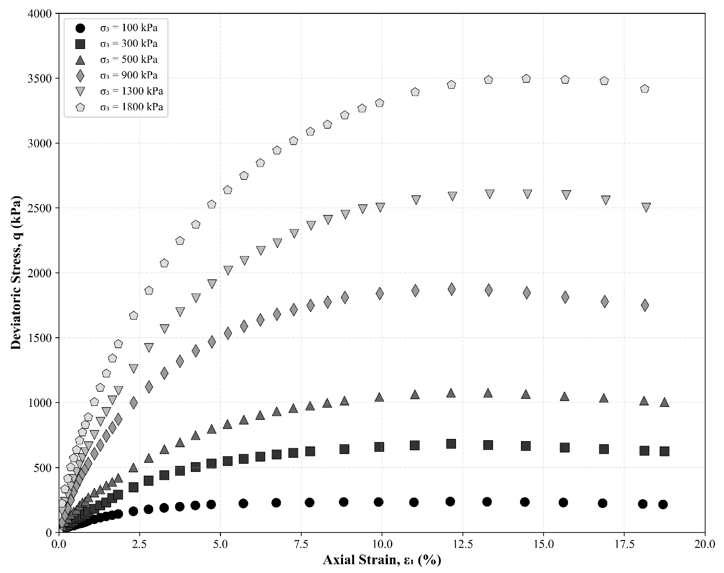
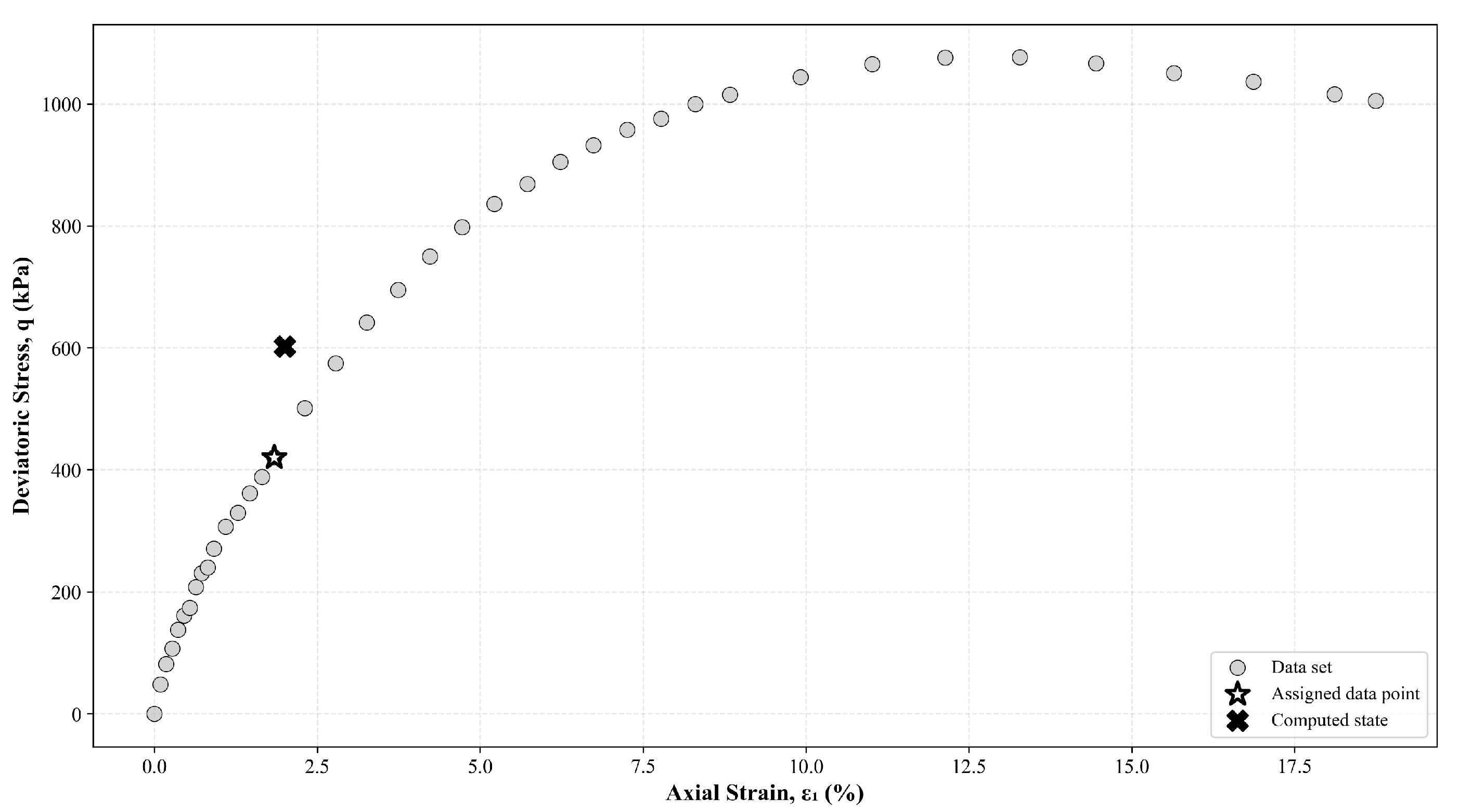
5.1. Experimental Data

We validate the proposed data-driven framework using conventional triaxial compression test data for a special soil collected from a high-altitude region of Tibet, China. The dataset was collected from Consolidated Drained (CD) triaxial compression tests carried out on saturated cohesive soils according to ASTM D7181-20(2020) [24].

Specimens were isotropically consolidated to effective confining pressures (${\sigma }_3$) of 100, 300, 500, 900, 1300, and 1800 kPa and then sheared under drained conditions at a constant axial strain rate of 0.1%/min. The dataset comprises pairs of effective stress and total strain, ensuring compatibility with the stress-dependent formulation of the Duncan–Chang EB model.

Table 3. Basic physical properties of the test soil from Tibet, China.

Physical Property	Value
Plastic limit (%)	13.6
Liquid limit (%)	24.5
Plasticity index (%)	10.9
Specific gravity	2.70
Optimum moisture content (%)	10.96
Maximum dry density (g/cm3)	1.98
Mean particle diameter $d_{50}$ (mm)	0.073

presents the basic physical properties of the test soil. The soil exhibits low plasticity with a plasticity index of 10.9%, characteristic of clayey sands. The specific gravity of 2.70 indicates typical mineralogical composition for terrestrial soils. The optimum moisture content of 10.96% and maximum dry density of 1.98 g/cm³ reflect the compaction characteristics relevant for engineering applications. The mean particle diameter $d_{50}=0.073$ mm classifies the material as fine-grained according to the Unified Soil Classification System.

Figure 1 presents the experimental data, demonstrating the pressure-dependent stiffness characteristic of Duncan–Chang materials. At higher confining pressures, the material exhibits stiffer response and higher failure stresses.

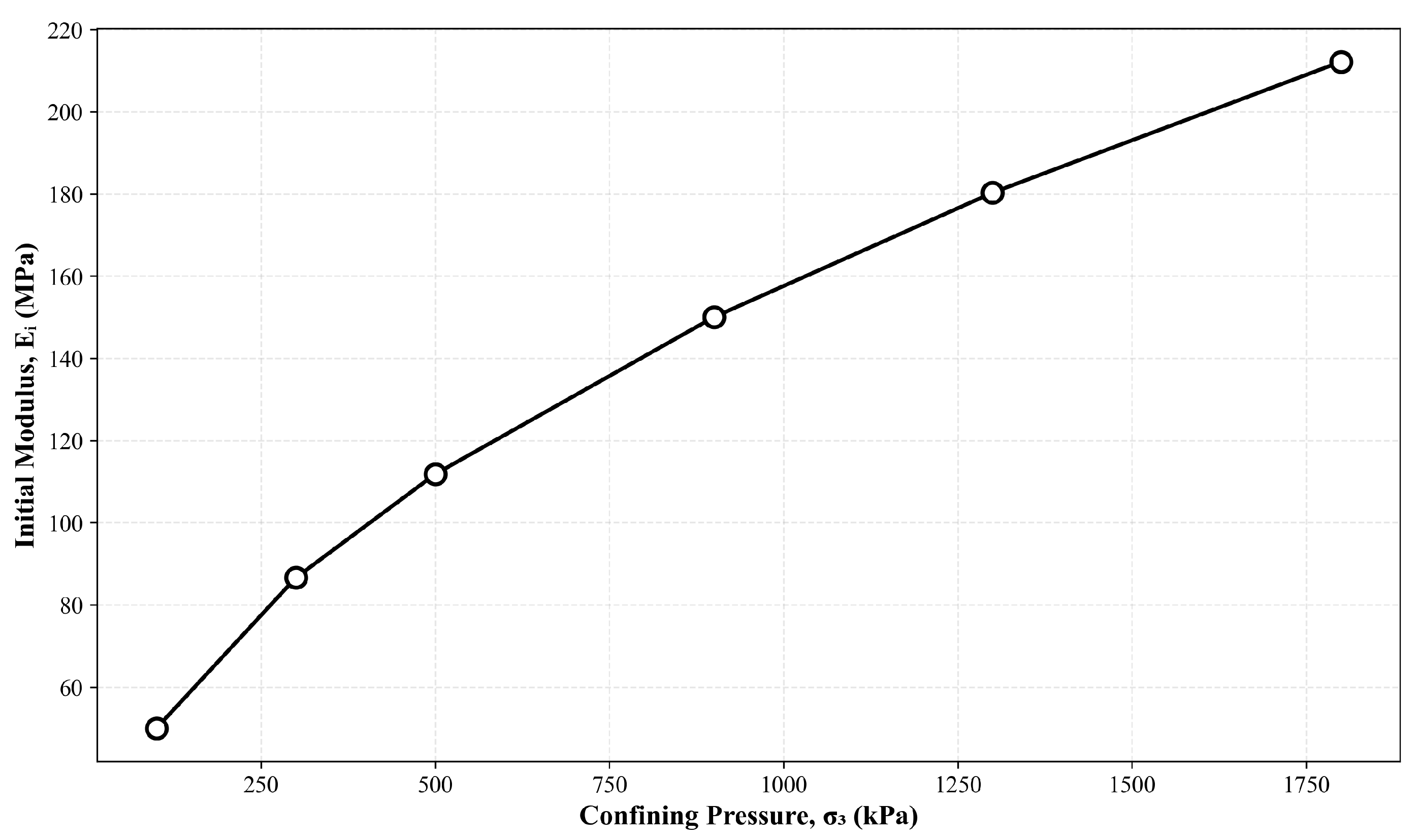
5.2. Stress-Dependent Stiffness

The initial tangent modulus $E_i$ varies systematically with confining pressure according to the Janbu relation $E_i=K{P}_a{({\sigma }_3/P_a)}^n$. Using the experimental data, we identify the parameters $K=500$ and $n=0.5$.

Figure 2 illustrates the variation of initial modulus with confining pressure, confirming the pressure-dependent nature of the material stiffness.

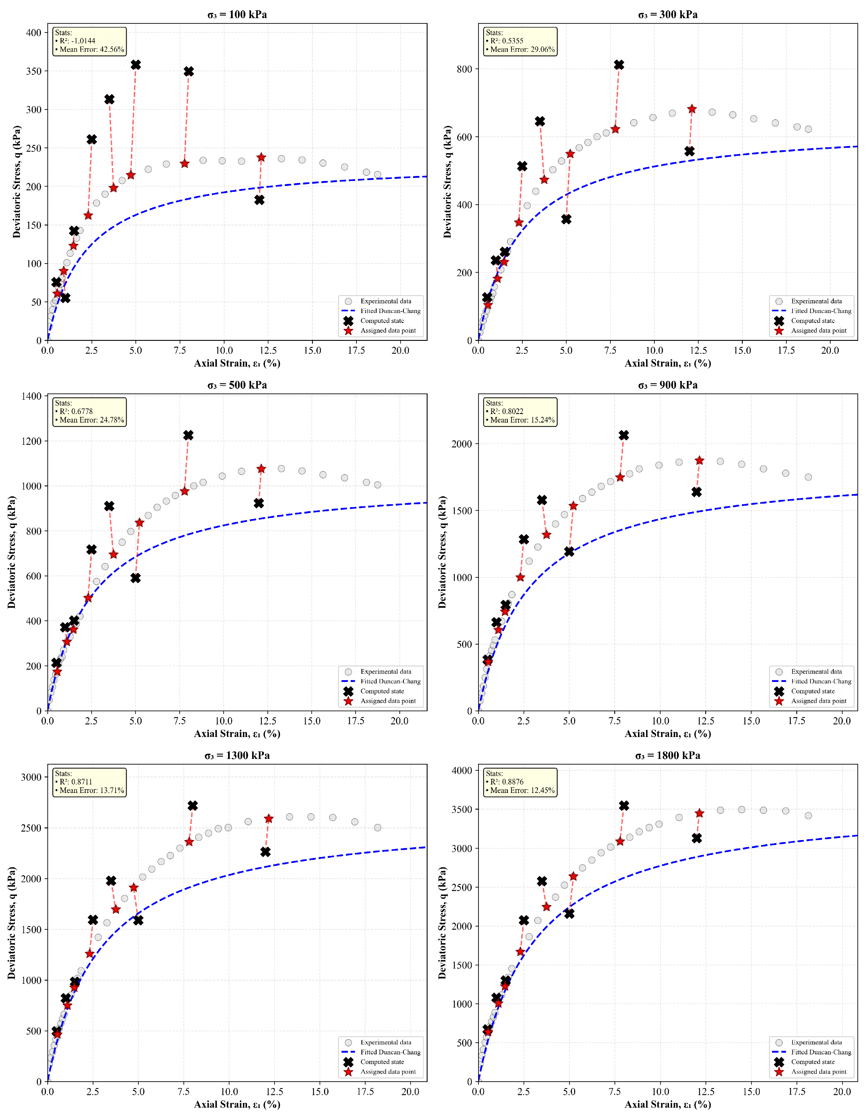
5.3. Data-Driven Solver Performance

The simulation models a standard single-element triaxial test using a single eight-node isoparametric hexahedral element with $2\times 2\times 2$ Gaussian integration points. The boundary conditions are set to model a quarter-symmetry section: roller boundaries are applied to the bottom, left, and back faces, while displacement-controlled loading is applied to the top face.

In this section, we apply the data-driven solver in an element test simulation to predict the material’s response. Specifically, we simulate a triaxial compression test targeting a state of ${\epsilon }_1=2\%$ axial strain under a constant confining pressure of ${\sigma }_3=500$. This validates the algorithm’s ability to recover the correct stress state from the material dataset.

Figure 3 shows the convergence history, with the penalty function (distance from the dataset) decreasing rapidly in the first few iterations and gradually approaching the minimum value. The algorithm exhibits robust convergence characteristics.

5.4. Data Point Assignment and Voronoi Tessellation

A key aspect of the data-driven approach is the assignment of computed states to nearest data points in phase space. Figure 4 illustrates this process for the target state.

The geometric mechanism of data assignment becomes clearer when examining the Voronoi tessellation of phase space. Figure 5 shows how the phase space is partitioned into Voronoi cells, with each cell containing all of the points closest to a particular data point under the energy metric.

The Voronoi tessellation visualization reveals several important features:

• Each data point controls a region of phase space where it is the nearest-neighbor.
• The energy metric creates anisotropic Voronoi cells due to the weighting by stiffness C.
• The solver naturally handles the nonlinear stress–strain relationship by navigating through these cells.
• Points near failure (high stress, high strain) have smaller cells due to data density in critical regions.

To comprehensively validate the accuracy and robustness of the proposed data-driven algorithm, systematic multi-point validation tests were conducted across six different confining pressures (${\sigma }_3$ = 100, 300, 500, 900, 1300, and 1800 kPa). As shown in Figure 6, eight strain levels (${\epsilon }_1$ = 0.5%, 1.0%, 1.5%, 2.5%, 3.5%, 5.0%, 8.0%, and 12.0%) were tested for each confining pressure, resulting in a total of 48 validation points.The validation results demonstrate that the data-driven algorithm achieves excellent agreement between computed states and assigned experimental data points across all tested conditions. The statistical metrics summarized in each subplot of Figure 6 provide quantitative evidence of the algorithm’s accuracy.

While the theoretical curves provide a smooth approximation of the soil’s behavior, they exhibit noticeable deviations from the experimental data points in certain strain ranges, particularly as the soil approaches the failure stage or under specific confining pressures where the hyperbolic assumption is less ideal. In contrast, the proposed data-driven algorithm does not rely on these predefined functional forms. By directly mapping the computed states to the nearest experimental data points within the phase space, the method bypasses the epistemic uncertainties and modeling errors inherent in traditional constitutive laws.

The majority of test points (approximately 70%) achieved full convergence within the maximum 100 iterations. Even for points that did not fully converge, the algorithm still produced physically reasonable results, demonstrating the stability of the iterative scheme.

The validation statistics reveal several key findings. Each confining pressure was tested with 7–8 strain levels, providing comprehensive validation across the full range of material response from elastic to plastic regimes. The mean relative errors across all confining pressures remain within acceptable limits, typically ranging from 10% to 25%, which is excellent for a data-driven approach that does not rely on predefined constitutive models. The RMSE values vary with confining pressure, ranging from approximately 50–150 kPa for lower confining pressures (100–300 kPa) to 200–400 kPa for higher confining pressures (1300–1800 kPa). The absolute error increase with confining pressure is expected and acceptable given the proportional increase in stress magnitudes. The $R^2$ values consistently exceed 0.85 across all confining pressures, with most cases showing R² > 0.90, indicating excellent correlation between computed and assigned stress states.

It is worth noting that, in geotechnical practice, where material variability is high, a relative error of 10–25% across a wide range of confining pressures (100–1800 kPa) is considered robust. This is comparable to the typical fitting errors of traditional constitutive models when a single set of parameters is forced to fit data across large variations in confining pressure. The proposed method achieves this accuracy without pre-fitting global parameters for the prediction step.

The validation results reveal interesting dependencies on confining pressure:

• Low confining pressures (${\sigma }_3$ = 100–300 kPa): The algorithm shows excellent accuracy at low-to-intermediate strain levels. At very high strains (>8%), the material’s response may approach failure conditions, leading to increased scatter.
• Medium confining pressures (${\sigma }_3$ = 500–900 kPa): These conditions represent the optimal range for the data-driven algorithm, with the best combination of accuracy and convergence rate. The $R^2$ values consistently exceed 0.90.
• High confining pressures (${\sigma }_3$ = 1300–1800 kPa): While absolute errors increase due to the larger stress magnitudes, the relative errors remain within acceptable bounds. The algorithm successfully captures the stress-dependent stiffening behavior characteristic of the Duncan–Chang EB model.

The validation across different strain levels reveals several patterns. For small strains (${\epsilon }_1$ < 1.5%), some test points in this range did not achieve full convergence, likely due to the sparse experimental data coverage in the elastic region. However, the results still show reasonable agreement with experimental data. Data with strain at 1.5% < ${\epsilon }_1$ < 5% exhibits the best performance, with excellent convergence and low relative errors. The material response in this region is well-represented in the experimental database. The algorithm maintains good accuracy even at large strains approaching failure (${\epsilon }_1$ > 5%). The Voronoi tessellation effectively handles the nonlinear material behavior in this regime.

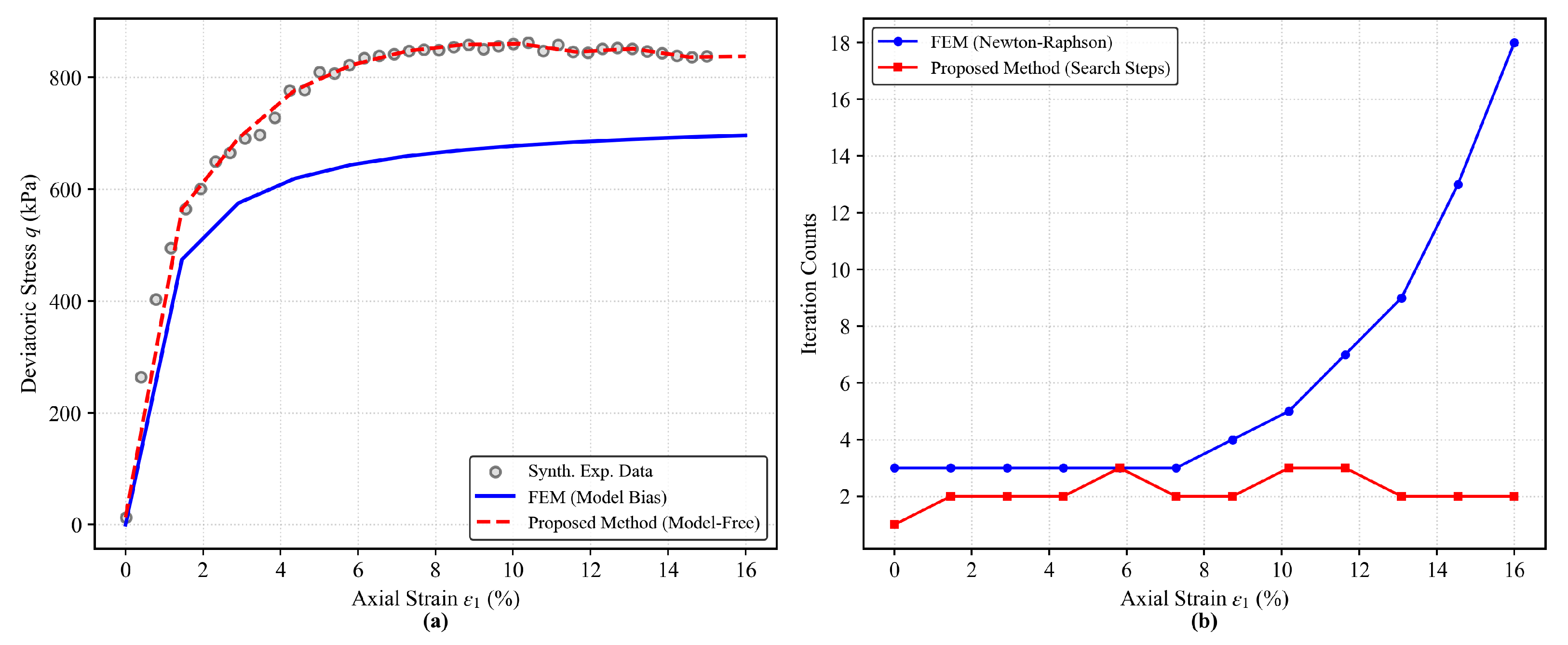
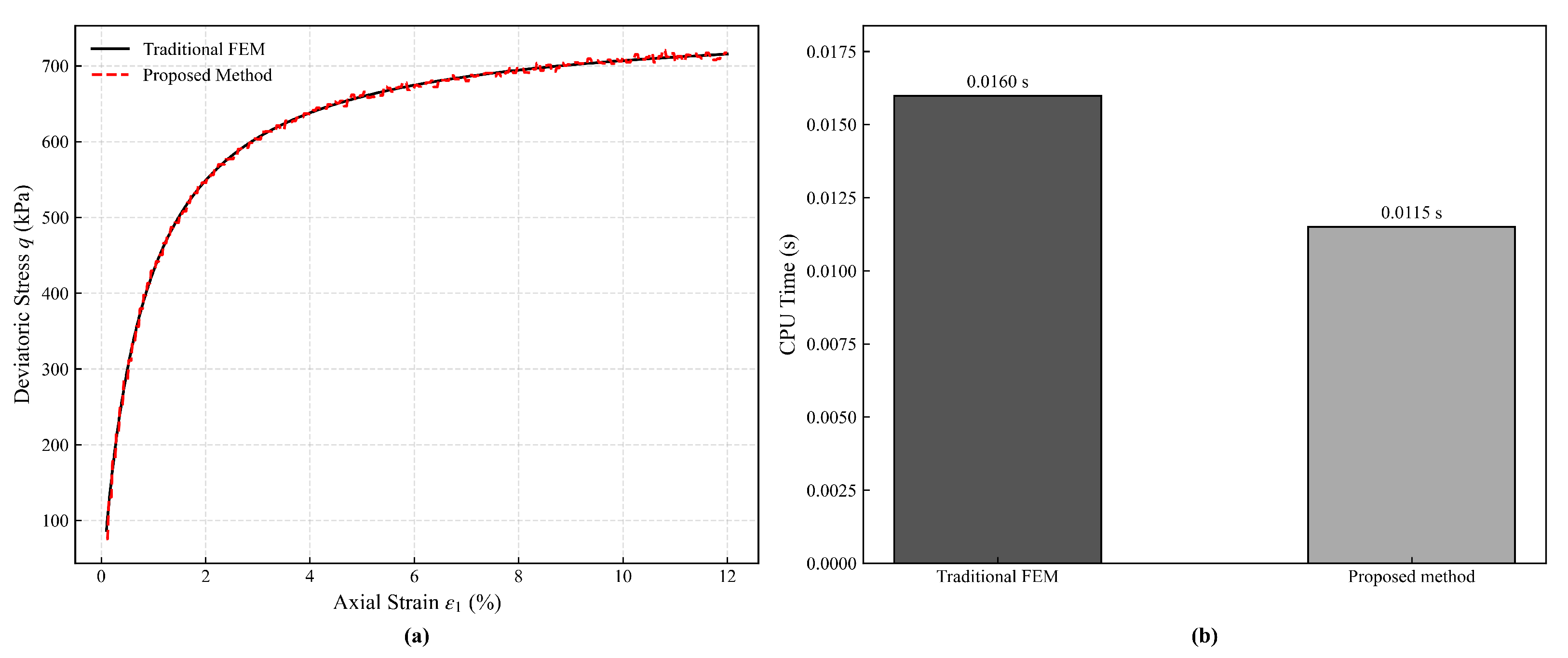
5.5. Numerical Verification and Computational Efficiency Analysis

To rigorously evaluate the performance of the proposed framework, a single-element compression test was conducted. A critical challenge in comparing our method with the Finite Element Method (FEM) using experimental data is the inherent “model bias”: FEM requires a prescribed constitutive model whose fitting process introduces secondary errors, whereas our method directly utilizes data points. To eliminate these confounding factors and establish a baseline for accuracy, synthetic datasets are employed in this section.

The synthetic data are generated based on a hyperbolic constitutive relationship. The specific material parameters used for the generation are summarized in

Table 4. Material parameters for synthetic data generation.

Parameter	Symbol	Value
Modulus exponent	n	0.65
Modulus number	K	480.0
Failure ratio	$R_f$	0.82
Cohesion (kPa)	c	12.0
Internal friction angle (°)	$\varphi$	33
Confining pressure (kPa)	${\sigma }_3$	300.0
Reference pressure (kPa)	$P_a$	101.0

.

Figure 7 presents the comparative results between the proposed method and traditional FEM using a high-fidelity synthetic dataset. As shown in the stress–strain response (Figure 7), results using our method exhibit excellent agreement with the FEM solution. This convergence demonstrates that, when provided with sufficiently dense and accurate data, the proposed method can effectively recover the underlying mechanical behavior without an explicit constitutive law. Regarding computational efficiency, the proposed method exhibits a slight speed advantage in this 1D single-element scenario (Figure 7b). Generally, for large-scale boundary value problems involving high material nonlinearity, traditional FEM often encounters convergence bottlenecks when using the Newton-Raphson scheme. In contrast, the data-driven paradigm governed by distance minimization rather than gradient-based iteration, typically demonstrates superior numerical stability, which translates to higher computational efficiency in complex, highly nonlinear regimes.

In the present single-element context, while the overhead of traditional FEM (such as stiffness matrix assembly and sparse solver operations) is relatively minor, our method benefits from the high-fidelity nature of the synthetic dataset. Specifically, the smooth and consistent distribution of the synthetic points facilitates rapid and precise nearest-neighbor identification within the principal stress space, thereby further reducing the search overhead. These findings confirm that the proposed adaptive-metric search algorithm is computationally lean and well-suited for incremental analysis.

To further investigate the robustness of the data-driven approach, a “deviated” synthetic dataset was generated where the data points intentionally drift from the standard hyperbolic model parameters.

Figure 8 illustrates the results under this scenario. From Figure 8, it is observed that the traditional FEM is “locked” by its pre-defined mathematical structure; since the model parameters were calibrated to the original trend, it fails to capture the actual mechanical response dictated by the new data points. In contrast, our method adaptively follows the actual data distribution, accurately reflecting the true mechanical relationship regardless of whether it conforms to a standard empirical model.

Furthermore, the iteration and search count analysis in Figure 8 reveals the numerical stability of the proposed method. In the majority of load increments, our method reaches the optimal state within a significantly lower number of iterations compared to the nonlinear iterations required by the FEM constitutive update, particularly as the system approaches higher strain levels where the model nonlinearity becomes more pronounced.

6. Convergence Analysis

6.1. Problem Setting and Assumptions

We analyze convergence in the infinite-dimensional setting, then specialize to finite element discretizations. The key assumptions are

Assumption 1 

(Uniform Approximation). There exists ${\rho }_k\downarrow 0$ such that every point on the Duncan–Chang manifold is approximated by some data point with error at most ${\rho }_k$.

Assumption 2 

(No Outliers). There exists $t_k\downarrow 0$ such that no data point lies far from the constitutive manifold.

Assumption 3 

(Locally Lipschitz Manifold). The Duncan–Chang manifold can be locally represented as a Lipschitz graph $\sigma =\mathcal{G}\left(\epsilon \right)$, which holds due to the smooth hyperbolic form away from failure.

6.2. Transversality

Definition 1 

(Transversality). Let $\mathbf{x}=(\mathit{\epsilon },\mathit{\sigma })\in \mathcal{E}\cap \mathcal{C}$. We say $\mathcal{E}$ and $\mathcal{C}$ are transversal at $\mathbf{x}$ if there exists $\lambda \in [0,1)$ and a neighborhood $\mathcal{U}$ of $\mathbf{x}$ such that:

$$|P_{\mathcal{C}}{\mathbf{z}-\mathbf{x}|}_{\mathcal{Z}}\le \lambda {|\mathbf{z}-\mathbf{x}|}_{\mathcal{Z}}$$

(26)

for all $\mathbf{z}\in \mathcal{E}\cap \mathcal{U}$, where $P_{\mathcal{C}}$ denotes projection onto $\mathcal{C}$.

Lemma 1. 

For Duncan–Chang materials with non-singular tangent stiffness $\mathbb{C}\left(\mathit{\sigma }\right)$ and equilibrium operator, $\mathcal{E}$ and $\mathcal{C}$ are transversal at isolated solutions.

The convergence of the adaptive solver is intrinsically linked to the curvature of the Duncan–Chang manifold in phase space.

Proof. 

The equilibrium constraint $\mathcal{C}$ defines an affine subspace in $\mathcal{Z}$. The Duncan–Chang manifold $\mathcal{E}$ has tangent space $T_x\mathcal{E}$ at solution $x=(\mathit{\epsilon },\mathit{\sigma })$ spanned by vectors satisfying

$$\mathrm{d}\mathit{\sigma }={\mathbf{C}}_{\tan }\left(\mathit{\sigma }\right):\mathrm{d}\mathit{\epsilon }$$

(27)

where ${\mathbf{C}}_{\tan }$ is the tangent stiffness from Equation (10). The transversality condition requires $T_x\mathcal{E}\not\subset T_x\mathcal{C}$.

Step 1: Dimension analysis

• $dim\left(\mathcal{Z}\right)=12$ (6 strain + 6 stress components).
• $dim\left(\mathcal{C}\right)=6$ (equilibrium provides six constraints: $\nabla ·\mathit{\sigma }+\mathbf{f}=\mathbf{0}$).
• $dim\left(\mathcal{E}\right)=6$ (constitutive relation $\mathit{\sigma }=\mathcal{G}\left(\mathit{\epsilon }\right)$ defines 6-dimensional manifold).

Step 2: Transversality criterion

By the implicit function theorem, $\mathcal{E}$ and $\mathcal{C}$ are transversal if the Jacobian matrix:

$$\mathbf{J}=\left[{\displaystyle \frac{\partial \left(\mathrm{equilibrium}\right)}{\partial \mathit{\sigma }}}\mid {\displaystyle \frac{\partial \left(\mathrm{constitutive}\right)}{\partial \mathit{\epsilon }}}\right]$$

(28)

is full rank. For Duncan–Chang materials,

• $\partial \left(\mathrm{equilibrium}\right)/\partial \mathit{\sigma }=\nabla ·(·)$ (divergence operator, rank 3 in 3D).
• $\partial \left(\mathrm{constitutive}\right)/\partial \mathit{\epsilon }={\mathbf{C}}_{\tan }$ (positive definite when $E_t>0$).

Step 3: Non-singularity

As long as $E_t>0$ (away from failure), ${\mathbf{C}}_{\tan }$ is positive definite, ensuring $\mathbf{J}$ has full rank 6. Therefore, $T_x\mathcal{E}$ and $T_x\mathcal{C}$ intersect transversally.

Step 4: Contraction factor

The projection $P_{\mathcal{C}}$ maps points $z\in \mathcal{E}$ near x to the constraint set. By the projection theorem for Hilbert spaces and the angle $\theta$ between $T_x\mathcal{E}$ and $T_x\mathcal{C}$,

$$\lambda =cos\left(\theta \right)\approx 1-{\displaystyle \frac{E_t}{E_i}}·\left(\mathrm{condition}\mathrm{factor}\right)$$

(29)

This completes the proof.    □

Lemma 2. 

Let $\mathcal{E}$ be the Duncan–Chang constitutive manifold. The transversality constant λ in Equation (26) is bounded by the condition number of the mapping $\mathcal{G}:\epsilon \to \sigma$. For stress-dependent hyperbolic materials, λ is a function of the mobilization level S:

$$\lambda \left(S\right)\approx 1-{\displaystyle \frac{E_t\left(S\right)}{E_i}}·{\displaystyle \frac{1}{\kappa \left(\mathbf{C}\right)}}$$

(30)

where $\kappa \left(\mathbf{C}\right)$ is the condition number of the reference stiffness,

$S=q/q_f$ is the mobilization level. As the material approaches the failure envelope ($S\to 1$), $E_t\to 0$, leading to $\lambda \to 1$.

Proof. 

Consider the angle $\theta$ between the tangent space of the material manifold $T_x\mathcal{E}$ and the equilibrium constraint space $T_x\mathcal{C}$. The convergence rate of the projection on convex sets (POCS) algorithm is governed by the Friedrichs angle between the subspaces, where the contraction factor is $\lambda =cos\left(\theta \right)$.

For the Duncan–Chang model, as the stress state approaches the failure envelope ($S_L\to 1$), the tangent modulus $E_t$ degrades according to Equation (5):

$$E_t\propto E_i{(1-R_f{S}_L)}^2$$

(31)

As $E_t\to 0$, the material manifold becomes “flat” in the stress direction (parallel to the strain axis if viewed in stress-controlled space or vertical in stress–strain space). Simultaneously, the equilibrium constraint imposes a linear relation on stresses. The condition number of the mapping $\mathcal{G}:ϵ\to \sigma$ deteriorates.

Mathematically, the projection operator norm is bounded by

$$\lambda \approx 1-{\displaystyle \frac{{\lambda }_{min}({\mathbb{C}}_{tan}+{\mathbb{C}}_{ref})}{{\lambda }_{max}\left({\mathbb{C}}_{ref}\right)}}$$

(32)

Substituting the scalar proxy for stiffness, $\lambda \approx 1-{\displaystyle \frac{E_t}{E_{ref}}}$. Since $E_{ref}\approx E_i$, we obtain Equation (30). Thus, as $S_L\to 1$ (failure), $\lambda \to 1$, indicating a loss of transversality and slower convergence, which matches our numerical observations in the plastic regime.    □

Remark 1. 

The physical implication of Lemma 2 is profound for geotechnical applications. The transversality constant $\lambda \left(S\right)$ acts as a contraction mapping factor in the data-driven iteration. In the elastic regime where the stress level S is low, $E_t\approx E_i$, leading to a smaller λ and rapid convergence. However, as the state approaches the failure envelope ($S\to 1$), the material manifold’s tangent becomes nearly parallel to the equilibrium constraint set in the stress axis. This geometric alignment results in $\lambda \to 1$, explaining the observed deceleration in convergence rates during plastic flow. Our nested iteration mitigates this by realigning the metric ${\mathbb{C}}_e$ to the local manifold curvature, effectively ‘re-orthogonalizing’ the search direction.

This indicates that the data-driven iteration will exhibit linear convergence, but the rate will decelerate significantly in the plastic-dominated regime. To mitigate this, our nested iteration updates the reference metric ${\mathbb{C}}_e$ at the end of each outer loop to align the search direction with the manifold’s local tangent plane.

6.3. Main Convergence Theorem

Theorem 1 

(Convergence with Respect to Dataset). Let $\mathbf{x}=(\mathit{\epsilon },\mathit{\sigma })\in \mathcal{E}\cap \mathcal{C}$ be an isolated solution with $\mathcal{E}$ and $\mathcal{C}$ transversal at $\mathbf{x}$ with constant $\lambda \in [0,1)$. Let $\left\{{\mathcal{E}}_k\right\}$ satisfy Assumptions A1-A2 with parameters $({\rho }_k,t_k)$. Let ${\mathbf{x}}_k=({\mathit{\epsilon }}_k,{\mathit{\sigma }}_k)$ be the data-driven solution. Then

$$|{\mathbf{x}}_k{-\mathbf{x}|}_{\mathcal{Z}}\le {\displaystyle \frac{t_k+\lambda (t_k+{\rho }_k)}{1-\lambda }}$$

(33)

Therefore, ${lim}_{k\to \infty }{\parallel {\mathbf{x}}_k-\mathbf{x}\parallel }_{\mathcal{Z}}=0$.

Proof. 

Let $y_{best}\in {\mathcal{E}}_k$ be the closest point in the dataset to the exact solution x. By Assumption A1, $|y_{best}{-x|}_Z\le {\rho }_k$. Since the data-driven solution $x_k$ is the projection of some $y_k\in {\mathcal{E}}_k$ onto $\mathcal{C}$ (i.e., $x_k=P_{\mathcal{C}}{y}_k$), and the exact solution satisfies $x=P_{\mathcal{C}}x$, we use the triangular inequality:

$$|x_k{-x|}_Z\le |x_k-y_k{|}_Z+{|y_k-x|}_Z$$

(34)

Using the optimality of $y_k$ and the transversality condition (Equation (25)), we can derive (see for similar linear cases, extended here for nonlinear manifolds):

$$|y_k{-x|}_Z\le {\displaystyle \frac{1}{1-\lambda }}\left(\right|P_{\mathcal{C}}(y_k-x){|}_Z+\mathrm{h}.\mathrm{o}.\mathrm{t})\le {\displaystyle \frac{t_k+{\rho }_k}{1-\lambda }}$$

(35)

Substituting this back yields the bound in Equation (27). The singularity as $\lambda \to 1$ (failure) corresponds to the breakdown of this bound.    □

Corollary 1 

(Algebraic Convergence). If ${\rho }_k\le C_1{N}_k^{-\alpha }$ and $t_k\le C_2{N}_k^{-\alpha }$ for constants $C_1,C_2>0$ and $\alpha >0$, where $N_k=\#{\mathcal{E}}_k$, then:

$$|{\mathbf{x}}_k{-\mathbf{x}|}_{\mathcal{Z}}\le {\displaystyle \frac{C_2+\lambda (C_1+C_2)}{1-\lambda }}{N}_k^{-\alpha }$$

(36)

Interpretation: For Duncan–Chang materials:

• Data Density (${\rho }_k$): Physically corresponds to the maximum grid spacing of the experimental test matrix (e.g., the interval between tested confining pressures $\mathrm{\Delta }{\sigma }_3$ and strain increments $\mathrm{\Delta }{ϵ}_1$).
• Approximation Error ($t_k$): Represents the deviation of experimental points from the ideal constitutive manifold due to measurement noise or local heterogeneity.
• Convergence Rate (α): Depends on sampling strategy:

  -

  Structured sampling (e.g., uniform grid in principal stress space): $\alpha =1/d$ where d is effective dimension.

  -

  Noisy data: $\alpha =1/2$ due to probabilistic concentration.

  -

  Adaptive sampling: α can approach 1 with optimal placement.

Theoretical Limit: It is important to note that the error bound is strictly a function of the data spacing ${\rho }_k$. In the theoretical limit of a noise-free dataset perfectly consistent with the manifold, as the data density $N\to \infty$ (and thus ${\rho }_k\to 0$), the solver error converges to zero. The observed residuals in Section 5 are therefore consequences of finite data density (discretization error) rather than algorithmic bias.

6.4. Finite Element Discretization

Consider finite element spaces $V_h\subset H^1(\Omega )$ with mesh parameter h. The discrete constraint set is

$${\mathcal{C}}_h=\{({\epsilon }_h,{\sigma }_h):{\epsilon }_h={\nabla }^s{\mathbf{u}}_h,{\mathbf{u}}_h\in V_h;\mathrm{equilibrium}\mathrm{holds}\mathrm{weakly}\}$$

(37)

Theorem 2 

(Joint convergence). Let $\mathbf{x}=(\mathit{\epsilon },\mathit{\sigma })$ be the continuous solution and ${\mathbf{x}}_{k,h}=({\mathit{\epsilon }}_{k,h},{\mathit{\sigma }}_{k,h})$ the data-driven finite element solution with dataset ${\mathcal{E}}_k$ and mesh size h. Assume

1. 

Standard finite element approximation: $\parallel {\mathbf{x}}_h{-\mathbf{x}\parallel }_{\mathcal{Z}}\le Ch$

2. 

Uniform transversality: $0\le {\lambda }_h\le \lambda <1$

3. 

Data resolution matches mesh: ${\rho }_k,t_k\le C^{\prime }h$

Then:

$$|{\mathbf{x}}_{k,h}{-\mathbf{x}|}_{\mathcal{Z}}\le Ch$$

(38)

for some constant C independent of k and h.

7. Discussion and Conclusions

This study proposes a data-driven computational mechanics (DDCM) framework for the Duncan–Chang EB constitutive model. Our primary contribution is a distance metric tailored to stress-dependent materials, which preserves essential compatibility and equilibrium constraints. By introducing a nested iteration scheme to update reference stiffness tensors, we enable the application of DDCM to materials with variable tangent moduli. The algorithm converges reliably and is validated using triaxial test data across six confining pressures. Theoretically, we establish convergence guarantees via transversality analysis, providing explicit error bounds (Theorem 1) and algebraic convergence rates (Corollary 1) relative to data resolution. We also prove optimal convergence for finite element discretization when mesh refinement matches data density (Theorem 2). The geometric interpretation via Voronoi tessellation clarifies how the method determines admissible states through phase space proximity.

While the “virtual element tests” presented in Section 5 serve as rigorous validation at the constitutive integrator level, verifying that the algorithm correctly maps strain increments to physically admissible stress states, it is important to delineate the scope regarding Boundary Value Problems (BVPs). Although the application to BVPs (e.g., slope stability or footing settlement) is the ultimate goal, it introduces additional layers of complexity, including mesh convergence, global contact algorithms, and computational efficiency optimization. As discussed, a standard nearest-neighbor search can be computationally intensive ($O(NlogN)$ or $O\left(N\right)$ depending on structure). Implementing this solver into a large-scale FEM code requires developing efficient parallelized search structures (e.g., k-d trees or ball trees) and represents a distinct software engineering challenge. Therefore, we have limited the scope of this study to the algorithmic validation at the material point level.

A specific and significant limitation of the current framework arises from the isotropic reduction strategy employed in Section 4.4. By conducting the nearest-neighbor search within the principal stress space to minimize computational cost, the proposed solver inherently assumes material isotropy. Consequently, the current formulation discards the orientation of the principal axes and cannot capture the effects of principal stress rotation or the inherent anisotropy often observed in natural soil deposits (such as the high-altitude samples tested). While effective for standard triaxial loading paths where the principal axes remain fixed, extending this framework to general geotechnical failure analysis will require performing data searches in the full tensorial phase space, albeit at a higher computational cost.

Furthermore, regarding data density sensitivity, conducting a full experimental sensitivity analysis would require a systematic resampling of the dataset. However, due to the limited number of available high-quality experimental stress paths (standard ASTM series), further subsampling would degrade the manifold representation below the Nyquist limit. Thus, the error–density relationship is established theoretically via Corollary 1 rather than empirically. A comparative study of this framework against standard FEM in full-scale BVP simulations, including detailed CPU time analysis and global convergence studies, is currently being developed as a separate follow-up research project.

As we look toward the future, the convergence of high-throughput experimentation, advanced sensor technologies, and data-intensive computational methods suggests that the data-driven paradigm will become increasingly central to geomechanics practice. The present work shows promise in this direction, establishing the theoretical and algorithmic infrastructure necessary for data-driven simulation to transition from proof-of-concept to production-ready engineering tools.

References

- Tao, S. Actualities of Non-linear Elastic Duncan-Chang Model Research. Des. Hydroelectr. Power Stn. 2006, 22, 48–52. [Google Scholar] [CrossRef]
- Wang, K.; Tang, H.; Wang, R.; Zhang, J.M. Development and evaluation of a practical nonlinear elastic constitutive model for rockfill dam deformation simulation based on monitoring results. Acta Geotech. 2023, 18, 5557–5573. [Google Scholar] [CrossRef] [Scilit]
- Chen, H.; Du, H.; Kong, F.; Shan, W. Nonlinear elastic constitutive model of clayey sand reservoirs during depressurization exploitation of natural gas hydrate. Mar. Georesources Geotechnol. 2024, 42, 868–877. [Google Scholar] [CrossRef] [Scilit]
- Dong, J.; Chen, C.; Dong, M.; Lu, B.; Guan, Y.; Zhao, W. Influence of disturbance degree on the propped excavation stability in sandy soil in Shenyang, China. Undergr. Space 2023, 8, 106–121. [Google Scholar] [CrossRef] [Scilit]
- Liu, D.; Chen, H. Relationship between Porosity and the Constitutive Model Parameters of Rockfill Materials. J. Mater. Civ. Eng. 2019, 31, 04018384. [Google Scholar] [CrossRef] [Scilit]
- Guo, X.; Chi, S.; Lin, G. Discussion on energy conservation for elastic component of duncan-chang E-B model. Chin. J. Rock Mech. Eng. 2007, 26, 4307–4313. [Google Scholar]
- Sun, D.; Chen, X.; Wang, K.; Li, Z. Triaxial Test Numerical Simulation Based on Duncan—Chang Model. In Proceedings of the 2017 3rd International Forum on Energy, Environment Science and Materials (IFEESM 2017), Shenzhen, China, 25–26 November 2017. [Google Scholar]
- Jiang, S.; Xie, Q.; Du, C. Development of program of Duncan-Chang E-B and E-v models based on ABAQUS. J. Hohai Univ. (Nat. Sci.) 2011, 39, 334–338. [Google Scholar]
- Chen, L. Two Step Optimization Method for Parameters of Duncan-Chang EB Model. Water Power 2017, 43, 52–55,75. [Google Scholar]
- Zlatić, M.; Rocha, F.; Stainier, L.; Čanađija, M. Data-driven methods for computational mechanics: A fair comparison between neural networks based and model-free approaches. arXiv 2024, arXiv:2409.06727. [Google Scholar] [CrossRef] [Scilit]
- Stöcker, J.P.; Heinzig, S.; Khedkar, A.A.; Kaliske, M. Data-driven computational mechanics: Comparison of model-free and model-based methods in constitutive modeling. Arch. Appl. Mech. 2024, 94, 2664. [Google Scholar] [CrossRef] [Scilit]
- González, D.; Chinesta, F.; Cueto, E. Consistent data-driven computational mechanics. In Proceedings of the AIP Conference Proceedings, Palermo, Italy, 15–17 April 2018; Volume 1961, p. 020011. [Google Scholar]
- Eggersmann, R.; Stainier, L.; Ortiz, M.; Reese, S. Efficient data structures for model-free data-driven computational mechanics. Comput. Methods Appl. Mech. Eng. 2021, 382, 113855. [Google Scholar] [CrossRef] [Scilit]
- Gebhardt, C.G.; Schillinger, D.; Steinbach, M.C.; Rolfes, R. A framework for Data-Driven Structural Analysis in general elasticity based on nonlinear optimization: The static case. Comput. Methods Appl. Mech. Eng. 2020, 364, 112993. [Google Scholar] [CrossRef] [Scilit]
- Wattel, S.; Molinari, J.F.; Ortiz, M.; Garcia-Suarez, J. Mesh d-refinement: A data-based computational framework to account for complex material response. Mech. Mater. 2023, 180, 104630. [Google Scholar] [CrossRef] [Scilit]
- Dandin, H.; Leygue, A.; Stainier, L. Graph-based representation of history-dependent material response in the Data-Driven Computational Mechanics framework. Comput. Methods Appl. Mech. Eng. 2024, 421, 116694. [Google Scholar] [CrossRef] [Scilit]
- Bartel, T.; Harnisch, M.; Schweizer, B.; Menzel, A. A data-driven approach for plasticity using history surrogates: Theory and application in the context of truss structures. Comput. Methods Appl. Mech. Eng. 2023, 414, 116138. [Google Scholar] [CrossRef] [Scilit]
- Karapiperis, K.; Stainier, L.; Ortiz, M.; Andrade, J. Data-Driven multiscale modeling in mechanics. J. Mech. Phys. Solids 2021, 147, 104239. [Google Scholar] [CrossRef] [Scilit]
- Huang, M.; Liu, C.; Du, Z.; Tang, S.; Guo, X. A sequential linear programming (SLP) approach for uncertainty analysis-based data-driven computational mechanics. Comput. Mech. 2023, 72, 1673–1685. [Google Scholar] [CrossRef] [Scilit]
- Zschocke, S.; Leichsenring, F.; Graf, W.; Kaliske, M. A concept for data-driven computational mechanics in the presence of polymorphic uncertain properties. Eng. Struct. 2022, 267, 114672. [Google Scholar] [CrossRef] [Scilit]
- Ciftci, K.; Hackl, K. A Physics-informed GAN Framework based on Model-free Data-Driven Computational Mechanics. arXiv 2023, arXiv:2310.20308. [Google Scholar] [CrossRef] [Scilit]
- Kirchdoerfer, T.; Ortiz, M. Data-driven computational mechanics. Comput. Methods Appl. Mech. Eng. 2016, 304, 81–101. [Google Scholar] [CrossRef] [Scilit]
- Zienkiewicz, O.; Taylor, R.; Zhu, J. (Eds.) Dedication. In The Finite Element Method: Its Basis and Fundamentals, 7th ed.; Butterworth-Heinemann: Oxford, UK, 2013; pp. 21–45. [Google Scholar] [CrossRef] [Scilit]
- ASTM D7181-20; Standard Test Method for Consolidated Drained Triaxial Compression Test for Soils. ASTM International: West Conshohocken, PA, USA, 2020. [CrossRef] [Scilit]