The Paradox Between Correlations and Sign Predictability

Abstract

This paper uncovers a paradoxical disconnect between two widely used metrics for forecast evaluation: Mean Directional Accuracy (MDA) and the correlation between the forecast and the target variable. We show that a forecast that is more strongly correlated with the target may deliver poorer sign predictions than a less correlated alternative. Within a Gaussian framework, we derive analytical expressions showing that directional accuracy depends not only on correlation but also on the standardized means of both the forecast and the target variable. As a consequence, higher correlation does not guarantee superior sign predictability. We illustrate this paradox through analytical examples and derive formal conditions under which it cannot arise. Interestingly, we show that when forecasts are efficient, the MDA Paradox is impossible. Finally, we present an empirical application from the exchange rate literature that demonstrates the practical relevance of our results.

1. Introduction

Forecast evaluation relies on a variety of statistical metrics, each capturing different aspects of predictive quality. While Mean Squared Prediction Error (MSPE) is the most commonly used criterion, other measures, such as Mean Absolute Error (MAE), correlations between forecasts and the target variable, and Mean Directional Accuracy (MDA), are also widely employed (MDA is also known as hit-rate, success rate or sign agreement ratio, and it is considered in many articles studying predictability, including [1,2,3,4,5,6], among many others). MDA, in particular, measures a forecast’s ability to correctly anticipate the direction of change in the target variable, making it especially relevant for investors interested in trading strategies based on directional accuracy rather than MSPE. (See, for instance, Ref. [7]).

Despite the usefulness of these metrics, there are clear and fundamental differences among them. Most importantly, when comparing two competing forecasts, say, forecasts A and B, it is entirely possible for one metric to favor forecast A while another favors forecast B. A well-known example is the so-called MSPE Paradox: under certain inefficiency conditions, the forecast with the lowest Mean Squared Prediction Error may also exhibit the lowest correlation with the target variable (see [8]). This paradox challenges the notion that lower MSPE necessarily signals a more informative or useful forecast, particularly when correlation is interpreted as a proxy for signal content.

This paper uncovers another set of paradoxical results, involving the relationship between the correlation of a forecast with the target variable and Mean Directional Accuracy (MDA). We show that, under certain conditions, a forecast that is more strongly correlated with the target may deliver worse sign predictions than a less correlated alternative. In other words, improvements in correlation may coincide with a deterioration in directional performance.

Within a Gaussian framework, we derive analytical expressions that clarify this phenomenon. In particular, we show that sign predictability depends not only on the correlation between the forecast and the target variable, but also on their standardized means, a result that partly echoes the findings of [9]. These additional dimensions of forecast behavior may distort the relationship between correlation and directional accuracy. As a consequence, higher correlation does not guarantee superior MDA, and in some regions of the parameter space, the relationship can even reverse. An empirical application to exchange rate forecasting illustrates that these paradoxes are not merely theoretical curiosities, but empirically relevant phenomena that can affect forecast evaluation and model selection in practice.

It is important to emphasize that [9] primarily focuses on what they describe as “the subtle and little-understood connection between sign dynamics and volatility dynamics”, as discussed on page 1276. Our focus is different. We study the relationship between sign predictability, as measured by MDA, and the correlation between the forecast and the target variable, a connection that, to our knowledge, has not been explicitly examined in the existing literature.

The rest of this paper is organized as follows: Section 2 presents the analytical framework. Section 3 derives a decomposition of MDA in terms of the correlation between the forecast and the target variable. In that section, we also provide several analytical examples in which the MDA Paradox arises. Section 4 derives formal conditions under which the MDA Paradox cannot occur, including the case of Mincer–Zarnowitz [10] efficient forecasts. Section 5 presents an empirical illustration, and Section 6 concludes the study.

2. Analytical Framework

Let $P_t$ denote the time series of interest, which we assume to be integrated of order one, i.e., I(1). Our primary focus is on the variation in this time series over a forecast horizon h, that is, the change between t and t + h. For notational simplicity, we assume in the theoretical sections of this paper that h = 1 (in the empirical illustration, we consider longer horizons as well). Accordingly, we define the first difference as

$$Y_{t+1}{=P}_{t+1}-P_t$$

Under the I(1) assumption on $P_t$, the series $Y_{t+1}$ is stationary. At time t, we consider two competing forecasts for $Y_{t+1}:$ $X_t$ and $Z_t$. These forecasts are constructed using information available at time t, and they are treated as primitives. That is, we do not model the process by which these forecasts are generated, nor do we account for parameter estimation uncertainty. In this respect, our framework is similar in spirit to the setup in [11], which is further emphasized in [12]. (Forecast evaluation has been extensively reviewed by [13,14]. The literature on nested model comparisons has evolved through the contributions of [15,16,17,18,19], with more recent insights provided by [20]. At the population level, Ref. [21] discusses the implications of parameter uncertainty, while Ref. [22] provides a cornerstone framework for evaluating predictive ability in finite-sample and under conditional settings.) For clarity of exposition, we drop the time subscript t in what follows. We will also assume that the joint vector (Y,X,Z) is weakly stationary, ergodic and jointly normally distributed. While the Gaussian assumption may appear restrictive, it provides analytical clarity and tractability. Moreover, it may offer a reasonable approximation to the distribution of actual financial returns at medium to long horizons. While short-term returns are typically characterized by fat-tailed distributions, longer-horizon log returns can be viewed as averages of shorter-term returns. By the Central Limit Theorem, this aggregation process justifies the use of the Gaussian assumption as a plausible approximation for both long-run returns and their forecasts.

We also show results for efficient forecasts in the Mincer–Zarnowitz [10] sense, that is, unbiased forecasts whose errors are uncorrelated with the information available at the time they are made. This orthogonality condition ensures that no obvious predictable structure remains in the forecast errors and is particularly relevant to our analysis. Mincer–Zarnowitz efficiency plays a central role in preventing the MSPE Paradox from arising. Here, we also examine whether Mincer–Zarnowitz efficiency is sufficient to prevent paradoxical discrepancies between MDA and correlation-based measures of forecast performance. For doing so, it is convenient to recall the exact definition of Mincer–Zarnowitz efficiency and to see how it looks in our framework.

Remark: Mincer–Zarnowitz [10] efficiency. A forecast $Y^f$ is said to be Mincer–Zarnowitz efficient if it has no bias and it is auto-efficient. A forecast $Y^f$ is unbiased when $E\left(Y-Y^f\right)=0$. A forecast $Y^f$ is auto-efficient whenever $Cov\left(Y-Y^f,Y^f\right)=0$; otherwise, it is said to be auto-inefficient.

In our context, in which we have two forecasts X and Z for the same target variable Y, they will be unbiased if their expected values ${\mu }_X$ and ${\mu }_Z$ coincide with the expected value of Y, which we will denote ${\mu }_Y$. So, unbiasedness means

$${\mu }_X={\mu }_Z={\mu }_Y$$

X will be auto-efficient as long as

$$Cov\left(Y-X,X\right)=0⟺Cov\left(Y,X\right)=V\left(X\right)⟺{\rho }_{YX}={\displaystyle \frac{{\sigma }_X}{{\sigma }_Y}},$$

where ${\rho }_{YX}$ denotes the correlation between forecast X and Y, and ${\sigma }_X, {\sigma }_Y$ represent the standard deviations of X and Y respectively. Applying the same reasoning to forecast Z, we have that Z will be auto-efficient as long as

$${\rho }_{YZ}={\displaystyle \frac{{\sigma }_Z}{{\sigma }_Y}},$$

where ${\rho }_{YZ}$ denotes the correlation between forecast Z and Y, and ${\sigma }_Z, {\sigma }_Y$ represent the standard deviations of Z and Y respectively. In the next section, we present our first proposition and a set of examples illustrating the MDA Paradox.

3. The MDA Paradox: A Key Result and a Few Examples

3.1. MDA Differentials

Proposition 1 reveals that MDA differentials reflect features of the bivariate joint distributions between the target and each forecast, including their correlation structure.

Proposition 1.

Let Y be a target variable with expected value ${\mu }_Y$ and standard deviation ${\sigma }_Y>0$. Consider two forecasts X and Z with expected values ${\mu }_X$ and ${\mu }_Z$ and positive standard deviations ${\sigma }_X$ and ${\sigma }_Z$ respectively. The correlation between Y and forecast X is denoted by ${\rho }_{YX}$, whereas the correlation between Y and forecast Z is denoted by ${\rho }_{YZ}$. We will also assume joint normality for the vector (Y,X,Z). Then, the difference in MDA between forecast X and Z can be expressed as

$${\mathrm{M}\mathrm{D}\mathrm{A}}_X-{\mathrm{M}\mathrm{D}\mathrm{A}}_Z=\mathrm{\Phi }\left(-{\displaystyle \frac{{\mu }_Z}{{\sigma }_Z}}\right)-\mathrm{\Phi }\left(-{\displaystyle \frac{{\mu }_X}{{\sigma }_X}}\right)+2\left[{\mathrm{\Phi }}_2\left(-{\displaystyle \frac{{\mu }_Y}{{\sigma }_Y}},-{\displaystyle \frac{{\mu }_X}{{\sigma }_X}};{\rho }_{YX}\right)-{\mathrm{\Phi }}_2\left(-{\displaystyle \frac{{\mu }_Y}{{\sigma }_Y}},-{\displaystyle \frac{{\mu }_Z}{{\sigma }_Z}};{\rho }_{YZ}\right)\right]$$

(1)

where $\mathrm{\Phi }$ denotes the cdf of a standard normal distribution and ${\mathrm{\Phi }}_2\left(\mathrm{a},\mathrm{b};\mathrm{\rho }\right)$ represents the cdf of a standard bivariate normal distribution evaluated at the point $(a,b$) and with correlation coefficient $\rho$.

Proof of Proposition 1.

We begin by expressing the Mean Directional Accuracy (MDA) associated with forecast X:

$${\mathrm{M}\mathrm{D}\mathrm{A}}_X=\mathrm{P}\mathrm{r}\left(YX>0\right)=\mathrm{P}\mathrm{r}\left(Y>0,X>0\right)+\mathrm{P}\mathrm{r}\left(Y\le 0,X\le 0\right)$$

Defining the standardized variables

$$\tilde{Y}={\displaystyle \frac{\mathrm{Y}-{\mu }_Y}{{\sigma }_Y}}; \tilde{X}={\displaystyle \frac{\mathrm{X}-{\mu }_X}{{\sigma }_X}}; \tilde{Z}={\displaystyle \frac{\mathrm{Z}-{\mu }_Z}{{\sigma }_Z}},$$

we have

$$\mathrm{P}\mathrm{r}\left(\mathrm{Y}>0,\mathrm{X}>0\right)=\mathrm{P}\mathrm{r}\left(\tilde{Y}>-{\displaystyle \frac{{\mu }_Y}{{\sigma }_Y}},\tilde{X}>-{\displaystyle \frac{{\mu }_X}{{\sigma }_X}}\right)=\mathrm{P}\mathrm{r}\left(A\bigcap B\right),$$

where

$$A=\left\{\tilde{Y}>-{\displaystyle \frac{{\mu }_Y}{{\sigma }_Y}}\right\} \mathrm{a}\mathrm{n}\mathrm{d} B=\left\{\tilde{X}>-{\displaystyle \frac{{\mu }_X}{{\sigma }_X}}\right\}$$

Applying the standard probability identity

$$\mathrm{P}\mathrm{r}\left(A\bigcap B\right)=1-\mathrm{P}\mathrm{r}\left(A^C\right)-\mathrm{P}\mathrm{r}\left(B^C\right)+\mathrm{P}\mathrm{r}\left(A^C\bigcap B^C\right),$$

where ${\mathrm{A}}^{\mathrm{C}}$ = Ω\A; we have that

$$\mathrm{P}\mathrm{r}\left(\mathrm{Y}>0,\mathrm{X}>0\right)=\mathrm{P}\mathrm{r}\left(A\bigcap B\right)=1-\mathrm{\Phi }\left(-{\displaystyle \frac{{\mu }_Y}{{\sigma }_Y}}\right)-\mathrm{\Phi }\left(-{\displaystyle \frac{{\mu }_X}{{\sigma }_X}}\right)+{\mathrm{\Phi }}_2\left(-{\displaystyle \frac{{\mu }_Y}{{\sigma }_Y}},-{\displaystyle \frac{{\mu }_X}{{\sigma }_X}};{\rho }_{YX}\right),$$

where $\mathrm{\Phi }$ denotes the cdf of a standard normal distribution and ${\mathrm{\Phi }}_2$ represents the cdf of a standard bivariate normal distribution with correlation coefficient ${\rho }_{YX}$. Therefore

$${\mathrm{M}\mathrm{D}\mathrm{A}}_{\mathrm{X}}=1-\mathrm{\Phi }\left(-{\displaystyle \frac{{\mu }_Y}{{\sigma }_Y}}\right)-\mathrm{\Phi }\left(-{\displaystyle \frac{{\mu }_X}{{\sigma }_X}}\right)+{2\mathrm{\Phi }}_2\left(-{\displaystyle \frac{{\mu }_Y}{{\sigma }_Y}},-{\displaystyle \frac{{\mu }_X}{{\sigma }_X}};{\rho }_{YX}\right).$$

This expression resembles the result shown in [1], but now, making explicit the relationship between MDA and the population parameters of the marginal and joint distributions. By applying the same reasoning to forecast Z, we obtain

$${\mathrm{M}\mathrm{D}\mathrm{A}}_Z=1-\mathrm{\Phi }\left(-{\displaystyle \frac{{\mu }_Y}{{\sigma }_Y}}\right)-\mathrm{\Phi }\left(-{\displaystyle \frac{{\mu }_Z}{{\sigma }_Z}}\right)+{2\mathrm{\Phi }}_2\left(-{\displaystyle \frac{{\mu }_Y}{{\sigma }_Y}},-{\displaystyle \frac{{\mu }_Z}{{\sigma }_Z}};{\rho }_{YZ}\right)$$

Subtracting the expressions for ${\mathrm{M}\mathrm{D}\mathrm{A}}_X$ and ${\mathrm{M}\mathrm{D}\mathrm{A}}_Z$, we find

$${\mathrm{M}\mathrm{D}\mathrm{A}}_X-{\mathrm{M}\mathrm{D}\mathrm{A}}_Z=\mathrm{\Phi }\left(-{\displaystyle \frac{{\mu }_Z}{{\sigma }_Z}}\right)-\mathrm{\Phi }\left(-{\displaystyle \frac{{\mu }_X}{{\sigma }_X}}\right)+2\left[{\mathrm{\Phi }}_2\left(-{\displaystyle \frac{{\mu }_Y}{{\sigma }_Y}},-{\displaystyle \frac{{\mu }_X}{{\sigma }_X}};{\rho }_{YX}\right)-{\mathrm{\Phi }}_2\left(-{\displaystyle \frac{{\mu }_Y}{{\sigma }_Y}},-{\displaystyle \frac{{\mu }_Z}{{\sigma }_Z}};{\rho }_{YZ}\right)\right],$$

which concludes with the proof. □

Notice that Expression (1) is equivalent to

$${\mathrm{M}\mathrm{D}\mathrm{A}}_{\mathrm{X}}-{\mathrm{M}\mathrm{D}\mathrm{A}}_{\mathrm{Z}}=\mathrm{\Phi }\left({\displaystyle \frac{{\mu }_X}{{\sigma }_X}}\right)-\mathrm{\Phi }\left({\displaystyle \frac{{\mu }_Z}{{\sigma }_Z}}\right)+2\left[{\mathrm{\Phi }}_2\left(-{\displaystyle \frac{{\mu }_Y}{{\sigma }_Y}},-{\displaystyle \frac{{\mu }_X}{{\sigma }_X}};{\rho }_{YX}\right)-{\mathrm{\Phi }}_2\left(-{\displaystyle \frac{{\mu }_Y}{{\sigma }_Y}},-{\displaystyle \frac{{\mu }_Z}{{\sigma }_Z}};{\rho }_{YZ}\right)\right],$$

but we prefer the notation of Expression (1) which keeps the negative signs in all the terms including those on the bivariate distribution. Expression (1) is important because it breaks down the difference in MDA as the sum of two components P1 and P2, where

$$\mathrm{P}1\equiv \mathrm{\Phi }\left(-{\displaystyle \frac{{\mu }_Z}{{\sigma }_Z}}\right)-\mathrm{\Phi }\left(-{\displaystyle \frac{{\mu }_X}{{\sigma }_X}}\right)$$

$$\mathrm{P}2\equiv 2\left[{\mathrm{\Phi }}_2\left(-{\displaystyle \frac{{\mu }_Y}{{\sigma }_Y}},-{\displaystyle \frac{{\mu }_X}{{\sigma }_X}};{\rho }_{YX}\right)-{\mathrm{\Phi }}_2\left(-{\displaystyle \frac{{\mu }_Y}{{\sigma }_Y}},-{\displaystyle \frac{{\mu }_Z}{{\sigma }_Z}};{\rho }_{YZ}\right)\right]$$

The first component is just a function of the standardized means of the forecasts (${\displaystyle \frac{{\mu }_X}{{\sigma }_X}} \mathrm{o}\mathrm{r} {\displaystyle \frac{{\mu }_Z}{{\sigma }_Z}} ).$ It does not involve any measure of statistical connection between the forecasts and the target variable. Yet, as we will see along our paper, this first term may play a critical role in determining MDA differentials. The second term P2 contains: measures of dependence between forecasts and the target variable and the standardized means of both the forecasts and the target variable. All these three subcomponents play a crucial role in determining the magnitude and sign of P2. This is the term where correlations between the forecasts and the target variable can exert a significant influence, substantial in some contexts, yet secondary to the effects of the standardized means of the competing forecasts in others (a more general Expression (1) can be derived without the Gaussian assumption:

$${\mathrm{M}\mathrm{D}\mathrm{A}}_{\mathrm{X}}-{\mathrm{M}\mathrm{D}\mathrm{A}}_{\mathrm{Z}}={\mathrm{F}}_{\tilde{\mathrm{Z}}}\left(-{\displaystyle \frac{{\mathrm{\mu }}_{\mathrm{Z}}}{{\mathrm{\sigma }}_Z}}\right)-{\mathrm{F}}_{\tilde{\mathrm{X}}}\left(-{\displaystyle \frac{{\mathrm{\mu }}_{\mathrm{X}}}{{\mathrm{\sigma }}_{\mathrm{X}}}}\right)+2\left[{\mathrm{F}}_{\tilde{\mathrm{Y}}\tilde{\mathrm{X}}}\left(-{\displaystyle \frac{{\mathrm{\mu }}_{\mathrm{Y}}}{{\mathrm{\sigma }}_{\mathrm{Y}}}},-{\displaystyle \frac{{\mathrm{\mu }}_{\mathrm{X}}}{{\mathrm{\sigma }}_{\mathrm{X}}}}\right)-{\mathrm{F}}_{\tilde{\mathrm{Y}}\tilde{\mathrm{Z}}}\left(-{\displaystyle \frac{{\mathrm{\mu }}_{\mathrm{Y}}}{{\mathrm{\sigma }}_{\mathrm{Y}}}},-{\displaystyle \frac{{\mathrm{\mu }}_{\mathrm{Z}}}{{\mathrm{\sigma }}_{\mathrm{Z}}}}\right)\right]$$

where ${\mathrm{F}}_{\tilde{\mathrm{X}}}$ and ${\mathrm{F}}_{\tilde{\mathrm{Z}}}$ denote standardized marginal cdfs, whereas ${\mathrm{F}}_{\tilde{\mathrm{Y}}\tilde{\mathrm{X}}}$ and ${\mathrm{F}}_{\tilde{\mathrm{Y}}\tilde{\mathrm{Z}}}$ represent standardized bivariate distributions.

The following lemma is well-known in the literature, see for instance, Refs. [23,24]. However, given its importance for our results, we present it here and provide a thorough proof in Appendix A.

Lemma 1.

Let ${\mathrm{\Phi }}_2\left(a,b;\rho \right)$ denote the cumulative distribution function of the standard bivariate normal distribution with correlation coefficient $\rho \in (-1, 1)$, evaluated at the fixed point $(a,b)$ $\in {\mathbb{R}}^2$. Then ${\mathrm{\Phi }}_2\left(a,b;\rho \right)$ is differentiable with respect to $\rho$, and its derivative is given by the value of the joint density at the point $(a,b)$:

$${\displaystyle \frac{\partial {\mathrm{\Phi }}_2\left(a,b;\rho \right)}{\partial \rho }}={\varphi }_2\left(a,b;\rho \right),$$

where ${\varphi }_2\left(a,b;\rho \right)$ is the standard bivariate normal density function

$${\varphi }_2\left(a,b;\rho \right)={\displaystyle \frac{1}{2\pi \sqrt{1-{\rho }^2}}}\exp \left(-{\displaystyle \frac{1}{2(1-{\rho }^2)}}\left[a^2-2\rho ab+b^2\right]\right)$$

In particular, since ${\varphi }_2\left(a,b;\rho \right)>0$ for all $a,b\in \mathbb{R}$ an $\rho \in (-1, 1)$, the function ${\mathrm{\Phi }}_2\left(a,b;\rho \right)$ is strictly increasing in $\rho$.

Proof of Lemma 1.

Appendix A. □

In what follows, a few formal definitions are in order.

• We will say that the MDA Paradox occurs in a weak sense whenever ${\rho }_{YX}={\rho }_{YZ}$ and ${MDA}_X\ne {MDA}_Z$.
• We will say that the MDA Paradox occurs in a strong sense whenever ${\rho }_{YX}>{\rho }_{YZ}$ and ${MDA}_X<{MDA}_Z$; or whenever ${\rho }_{YX}<{\rho }_{YZ}$ and ${MDA}_X>{MDA}_Z$.
• We will say that the MDA Paradox does not occur whenever (${\rho }_{YX}-{\rho }_{YZ}\left)\right({MDA}_X-{MDA}_Z)>0$ so that correlations and MDA are very much aligned.
• We refer to a pure luck benchmark as a forecast that is independent of the target variable Y and yields an MDA of 0.5.

3.2. A Few Particular Cases in Which the MDA Paradox Emerges

3.2.1. Correlation Irrelevance

Let X and Z be two forecasts for the same target variable Y, such that ${\rho }_{YX}>{\rho }_{YZ}$. Let us further assume that ${\mu }_Y\ne 0$ and that $\left|{\displaystyle \frac{{\mu }_Y}{{\sigma }_Y}}\right|$ is big.

If ${\mu }_Y>0$, then we will have

$${\mathrm{\Phi }}_2\left(-{\displaystyle \frac{{\mu }_Y}{{\sigma }_Y}},-{\displaystyle \frac{{\mu }_X}{{\sigma }_X}};{\rho }_{YX}\right)\approx 0; {\mathrm{\Phi }}_2\left(-{\displaystyle \frac{{\mu }_Y}{{\sigma }_Y}},-{\displaystyle \frac{{\mu }_Z}{{\sigma }_Z}};{\rho }_{YZ}\right)\approx 0$$

Therefore

$${\mathrm{M}\mathrm{D}\mathrm{A}}_X-{\mathrm{M}\mathrm{D}\mathrm{A}}_Z\approx \mathrm{\Phi }\left(-{\displaystyle \frac{{\mu }_Z}{{\sigma }_Z}}\right)-\mathrm{\Phi }\left(-{\displaystyle \frac{{\mu }_X}{{\sigma }_X}}\right)=\mathrm{\Phi }\left({\displaystyle \frac{{\mu }_X}{{\sigma }_X}}\right)-\mathrm{\Phi }\left({\displaystyle \frac{{\mu }_Z}{{\sigma }_Z}}\right),$$

and differences in MDA will not depend on the correlations between the forecasts and the target variable.

If ${\mu }_Y<0$ then

$${\mathrm{\Phi }}_2\left(-{\displaystyle \frac{{\mu }_Y}{{\sigma }_Y}},-{\displaystyle \frac{{\mu }_X}{{\sigma }_X}};{\rho }_{YX}\right)\approx \mathrm{\Phi }\left(-{\displaystyle \frac{{\mu }_X}{{\sigma }_X}}\right); {\mathrm{\Phi }}_2\left(-{\displaystyle \frac{{\mu }_Y}{{\sigma }_Y}},-{\displaystyle \frac{{\mu }_Z}{{\sigma }_Z}};{\rho }_{YZ}\right)\approx \mathrm{\Phi }\left(-{\displaystyle \frac{{\mu }_Z}{{\sigma }_Z}}\right).$$

Therefore

$${\mathrm{M}\mathrm{D}\mathrm{A}}_X-{\mathrm{M}\mathrm{D}\mathrm{A}}_Z\approx \mathrm{\Phi }\left(-{\displaystyle \frac{{\mu }_Z}{{\sigma }_Z}}\right)-\mathrm{\Phi }\left(-{\displaystyle \frac{{\mu }_X}{{\sigma }_X}}\right)+2\left[\mathrm{\Phi }\left(-{\displaystyle \frac{{\mu }_X}{{\sigma }_X}}\right)-\mathrm{\Phi }\left(-{\displaystyle \frac{{\mu }_Z}{{\sigma }_Z}}\right)\right],$$

so

$${\mathrm{M}\mathrm{D}\mathrm{A}}_X-{\mathrm{M}\mathrm{D}\mathrm{A}}_Z\approx \mathrm{\Phi }\left(-{\displaystyle \frac{{\mu }_X}{{\sigma }_X}}\right)-\mathrm{\Phi }\left(-{\displaystyle \frac{{\mu }_Z}{{\sigma }_Z}}\right)=\mathrm{\Phi }\left({\displaystyle \frac{{\mu }_Z}{{\sigma }_Z}}\right)-\mathrm{\Phi }\left({\displaystyle \frac{{\mu }_X}{{\sigma }_X}}\right)$$

and again, differences in MDA will not depend on the correlations between the forecasts and the target variable. Paradoxical results emerge whenever

$${\displaystyle \frac{{\mu }_X}{{\sigma }_X}}<{\displaystyle \frac{{\mu }_Z}{{\sigma }_Z}} \mathrm{i}\mathrm{f} {\mu }_Y>0$$

or

$${\displaystyle \frac{{\mu }_Z}{{\sigma }_Z}}<{\displaystyle \frac{{\mu }_X}{{\sigma }_X}} \mathrm{i}\mathrm{f} {\mu }_Y<0$$

Moreover, paradoxical results emerge even when both forecasts are unbiased: ${\mu }_Y={\mu }_X={\mu }_Z$. In this case, they arise whenever ${\sigma }_Z<{\sigma }_X.$ Let us illustrate with a numerical example how the Paradox emerges in this scenario even when having unbiased forecasts. Let us suppose that: ${\mu }_Y={\mu }_X={\mu }_Z=0.5; {\displaystyle \frac{{\mu }_Y}{{\sigma }_Y}}=2$, ${\displaystyle \frac{{\mu }_X}{{\sigma }_X}} =0.125$ and ${\displaystyle \frac{{\mu }_Z}{{\sigma }_Z}} =0.5$ so that ${\sigma }_Z=1<{\sigma }_X=4$. We will also assume ${\rho }_{YX}=0.35>{\rho }_{YZ}=0.25.$ In this case, we have

$${\mathrm{M}\mathrm{D}\mathrm{A}}_X=1-\mathrm{\Phi }\left(-2\right)-\mathrm{\Phi }\left(-0.125\right)+{2\mathrm{\Phi }}_2\left(-2,-0.125;0.35\right)\approx 0.56$$

$${\mathrm{M}\mathrm{D}\mathrm{A}}_Z=1-\mathrm{\Phi }\left(-2\right)-\mathrm{\Phi }\left(-0.5\right)+{2\mathrm{\Phi }}_2\left(-2,-0.5;0.25\right)\approx 0.69$$

so that we clearly have a paradoxical case, in which ${\rho }_{YX}=0.35>{\rho }_{YZ}=0.25$ yet ${\mathrm{M}\mathrm{D}\mathrm{A}}_X\approx 0.56 <{\mathrm{M}\mathrm{D}\mathrm{A}}_Z\approx 0.69.$ Notice also that $\mathrm{\Phi }\left(-{\displaystyle \frac{{\mu }_Z}{{\sigma }_Z}}\right)-\mathrm{\Phi }\left(-{\displaystyle \frac{{\mu }_X}{{\sigma }_X}}\right)\approx -0.14$, which shows that the approximation

$${\mathrm{M}\mathrm{D}\mathrm{A}}_X-{\mathrm{M}\mathrm{D}\mathrm{A}}_Z\approx \mathrm{\Phi }\left(-{\displaystyle \frac{{\mu }_Z}{{\sigma }_Z}}\right)-\mathrm{\Phi }\left(-{\displaystyle \frac{{\mu }_X}{{\sigma }_X}}\right)$$

is relatively accurate in this case.

3.2.2. Two Independent Forecasts

Let X and Z be two independent forecasts for the same target variable Y. This means

$${\rho }_{YX}={\rho }_{YZ}=0$$

This implies

$${\mathrm{\Phi }}_2\left(-{\displaystyle \frac{{\mu }_Y}{{\sigma }_Y}},-{\displaystyle \frac{{\mu }_X}{{\sigma }_X}};0\right)=\mathrm{\Phi }\left(-{\displaystyle \frac{{\mu }_Y}{{\sigma }_Y}}\right)\mathrm{\Phi }\left(-{\displaystyle \frac{{\mu }_X}{{\sigma }_X}}\right); {\mathrm{\Phi }}_2\left(-{\displaystyle \frac{{\mu }_Y}{{\sigma }_Y}},-{\displaystyle \frac{{\mu }_Z}{{\sigma }_Z}};0\right)=\mathrm{\Phi }\left(-{\displaystyle \frac{{\mu }_Y}{{\sigma }_Y}}\right)\mathrm{\Phi }\left(-{\displaystyle \frac{{\mu }_Z}{{\sigma }_Z}}\right)$$

Therefore, Expression (1) becomes

$${\mathrm{M}\mathrm{D}\mathrm{A}}_X-{\mathrm{M}\mathrm{D}\mathrm{A}}_Z=\mathrm{\Phi }\left(-{\displaystyle \frac{{\mu }_Z}{{\sigma }_Z}}\right)-\mathrm{\Phi }\left(-{\displaystyle \frac{{\mu }_X}{{\sigma }_X}}\right)+2\left[\mathrm{\Phi }\left(-{\displaystyle \frac{{\mu }_Y}{{\sigma }_Y}}\right)\left[\mathrm{\Phi }\left(-{\displaystyle \frac{{\mu }_X}{{\sigma }_X}}\right)-\mathrm{\Phi }\left(-{\displaystyle \frac{{\mu }_Z}{{\sigma }_Z}}\right)\right]\right],$$

so

$${\mathrm{M}\mathrm{D}\mathrm{A}}_X-{\mathrm{M}\mathrm{D}\mathrm{A}}_Z=\left[\mathrm{\Phi }\left(-{\displaystyle \frac{{\mu }_Z}{{\sigma }_Z}}\right)-\mathrm{\Phi }\left(-{\displaystyle \frac{{\mu }_X}{{\sigma }_X}}\right)\right]\left[1-2\mathrm{\Phi }\left(-{\displaystyle \frac{{\mu }_Y}{{\sigma }_Y}}\right)\right]$$

and

$${\mathrm{M}\mathrm{D}\mathrm{A}}_X-{\mathrm{M}\mathrm{D}\mathrm{A}}_Z=0⟺{\displaystyle \frac{{\mu }_Z}{{\sigma }_Z}}={\displaystyle \frac{{\mu }_X}{{\sigma }_X}} \mathrm{o}\mathrm{r} {\mu }_Y=0$$

(2)

If the conditions in the right-hand side of (2) do not hold, then we will have paradoxical results because the difference in correlations is exactly zero (${\rho }_{YX}-{\rho }_{YZ}=0$) yet the difference in MDA will be different from zero. As a matter of fact, we will have the following results

$${If \mu }_Y>0 then {\mathrm{M}\mathrm{D}\mathrm{A}}_X-{\mathrm{M}\mathrm{D}\mathrm{A}}_Z>0⟺{\displaystyle \frac{{\mu }_Z}{{\sigma }_Z}}<{\displaystyle \frac{{\mu }_X}{{\sigma }_X}}$$

$${If \mu }_Y<0 then {\mathrm{M}\mathrm{D}\mathrm{A}}_X-{\mathrm{M}\mathrm{D}\mathrm{A}}_Z>0⟺{\displaystyle \frac{{\mu }_Z}{{\sigma }_Z}}>{\displaystyle \frac{{\mu }_X}{{\sigma }_X}}$$

In summary, with two independent forecasts, the conditions on the right-hand side of (2) are enough to avoid any paradoxical results. Nevertheless, if they are not satisfied, then paradoxical results will surely emerge in a weak sense. To illustrate with a numerical example, let us suppose that ${\displaystyle \frac{{\mu }_Y}{{\sigma }_Y}}={\displaystyle \frac{{\mu }_Z}{{\sigma }_Z}}=1$, and that ${\displaystyle \frac{{\mu }_X}{{\sigma }_X}} =0$. Given that the conditions on the right-hand side of (2) do not hold, we will have paradoxical results in a weak sense. As a matter of fact, in this case it is very simple to evaluate MDA differentials:

$$\begin{array}{c}{\mathrm{M}\mathrm{D}\mathrm{A}}_X-{\mathrm{M}\mathrm{D}\mathrm{A}}_Z=\left[\mathrm{\Phi }\left(-{\displaystyle \frac{{\mu }_Z}{{\sigma }_Z}}\right)-\mathrm{\Phi }\left(-{\displaystyle \frac{{\mu }_X}{{\sigma }_X}}\right)\right]\left[1-2\mathrm{\Phi }\left(-{\displaystyle \frac{{\mu }_Y}{{\sigma }_Y}}\right)\right]\\ =\left[\mathrm{\Phi }\left(-1\right)-\mathrm{\Phi }\left(0\right)\right]\left[1-2\mathrm{\Phi }\left(-1\right)\right]=-0.233\end{array}$$

So, in this numerical example, forecast Z is much more accurate than forecast X in terms of MDA. The computed difference of −0.233 is explained because X has an MDA of 0.5, whereas Z has an MDA of 0.733.

3.2.3. One Independent Forecast with Positive Variance

Let X and Z be two forecasts for the same target variable Y, but let us further assume that Z is independent from Y and that X is positively correlated with Y. This implies

$${\rho }_{YZ}=0; {0<\rho }_{YX}<1\mathrm{and} {\mathrm{\Phi }}_2\left(-{\displaystyle \frac{{\mu }_Y}{{\sigma }_Y}},-{\displaystyle \frac{{\mu }_Z}{{\sigma }_Z}};0\right)=\mathrm{\Phi }\left(-{\displaystyle \frac{{\mu }_Y}{{\sigma }_Y}}\right)\mathrm{\Phi }\left(-{\displaystyle \frac{{\mu }_Z}{{\sigma }_Z}}\right)$$

Under these conditions, Expression (1) becomes

$${\mathrm{M}\mathrm{D}\mathrm{A}}_X-{\mathrm{M}\mathrm{D}\mathrm{A}}_Z=\mathrm{\Phi }\left(-{\displaystyle \frac{{\mu }_Z}{{\sigma }_Z}}\right)-\mathrm{\Phi }\left(-{\displaystyle \frac{{\mu }_X}{{\sigma }_X}}\right)+2\left[{\mathrm{\Phi }}_2\left(-{\displaystyle \frac{{\mu }_Y}{{\sigma }_Y}},-{\displaystyle \frac{{\mu }_X}{{\sigma }_X}};{\rho }_{YX}\right)-\mathrm{\Phi }\left(-{\displaystyle \frac{{\mu }_Y}{{\sigma }_Y}}\right)\mathrm{\Phi }\left(-{\displaystyle \frac{{\mu }_Z}{{\sigma }_Z}}\right)\right],$$

so

$${\mathrm{M}\mathrm{D}\mathrm{A}}_X-{\mathrm{M}\mathrm{D}\mathrm{A}}_Z=\mathrm{\Phi }\left(-{\displaystyle \frac{{\mu }_Z}{{\sigma }_Z}}\right)\left[1-2\mathrm{\Phi }\left(-{\displaystyle \frac{{\mu }_Y}{{\sigma }_Y}}\right)\right]-\mathrm{\Phi }\left(-{\displaystyle \frac{{\mu }_X}{{\sigma }_X}}\right)+2{\mathrm{\Phi }}_2\left(-{\displaystyle \frac{{\mu }_Y}{{\sigma }_Y}},-{\displaystyle \frac{{\mu }_X}{{\sigma }_X}};{\rho }_{YX}\right)$$

(3)

Interestingly, Lemma 1 teaches us that Expression (3) is an increasing function of the correlation ${\rho }_{YX}$, and given that we are assuming ${\rho }_{YZ}=0,$ we conclude that (3) is an increasing function of the difference ${\rho }_{YX}-{\rho }_{YZ}$. Notwithstanding, Expression (3) can be negative if the following term

$$\mathrm{\Phi }\left(-{\displaystyle \frac{{\mu }_Z}{{\sigma }_Z}}\right)\left[1-2\mathrm{\Phi }\left(-{\displaystyle \frac{{\mu }_Y}{{\sigma }_Y}}\right)\right]-\mathrm{\Phi }\left(-{\displaystyle \frac{{\mu }_X}{{\sigma }_X}}\right)$$

is negative enough to compensate for the positive term

$$2{\mathrm{\Phi }}_2\left(-{\displaystyle \frac{{\mu }_Y}{{\sigma }_Y}},-{\displaystyle \frac{{\mu }_X}{{\sigma }_X}};{\rho }_{YX}\right)$$

When this happens, we will have a case of strong MDA Paradox, as a positively correlated forecast X will be outperformed by a completely independent forecast Z in directional accuracy. Given values of ${\displaystyle \frac{{\mu }_Z}{{\sigma }_Z}}$ and ${\displaystyle \frac{{\mu }_Y}{{\sigma }_Y}},$ equating Expression (3) to zero defines an implicit function of the correlation ${\rho }_{YX}$ in terms of the standardized mean ${\displaystyle \frac{{\mu }_X}{{\sigma }_X}}$. Specifically, by setting ${\mathrm{M}\mathrm{D}\mathrm{A}}_X-{\mathrm{M}\mathrm{D}\mathrm{A}}_Z=0$, we get:

$$\mathrm{\Phi }\left(-{\displaystyle \frac{{\mu }_X}{{\sigma }_X}}\right)-\mathrm{\Phi }\left(-{\displaystyle \frac{{\mu }_Z}{{\sigma }_Z}}\right)\left[1-2\mathrm{\Phi }\left(-{\displaystyle \frac{{\mu }_Y}{{\sigma }_Y}}\right)\right]=2{\mathrm{\Phi }}_2\left(-{\displaystyle \frac{{\mu }_Y}{{\sigma }_Y}},-{\displaystyle \frac{{\mu }_X}{{\sigma }_X}};{\rho }_{YX}\right)$$

In the particular case in which ${\displaystyle \frac{{\mu }_Z}{{\sigma }_Z}}={\displaystyle \frac{{\mu }_Y}{{\sigma }_Y}},$ the previous expression reduces to

$$2{\mathrm{\Phi }}^2\left(-{\displaystyle \frac{{\mu }_Y}{{\sigma }_Y}}\right)-\mathrm{\Phi }\left(-{\displaystyle \frac{{\mu }_Y}{{\sigma }_Y}}\right)+\mathrm{\Phi }\left(-{\displaystyle \frac{{\mu }_X}{{\sigma }_X}}\right)=2{\mathrm{\Phi }}_2\left(-{\displaystyle \frac{{\mu }_Y}{{\sigma }_Y}},-{\displaystyle \frac{{\mu }_X}{{\sigma }_X}};{\rho }_{YX}\right)$$

(4)

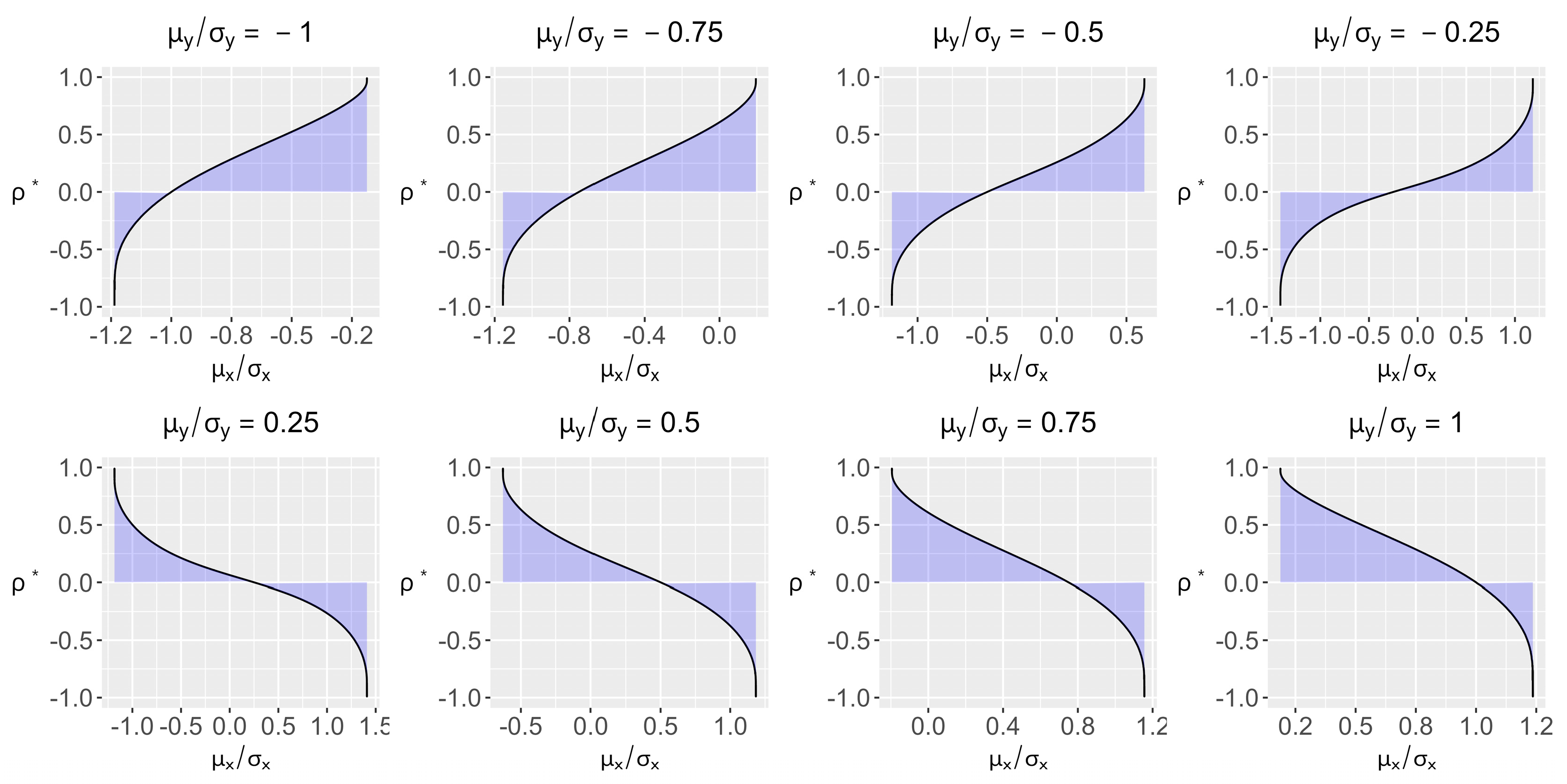
This relation implicitly defines a threshold function ${\rho }^{*}\left({\displaystyle \raisebox{1ex}{${\mu }_X$}\!\left/ \!\raisebox{-1ex}{${\sigma }_X$}\right.}\right)$ representing, for each ${\displaystyle \raisebox{1ex}{${\mu }_X$}\!\left/ \!\raisebox{-1ex}{${\sigma }_X$}\right.},$ the minimum correlation between X and Y required for the forecast X to match the directional accuracy of the uninformed benchmark Z:

• If ${\rho }_{YX}>{\rho }^{*}\left({\displaystyle \raisebox{1ex}{${\mu }_X$}\!\left/ \!\raisebox{-1ex}{${\sigma }_X$}\right.}\right), \mathrm{t}\mathrm{h}\mathrm{e}\mathrm{n} {\mathrm{M}\mathrm{D}\mathrm{A}}_X>{\mathrm{M}\mathrm{D}\mathrm{A}}_Z$;
• If ${\rho }_{YX}<{\rho }^{*}\left({\displaystyle \raisebox{1ex}{${\mu }_X$}\!\left/ \!\raisebox{-1ex}{${\sigma }_X$}\right.}\right), \mathrm{t}\mathrm{h}\mathrm{e}\mathrm{n} {\mathrm{M}\mathrm{D}\mathrm{A}}_X<{\mathrm{M}\mathrm{D}\mathrm{A}}_Z$.

Every time $0<{\rho }_{YX}<{\rho }^{*}\left({\displaystyle \raisebox{1ex}{${\mu }_X$}\!\left/ \!\raisebox{-1ex}{${\sigma }_X$}\right.}\right)$, we will have a case of strong MDA Paradox in which X is outperformed in terms of MDA by Z. (Strictly speaking, the function ${\rho }^{*}\left({\displaystyle \raisebox{1ex}{${\mu }_X$}\!\left/ \!\raisebox{-1ex}{${\sigma }_X$}\right.}\right)$ is defined only in the implicit domain where the left-hand side of (4) falls within the range attainable by the right-hand side, as $\rho$ varies in (−1, 1). Since ${\mathrm{\Phi }}_2\left(-{\displaystyle \frac{{\mu }_Y}{{\sigma }_Y}},-{\displaystyle \frac{{\mu }_X}{{\sigma }_X}};{\rho }_{YX}\right)$ is continuous and strictly increasing in ${\rho }_{YX}$, this requires that $2max\left\{0,\mathrm{\Phi }\left(-{\displaystyle \frac{{\mu }_Y}{{\sigma }_Y}}\right)+\mathrm{\Phi }\left(-{\displaystyle \frac{{\mu }_X}{{\sigma }_X}}\right)-1\right\}\le \mathrm{\Phi }\left(-{\displaystyle \frac{{\mu }_X}{{\sigma }_X}}\right)-\mathrm{\Phi }\left(-{\displaystyle \frac{{\mu }_Y}{{\sigma }_Y}}\right)+2{\mathrm{\Phi }}^2\left(-{\displaystyle \frac{{\mu }_Y}{{\sigma }_Y}}\right)\le 2min\left\{\mathrm{\Phi }\left(-{\displaystyle \frac{{\mu }_Y}{{\sigma }_Y}}\right),\mathrm{\Phi }\left(-{\displaystyle \frac{{\mu }_X}{{\sigma }_X}}\right)\right\}$. It is only under these conditions that a unique threshold ${\rho }^{*}\left({\displaystyle \raisebox{1ex}{${\mu }_X$}\!\left/ \!\raisebox{-1ex}{${\sigma }_X$}\right.}\right)$ exists in (−1, 1). Furthermore, it can be shown that ${\rho }^{*}\left({\displaystyle \raisebox{1ex}{${\mu }_X$}\!\left/ \!\raisebox{-1ex}{${\sigma }_X$}\right.}\right)$ is a monotonic function of ${\displaystyle \raisebox{1ex}{${\mu }_X$}\!\left/ \!\raisebox{-1ex}{${\sigma }_X$}\right.}$.

Figure 1 depicts these threshold functions for various levels of ${\displaystyle \raisebox{1ex}{${\mu }_Y$}\!\left/ \!\raisebox{-1ex}{${\sigma }_Y$}\right.}$. The shaded area in each figure represents Paradox zones. In particular, when ${\rho }_{YX}>0$, these are areas in which there is a positive correlation between forecast X and Y, yet this correlation is not large enough to match the MDA of the uninformative benchmark Z.

Notably, as shown by Figure 1, the threshold equals zero when ${\displaystyle \frac{{\mu }_X}{{\sigma }_X}}={\displaystyle \frac{{\mu }_Y}{{\sigma }_Y}}$, reflecting that a forecast with the same standardized mean as the target only needs to exhibit positive dependence with Y to improve upon an uninformative predictor Z that is also relatively unbiased (${\displaystyle \frac{{\mu }_Z}{{\sigma }_Z}}={\displaystyle \frac{{\mu }_Y}{{\sigma }_Y}}$).

Let us illustrate a case of strong MDA Paradox with a numerical example in which ${\displaystyle \frac{{\mu }_Y}{{\sigma }_Y}}={\displaystyle \frac{{\mu }_Z}{{\sigma }_Z}}=1$, ${\displaystyle \frac{{\mu }_X}{{\sigma }_X}} =0.25$ and ${\rho }_{YX}=0.25.$ According to Figure 1 (right inferior corner), forecast X will be outperformed by forecast Z in MDA despite having a larger correlation with the target variable. Let us compute the exact numbers:

$${\mathrm{M}\mathrm{D}\mathrm{A}}_Z=1-\mathrm{\Phi }\left(-1\right)-\mathrm{\Phi }\left(-1\right)+{2\mathrm{\Phi }}_2\left(-1,-1;0\right)=0.733$$

$${\mathrm{M}\mathrm{D}\mathrm{A}}_X=1-\mathrm{\Phi }\left(-1\right)-\mathrm{\Phi }\left(-0.25\right)+{2\mathrm{\Phi }}_2\left(-1,-0.25;0.25\right)=0.616$$

These numbers are consistent with Figure 1 and show a strong case of MDA Paradox, in which a totally independent forecast Z displays a higher MDA relative to a forecast X positively correlated with the target.

3.2.4. Two Extremely Biased Forecasts with Positive Correlation with the Target

Let us suppose now that both X and Z have a positive correlation with the target variable Y. Let us also assume that ${\displaystyle \frac{{\mu }_X}{{\sigma }_X}}\gg 0$ and ${\displaystyle \frac{{\mu }_Z}{{\sigma }_Z}}\ll 0$. In other words, the standardized mean of X is positive and very big, whereas the standardized mean of Z is negative and very big in absolute value. Then, the univariate terms in Expression (1) satisfies

$$\mathrm{\Phi }\left(-{\displaystyle \frac{{\mu }_X}{{\sigma }_X}}\right)\approx 0; \mathrm{\Phi }\left(-{\displaystyle \frac{{\mu }_Z}{{\sigma }_Z}}\right)\approx 1$$

So, the first term (P1) in ${\mathrm{M}\mathrm{D}\mathrm{A}}_X-{\mathrm{M}\mathrm{D}\mathrm{A}}_Z$ is close to 1. For the bivariate normal terms, we have

$${\mathrm{\Phi }}_2\left(-{\displaystyle \frac{{\mu }_Y}{{\sigma }_Y}},-{\displaystyle \frac{{\mu }_X}{{\sigma }_X}};{\rho }_{YX}\right)\approx 0; {\mathrm{\Phi }}_2\left(-{\displaystyle \frac{{\mu }_Y}{{\sigma }_Y}},-{\displaystyle \frac{{\mu }_Z}{{\sigma }_Z}};{\rho }_{YZ}\right)\approx \mathrm{\Phi }\left(-{\displaystyle \frac{{\mu }_Y}{{\sigma }_Y}}\right)$$

Therefore, the entire expression satisfies

$${\mathrm{M}\mathrm{D}\mathrm{A}}_X-{\mathrm{M}\mathrm{D}\mathrm{A}}_Z\approx 1-2\mathrm{\Phi }\left(-{\displaystyle \frac{{\mu }_Y}{{\sigma }_Y}}\right)=2\mathrm{\Phi }\left({\displaystyle \frac{{\mu }_Y}{{\sigma }_Y}}\right)-1$$

In this extreme case, the potential dependence of each forecast on the target variable plays no role in determining differences in MDA. The only subcomponents playing important roles are the standardized means ${\displaystyle \frac{{\mu }_X}{{\sigma }_X}},{\displaystyle \frac{{\mu }_Z}{{\sigma }_Z}}$ and ${\displaystyle \frac{{\mu }_Y}{{\sigma }_Y}}.$ On the one hand, when this latter ratio is positive:

$${\mathrm{M}\mathrm{D}\mathrm{A}}_X-{\mathrm{M}\mathrm{D}\mathrm{A}}_Z>0$$

indicating that X outperforms Z in correctly predicting the direction of Y. On the other hand, when ${\displaystyle \frac{{\mu }_Y}{{\sigma }_Y}}$ is negative,

$${\mathrm{M}\mathrm{D}\mathrm{A}}_X-{\mathrm{M}\mathrm{D}\mathrm{A}}_Z<0$$

indicating that Z outperforms X in correctly predicting the direction of Y. Notice that this is irrespective of the relative magnitudes of ${\rho }_{YX}$ and ${\rho }_{ZX}$. Here, paradoxical results emerge with clarity as the only relevant terms determining ${\mathrm{M}\mathrm{D}\mathrm{A}}_X-{\mathrm{M}\mathrm{D}\mathrm{A}}_Z$ are the standardized means of our forecasts and target variable.

Let us illustrate this scenario with a numerical example in which ${\displaystyle \frac{{\mu }_Y}{{\sigma }_Y}}=-0.25; {\displaystyle \frac{{\mu }_Z}{{\sigma }_Z}}=-2$, ${\displaystyle \frac{{\mu }_X}{{\sigma }_X}} =2$,${\rho }_{YZ}=0.25$ and ${\rho }_{YX}=0.75.$ Let us compute the exact numbers

$${\mathrm{M}\mathrm{D}\mathrm{A}}_Z=1-\mathrm{\Phi }\left(0.25\right)-\mathrm{\Phi }\left(2\right)+{2\mathrm{\Phi }}_2\left(\mathrm{0.25,2};0.25\right)=0.61$$

$${\mathrm{M}\mathrm{D}\mathrm{A}}_X=1-\mathrm{\Phi }\left(0.25\right)-\mathrm{\Phi }\left(-2\right)+{2\mathrm{\Phi }}_2\left(0.25,-2;0.75\right)=0.43$$

These numbers vividly show a strong case of MDA Paradox: although forecast Z has the weakest correlation with Y, it exhibits an MDA of 0.61, well above the 0.43 observed for X, the forecast with the highest correlation with the target variable.

3.2.5. A Constant Forecast vs. a Forecast with Positive Variance

Let X and Z be two forecasts for the same target variable Y with ${\mu }_Y\ne 0$. Let us further assume that Z is a constant c that is independent of Y, while X is positively correlated with the target variable (${\rho }_{YX}>0$)$.$ This implies that the correlation between forecast Z and Y is not defined. Nevertheless, Z and Y are independent with zero covariance. This example is inspired by a literature that frequently uses a constant forecast as a traditional benchmark to compare new forecasting alternatives, such as [25,26,27,28]. We already know that

$${\mathrm{M}\mathrm{D}\mathrm{A}}_X=1-\mathrm{\Phi }\left(-{\displaystyle \frac{{\mu }_Y}{{\sigma }_Y}}\right)-\mathrm{\Phi }\left(-{\displaystyle \frac{{\mu }_X}{{\sigma }_X}}\right)+{2\mathrm{\Phi }}_2\left(-{\displaystyle \frac{{\mu }_Y}{{\sigma }_Y}},-{\displaystyle \frac{{\mu }_X}{{\sigma }_X}};{\rho }_{YX}\right)$$

But we need to derive an expression for ${\mathrm{M}\mathrm{D}\mathrm{A}}_Z=\mathrm{Pr}\left(\mathrm{Y}\mathrm{Z}>0\right)=\mathrm{Pr}\left(cY>0\right)$. It follows that

$${\mathrm{M}\mathrm{D}\mathrm{A}}_Z=\mathrm{Pr}\left(\mathrm{Y}\mathrm{Z}>0\right)=\left\{\begin{array}{c}\mathrm{Pr}\left(Y>0\right) \mathrm{i}\mathrm{f} c>0\\ 0 \mathrm{i}\mathrm{f} c=0\\ \mathrm{Pr}\left(Y<0\right) \mathrm{i}\mathrm{f} c<0\end{array}\right.$$

This is equivalent to

$${\mathrm{M}\mathrm{D}\mathrm{A}}_Z=\mathrm{Pr}\left(\mathrm{Y}\mathrm{Z}>0\right)=\left\{\begin{array}{c}1-\mathrm{\Phi }\left(-{\displaystyle \frac{{\mu }_Y}{{\sigma }_Y}}\right)=\mathrm{\Phi }\left({\displaystyle \frac{{\mu }_Y}{{\sigma }_Y}}\right) \mathrm{i}\mathrm{f} c>0\\ 0 \mathrm{i}\mathrm{f} c=0\\ \mathrm{\Phi }\left(-{\displaystyle \frac{{\mu }_Y}{{\sigma }_Y}}\right) \mathrm{i}\mathrm{f} c<0\end{array}\right.$$

So, as long as $c\ne 0$, this constant forecast will have an MDA greater than 0.5 if the sign of c coincides with the sign of the expected value of Y. To explore potential paradoxical outcomes, we will assume both $c>0$ and ${\mu }_Y>0$. We have

$${\mathrm{M}\mathrm{D}\mathrm{A}}_X=1-\mathrm{\Phi }\left(-{\displaystyle \frac{{\mu }_Y}{{\sigma }_Y}}\right)-\mathrm{\Phi }\left(-{\displaystyle \frac{{\mu }_X}{{\sigma }_X}}\right)+{2\mathrm{\Phi }}_2\left(-{\displaystyle \frac{{\mu }_Y}{{\sigma }_Y}},-{\displaystyle \frac{{\mu }_X}{{\sigma }_X}};{\rho }_{YX}\right)$$

or

$${\mathrm{M}\mathrm{D}\mathrm{A}}_X=\mathrm{\Phi }\left({\displaystyle \frac{{\mu }_Y}{{\sigma }_Y}}\right)-\mathrm{\Phi }\left(-{\displaystyle \frac{{\mu }_X}{{\sigma }_X}}\right)+{2\mathrm{\Phi }}_2\left(-{\displaystyle \frac{{\mu }_Y}{{\sigma }_Y}},-{\displaystyle \frac{{\mu }_X}{{\sigma }_X}};{\rho }_{YX}\right)$$

Therefore

$${\mathrm{M}\mathrm{D}\mathrm{A}}_X-{\mathrm{M}\mathrm{D}\mathrm{A}}_Z=\mathrm{\Phi }\left({\displaystyle \frac{{\mu }_Y}{{\sigma }_Y}}\right)-\mathrm{\Phi }\left(-{\displaystyle \frac{{\mu }_X}{{\sigma }_X}}\right)+{2\mathrm{\Phi }}_2\left(-{\displaystyle \frac{{\mu }_Y}{{\sigma }_Y}},-{\displaystyle \frac{{\mu }_X}{{\sigma }_X}};{\rho }_{YX}\right)-\mathrm{\Phi }\left({\displaystyle \frac{{\mu }_Y}{{\sigma }_Y}}\right)$$

So, finally

$${\mathrm{M}\mathrm{D}\mathrm{A}}_X-{\mathrm{M}\mathrm{D}\mathrm{A}}_Z={2\mathrm{\Phi }}_2\left(-{\displaystyle \frac{{\mu }_Y}{{\sigma }_Y}},-{\displaystyle \frac{{\mu }_X}{{\sigma }_X}};{\rho }_{YX}\right)-\mathrm{\Phi }\left(-{\displaystyle \frac{{\mu }_X}{{\sigma }_X}}\right)$$

It turns out that if ${\displaystyle \frac{{\mu }_Y}{{\sigma }_Y}}⟶\infty$ while keeping ${\displaystyle \frac{{\mu }_X}{{\sigma }_X}}$ set at a fixed value, then ${2\mathrm{\Phi }}_2\left(-{\displaystyle \frac{{\mu }_Y}{{\sigma }_Y}},-{\displaystyle \frac{{\mu }_X}{{\sigma }_X}};{\rho }_{YX}\right)\approx 0$ and

$${\mathrm{M}\mathrm{D}\mathrm{A}}_X-{\mathrm{M}\mathrm{D}\mathrm{A}}_Z\approx -\mathrm{\Phi }\left(-{\displaystyle \frac{{\mu }_X}{{\sigma }_X}}\right)<0$$

Therefore, a constant forecast, which is entirely independent of the target variable Y, can nonetheless achieve higher MDA than a forecast X that is positively correlated with Y. Let us illustrate with a numerical example this situation. Let us suppose that: ${\mu }_Y={\mu }_X={\mu }_Z=0.5; {\displaystyle \frac{{\mu }_Y}{{\sigma }_Y}}=0.5$, ${\displaystyle \frac{{\mu }_X}{{\sigma }_X}} =0.125$ (so that ${\sigma }_X=4)$ and c = ${\mu }_Z=0.5$. We will also assume ${\rho }_{YX}=0.25.$ This implies

$$Cov(X,Y)>0=Cov(Y,Z).$$

In this case we have

$${\mathrm{M}\mathrm{D}\mathrm{A}}_X=1-\mathrm{\Phi }\left(-0.5\right)-\mathrm{\Phi }\left(-0.125\right)+{2\mathrm{\Phi }}_2\left(-0.5,-0.125;0.25\right)=0.59$$

$${\mathrm{M}\mathrm{D}\mathrm{A}}_Z=1-\mathrm{\Phi }\left(-0.5\right)=0.69$$

so that we clearly have a paradoxical case, in which $Cov\left(X,Y\right)>0=Cov\left(Y,Z\right),$ yet ${\mathrm{M}\mathrm{D}\mathrm{A}}_X=0.59 <{\mathrm{M}\mathrm{D}\mathrm{A}}_Z=0.69.$

3.2.6. An Independent Forecast vs. a Forecast with Positive Variance and Downward Bias

Let X and Z be two forecasts for the same target variable Y. Here we will assume that Z and Y are independent and that Z has a positive variance and zero mean: ${\mu }_Z=0.$ We will further assume that X is positively correlated with the target variable (${\rho }_{YX}>0$), and that ${\mu }_X<0; {\mu }_Y>0$ and the following condition holds true

$$\mathrm{\Phi }\left(-{\displaystyle \frac{{\mu }_X}{{\sigma }_X}}\right)-\mathrm{\Phi }\left(-{\displaystyle \frac{{\mu }_Y}{{\sigma }_Y}}\right)>0.5$$

These assumptions may seem arbitrary, yet they are similar to key features of our time series in the empirical illustration that we present in Section 5. Notice that our assumptions for Z and Y imply that Z coincides with a pure luck benchmark, that is, a forecast that delivers an MDA of 0.5. To see this, notice that

$$\begin{array}{ll}{\mathrm{M}\mathrm{D}\mathrm{A}}_Z=1-\mathrm{\Phi }& \left(-{\displaystyle \frac{{\mu }_Y}{{\sigma }_Y}}\right)-\mathrm{\Phi }\left(-{\displaystyle \frac{{\mu }_Z}{{\sigma }_Z}}\right)+{2\mathrm{\Phi }}_2\left(-{\displaystyle \frac{{\mu }_Y}{{\sigma }_Y}},-{\displaystyle \frac{{\mu }_Z}{{\sigma }_Z}};{\rho }_{YZ}\right)\\ & =1-\mathrm{\Phi }\left(-{\displaystyle \frac{{\mu }_Y}{{\sigma }_Y}}\right)-\mathrm{\Phi }\left(-{\displaystyle \frac{{\mu }_Z}{{\sigma }_Z}}\right)+2\mathrm{\Phi }\left(-{\displaystyle \frac{{\mu }_Y}{{\sigma }_Y}}\right)\mathrm{\Phi }\left(-{\displaystyle \frac{{\mu }_Z}{{\sigma }_Z}}\right)\\ & =1-\mathrm{\Phi }\left(-{\displaystyle \frac{{\mu }_Y}{{\sigma }_Y}}\right)-\mathrm{\Phi }\left(0\right)+2\mathrm{\Phi }\left(-{\displaystyle \frac{{\mu }_Y}{{\sigma }_Y}}\right)\mathrm{\Phi }\left(0\right)\\ & =0.5-\mathrm{\Phi }\left(-{\displaystyle \frac{{\mu }_Y}{{\sigma }_Y}}\right)+\mathrm{\Phi }\left(-{\displaystyle \frac{{\mu }_Y}{{\sigma }_Y}}\right)=0.5\end{array}$$

With this in mind, let us explore what Expression (1) tells us in these conditions

$$\begin{array}{ll}& {\mathrm{M}\mathrm{D}\mathrm{A}}_{\mathrm{X}}-{\mathrm{M}\mathrm{D}\mathrm{A}}_{\mathrm{Z}}=\mathrm{\Phi }\left(-{\displaystyle \frac{{\mathrm{\mu }}_{\mathrm{Z}}}{{\mathrm{\sigma }}_{\mathrm{Z}}}}\right)-\mathrm{\Phi }\left(-{\displaystyle \frac{{\mathrm{\mu }}_{\mathrm{X}}}{{\mathrm{\sigma }}_{\mathrm{X}}}}\right)+2\left[{\mathrm{\Phi }}_2\left(-{\displaystyle \frac{{\mathrm{\mu }}_{\mathrm{Y}}}{{\mathrm{\sigma }}_{\mathrm{Y}}}},-{\displaystyle \frac{{\mathrm{\mu }}_{\mathrm{X}}}{{\mathrm{\sigma }}_{\mathrm{X}}}};{\mathrm{\rho }}_{\mathrm{Y}\mathrm{X}}\right)-{\mathrm{\Phi }}_2\left(-{\displaystyle \frac{{\mathrm{\mu }}_{\mathrm{Y}}}{{\mathrm{\sigma }}_{\mathrm{Y}}}},-{\displaystyle \frac{{\mathrm{\mu }}_{\mathrm{Z}}}{{\mathrm{\sigma }}_{\mathrm{Z}}}};{\mathrm{\rho }}_{\mathrm{Y}\mathrm{Z}}\right)\right]\\ =& 0.5-\mathrm{\Phi }\left(-{\displaystyle \frac{{\mathrm{\mu }}_{\mathrm{X}}}{{\mathrm{\sigma }}_{\mathrm{X}}}}\right)+2\left[{\mathrm{\Phi }}_2\left(-{\displaystyle \frac{{\mathrm{\mu }}_{\mathrm{Y}}}{{\mathrm{\sigma }}_{\mathrm{Y}}}},-{\displaystyle \frac{{\mathrm{\mu }}_{\mathrm{X}}}{{\mathrm{\sigma }}_{\mathrm{X}}}};{\mathrm{\rho }}_{\mathrm{Y}\mathrm{X}}\right)-0.5\mathrm{\Phi }\left(-{\displaystyle \frac{{\mathrm{\mu }}_{\mathrm{Y}}}{{\mathrm{\sigma }}_{\mathrm{Y}}}}\right)\right]\\ =& 0.5-\left[\mathrm{\Phi }\left(-{\displaystyle \frac{{\mathrm{\mu }}_{\mathrm{X}}}{{\mathrm{\sigma }}_{\mathrm{X}}}}\right)+\mathrm{\Phi }\left(-{\displaystyle \frac{{\mathrm{\mu }}_{\mathrm{Y}}}{{\mathrm{\sigma }}_{\mathrm{Y}}}}\right)\right]+{2\mathrm{\Phi }}_2\left(-{\displaystyle \frac{{\mathrm{\mu }}_{\mathrm{Y}}}{{\mathrm{\sigma }}_{\mathrm{Y}}}},-{\displaystyle \frac{{\mathrm{\mu }}_{\mathrm{X}}}{{\mathrm{\sigma }}_{\mathrm{X}}}};{\mathrm{\rho }}_{\mathrm{Y}\mathrm{X}}\right)\end{array}$$

But, using that ${\mu }_X<0$ and ${\mu }_Y>0$, we have

$${\mathrm{\Phi }}_2\left(-{\displaystyle \frac{{\mu }_Y}{{\sigma }_Y}},-{\displaystyle \frac{{\mu }_X}{{\sigma }_X}};{\rho }_{YX}\right)\le min\left\{\mathrm{\Phi }\left(-{\displaystyle \frac{{\mu }_X}{{\sigma }_X}}\right),\mathrm{\Phi }\left(-{\displaystyle \frac{{\mu }_Y}{{\sigma }_Y}}\right)\right\}=\mathrm{\Phi }\left(-{\displaystyle \frac{{\mu }_Y}{{\sigma }_Y}}\right)$$

Therefore

$${\mathrm{M}\mathrm{D}\mathrm{A}}_X-{\mathrm{M}\mathrm{D}\mathrm{A}}_Z\le 0.5-\left[\mathrm{\Phi }\left(-{\displaystyle \frac{{\mu }_X}{{\sigma }_X}}\right)+\mathrm{\Phi }\left(-{\displaystyle \frac{{\mu }_Y}{{\sigma }_Y}}\right)\right]+2\mathrm{\Phi }\left(-{\displaystyle \frac{{\mu }_Y}{{\sigma }_Y}}\right)$$

So

$${\mathrm{M}\mathrm{D}\mathrm{A}}_X-{\mathrm{M}\mathrm{D}\mathrm{A}}_Z\le 0.5+\mathrm{\Phi }\left(-{\displaystyle \frac{{\mu }_Y}{{\sigma }_Y}}\right)-\mathrm{\Phi }\left(-{\displaystyle \frac{{\mu }_X}{{\sigma }_X}}\right)<0$$

Therefore, forecast Z, which is entirely independent of the target variable Y, can nonetheless achieve higher MDA than a forecast X that is positively correlated with Y. Let us illustrate this case with a numerical example. Let us suppose that: ${\displaystyle \frac{{\mu }_Y}{{\sigma }_Y}}=0.5$, ${\displaystyle \frac{{\mu }_X}{{\sigma }_X}} =-1$ and ${\rho }_{YX}=0.5.$ This implies

$$\mathrm{\Phi }\left(-{\displaystyle \frac{{\mu }_Y}{{\sigma }_Y}}\right)=0.31, \mathrm{\Phi }\left(-{\displaystyle \frac{{\mu }_X}{{\sigma }_X}}\right)=0.84$$

and

$${\mathrm{M}\mathrm{D}\mathrm{A}}_X=1-\mathrm{\Phi }\left(-0.5\right)-\mathrm{\Phi }\left(1\right)+{2\mathrm{\Phi }}_2\left(-0.5,1;0.5\right)=0.44$$

$${\mathrm{M}\mathrm{D}\mathrm{A}}_Z=0.5$$

So we clearly have a paradoxical case, in which ${\rho }_{YX}>0={\rho }_{YZ},$ yet ${\mathrm{M}\mathrm{D}\mathrm{A}}_X=0.44 <{\mathrm{M}\mathrm{D}\mathrm{A}}_Z=0.5.$ We will return to this case in Section 5, where we discuss the paradoxical results observed in our empirical application.

4. Conditions Under Which the MDA Paradox Is Impossible

In this section we focus on establishing two results that provide different sets of conditions under which the MDA Paradox is impossible. We also show a very interesting proposition that allows for a simple computation of MDA differentials when forecasts are unbiased and the target variable has zero mean. Before presenting all these results, we show and prove the following Lemma 2, which is very simple, but we use it later in Proposition 2.

Lemma 2.

Let ${\mathrm{\Phi }}_2\left(a,b;\rho \right)$ denote the cumulative distribution function of the standard bivariate normal distribution with correlation coefficient $\rho \in (-1, 1)$, evaluated at the fixed point $(a,b)$ $\in {\mathbb{R}}^2.$ Then

$${\displaystyle \frac{\partial {\mathrm{\Phi }}_2\left(a,b;\rho \right)}{\partial b}}=\mathrm{\varphi }\left(b\right)\mathrm{\Phi }\left({\displaystyle \frac{a-\rho b}{\sqrt{1-{\rho }^2}}}\right)$$

Proof of Lemma 2.

Let (X,Y) be a random vector that follows a standard bivariate normal distribution with correlation coefficient $\rho \in \left(-1, 1\right)$. It follows that

$$X|Y\rightsquigarrow N(\rho y,1-{\rho }^2)$$

Then

$$\mathrm{P}\mathrm{r}\left(X\le a|Y=y\right)=\mathrm{P}\mathrm{r}\left({\displaystyle \frac{X-\rho y}{\sqrt{1-{\rho }^2}}}\le {\displaystyle \frac{a-\rho y}{\sqrt{1-{\rho }^2}}}|Y=y\right)=\mathrm{\Phi }\left({\displaystyle \frac{a-\rho y}{\sqrt{1-{\rho }^2}}}\right)$$

Therefore

$${\mathrm{\Phi }}_2\left(a,b;\rho \right)=\mathrm{P}\mathrm{r}\left(X\le a,Y\le b\right)={\int }_{-\infty }^b\mathrm{P}\mathrm{r}\left(X\le a|Y=y\right)f_Y\left(y\right)dy={\int }_{-\infty }^b\mathrm{\Phi }\left({\displaystyle \frac{a-\rho y}{\sqrt{1-{\rho }^2}}}\right)f_Y\left(y\right)dy$$

and

$${\displaystyle \frac{\partial {\mathrm{\Phi }}_2\left(a,b;\rho \right)}{\partial b}}=\mathrm{\varphi }\left(b\right)\mathrm{\Phi }\left({\displaystyle \frac{a-\rho b}{\sqrt{1-{\rho }^2}}}\right),$$

which is the desired result. □

The following proposition establishes that, under Mincer–Zarnowitz efficiency, paradoxical results with respect to MDA and correlations cannot arise. This result is in line with the MSPE Paradox, which is likewise impossible when forecasts are efficient (see [6,8]).

Proposition 2.

In the context of Proposition 1, if both forecasts X and Z are Mincer–Zarnowitz [10] efficient, that is to say

$${\mu }_X={\mu }_Z={\mu }_Y=\mu , \hspace{1em}{\rho }_{YX}={\displaystyle \frac{{\sigma }_X}{{\sigma }_Y}} \ge 0, \hspace{1em}{\rho }_{YZ}={\displaystyle \frac{{\sigma }_Z}{{\sigma }_Y}} \ge 0; {\rho }_{YX}<1 \mathrm{a}\mathrm{n}\mathrm{d} {\rho }_{YZ}<1$$

Then the MDA Paradox is impossible.

Proof of Proposition 2.

We begin by expressing the MDA associated with forecast X

$${\mathrm{M}\mathrm{D}\mathrm{A}}_X=1-\mathrm{\Phi }\left(-{\displaystyle \frac{\mu }{{\sigma }_Y}}\right)-\mathrm{\Phi }\left(-{\displaystyle \frac{\mu }{{\sigma }_X}}\right)+{2\mathrm{\Phi }}_2\left(-{\displaystyle \frac{\mu }{{\sigma }_Y}},-{\displaystyle \frac{\mu }{{\sigma }_X}};{\displaystyle \frac{{\sigma }_X}{{\sigma }_Y}}\right)$$

Define the function

$${g\left({\sigma }_X\right)\equiv 2\mathrm{\Phi }}_2\left(-{\displaystyle \frac{\mu }{{\sigma }_Y}},-{\displaystyle \frac{\mu }{{\sigma }_X}};{\displaystyle \frac{{\sigma }_X}{{\sigma }_Y}}\right)-\mathrm{\Phi }\left(-{\displaystyle \frac{\mu }{{\sigma }_X}}\right),$$

then

$${\mathrm{M}\mathrm{D}\mathrm{A}}_X=1-\mathrm{\Phi }\left(-{\displaystyle \frac{\mu }{{\sigma }_Y}}\right)+g({\sigma }_X)$$

By symmetry, the MDA associated with forecast Z can be written as

$${\mathrm{M}\mathrm{D}\mathrm{A}}_Z=1-\mathrm{\Phi }\left(-{\displaystyle \frac{\mu }{{\sigma }_Y}}\right)+g({\sigma }_Z)$$

Hence,

$${\mathrm{M}\mathrm{D}\mathrm{A}}_X-{\mathrm{M}\mathrm{D}\mathrm{A}}_Z=g\left({\sigma }_X\right)-g\left({\sigma }_Z\right)$$

Let us continue analyzing the function $g\left({\sigma }_X\right)$ keeping in mind that the case of $g\left({\sigma }_Z\right)$ follows by symmetry. Given ${\sigma }_Y>0$ and $\mu \in \mathbb{R},$ $g\left({\sigma }_X\right)$ is an increasing function of ${\sigma }_X$. To see this, we will compute its derivative

$${\displaystyle \frac{\partial \mathrm{g}\left({\sigma }_X\right)}{\partial {\sigma }_X}}=g^{\prime }\left({\sigma }_X\right)={\displaystyle \frac{{2\partial \mathrm{\Phi }}_2\left(-\frac{\mu }{{\sigma }_Y},-\frac{\mu }{{\sigma }_X};\frac{{\sigma }_X}{{\sigma }_Y}\right)}{\partial {\sigma }_X}}-{\displaystyle \frac{\partial \mathrm{\Phi }\left(-\frac{\mu }{{\sigma }_X}\right)}{\partial {\sigma }_X}}$$

The derivative of the univariate Gaussian distribution in the right-hand side is straightforward:

$${\displaystyle \frac{\partial \mathrm{\Phi }\left(-\frac{\mu }{{\sigma }_X}\right)}{\partial {\sigma }_X}}=\mathrm{\varphi }\left(-{\displaystyle \frac{\mu }{{\sigma }_X}}\right){\displaystyle \frac{\mu }{{\sigma }_X^2}}$$

For the derivative of the bivariate Gaussian distribution, we have

$${\displaystyle \frac{{2\partial \mathrm{\Phi }}_2\left(-\frac{\mu }{{\sigma }_Y},-\frac{\mu }{{\sigma }_X};\frac{{\sigma }_X}{{\sigma }_Y}\right)}{\partial {\sigma }_X}}=2\left[{\displaystyle \frac{\partial {\mathrm{\Phi }}_2}{\partial b}}{\displaystyle \frac{\partial b}{\partial {\sigma }_X}}+{\displaystyle \frac{\partial {\mathrm{\Phi }}_2}{\partial \rho }}{\displaystyle \frac{\partial \rho }{\partial {\sigma }_X}}\right]$$

where $a=-{\displaystyle \frac{\mu }{{\sigma }_Y}}$; $b=-{\displaystyle \frac{\mu }{{\sigma }_X}}$, and $\rho ={\displaystyle \frac{{\sigma }_X}{{\sigma }_Y}}$.

From Lemmas 1 and 2 we obtain

$${\displaystyle \frac{\partial {\mathrm{\Phi }}_2\left(a,b;\rho \right)}{\partial \rho }}={\mathrm{\varphi }}_2\left(a,b;\rho \right)$$

$${\displaystyle \frac{\partial {\mathrm{\Phi }}_2\left(a,b;\rho \right)}{\partial b}}=\mathrm{\varphi }\left(b\right)\mathrm{\Phi }\left({\displaystyle \frac{a-\rho b}{\sqrt{1-{\rho }^2}}}\right)$$

Furthermore

$${\displaystyle \frac{\partial b}{\partial {\sigma }_X}}={\displaystyle \frac{\mu }{{\sigma }_X^2}}=-{\displaystyle \frac{b}{{\sigma }_X}}, \hspace{1em}{\displaystyle \frac{\partial \rho }{\partial {\sigma }_X}}={\displaystyle \frac{1}{{\sigma }_Y}}$$

Therefore, we have

$$g^{\prime }\left({\sigma }_X\right)=2\left[\mathrm{\varphi }\left(b\right)\mathrm{\Phi }\left({\displaystyle \frac{a-\rho b}{\sqrt{1-{\rho }^2}}}\right){\displaystyle \frac{\mu }{{\sigma }_X^2}}+{\mathrm{\varphi }}_2\left(a,b;\rho \right){\displaystyle \frac{1}{{\sigma }_Y}}\right]-\mathrm{\varphi }\left(-{\displaystyle \frac{\mu }{{\sigma }_X}}\right){\displaystyle \frac{\mu }{{\sigma }_X^2}},$$

or simply

$$g^{\prime }\left({\sigma }_X\right)=2\left[-\mathrm{\varphi }\left(b\right)\mathrm{\Phi }\left({\displaystyle \frac{a-\rho b}{\sqrt{1-{\rho }^2}}}\right){\displaystyle \frac{b}{{\sigma }_X}}+{\mathrm{\varphi }}_2\left(a,b;\rho \right){\displaystyle \frac{1}{{\sigma }_Y}}\right]+\mathrm{\varphi }\left(b\right){\displaystyle \frac{b}{{\sigma }_X}}$$

Rearranging terms we have

$$g^{\prime }\left({\sigma }_X\right)=\mathrm{\varphi }\left(b\right){\displaystyle \frac{b}{{\sigma }_X}}\left[1-2\mathrm{\Phi }\left({\displaystyle \frac{a-\rho b}{\sqrt{1-{\rho }^2}}}\right)\right]+2{\varphi }_2\left(a,b;\rho \right){\displaystyle \frac{1}{{\sigma }_Y}},$$

but

$$a-\rho b=-{\displaystyle \frac{\mu }{{\sigma }_Y}}-{\displaystyle \frac{{\sigma }_X}{{\sigma }_Y}}\left[-{\displaystyle \frac{\mu }{{\sigma }_X}}\right]=-{\displaystyle \frac{\mu }{{\sigma }_Y}}+{\displaystyle \frac{\mu }{{\sigma }_Y}}=0$$

Therefore

$$\mathrm{\Phi }\left({\displaystyle \frac{a-\rho b}{\sqrt{1-{\rho }^2}}}\right)=\mathrm{\Phi }\left(0\right)=0.5,$$

which means that

$$g^{\prime }\left({\sigma }_X\right)=2{\varphi }_2\left(a,b;\rho \right){\displaystyle \frac{1}{{\sigma }_Y}}>0$$

Thus, $g\left({\sigma }_X\right)$ is an increasing function in ${\sigma }_X.$ Consequently, whenever

$${\rho }_{YX}={\displaystyle \frac{{\sigma }_X}{{\sigma }_Y}}>{\rho }_{YZ}={\displaystyle \frac{{\sigma }_Z}{{\sigma }_Y}}$$

we will have ${\sigma }_X> {\sigma }_Z$, which leads to

$${\mathrm{M}\mathrm{D}\mathrm{A}}_X-{\mathrm{M}\mathrm{D}\mathrm{A}}_Z=g\left({\sigma }_X\right)-g\left({\sigma }_Z\right)\ge 0$$

Hence, the MDA-Correlation Paradox cannot arise when both forecasts are Mincer–Zarnowitz [10] efficient, which completes the proof. □

Proposition 2 indicates that the MDA Paradox cannot occur when comparing Mincer–Zarnowitz [10] efficient forecasts. This is an important result. However, since violations of efficiency are fairly common in the forecasting literature, it is important to explore some conditions under which the MDA Paradox may still be prevented in the presence of inefficient forecasts. (Violations of forecast efficiency have been documented across a wide range of variables in numerous studies. See [29,30,31,32,33] among others.) This is precisely addressed in the following Lemma 3.

Lemma 3.

In the context of Proposition 1, and assuming ${\rho }_{YX}, {\rho }_{YZ}\mathrm{ϵ}\left(-1, 1\right),$ if the standardized means of both forecasts are the same

$${\displaystyle \frac{{\mu }_Z}{{\sigma }_Z}}={\displaystyle \frac{{\mu }_X}{{\sigma }_X}}=\theta ,$$

(5)

then paradoxical results between MDA and correlations are impossible.

Proof of Lemma 3:

Using (5) in (1) we get

$${\mathrm{M}\mathrm{D}\mathrm{A}}_X-{\mathrm{M}\mathrm{D}\mathrm{A}}_Z=\mathrm{\Phi }\left(-\theta \right)-\mathrm{\Phi }\left(-\theta \right)+2\left[{\mathrm{\Phi }}_2\left(-{\displaystyle \frac{{\mu }_Y}{{\sigma }_Y}},-\theta ;{\rho }_{YX}\right)-{\mathrm{\Phi }}_2\left(-{\displaystyle \frac{{\mu }_Y}{{\sigma }_Y}},-\theta ;{\rho }_{YZ}\right)\right],$$

so

$${\mathrm{M}\mathrm{D}\mathrm{A}}_X-{\mathrm{M}\mathrm{D}\mathrm{A}}_Z=2\left[{\mathrm{\Phi }}_2\left(-{\displaystyle \frac{{\mu }_Y}{{\sigma }_Y}},-\theta ;{\rho }_{YX}\right)-{\mathrm{\Phi }}_2\left(-{\displaystyle \frac{{\mu }_Y}{{\sigma }_Y}},-\theta ;{\rho }_{YZ}\right)\right]$$

If ${\rho }_{YX}>{\rho }_{YZ}$, Lemma 1 implies that the right-hand side in the previous expression is non-negative, which in turn means that

$${\mathrm{M}\mathrm{D}\mathrm{A}}_X-{\mathrm{M}\mathrm{D}\mathrm{A}}_Z\ge 0$$

and no paradoxical results between correlations and MDA can emerge as stated. □

Lemma 3 and Proposition 2 establish clear sufficient conditions under which the MDA Paradox is impossible. It remains to investigate whether a simpler condition, such as unbiasedness, is also sufficient to prevent this paradox. Although the simple example in Section 3.2.5 shows that this is not the case, it turns out that unbiased forecasts, in the context of a mean-zero target variable, fall within the framework of Lemma 3. (In the numerical illustration in example Section 3.2.5, we already showed that the MDA Paradox emerges when both forecasts are unbiased. In this particular example we assumed ${\mu }_Y={\mu }_X={\mu }_Z=0.5$.) Interestingly, in this setting, a closed-form expression for the difference in MDA is also available, as we shall see next.

Proposition 3.

In the context of Proposition 1, if ${\rho }_{YX}, {\rho }_{YZ} ϵ \left(-1, 1\right)$ and both forecasts X and Z are unbiased for the mean-zero target variable Y, that is to say

$${\mu }_X={\mu }_Z={\mu }_Y=0$$

Then

$${\mathrm{M}\mathrm{D}\mathrm{A}}_{\mathrm{X}}-{\mathrm{M}\mathrm{D}\mathrm{A}}_{\mathrm{Z}}={\displaystyle \frac{1}{\pi }}\left[\arcsin \left({\rho }_{YX}\right)-\arcsin \left({\rho }_{YZ}\right) \right],$$

and the MDA Paradox is impossible.

Proof of Proposition 3.

If X and Y are jointly normal random variables with mean zero, unit variances and correlation coefficient $\rho \in \left(-1, 1\right),$ then we have

$$\mathrm{P}\mathrm{r}\left(X>0,Y>0\right)={\int }_0^{\infty }{\int }_0^{\infty }{\displaystyle \frac{1}{2\pi }}{\displaystyle \frac{1}{\sqrt{1-{\rho }^2}}}{e}^{-{\displaystyle \frac{1}{2}}{\displaystyle \frac{\left(x^2-2xy\rho +y^2\right)}{1-{\rho }^2}}}dxdy$$

Using polar coordinates $x=r\cos \theta , y=r\sin \theta$, we can write this probability as

$${\displaystyle \frac{1}{2\pi }}{\displaystyle \frac{1}{\sqrt{1-{\rho }^2}}}{\int }_0^{{\displaystyle \frac{\pi }{2}}}{\int }_0^{\infty }{e}^{-{\displaystyle \frac{1}{2}}{\displaystyle \frac{\left(1-\rho \sin 2\theta \right)}{1-{\rho }^2}}{r}^2}rdrd\theta$$

Let $A\left(\theta \right)={\displaystyle \frac{1-\rho \sin 2\theta }{1-{\rho }^2}}$, then using the following change in variables

$$u={\displaystyle \frac{1}{2}}A\left(\theta \right)r^2⟹du=A\left(\theta \right)rdr, r=0⟹u=0, r⟶\infty ⟹u⟶\infty ;$$

we get

$${\int }_0^{\infty }{e}^{-{\displaystyle \frac{1}{2}}{\displaystyle \frac{\left(1-\rho \sin 2\theta \right)}{1-{\rho }^2}}{r}^2}rdr={\int }_0^{\infty }{e}^{-{\displaystyle \frac{1}{2}}A\left(\theta \right)r^2}rdr={\displaystyle \frac{1}{A\left(\theta \right)}}{\int }_0^{\infty }{e}^{-u}du={\displaystyle \frac{1}{A\left(\theta \right)}}$$

Thus

$$\mathrm{P}\mathrm{r}\left(X>0,Y>0\right)={\displaystyle \frac{1}{2\pi }}{\displaystyle \frac{1}{\sqrt{1-{\rho }^2}}}{\int }_0^{{\displaystyle \frac{\pi }{2}}}{\displaystyle \frac{1-{\rho }^2}{1-\rho \sin 2\theta }}d\theta ={\displaystyle \frac{\sqrt{1-{\rho }^2}}{2\pi }}{\int }_0^{{\displaystyle \frac{\pi }{2}}}{\displaystyle \frac{1}{1-\rho \sin 2\theta }}d\theta$$

Let $v=\tan \theta ⟹\mathrm{d}v={\sec }^2\theta d\theta =\left({\tan }^2\theta +1\right)d\theta =\left(v^2+1\right)d\theta$.

Moreover, $\sin 2\theta =2\sin \theta \cos \theta =2{\displaystyle \frac{\tan \theta }{{\tan }^2\theta +1}}={\displaystyle \frac{2v}{v^2+1}}$. Thus, the probability $\mathrm{P}\mathrm{r}\left(X>0,Y>0\right)$ equals

$$\begin{array}{ll}& \mathrm{P}\mathrm{r}\left(X>0,Y>0\right)={\displaystyle \frac{\sqrt{1-{\rho }^2}}{2\pi }}{\int }_0^{\infty }\left[{\displaystyle \frac{1}{1-\rho \left(\frac{2v}{v^2+1}\right)}}\right]{\displaystyle \frac{dv}{v^2+1}}={\displaystyle \frac{\sqrt{1-{\rho }^2}}{2\pi }}{\int }_0^{\infty }{\displaystyle \frac{dv}{v^2+1-2v\rho }}\\ ={\displaystyle \frac{\sqrt{1-{\rho }^2}}{2\pi }}& {\int }_0^{\infty }{\displaystyle \frac{1}{{\left(v-\rho \right)}^2+1-{\rho }^2}}dv={\displaystyle \frac{\sqrt{1-{\rho }^2}}{2\pi }}{\int }_{-\rho }^{\infty }{\displaystyle \frac{1}{u^2+{\sqrt{1-{\rho }^2}}^2}}du\\ ={\displaystyle \frac{\sqrt{1-{\rho }^2}}{2\pi }}& {\displaystyle \frac{1}{\sqrt{1-{\rho }^2}}}\arctan {\left.\left({\displaystyle \frac{u}{\sqrt{1-{\rho }^2}}}\right)\right|}_{-\rho }^{\infty }={\displaystyle \frac{1}{2\pi }}\left[{\displaystyle \frac{\pi }{2}}-\arctan \left({\displaystyle \frac{-\rho }{\sqrt{1-{\rho }^2}}}\right)\right]\\ ={\displaystyle \frac{1}{4}}-{\displaystyle \frac{1}{2\pi }}& \arctan \left({\displaystyle \frac{-\rho }{\sqrt{1-{\rho }^2}}}\right)={\displaystyle \frac{1}{4}}+{\displaystyle \frac{1}{2\pi }}\arctan \left({\displaystyle \frac{\rho }{\sqrt{1-{\rho }^2}}}\right)\end{array}$$

In this last step we have used that arctan is an odd function. Let us express $\rho =\sin \left(\phi \right)$ for $\phi \in \left(-{\displaystyle \frac{\pi }{2}};{\displaystyle \frac{\pi }{2}}\right).$ Given that ${\mathrm{s}\mathrm{i}\mathrm{n}}^2\left(\phi \right)$+${\mathrm{c}\mathrm{o}\mathrm{s}}^2\left(\phi \right)$=1, we get ${\mathrm{c}\mathrm{o}\mathrm{s}}^2\left(\phi \right)=1-{\rho }^2$ which means $\cos \left(\phi \right)=\sqrt{1-{\rho }^2.}$ Therefore $\tan \left(\phi \right)={\displaystyle \frac{\rho }{\sqrt{1-{\rho }^2}}}$ which means $\phi =\mathrm{a}\mathrm{r}\mathrm{c}\mathrm{t}\mathrm{a}\mathrm{n}\left({\displaystyle \frac{\rho }{\sqrt{1-{\rho }^2}}}\right)$. Yet, we started with $\rho =\sin \left(\phi \right)$ which in turn means, $\phi =\mathrm{a}\mathrm{r}\mathrm{c}\mathrm{s}\mathrm{i}\mathrm{n}\left(\rho \right)$. This leads to the equality $\mathrm{a}\mathrm{r}\mathrm{c}\mathrm{t}\mathrm{a}\mathrm{n}\left({\displaystyle \frac{\rho }{\sqrt{1-{\rho }^2}}}\right)=\mathrm{a}\mathrm{r}\mathrm{c}\mathrm{s}\mathrm{i}\mathrm{n}(\rho )$. So we finally have

$$\mathrm{P}\mathrm{r}\left(X>0,Y>0\right)={\displaystyle \frac{1}{4}}+{\displaystyle \frac{1}{2\pi }}\mathrm{a}\mathrm{r}\mathrm{c}\mathrm{s}\mathrm{i}\mathrm{n}\left(\rho \right)$$

which is an increasing function of $\rho$ as given by the derivative

$${\displaystyle \frac{d\left(\mathrm{a}\mathrm{r}\mathrm{c}\mathrm{s}\mathrm{i}\mathrm{n}\left(\rho \right)\right)}{d\rho }}={\displaystyle \frac{1}{\sqrt{1-{\rho }^2}}}>0;\left|\rho \right|<1$$

Recalling that

$${\mathrm{M}\mathrm{D}\mathrm{A}}_{\mathrm{X}}=\mathrm{P}\mathrm{r}\left(\mathrm{Y}\mathrm{X}>0\right)=\mathrm{P}\mathrm{r}\left(\mathrm{Y}>0,\mathrm{X}>0\right)+\mathrm{P}\mathrm{r}\left(\mathrm{Y}\le 0,\mathrm{X}\le 0\right),$$

and using the symmetry of the bivariate normal distribution with zero means and equal variances, we get

$${\mathrm{M}\mathrm{D}\mathrm{A}}_X=2\mathrm{P}\mathrm{r}\left(Y>0,X>0\right)={\displaystyle \frac{1}{2}}+{\displaystyle \frac{1}{\pi }}\arcsin \left(\rho \right),$$

which finally leads to

$${\mathrm{M}\mathrm{D}\mathrm{A}}_X-{\mathrm{M}\mathrm{D}\mathrm{A}}_Z={\displaystyle \frac{1}{\pi }}\left[\arcsin \left({\rho }_{YX}\right)-\arcsin \left({\rho }_{YZ}\right) \right]$$

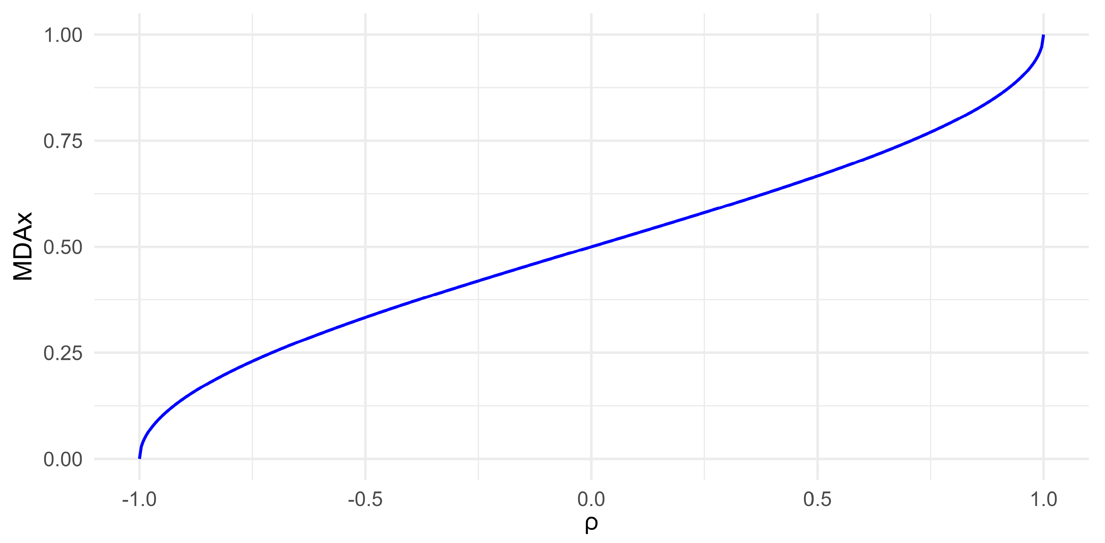
which is the desired result. Figure 2 represents ${\mathrm{M}\mathrm{D}\mathrm{A}}_X$ as a function of $\rho$. □

5. Empirical Illustration

In this section, we illustrate the MDA Paradox with an application in the context of the exchange rate forecasting literature. Our target variable is the Chilean Peso (CLP) vis-à-vis the US Dollar. We evaluate forecasts from the Survey of Professional Forecasters (SPF) conducted by the Central Bank of Chile. Specifically, we use monthly observations of the Chilean Peso and SPF forecasts for the period April 2012–April 2024. For exchange rate data, we extract the daily closing price of the CLP from Bloomberg and convert them to monthly frequencies by sampling from the last day of each month. We also sample the closing price from the day before the survey is released. The latter time series is simply denoted as CLP+. We will explain in brief why we consider two different time series for the Chilean Peso. Data from the SPF are directly obtained from the Central Bank of Chile. During the sample period, the survey release date varied between the 9th and 13th of each month.

We will use the following notation: ${\mathrm{S}}_{\mathrm{t}}$ denotes the Chilean Peso at month t. Being more specific, ${\mathrm{S}}_{\mathrm{t}}$ represents the amount of Chilean Pesos required to buy one U.S. Dollar at the closing price of the last day of month t. So, and just to give an example, if month t corresponds to January, ${\mathrm{S}}_{\mathrm{t}}$ corresponds to the closing price of the CLP in January 31st. If follows in this example, that ${\mathrm{S}}_{\mathrm{t}+1}$ would represent the closing price of the CLP in February 28. We have already mentioned that the survey is released to the public sometime in the middle of each month. We will use the notation ${\mathrm{S}}_{\mathrm{t}+}$ to generically denote the closing price of the CLP the day before the survey is released. So, following with the previous example, if the survey is released in February the 10th, then ${\mathrm{S}}_{\mathrm{t}+}$ would represent the closing price of the CLP in February the 9th. So, the following inequality describes the timeline in the flow of information: $t<t+<t+1$.

We have spent a few lines describing this timeline because we want to assess the predictive ability of the survey, which is released around the middle of each month. So, following with the previous example, if the survey is released in February 10th the difference ${\mathrm{S}}_{\mathrm{t}+1}-{\mathrm{S}}_{\mathrm{t}}$ is not entirely unknown. This variation represents how the CLP changes from the end of January to the end of February. Yet, at the moment the survey is released we already know what happened in the first nine days of February. More generally

$${\mathrm{S}}_{\mathrm{t}+1}-{\mathrm{S}}_{\mathrm{t}}=\left[{\mathrm{S}}_{\mathrm{t}+1}-{\mathrm{S}}_{\mathrm{t}+}\right]+\left[{\mathrm{S}}_{\mathrm{t}+}-{\mathrm{S}}_{\mathrm{t}}\right]$$

The only unknown variable in the right-hand side of the previous expression is $\left[{\mathrm{S}}_{\mathrm{t}+1}-{\mathrm{S}}_{\mathrm{t}+}\right]$, so that would be the focus of our interest. The survey asks for forecasts at three different horizons: 2, 11 and 23 months ahead. The Central Bank of Chile provides the median values across all respondents. We label SPF2, SPF11 and SPF23 the time-series containing the median of these forecasts 2, 11 and 23 months ahead, respectively. An important observation is in order: we consider each time-series SPF2, SPF11 and SPF23 as independent forecasts for the Chilean exchange rate and we explore their ability to correctly predict the Chilean Peso at different forecasting horizons h, varying from h = 1, 2, 3, 6, 9, 11, 12, 18 and 24 months ahead. So, despite SPF2 being the median of the respondents regarding the question for the Chilean exchange rate 2 months ahead, we explore also if this answer is useful to predict at the shortest horizon of one month, as well as the longer horizons of 3, 6, 9, 11, 12, 18 and 24 months ahead. This is in line with previous work by [28] who showed that SPF2, SPF11 and SPF23 could be useful forecasts of the Chilean Peso at several horizons.

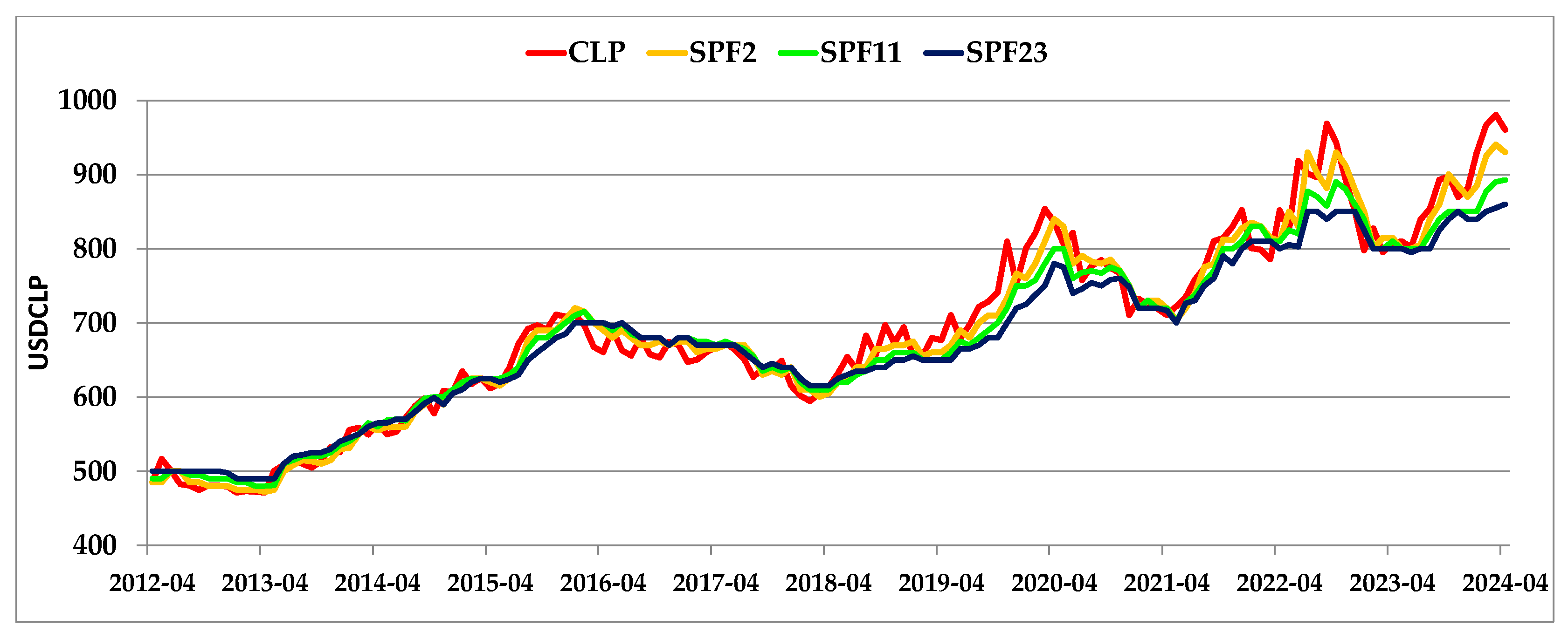
Figure 3 depicts the Chilean peso (our target variable) during the sample period of interest and the time series of our three forecasts SPF2, SPF11 and SPF23. This figure reveals an upward trend in all four series, which is a clear evidence of a non-stationary behavior. To avoid any potential spurious results that are so frequent in the analysis of trending data or, more generally, non-stationary data, we focus on forecasting Chilean Peso log-returns, rather than the Chilean Peso itself.

Figure 3 shows that all three forecasts, SPF2, SPF11 and SPF23, closely tracked the Chilean Peso during the early part of our sample period, from April 2012 to May 2018. After that, however, the three forecasts display a systematic downward bias, consistently underestimating the value of the US Dollar. Furthermore, in the latter half of the sample, SPF2 tends to lie above SPF11, which in turn tends to lie above SPF23. This ordering suggests that the median forecaster expected the Chilean Peso to strengthen as the forecasting horizon increased, an outcome that did not materialize during this period. Our predictive analysis focuses on the second part of the sample period, from June 2018 to April 2024. We do so partly because Ref. [28] analyzes the same data set only up to May 2018, and partly because of the previously documented downward bias in the survey. As will become evident below, this biased behavior appears to be a key element underlying the paradoxical results that follow.

We use lower-case letters to denote the natural logarithm of a variable, so that: ${\mathrm{s}}_{\mathrm{t}}\equiv \ln \left({\mathrm{S}}_{\mathrm{t}}\right).$ The h-period log-return of the Chilean Peso is defined as

$${\mathrm{r}}_{t^{+},t+h}=s_{t+h}-s_{t^{+}}$$

We focus on forecasts of this variable at horizons of h = 1, 2, 3, 6, 9, 11, 12, 18, 24 months ahead. Notice that this expression represents the logarithmic return of the CLP between the middle of month t + 1 and the last day of month t + h. When h = 1, the return spans only a few days; when h = 3, it covers roughly two and a half months. For longer horizons, the extension is straightforward. We consider the following forecasts obtained from the survey:

$$r_{t^{+}}^{SPF2}=s_{t^{+}}^{SPF2}-s_{t^{+}} \mathrm{f}\mathrm{o}\mathrm{r} \mathrm{a}\mathrm{l}\mathrm{l} \mathrm{h}$$

$$r_{t^{+}}^{SPF11}=s_{t^{+}}^{SPF11}-s_{t^{+}} \mathrm{f}\mathrm{o}\mathrm{r} \mathrm{a}\mathrm{l}\mathrm{l} \mathrm{h}$$

$$r_{t^{+}}^{SPF23}=s_{t^{+}}^{SPF23}-s_{t^{+}} \mathrm{f}\mathrm{o}\mathrm{r} \mathrm{a}\mathrm{l}\mathrm{l} \mathrm{h}$$

where $s_{t^{+}}^{SPFj}\equiv \mathit{ln}\left(S_{t^{+}}^{SPFj}\right)$ and $S_{t^{+}}^{SPF}$ denotes the forecast of the nominal exchange rate reported by the $SPFj$ at month t + 1. The index $j\in \left\{2, 11, 23\right\}$ represents the corresponding identifiers of the survey. Recall that we treat SPF2, SPF11, and SPF23 as distinct forecasts for $r_{t^{+},t+h}$. Accordingly, in what follows, we evaluate $r_{t^{+}}^{SPF2}, { r}_{t^{+}}^{SPF11}$ and $r_{t^{+}}^{SPF23}$ as different forecasts on their own merits.

When choosing a benchmark to compare our forecasts, it is natural to consider the Driftless Random Walk, which predicts zero returns at every forecast horizon. This zero forecast has been a landmark in the exchange rate literature since the seminal article by [25]. More recently, Ref. [27] emphasizes that, in exchange rate forecasting, the zero forecast is the toughest benchmark to outperform. Ref. [34] provides a more recent example in which the zero forecast is used as a benchmark when forecasting exchange rates returns.

Despite its popularity, one of the drawbacks of the zero forecast is that it has no variance, so its correlation with the target variable is not defined. Along the same lines, the zero forecast also exhibits a poor MDA, which is exactly zero. Therefore, this particular forecast requires a slight modification to be used more sensibly.

To address this, let us consider the following benchmark Forecast ${\mathrm{b}}_{{\mathrm{t}}^{+}}={\mathrm{u}}_{{\mathrm{t}}^{+}}$, where ${\mathrm{u}}_{{\mathrm{t}}^{+}}$ is an independent Gaussian white noise process. We denote its variance simply as ${\mathrm{\sigma }}_{\mathrm{u}}^2>0$. It follows that the correlation between this benchmark forecast and ${\mathrm{r}}_{{\mathrm{t}}^{+},\mathrm{t}+\mathrm{h}}$ is exactly zero, while its MDA is 0.5, just as in example Section 3.2.6

$$\begin{array}{ll}{\mathrm{M}\mathrm{D}\mathrm{A}}_b=\mathrm{P}\mathrm{r}(r_{t^{+}, t+h}& {\mathrm{u}}_{{\mathrm{t}}^{+}}>0)=\mathrm{P}\mathrm{r}\left(r_{t^{+}, t+h}>0,{\mathrm{u}}_{{\mathrm{t}}^{+}}>0\right)+\mathrm{P}\mathrm{r}\left(r_{t^{+}, t+h}\le 0,{\mathrm{u}}_{{\mathrm{t}}^{+}}\le 0\right)\\ & =\left[\mathrm{P}\mathrm{r}\left(r_{t^{+}, t+h}>0\right)+\mathrm{P}\mathrm{r}\left(r_{t^{+}, t+h}\le 0\right)\right]{\displaystyle \frac{1}{2}}={\displaystyle \frac{1}{2}}\end{array}$$

Thus, our simple generalization of the traditional zero forecast recovers the standard pure-luck benchmark for MDA, which—to the best of our knowledge—is among the most widely used benchmarks in MDA evaluations. See for instance, Refs. [33,35,36]. It also serves as a benchmark for correlations, because it now has some variance. Of course, the benchmark correlation is exactly zero. Notice that the Gaussian assumption for our benchmark is not essential, as we only need independence, zero mean, some non-negligible variance and a symmetric pdf. around zero. Nevertheless, this assumption is consistent with the analytical framework that we have used in this paper. (In a nutshell, our simple generalization of the traditional zero forecast is designed to achieve three objectives. First, it is closely related to the traditional zero forecast. Second, it delivers an MDA of 0.5, thereby recovering the standard pure-luck benchmark commonly used in MDA evaluations. Third, it provides a meaningful benchmark for correlation-based evaluation. Indeed, it is impossible to compute a correlation between the zero forecast and the target variable, as the former has zero variance. Likewise, adopting 0.5 as a benchmark for MDA alone leaves open the question of what correlation such an implicit benchmark would have with the target variable. Our generalized zero forecast resolves these issues in a unified framework.)

Table 1. Forecasting the Chilean Peso vis-à-vis the US Dollar with the survey of professional forecasters.

MDA
Horizon	1	2	3	6	9	11	12	18	24
SPF2	46.5	40.8 **	40.8 *	35.2 ***	38.0 **	39.4 *	38.0 **	49.3	39.4
SPF11	47.9	47.9	47.9	46.5	50.7	52.1	49.3	46.5	36.6 **
SPF23	49.3	49.3	46.5	45.1	46.5	47.9	47.9	43.7	33.8 ***
Correlation with the Target Variable
Horizon	1	2	3	6	9	11	12	18	24
SPF2	0.19	0.08	0.06	0.14	0.27 **	0.25 **	0.21 *	0.15	0.04
SPF11	0.25 *	0.19 **	0.21 **	0.38 ***	0.52 ***	0.47 ***	0.44 ***	0.28 *	0.10
SPF23	0.21 *	0.20 *	0.29 ***	0.47 ***	0.60 ***	0.58 ***	0.57 ***	0.42 **	0.21

Notes: Panel 1 in Table 1 reports MDA of the different versions of the SPF at several horizons. Figures with stars indicate that the null hypothesis of the survey’s MDA being superior to the pure luck benchmark (0.5) is rejected at usual significance levels. Panel 2 presents the correlation between each survey and Chilean Peso returns, with stars denoting correlations that are significantly positive. Inference is carried out with HAC standard errors according to [37,38]. Further inference details can be found in Appendix B. * p < 0.1,** p < 0.05,*** p < 0.01. Source: Author’s elaboration.

next reports the MDA of our survey-based forecasts (Panel 1) and their correlation with Chilean Peso returns (Panel 2). In Panel 1, we present the MDA for SPF2, SFF11 and SPF23 at different horizons. Figures with stars indicate that the null hypothesis of the survey’s MDA being superior to the pure luck benchmark (0.5) is rejected at usual significance levels. In other words, figures with stars indicate that the 0.5 benchmark outperforms the corresponding survey with statistical significance. Panel 2 reports the correlation between each survey and Chilean Peso returns. Figures with stars indicate correlations that are statistically significant and positive.

In the first panel of Table 1, only two entries show MDA rising slightly above 50%, while the overall average MDA is a disappointing 44.5%, illustrating the survey’s poor performance on this metric. Moreover, eight entries in this panel display statistically significant results in favor of the 0.5 benchmark. In stark contrast, we see only positive figures in the second panel of the table, with an average correlation between the survey and the target variable of 29%. The maximum correlation is as high as 60%, achieved with SPF23 when forecasting 9 months ahead. Moreover, 19 out of 27 entries in this second panel report statistically significant and positive correlations.

The MDA Paradox emerges clearly when comparing the two panels of Table 1: in the first panel, the survey is almost always outperformed by our naïve benchmark in terms of MDA, whereas in the second panel, the survey consistently outperforms the same benchmark in terms of correlations. The MDA Paradox is most evident in SPF2 forecasts at 9, 11, and 12 months ahead: despite MDA figures being significantly lower than the naïve 0.5 benchmark, their correlations with Chilean Peso returns remain positive and statistically significant. (As a robustness check, we split the predictive sample into two balanced subperiods and re-estimated both MDA and correlation measures separately for each window. While this exercise reveals some heterogeneity in the levels of MDA and correlations across subsamples, the qualitative message remains unchanged. Evidence of the MDA Paradox—both in its weak and, in some cases, strong form—continues to emerge in both subperiods, reinforcing the robustness and empirical relevance of our main findings. A detailed version of this robustness analysis is available upon request.)

Results in Table 1 can be better understood in light of our example in Section 3.2.6, where the MDA Paradox emerges in an environment in which we compare two forecasts X and Z for our target variable Y, such that Z and Y are totally independent, Z is mean zero with a symmetric distribution, X is positively correlated with the target variable (${\rho }_{YX}>0$), and ${\mu }_X<0 \mathrm{w}\mathrm{h}\mathrm{i}\mathrm{l}\mathrm{e} {\mu }_Y>0$. As a matter of fact,

Table 2. Averages of Chilean Peso returns and survey-based forecasts at several horizons.

Horizon	1	2	3	6	9	11	12	18	24
CLP Returns	0.26	0.82	1.48	3.27	4.78	5.55	5.79	7.56	10.27
SPF2	−0.97	−0.98	−0.94	−0.79	−0.67	−0.59	−0.60	−0.63	−0.34
SPF11	−2.91	−2.87	−2.74	−2.37	−2.06	−1.92	−1.95	−1.81	−1.15
SPF23	−4.47	−4.36	−4.16	−3.68	−3.31	−3.14	−3.16	−3.00	−2.07

next shows averages of both our target variable and survey-based forecasts as a proxy for ${\mu }_X$ and ${\mu }_Y$.

Results in Table 2 show that while forecasts are centered in negative territory, our target variable has a positive mean at every forecast horizon. Nonetheless, this last fact alone is not enough to obtain the MDA Paradox. In Section 3.2.6, we additionally used the sufficient condition

$$\mathrm{\Phi }\left(-{\displaystyle \frac{{\mu }_X}{{\sigma }_X}}\right)-\mathrm{\Phi }\left(-{\displaystyle \frac{{\mu }_Y}{{\sigma }_Y}}\right)>0.5$$

to guarantee the Paradox. Yet, it is not hard to derive from Expression (1) the following equality that is necessary and sufficient for the MDA Paradox to occur in our specific case

$${\mathrm{M}\mathrm{D}\mathrm{A}}_X-{\mathrm{M}\mathrm{D}\mathrm{A}}_Z={\displaystyle \frac{1}{2}}-\left[\mathrm{\Phi }\left(-{\displaystyle \frac{{\mu }_X}{{\sigma }_X}}\right)+\mathrm{\Phi }\left(-{\displaystyle \frac{{\mu }_Y}{{\sigma }_Y}}\right)\right]+2{\mathrm{\Phi }}_2\left(-{\displaystyle \frac{{\mu }_Y}{{\sigma }_Y}},-{\displaystyle \frac{{\mu }_X}{{\sigma }_X}};{\rho }_{YX}\right)$$

(6)

Expression (6) indicates that we will have the MDA Paradox whenever

$$2{\mathrm{\Phi }}_2\left(-{\displaystyle \frac{{\mu }_Y}{{\sigma }_Y}},-{\displaystyle \frac{{\mu }_X}{{\sigma }_X}};{\rho }_{YX}\right)<\mathrm{\Phi }\left(-{\displaystyle \frac{{\mu }_X}{{\sigma }_X}}\right)+\mathrm{\Phi }\left(-{\displaystyle \frac{{\mu }_Y}{{\sigma }_Y}}\right)-{\displaystyle \frac{1}{2}}$$

As a final exercise, we can evaluate the following expression

$${\mathrm{M}\mathrm{D}\mathrm{A}}_X=1-\mathrm{\Phi }\left(-{\displaystyle \frac{{\mu }_Y}{{\sigma }_Y}}\right)-\mathrm{\Phi }\left(-{\displaystyle \frac{{\mu }_X}{{\sigma }_X}}\right)+{2\mathrm{\Phi }}_2\left(-{\displaystyle \frac{{\mu }_Y}{{\sigma }_Y}},-{\displaystyle \frac{{\mu }_X}{{\sigma }_X}};{\rho }_{YX}\right)$$

(7)

using sample estimates of the parameters ${\mu }_Y, {\mu }_{Z }, {\mu }_{X }$,${\sigma }_Y$, ${\sigma }_X$ and ${\rho }_{YX}$ from the data of our forecasts and target variable, to check if our Gaussian approximation matches the empirical MDA presented in Table 1. On average, our Gaussian approach is extremely accurate. The median MDA reported from Table 1 is 46.5%, while the median MDA obtained from Expression (7) across all forecasts and horizons is 47.1%. For particular entries of Table 1 the Gaussian approach is extremely close (46.4% vs. 46.5% for SPF 23 when h = 3), but for other entries this Gaussian approximation is not very accurate (48.5% vs. 35.2% for SPF2 when h = 6). All in all, our Gaussian approximation seems useful to explain the MDA Paradox in this example on the aggregate level.

6. Conclusions

In this paper, we showed—both theoretically and empirically—that evaluating competing forecasts based on their correlation with the target variable and on their ability to correctly predict its sign may lead to opposite conclusions. In particular, a forecast that is more strongly correlated with the target variable may exhibit a lower Mean Directional Accuracy (MDA) than a less correlated alternative. This paradox can be extreme: forecasts containing genuinely useful information may be completely outperformed in terms of MDA by one that is entirely independent of the underlying variable.

This finding is particularly striking because many studies implicitly regard a forecast that outperforms the pure luck benchmark (MDA = 0.5) as “useful.” Yet, within our framework, even a completely independent forecast Z may exceed this benchmark when the target variable Y has a nonzero mean. In such cases, a higher MDA may arise mechanically, for instance, because Z and Y share similar standardized means, rather than from any genuine predictive content. Fortunately, we also identify conditions under which the MDA Paradox cannot occur. In particular, when comparing Mincer–Zarnowitz forecasts, this paradox is impossible.

All our analytical results rely on a Gaussian assumption, under which correlations fully characterize the dependence structure among the variables. A natural avenue for future research is to investigate whether our findings extend to more general distributional settings. Moreover, the MDA Paradox raises questions about the usefulness of the pure-luck benchmark itself. Future work could explore alternative MDA benchmarks that are either more informative or more robust to the presence of this paradox. Finally, a more extensive empirical assessment of the MDA Paradox would be valuable, both to identify real-world forecasting environments in which sign predictability conflicts with correlation-based measures and to examine whether similar paradoxical relationships may also arise between MDA and traditional loss-based criteria such as the MSPE.

References

1. Pesaran, M.H.; Timmermann, A. A simple nonparametric test of predictive performance. J. Bus. Econ. Stat. 1992, 10, 4. [Google Scholar] [CrossRef] [Scilit]
2. Orlando, G.; Bufalo, M. Interest rates forecasting: Between Hull and White and the CIR#—How to make a single factor model work. J. Forecast. 2021, 40, 1566–1580. [Google Scholar] [CrossRef] [Scilit]
3. Orlando, G.; Bufalo, M. Time series forecasting with the CIR# model: From hectic markets sentiments to regular seasonal tourism. Technol. Econ. Dev. Econ. 2023, 29, 1216–1238. [Google Scholar] [CrossRef] [Scilit]
4. Ascione, G.; Bufalo, M.; Orlando, G. Modeling volatility of disaster-affected populations: A non-homogeneous geometric-skew Brownian motion approach. Commun. Nonlinear Sci. Numer. Simul. 2024, 130, 107761. [Google Scholar] [CrossRef] [Scilit]
5. Liu, J.; Papailias, F.; Quinn, B. Direction-of-change forecasting in commodity futures markets. Int. Rev. Financ. Anal. 2021, 74, 101677. [Google Scholar] [CrossRef] [Scilit]
6. Pincheira, P.; Hardy, N. The MSPE paradox is not only about MSPE! Appl. Econ. Lett. 2025, 1–6. [Google Scholar] [CrossRef] [Scilit]
7. Anatolyev, S.; Gerco, A. Trading Approach to Testing for Predictability. J. Bus. Econ. Stat. 2005, 4, 455–461. [Google Scholar] [CrossRef] [Scilit]
8. Pincheira, P.; Hardy, N. The Mean Squared Prediction Error Paradox. J. Forecast. 2024, 43, 2298–2321. [Google Scholar] [CrossRef] [Scilit]
9. Christoffersen, P.; Diebold, F. Direction of Change Forecasting, and Volatility Dynamics. Manag. Sci. 2006, 52, 1273–1287. [Google Scholar] [CrossRef] [Scilit]
10. Mincer, J.; Zarnowitz, V. The evaluation of economic forecasts. In Economic Forecasts and Expectations: Analysis of Forecasting Behavior and Performance; NBER: Cambridge, MA, USA, 1969; pp. 3–46. [Google Scholar]
11. Diebold, F.; Mariano, R. Comparing Predictive Accuracy. J. Bus. Econ. Stat. 1995, 13, 253–263. [Google Scholar] [CrossRef] [Scilit]
12. Diebold, F.X. Comparing predictive accuracy, twenty years later: A personal perspective on the use and abuse of Diebold–Mariano tests. J. Bus. Econ. Stat. 2015, 33, 1. [Google Scholar] [CrossRef] [Scilit]
13. West, K.D. Forecast evaluation. In Handbook of Economic Forecasting; Elsevier North-Holland: Amsterdam, The Netherlands, 2006. [Google Scholar]
14. Clark, T.E.; McCracken, M.W. Advances in forecast evaluation. In Handbook of Economic Forecasting; Elsevier North-Holland: Amsterdam, The Netherlands, 2013; pp. 1107–1201. [Google Scholar]
15. Clark, T.E.; McCracken, M.W. Tests of equal forecast accuracy and encompassing for nested models. J. Econom. 2001, 105, 85–110. [Google Scholar] [CrossRef] [Scilit]
16. Clark, T.E.; McCracken, M.W. Evaluating direct multistep forecasts. Econom. Rev. 2005, 24, 369–404. [Google Scholar] [CrossRef] [Scilit]
17. McCracken, M.W. Asymptotics for out-of-sample tests of Granger causality. J. Econom. 2007, 140, 719–752. [Google Scholar] [CrossRef] [Scilit]
18. Clark, T.E.; West, K.D. Using out-of-sample mean squared prediction errors to test the martingale difference hypothesis. J. Econom. 2006, 135, 155–186. [Google Scholar] [CrossRef] [Scilit]
19. Clark, T.E.; West, K.D. Approximately normal tests for equal predictive accuracy in nested models. J. Econom. 2007, 138, 291–311. [Google Scholar] [CrossRef] [Scilit]
20. Pincheira, P.; Hardy, N.; Muñoz, F. “Go wild for a while!”: A new test for forecast evaluation in nested models. Mathematics 2021, 9, 2254. [Google Scholar] [CrossRef] [Scilit]
21. West, K.D. Asymptotic inference about predictive ability. Econometrica 1996, 64, 1067–1084. [Google Scholar] [CrossRef] [Scilit]
22. Giacomini, R.; White, H. Tests of conditional predictive ability. Econometrica 2006, 74, 1545–1578. [Google Scholar] [CrossRef] [Scilit]
23. Plackett, R.L. A reduction formula for normal multivariate integrals. Biometrika 1954, 41, 351–360. [Google Scholar] [CrossRef] [Scilit]
24. Drezner, Z.; Wesolowsky, G.O. On the computation of the bivariate normal integral. J. Stat. Comput. Simul. 1990, 35, 101–107. [Google Scholar] [CrossRef] [Scilit]
25. Meese, R.; Rogoff, K. Empirical exchange rate models of the seventies: Do they fit out of sample? J. Int. Econ. 1983, 14, 3–24. [Google Scholar] [CrossRef] [Scilit]
26. Chen, Y.; Rogoff, K.S.; Rossi, B. Can exchange rates forecast commodity prices? Q. J. Econ. 2010, 125, 1145–1194. [Google Scholar] [CrossRef] [Scilit]
27. Rossi, B. Exchange rate predictability. J. Econ. Lit. 2013, 51, 1063–1119. [Google Scholar] [CrossRef] [Scilit]
28. Pincheira-Brown, P.; Neumann, F. Can we beat the random walk? The case of survey-based exchange rate forecasts in Chile. Financ. Res. Lett. 2020, 37, 101380. [Google Scholar] [CrossRef] [Scilit]
29. Nordhaus, W.D. Forecasting efficiency: Concepts and applications. Rev. Econ. Stat. 1987, 69, 4. [Google Scholar] [CrossRef] [Scilit]
30. Joutz, F.; Stekler, H.O. An evaluation of the prediction of the Federal Reserve. Int. J. Forecast. 2000, 16, 17–38. [Google Scholar] [CrossRef] [Scilit]
31. Ang, A.; Bekaert, G.; Wei, M. Do macro variables, asset markets, or surveys forecast inflation better? J. Monet. Econ. 2007, 54, 1163–1212. [Google Scholar] [CrossRef] [Scilit]
32. Patton, A.; Timmermann, A. Forecast rationality tests based on multi-horizon bounds. J. Bus. Econ. Stat. 2012, 30, 1–17. [Google Scholar] [CrossRef] [Scilit]
33. Ince, O.; Molodtsova, T. Rationality and forecasting accuracy of exchange rate expectations: Evidence from survey-based forecasts. J. Int. Financ. Mark. Inst. Money 2017, 47, 131–151. [Google Scholar] [CrossRef] [Scilit]
34. Darvas, Z.; Schepp, Z. Exchange rates and fundamentals: Forecasting with long maturity forward rates. J. Int. Money Financ. 2024, 143, 103067. [Google Scholar] [CrossRef] [Scilit]
35. Cheung, Y.-W.; Chinn, M.D.; Garcia-Pascual, A. Empirical exchange rate models of the nineties: Are any fit to survive? J. Int. Money Financ. 2005, 24, 1150–1175. [Google Scholar] [CrossRef] [Scilit]
36. Cheung, Y.-W.; Chinn, M.D.; Garcia-Pascual, A.; Zhang, Y. Exchange rate prediction redux: New models, new data, new currencies. J. Int. Money Financ. 2019, 95, 332–362. [Google Scholar] [CrossRef] [Scilit]
37. Newey, W.; West, K. Hypothesis testing with efficient method of moments estimation. Int. Econ. Rev. 1987, 28, 777–787. [Google Scholar] [CrossRef] [Scilit]
38. Newey, W.; West, K. Automatic lag selection in covariance matrix estimation. Rev. Econ. Stud. 1994, 61, 631–653. [Google Scholar] [CrossRef] [Scilit]
Figure 1. Threshold correlation for avoiding the MDA Paradox. The figure depicts, for various levels of μ Y / σ Y , the exact correlation that a forecast X must have with the target value Y, in order to achieve the same MDA as the uninformative benchmark forecast Z, which satisfies μ Z / σ Z = μ Y / σ Y . Shaded areas represent Paradox zones.
Mathematics 14 00752 g001
Figure 2. The plot illustrates M D A X = 2 P r Y > 0 , X > 0 = 1 2 + 1 π arcsin ρ   when forecast X is unbiased for the mean-zero target variable Y.
Mathematics 14 00752 g002
Figure 3. Chilean Peso (CLP) vis-à-vis the US Dollar and survey-based forecasts.
Mathematics 14 00752 g003