Integrating Lipschitz Extensions and Probabilistic Modelling for Metric Space Classification

Abstract

Lipschitz-based classification provides a flexible framework for general metric spaces, naturally adapting to complex data structures without assuming linearity. However, direct applications of classical extensions often yield decision boundaries equivalent to the 1-Nearest Neighbour classifier, leading to overfitting and sensitivity to noise. Addressing this limitation, this paper introduces a novel binary classification algorithm that integrates probabilistic kernel smoothing with explicit Lipschitz extensions. We approximate the conditional probability of class membership by extending smoothed labels through a family of bounded Lipschitz functions. Theoretically, we prove that while direct extensions of binary labels collapse to nearest-neighbour rules, our probabilistic approach guarantees controlled complexity and stability. Experimentally, evaluations on synthetic and real-world datasets demonstrate that this methodology generates smooth, interpretable decision boundaries resilient to outliers. The results confirm that combining kernel smoothing with adaptive Lipschitz extensions yields performance competitive with state-of-the-art methods while offering superior geometric interpretability.

1. Introduction

Classification in general metric spaces represents a fundamental challenge in machine learning, offering a flexible framework that transcends the limitations of traditional vector-space approaches. Unlike methods that impose rigid linear or Euclidean assumptions, metric-based classification requires only a notion of distance or similarity. Therefore, the metric approach can adapt to complex data structures such as graphs, sequences, or functional data. Within this domain, Lipschitz-based methods have emerged as a robust paradigm. The seminal work of von Luxburg and Bousquet [1] established the theoretical foundations for distance-based classification, demonstrating that controlling the decision function through a Lipschitz inequality yields strong margin bounds and generalization guarantees.

Recent research has further highlighted the adequacy of this methodology. For example, in [2] a probabilistic extension of Linear Discriminant Analysis (LDA) was proposed to perform recognition tasks on previously unseen classes by modeling both within-class and between-class variations. In [3], an efficient classification algorithm based on approximate Lipschitz extensions is presented, showing that controlling the Lipschitz constant yields superior generalization performance and robustness. More recently, it was shown in [4] that Lipschitz constraints naturally arise in the design of classifiers stable under distributional perturbations, establishing an equivalence between Lipschitz regularisation and distributional robustness. The role of Lipschitz regularity in the generation of classifiers was emphasised in [5], making even more explicit the connection between Lipschitz continuity and classification theory.

The foundation for this work is provided by the aforementioned literature, along with a research program on Machine Learning applications of the formulas of McShane–Whitney [6,7], and Oberman–Milman [8]. Motivated by these developments, this paper proposes a novel algorithm for binary classification. We leverage classical extension theorems in general metric spaces combined with probabilistic reasoning to construct estimators that are both interpretable and resilient to outliers.

Formally, let $(X,d)$ be a metric space and let $Y=\{0,1\}$ be the set of class labels. The primary objective is to learn a classification rule $\mathcal{C}:X\to Y$ based on a labeled training set $S\subset X$. Given the inherent uncertainty in the data generation process, the features $\mathcal{X}$ and labels $\mathcal{Y}$ are treated as random variables. The optimal decision rule, which minimizes the expected misclassification error, is the Bayes optimal classifier:

$${\mathcal{C}}^{\ast }\left(x\right):={\mathrm{argmax}}_{y\in Y}P(\mathcal{Y}=y\mid \mathcal{X}=x).$$

Defining the conditional probability $\phi \left(x\right):=P(\mathcal{Y}=1\mid \mathcal{X}=x)$, the classification strategy reduces to

$${\mathcal{C}}^{\ast }\left(x\right)=\left\{\begin{array}{cc}1,\hfill & \mathrm{if}\phi \left(x\right)>0.5,\hfill \\ 0,\hfill & \mathrm{if}\phi \left(x\right)<0.5.\hfill \end{array}\right.$$

Since $\phi$ is unknown, we must approximate it using a hypothesis class $\mathcal{F}$ with controlled complexity. By enforcing Lipschitz constraints, we regulate the capacity of the classifier and its sensitivity to input variations. Specifically, we consider the family of bounded Lipschitz functions

$$\mathcal{F}:=\{f:X\to [0,1]\mid \mathrm{Lip}(f)\le L\}.$$

In this setting, the parameter L controls the smoothness of the decision boundary and the model’s ability to generalize from S to the entire space X.

The contribution of this paper is to analyze strategies for constructing functions within $\mathcal{F}$ that serve as robust proxies for $\phi$. Unlike standard approaches that may result in rigid decision boundaries (often equivalent to the 1-Nearest Neighbour rule), we integrate kernel smoothing techniques with Lipschitz extensions to produce probability estimators that are stable and geometrically interpretable.

The remainder of the paper is organized as follows. Section 2 reviews the necessary theoretical background on Lipschitz functions, and some extension procedures including the McShane, Whitney, and Oberman–Milman formulations. Section 3 explores some limitations about standard Lipschitz extensions in classification problems, and details then our proposed methodology to obtain better results. To do this, we will explain how to integrate kernel smoothing with Lipschitz constraints to generate classification rules that overcome the limitations of the 1-NN classifier. Finally, Section 4 evaluates the implementation choices, discussing the impact on robustness and interpretability, and presents a comparative study on real-world datasets against state-of-the-art methods.

2. Preliminaries of Lipschitz Functions

Let $(X,d)$ be a metric space. A function $f:X\to \mathbb{R}$ is said to be Lipschitz if there exists a constant $L>0$ such that

$$\left|f\right(a)-f(b\left)\right|\le Ld(a,b),\mathit{for}\mathit{all}a,b\in X.$$

The infimum of such L is referred to as the Lipschitz constant of f, and is denoted by $\mathrm{Lip}\left(f\right)$. We will often refer to such a function as L-Lipschitz.

In many theoretical and practical applications, a fundamental problem is the extension of a Lipschitz function defined on a nonempty subset $S\subset X$ to the entire domain X while preserving its Lipschitz constant. In the following, we review and compare several methods for constructing such extensions, with a particular focus on their properties and their applicability to classification problems.

The seminal works of McShane and Whitney [9,10] provide two classical and widely used explicit extension formulas. Given an L-Lipschitz function f on S, these extensions are defined as follows:

$$F^M\left(x\right)=sup\{f\left(s\right)-Ld(x,s):s\in S\},F^W\left(x\right)=inf\{f\left(s\right)+Ld(x,s):s\in S\}.$$

Both the McShane extension ($F^M$) and the Whitney extension ($F^W$) are Lipschitz functions on X that preserve the constant $\mathrm{Lip}\left(f\right)$. Furthermore, they serve as bounds for any other Lipschitz extension F. That is, any L-Lipschitz extension F of f yields

$$F^M\le F\le F^W.$$

Thus, $F^M$ and $F^W$ are the minimal and maximal Lipschitz extensions, respectively. A notable property of this framework is that the set of Lipschitz extensions is convex. Consequently, for any $\alpha \in [0,1]$, the convex combination

$$F^{\alpha }\left(x\right):=\alpha F^W\left(x\right)+(1-\alpha )F^M\left(x\right)$$

is a valid Lipschitz extension with Lipschitz constant $\mathrm{Lip}\left(f\right)$. A particularly robust choice is the symmetric combination ($\alpha =1/2$), given by

$$F^{MW}\left(x\right):={\displaystyle \frac{F^M\left(x\right)+F^W\left(x\right)}{2}}.$$

(1)

While this intermediate extension is well-suited for general purposes, the parameter $\alpha$ may be tuned for specific tasks. For example, in imbalanced settings where the data distribution in S is skewed, a weighted value of $\alpha$ could be more appropriate to reflect the distribution. However, if f is bounded and it is important that the resulting extension preserves the bounds, this can only be ensured by the mean extension $F^{MW}$. Since it is straightforward that $F^M$ can reach arbitrary negative numbers (and $F^W$ arbitrary large), we will only prove that $F^{MW}$ preserves the bounds of f.

Proposition 1.

Let $m<M$ be real numbers, and let $f:S\subset X\to [m,M]$ be an L-Lipschitz function. Then, the McShane–Whitney mean extension $F^{MW}$ satisfies

$$m\le F^{MW}\left(x\right)\le M,$$

for all $x\in X$.

Proof. 

Consider $x\in X$ and $\epsilon >0$. By the definition of the McShane extension, there exists $s^{\ast }\in S$ such that

$$F^M\left(x\right)<f\left(s^{\ast }\right)-Ld(x,s^{\ast })+\epsilon .$$

(2)

On the other hand, the Whitney extension satisfies

$$F^W\left(x\right)\le f\left(s^{\ast }\right)+Ld(x,s^{\ast }).$$

(3)

Combining (2) and (3), and utilizing the fact that $f\left(s^{\ast }\right)\le M$, we deduce

$$F^M\left(x\right)+F^W\left(x\right)<2f\left(s^{\ast }\right)+\epsilon \le 2M+\epsilon .$$

Consequently, since $\epsilon$ is arbitrary, we conclude that $F^{MW}\left(x\right)\le M$. It can be proven similarly that $F^{MW}\left(x\right)\ge m$, completing the proof. □

While the McShane–Whitney extensions rely on the global Lipschitz constant, a more localized approach is given by the extension introduced by Milman [11]. For $x\in X\setminus S$, the method seeks to minimize the pointwise Lipschitz constant

$$F^{OM}\left(x\right):={\mathrm{argmin}}_{y\in \mathbb{R}}\underset{s\in S}{sup}{\displaystyle \frac{|y-f(s\left)\right|}{d(x,s)}}.$$

(4)

The formula is proven to be well defined and yields an extension that preserves the global Lipschitz constant of f, minimizes the pointwise Lipschitz constant at x, and respects the lower and upper bounds of f. An equivalent approach by Oberman [12] computes the value $F^{OM}\left(x\right)$ explicitly. The method is particularly useful in contexts where the local geometry of the data in S is important.

Before turning to classification in the next section, we establish a technical lemma regarding log-Lipschitz functions that will be required later.

Definition 1.

A function $f:X\to {\mathbb{R}}^{+}$ is called λ-log-Lipschitz if $logf$ is λ-Lipschitz.

Lemma 1.

Let $f_1,\dots ,f_n$ be λ-log-Lipschitz functions. Then, their sum $f_1+\dots +f_n$ is also a λ-log-Lipschitz function.

Proof. 

Fix $1\le j\le n$, and let $S\left(x\right):={\sum }_{j=1}^n{f}_j\left(x\right)$. Since $f_j$ is $\lambda$-log-Lipschitz, then

$$\left|log{\displaystyle \frac{f_j\left(x\right)}{f_j\left(y\right)}}\right|=|log{f}_j\left(x\right)-log{f}_j\left(y\right)|\le \lambda d(x,y),$$

for all $x,y\in X$. It follows that

$$f_j\left(y\right)e^{-\lambda d(x,y)}\le f_j\left(x\right)\le f_j\left(y\right)e^{\lambda d(x,y)}.$$

Hence, summing for all $j\in \{1,\dots ,n\}$ we obtain

$$S\left(y\right)e^{-\lambda d(x,y)}\le S\left(x\right)\le S\left(y\right)e^{\lambda d(x,y)}.$$

Consequently,

$$|logS\left(x\right)-logS\left(y\right)|=\left|log{\displaystyle \frac{S\left(x\right)}{S\left(y\right)}}\right|\le \lambda d(x,y).$$

That is, $logS$ is $\lambda$-Lipschitz and hence S is $\lambda$-log-Lipschitz. □

Lemma 2.

For each λ-log-Lipschitz function $w:X\to {\mathbb{R}}^{+}$ yields

$$e^{-\lambda d(x,y)}\le {\displaystyle \frac{w\left(x\right)}{w\left(y\right)}}\le e^{\lambda d(x,y)}$$

Proof. 

We omit the proof since it follows straightforwardly from the definition of $\lambda$-log-Lipschitz function and standard properties of logarithms. □

3. Probability Estimations for Classification

In classification tasks, the primary objective is to assign unlabelled inputs to predefined categories based on observed data. However, in scenarios characterized by incomplete information or inherent uncertainty, deterministic assignments may be insufficient. A probabilistic approach is often more appropriate, as it quantifies the likelihood of an element belonging to a specific class. This framework not only identifies the most probable class but also provides a confidence level, enabling more nuanced decision-making.

In our framework, we work in a metric space $(X,d)$, where X is the space of data points and d is a metric defining distances between elements. We assume X is partitioned into two disjoint sets, A and B, representing the two classes labeled as 1 and 0, respectively. The observed data, a finite subset $S\subset X$, serves as the basis for the classification problem, and the aim is to extend local classification criteria derived from S to a global classifier over X. Throughout the rest of this section, we will denote $S_A:=S\cap A$, $S_B:=S\cap B$, and we define the minimum separation between the observed classes as

$$\mathrm{\Delta }:=d(S_A,S_B)=inf\{d(a,b):a\in S_A,b\in S_B\}.$$

Our contribution leverages Lipschitz extension theory to construct global classifiers for a binary partition derived from the data observed in S. In particular, we define several approaches based on the observed elements to estimate their conditional probabilities of belonging to each class. We then extend these local probabilities to obtain a global approximation, classifying each element according to the resulting level set defined by the probability value $0.5$. This approach guarantees that the resulting global functions retain desired mathematical properties, such as continuity and controlled sensitivity to input variations, while effectively extending partial information to the entire dataset.

Specifically, our strategy begins by assigning conditional probability values $\phi \left(x\right):=P(\mathcal{Y}=1\mid \mathcal{X}=x)$ for the training elements $x\in S$. Subsequently, we seek a global approximation by restricting our search to the family $\mathcal{F}$ of functions defined on X that preserve the Lipschitz constant observed on the restricted set S. The restriction to the family $\mathcal{F}$ is theoretically well-founded. The functions in $\mathcal{F}$ are uniformly bounded and equicontinuous (since they are Lipschitz). Consequently, assuming that the underlying metric space X is compact, the Ascoli–Arzelà Theorem implies that $\mathcal{F}$ is relatively compact in the topology induced by the uniform norm. Furthermore, it is straightforward to verify that $\mathcal{F}$ is closed, and thus compact. This compactness result is significant: for any continuous functional defined to measure approximation error, there exists an optimal function within $\mathcal{F}$ that minimizes it. However, finding this optimal approximation directly is challenging, as the true distribution $\phi$ is unknown. Therefore, rather than focusing solely on the optimization of the probability estimate, we analyze the resulting classifiers through the geometry of their separation. In this context, as we will demonstrate, the Lipschitz constant serves as a key parameter controlling the margin and robustness of the classification.

3.1. Extension of the Label Function

The first approach to our problem consists of extending the label function defined on S to the entire space $X,$ that is, applying Lipschitz extension results to the function $l:S\to \{0,1\}$ defined as

$$l\left(s\right)=\left\{\begin{array}{cc}1\hfill & \mathrm{if}s\in S_A,\hfill \\ 0\hfill & \mathrm{if}s\in S_B.\hfill \end{array}\right.$$

Since S is finite, we can compute the Lipschitz constant of l as

$$L:=\underset{x\ne y}{sup}{\displaystyle \frac{\left|l\right(x)-l(y\left)\right|}{d(x,y)}}=\underset{a\in S_A,b\in S_B}{sup}{\displaystyle \frac{1}{d(a,b)}}={\displaystyle \frac{1}{\mathrm{\Delta }}}.$$

Moreover, note that the procedures provided by the Formulas (1) and (4) give us extensions that can take continuous values in [0, 1]. Indeed, since $0\le l\le 1$, Proposition 1 yields $0\le F^{MW}\le 1$ and an equivalent result for $F^{OM}$ is proven in [11]. Therefore, these results can be interpreted as proxies of the conditional probability $\phi$.

In what follows, we will show that the Lipschitz extensions presented in Section 2 are related to some distance functions related to classification problems. One is the function g defined in [1] as

$$g\left(x\right)={\displaystyle \frac{d(x,S_B)-d(x,S_A)+d(S_A,S_B)}{2d(S_A,S_B)}},$$

that we project on the interval $[0,1]$, that is,

$$G\left(x\right)=\left\{\begin{array}{cc}0\hfill & \mathrm{if}g\left(x\right)<0,\hfill \\ g\left(x\right)\hfill & \mathrm{if}0\le g\left(x\right)\le 1,\hfill \\ 1\hfill & \mathrm{if}1<g\left(x\right).\hfill \end{array}\right.$$

(5)

Another function of this kind, which appears in [13] (Lemma 3.11), is

$$H\left(x\right)={\displaystyle \frac{d(x,S_B)}{d(x,S_A)+d(x,S_B)}}.$$

(6)

Furthermore, the resulting classifiers in both cases are equivalent to the well-known nearest neighbour algorithm (1-nn). Although the proof of this equivalence for the McShane–Whitney mean extension can be found in [1], we present it here for the sake of completeness.

Lemma 3.

Let $l:S\to \{0,1\}$ be the label function and let $F^W,F^M$ be the Whitney and McShane extensions of l, respectively. Then, for all $x\in X$ it holds

$$F^M\left(x\right)=-min\{Ld(x,S_A)-1,Ld(x,S_B)\},F^W\left(x\right)=min\{Ld(x,S_A)+1,Ld(x,S_B)\}.$$

Proof. 

The following direct computation gives the result for the McShane extension:

$$\begin{array}{cc}\hfill F^M\left(x\right)& =\underset{s\in S}{sup}\left\{l\left(s\right)-Ld(x,s)\right\}\hfill \\ \hfill & =max\left\{\underset{a\in S_A}{sup}\left\{1-Ld(x,a)\right\},\underset{b\in S_B}{sup}\left\{0-Ld(x,b)\right\}\right\}\hfill \\ \hfill & =max\left\{1-Ld(x,S_A),-Ld(x,S_B)\right\}\hfill \\ \hfill & =-min\left\{Ld(x,S_A)-1,Ld(x,S_B)\right\}.\hfill \end{array}$$

The analogous result for Whitney’s extension can be obtained in the same way. □

Theorem 1.

The McShane–Whitney mean extension of the label function l coincides with the function G defined in (5). Moreover, the classification rule derived from the level set $F^{MW}\left(x\right)=0.5$ is equivalent to the 1-nearest neighbour classifier (1-nn).

Proof. 

We use the explicit formulas provided by Lemma 3 for $F^W$ and $F^M$, and set $F^{MW}\left(x\right):={\displaystyle \frac{1}{2}}(F^M\left(x\right)+F^W\left(x\right))$. Note that substituting $L=1/\mathrm{\Delta }$ into g yields

$$g\left(x\right)={\displaystyle \frac{1}{2}}\left(1+L(d(x,S_B)-d(x,S_A))\right).$$

• Case $d(x,S_B)-d(x,S_A)\ge \mathrm{\Delta }$.
  In this case we have $Ld(x,S_B)-Ld(x,S_A)\ge 1$. This implies $g\left(x\right)\ge 1$ and so the projection is $G\left(x\right)=1$. Furthermore, note that

  $$F^M\left(x\right)=1-Ld(x,S_A),F^W\left(x\right)=1+Ld(x,S_A).$$

  The average is $F^{MW}\left(x\right)=1$, and hence $F^{MW}\left(x\right)=G\left(x\right)$.
• Case $|d(x,S_A)-d(x,S_B)| <\mathrm{\Delta }$.
  Here, we have $|Ld(x,S_B)-Ld(x,S_A)| \le 1$. Therefore,

  $$-1\le L(d(x,S_B)-d(x,S_A))\le 1$$

  (7)

  and

  $$Ld(x,S_A)-1\le Ld(x,S_B)\le Ld(x,S_A)+1.$$

  From this we deduce that

  $$F^M\left(x\right)=1-Ld(x,S_A)\mathrm{and}{F}^W\left(x\right)=Ld(x,S_B).$$

  Calculating the mean extension we obtain

  $$F^{MW}\left(x\right)={\displaystyle \frac{1}{2}}\left(1-Ld(x,S_A)+Ld(x,S_B)\right)={\displaystyle \frac{1}{2}}\left(1+L(d(x,S_B)-d(x,S_A))\right).$$

  That is, $F^{MW}\left(x\right)=g\left(x\right)$. Moreover, by (7) it also follows that $0\le g\left(x\right)\le 1$. Consequently, we deduce $F^{MW}\left(x\right)=G\left(x\right)$.
• Case $d(x,S_A)-d(x,S_B)\ge \mathrm{\Delta }$.
  Since we have $Ld(x,S_A)-Ld(x,S_B)\ge 1$, it follows that

  $$F^M\left(x\right)=-Ld(x,S_B)\mathrm{and}{F}^W\left(x\right)=Ld(x,S_B).$$

  The average is $F^{MW}\left(x\right)=0$. In this region, $g\left(x\right)\le 0$, so $G\left(x\right)=0$. Thus, $F^{MW}\left(x\right)=G\left(x\right)$.

Finally, it can be routinely checked that $F^{MW}\left(x\right)<0.5$ if and only if $d(x,S_B)<d(x,S_A)$. That is, the classification provided by the level set $F^{MW}\left(x\right)=0.5$ is equivalent to the 1-nn classifier. □

Theorem 2.

The Oberman–Milman extension of the label function l is equivalent to the function H of (6). Moreover, the classification rule derived from the level set $F^{MW}\left(x\right)=0.5$ is equivalent to the 1-nearest neighbour classifier.

Proof. 

Let $F^{OM}\left(x\right)$ be the Oberman–Milman extension at $x\in X\setminus S$. By definition, $F\left(x\right)$ is the value y, that we can assume to be in $[0,1]$ that minimizes the local Lipschitz constant:

$$F^{OM}\left(x\right)=\underset{y\in [0,1]}{argmin}\underset{s\in S}{sup}{\displaystyle \frac{|y-l(s\left)\right|}{d(x,s)}}.$$

Note that

$$\underset{s\in S}{sup}{\displaystyle \frac{|y-l(s\left)\right|}{d(x,s)}}=max\left\{\underset{a\in A}{sup}{\displaystyle \frac{|y-1|}{d(x,a)}},\underset{b\in B}{sup}{\displaystyle \frac{|y-0|}{d(x,b)}}\right\}=max\left\{{\displaystyle \frac{1-y}{d(x,S_A)}},{\displaystyle \frac{y}{d(x,S_B)}}\right\}.$$

Therefore, $F\left(x\right)$ is the value y that minimizes the above expression. To find it, observe that the function $y\mapsto (1-y)d{(x,A)}^{-1}$ is strictly decreasing, while $y\mapsto yd{(x,B)}^{-1}$ is strictly increasing. The minimum of their maximum is attained exactly when both terms are equal. Solving for y, we obtain

$$F^{OM}\left(x\right)={\displaystyle \frac{d(x,B)}{d(x,A)+d(x,B)}},$$

which corresponds exactly to the definition of $H\left(x\right)$.

Let us see now that the resulting classifier corresponds with the 1-nn. Recall that $x\in X\setminus S$ is classified into class B if $F^{OM}\left(x\right)<0.5$. This inequality holds if and only if

$${\displaystyle \frac{d(x,B)}{d(x,A)+d(x,B)}}<{\displaystyle \frac{1}{2}}\iff 2d(x,B)<d(x,A)+d(x,B)\iff d(x,B)<d(x,A).$$

This is precisely the decision rule of the 1-nearest neighbour classifier. □

The classification approach derived from the McShane–Whitney or Oberman–Milman extensions suffers from substantial limitations that hinder its ability to generalize. In particular, the equivalence to the 1-nn classifier introduces a profound vulnerability to noise and outliers. Since the prediction depends solely on the nearest training point, any mislabeled or anomalous sample dictates the assigned label over an entire surrounding region. Moreover, the global Lipschitz constant L is determined by the worst-case separation $\mathrm{\Delta }$, making F extremely sensitive to local data configuration. A small $\mathrm{\Delta }$ causes L to be large, leading to a highly non-smooth decision boundary that rigidly adheres to minor fluctuations in the training data, resulting in severe overfitting. This lack of a tunable regularization parameter, fixed by the inherent data structure, prevents the necessary control over the function’s smoothness required to achieve optimal generalization in complex or high-dimensional metric spaces.

On the other hand, we cannot expect in general every L-Lipschitz extension F of l to provide the same classification with the rule $F\left(x\right)=0.5$ as level set, as Theorems 1 and 2 would suggest. For example, the formulas for the McShane and the Whitney extensions from S to X computed in the proof of Theorem 1 gives directly that

(i)

If $F^W\left(x\right)={\displaystyle \frac{1}{2}}$ for $x\in X,$ then $d(x,S_A)={\displaystyle \frac{\mathrm{\Delta }}{2}}.$

(ii)

If $F^M\left(x\right)={\displaystyle \frac{1}{2}}$ for $x\in X,$ then $d(x,S_B)={\displaystyle \frac{\mathrm{\Delta }}{2}}.$

Since both conditions for the elements $x\in X$ are clearly different, we have that the corresponding classifications do not coincide.

However, there are points in the metric space for which all the L-Lipschitz extensions of the label function $l:S\to \{0,1\}$ coincide, as we show in the next result.

Proposition 2.

All L-Lipschitz extensions of l agree at $x\in X\setminus S$ if and only if

$$d(x,S_A)+d(x,S_B)=d(S_A,S_B).$$

For those points yields

$$F\left(x\right)={\displaystyle \frac{d(x,S_A)}{d(S_A,S_B)}}=1-{\displaystyle \frac{d(x,S_B)}{d(S_A,S_B)}}.$$

Proof. 

Recall that the Whitney and McShane extensions are the upper and lower bounds for any L-Lipschitz extension of l. Therefore, all L-Lipschitz extensions of l agree in $x\in X\setminus S$ if and only if $F^W\left(x\right)-F^M\left(x\right)=0$. By Lemma 3 and standard algebraical manipulations it can be obtained

$$F^W\left(x\right)-F^W\left(x\right)=\left\{\begin{array}{cc}2Ld(x,S_B),\hfill & Ld(x,S_B)<Ld(x,S_A)-1\hfill \\ 2Ld(x,S_A),\hfill & Ld(x,S_B)>d(x,S_A)+1\hfill \\ L[d(x,S_B)+d(x,S_A)]-1,\hfill & |d(x,S_B)-d(x,S_A)|\le 1/L\hfill \end{array}\right..$$

Consequently, since $x\notin S$, then $F^W\left(x\right)-F^M\left(x\right)=0$ if and only if $|d(x,S_B)-d(x,S_A)| \le 1/L$ and hence $L[d(x,S_B)+d(x,S_A)]-1=0$. That is, $d(x,S_B)+d(x,S_A)=1/L=\mathrm{\Delta }$. □

The result established in Proposition 2 can be generalized as follows. Since $F^W$ and $F^M$ are, respectively, the maximal and minimal L-Lipschitz extensions of l, the difference $\mathcal{E}\left(x\right):=F^W\left(x\right)-F^M\left(x\right)\ge 0$ represents the “uncertainty” of the extension procedure. If this “gap” $\mathcal{E}\left(x\right)$ is large, then there is a wide range of values that any L-Lipschitz extension of l can take at x. In contrast, if $\mathcal{E}\left(x\right)\approx 0$, the options for any extension will be limited, thus indicating greater certainty. We now present the study of $\mathcal{E}\left(x\right)$.

Proposition 3.

The difference $\mathcal{E}\left(x\right)=F^W\left(x\right)-F^M\left(x\right)$ can be computed for all $x\in X$ as

$$\mathcal{E}\left(x\right)=min\{2Ld(x,S_A),2Ld(x,S_B),L[d(x,S_A)+d(x,S_B)]-1\}.$$

Proof. 

The result is a direct consequence of Lemma 3 and the study of different cases as in Theorem 1. □

The explicit formula for $\mathcal{E}\left(x\right)$ reveals that the uncertainty is governed by the interplay between three geometric constraints. The difference $\mathcal{E}\left(x\right)$ is determined by $2Ld(x,S_A)$ or $2Ld(x,S_B)$ when x is located in the vicinity of one set and sufficiently far from the other. In these regions, the influence of the distant label vanishes. The uncertainty is purely local, growing linearly with slope $2L$ as x moves away from the boundary, representing the maximum oscillation allowed by the Lipschitz condition around a fixed value. In contrast, the term $L[d(x,S_A)+d(x,S_B)]-1$ defines $\mathcal{E}\left(x\right)$ in the “intermediate” region. Here, the uncertainty represents the geometric slack of the triangle inequality. It measures how much the path from $S_A$ to $S_B$ passing through x exceeds the length $1/L$. Consequently, the points where uniqueness holds ($\mathcal{E}\left(x\right)=0$) correspond exactly to the region where this geometric slack vanishes: x lies in the shortest path (geodesic) of length $\mathrm{\Delta }$ between $S_A$ and $S_B$ (or where x belongs to the sets themselves).

To finish the section, just let us comment that we cannot expect to extend the classification function l as a binary function, which could give a simple classification rule for the extended setting. However, in certain cases we can get such a result, but the resulting extension is not unique in general. The next result shows this.

Proposition 4.

Consider two subsets $S_A^{\ast },S_B^{\ast }\subset X$ such that $S_A\subset S_A^{\ast }$ and $S_B\subset S_B^{\ast }$. Assume that $d(S_A^{\ast },S_B^{\ast })=d(S_A,S_B).$ Then, there exists a binary L-Lipschitz extension of l to $S_A^{\ast }\cup S_B^{\ast }$. However, this extension is not unique.

Proof. 

Since $d(S_A^{\ast },S_B^{\ast })=d(S_A,S_B)=\mathrm{\Delta }$, then for every $x\in S_A^{\ast }$ and $y\in S_B^{\ast }$ we also have $d(x,y)\ge \mathrm{\Delta }.$

Define $\tilde{l}:S_A^{\ast }\cup S_B^{\ast }\to \{0,1\}$ as $\tilde{l}\left(x\right)=\left\{\begin{array}{cc}1,\hfill & x\in S_A^{\ast },\hfill \\ 0,\hfill & x\in S_B^{\ast }\hfill \end{array}\right..$ It is obvious that $\tilde{l}$ is an extension of l. Furthermore, note that for all $x\in S_A^{\ast }$ and $y\in S_B^{\ast }$ yields

$$|\tilde{l}\left(x\right)-\tilde{l}\left(y\right)|=1\le {\displaystyle \frac{1}{\mathrm{\Delta }}}d(x,y)=Ld(x,y).$$

Since points inside the same set $S_A^{\ast }$ or $S_B^{\ast }$ have equal labels, the Lipschitz condition is trivially satisfied there. Thus, $\tilde{l}$ is a binary L–Lipschitz extension.

We prove now that such extension is not unique by means of a simple three-point example. Let $X=\{a,b,c\}$ and consider the discrete metric on it, $d(x,y)=1$ for $x\ne y.$ Let $S_A=\left\{a\right\},S_B=\left\{b\right\},$ and hence $\mathrm{\Delta }=d(S_A,S_B)=1.$ Extend the sets by

$$S_A^{\ast }=\{a,c\},S_B^{\ast }=\left\{b\right\}.$$

Then, $d(S_A^{\ast },S_B^{\ast })=min\{d(a,b),d(c,b)\}=1=\mathrm{\Delta }.$ The original labeling is $l\left(a\right)=0,l\left(b\right)=1.$ Let us show two different binary extensions of l to $S_A^{\ast }\cup S_B^{\ast }$.

The first one is given by $F_1\left(a\right)=1,F_1\left(c\right)=1,F_1\left(b\right)=0.$ This is clearly 1–Lipschitz because all points are at distance 1 and pairs with different labels differ by exactly 1.

Consider the second one given by $F_2\left(a\right)=1,F_2\left(c\right)=0,F_2\left(b\right)=0.$ Again, this is 1–Lipschitz. However,

$$F_1\left(c\right)=0\mathrm{and}{F}_2\left(c\right)=1,$$

so the two extensions differ. Both are binary and satisfy the Lipschitz condition with $L=1={\mathrm{\Delta }}^{-1}$ and so the binary L-Lipschitz extension is not unique. □

We have shown that both the mean of the McShane and Whitney extensions and the Oberman–Milman extension provide for the level set parameter $1/2$ the same classification as the 1-nn. Nevertheless, there are still two possible applications of the presented results that make our proposed procedures different from 1-nn. The first one is using other level set parameters to favour one of the classification options in the separation process. The other one will be explained in the next section.

3.2. Kernel Smoothing

In the previous section, we approximated the conditional probability $\phi$ by extending the label function from the observation set S. This approach implicitly treats the observed class assignments as deterministic events. However, such an assumption may be ill-suited for noisy data, particularly in the presence of outliers or isolated clusters. Consequently, in this section we introduce a procedure to estimate a more robust conditional probability for the observed data. This procedure consists of weighting the labels of neighboring elements. Specifically, we define for $x\in S$ the “smoothed” conditional probability

$$(l\ast w)\left(x\right)={\displaystyle \frac{{\displaystyle \sum _{s\in S}l\left(s\right)w\left(d(x,s)\right)}}{{\displaystyle \sum _{s\in S}w\left(d(x,s)\right)}}},$$

(8)

where $w:{\mathbb{R}}_0^{+}\to {\mathbb{R}}^{+}$ is a non-increasing function. Note that the expression (8) is well-defined. Indeed, naming $W\left(x\right):={\sum }_{s\in S}w\left(d(x,s)\right)$ we get

$$W\left(x\right)=\sum _{s\in S}w\left(d(x,s)\right)\ge w\left(0\right)>0,$$

by the assumptions on w. Furthermore, it is straightforward that $0\le l\ast w\le 1$.

Equation (8) estimates the conditional probability for a given element $x\in S$ by aggregating the information from its metric neighbours. Intuitively, if the vicinity of x is populated primarily by class A, the probability of x belonging to A increases. The function w governs this aggregation, weighting observed elements by proximity: assigning high relevance to close neighbours and diminishing the influence of distant ones.

While this approach shares conceptual ground with the K-Nearest Neighbours method, it differs fundamentally in how the neighborhood is defined. In K-NN, the hyperparameter K fixes the cardinality of the neighborhood. This rigidity can be detrimental: in sparse regions, satisfying a fixed K forces the algorithm to include distant, potentially irrelevant points, thus introducing bias. Conversely, in dense regions a small fixed K might discard informative neighbours, increasing variance. Our proposal acts as a geometrically adaptive K-NN. Instead of a fixed count, the effective neighborhood size is determined by the decay of w, allowing the method to automatically adjust to the local density of the data.

The construction in (8) follows the classical kernel smoothing approach; see for example [14]. In fact, this particular form coincides with the Nadaraya–Watson kernel regressor [15,16]. Our contribution consists of applying these methods to classification problems. Furthermore, although the smoothing (8) is able to define the conditional probability for any $x\in X$, our proposal will consist in defining the kernel smoothing only for the set of observations and then extending by the explained Lipschitz techniques. While the kernel-based smoothing operator effectively mitigates label noise within the discrete subset S, utilizing the same kernel formulation for out-of-sample extension presents non-trivial limitations, particularly regarding sensitivity to sampling density. Direct kernel extrapolation operates fundamentally as a density-weighted average, so the resulting decision boundary is often susceptible to skewing caused by imbalances in cluster cardinality, rather than being defined purely by the underlying metric geometry. In addition, in the far-field regime where the distance to S increases, kernel responses typically decay asymptotically toward a global prior probability, leading to a loss of classification confidence and unstable boundaries in sparse regions. In contrast, constructing a global Lipschitz extension from the smoothed values on S to the ambient space X ensures geometric robustness. By guaranteeing that the Lipschitz constant remains bounded uniformly across X, this extension preserves the regularity properties established during the smoothing phase, yielding a decision surface that relies on the intrinsic metric structure of the data rather than the heterogeneity of the sampling distribution.

Since our objective is to extend the smoothed function $l\ast w$ from S to the entire space X using the Lipschitz extension framework previously discussed, we must first establish that $l\ast w$ is indeed a Lipschitz function. It is clear that the smoothing process reduces the gradient between the classes, as $\left|\right(l\ast w\left)\right(a)-(l\ast w\left)\right(b\left)\right|\le \left|l\right(a)-l(b\left)\right|$ for $a\in S_A,b\in S_B$. However, unlike the original label function l which is constant within each cluster, the smoothed function $l\ast w$ exhibits non-zero variations within each class. Consequently, we must verify that these induced intra-class gradients remain bounded. Although the argument relies on standard properties of log-Lipschitz functions and the sigmoid map, we have included the proof of Theorem 3 for the sake of completeness and to make the subsequent analysis self-contained.

Theorem 3.

Let $w:{\mathbb{R}}_0^{+}\to {\mathbb{R}}^{+}$ be a λ-log-Lipschitz function. Then, $l\ast w$ is Lipschitz and $\mathrm{Lip}(l\ast w)\le \lambda /2$.

Proof. 

For each $x\in S$ let us define

$$W_A\left(x\right):=\sum _{s\in S_A}w\left(d(x,s)\right)\mathrm{and}{W}_B\left(x\right):=\sum _{s\in S_B}w\left(d(x,s)\right).$$

Note that $W\left(x\right)=W_A\left(x\right)+W_B\left(x\right)$, and thus $l\ast w\left(x\right)=W_A\left(x\right)/W\left(x\right)$.

First, for any fixed $s\in S$, consider the function $f_s:S\to {\mathbb{R}}^{+}$ defined by $f_s\left(x\right)=w\left(d(x,s)\right)$. Since w is $\lambda$-log-Lipschitz, the triangle inequality implies that for all $x,y\in S$ yields

$$|log{f}_s\left(x\right)-log{f}_s\left(y\right)|\le \lambda |d(x,s)-d(y,s)|\le \lambda d(x,y).$$

Therefore, each $f_s$ is $\lambda$-log-Lipschitz. Since $W_A\left(x\right)={\sum }_{s\in S_A}{f}_s\left(x\right)$, it follows from Lemma 1 that $W_A$ is $\lambda$-log-Lipschitz. By the same reasoning, $W_B$ is also $\lambda$-log-Lipschitz.

Now, let $\sigma :\mathbb{R}\to (0,1)$ be the sigmoid function, $\sigma \left(z\right)={(1+e^{-z})}^{-1}$, which is known to be Lipschitz with constant $\mathrm{Lip}\left(\sigma \right)=1/4$. Define the log-ratio function $Z:S\to \mathbb{R}$ as

$$Z\left(x\right)=log{W}_A\left(x\right)-log{W}_B\left(x\right).$$

Therefore, Z is the difference of two $\lambda$-Lipschitz functions, and hence $\mathrm{Lip}\left(Z\right)\le \lambda +\lambda =2\lambda$.

Finally, we observe that

$$l\ast w\left(x\right)={\displaystyle \frac{W_A\left(x\right)}{W_A\left(x\right)+W_B\left(x\right)}}={\displaystyle \frac{1}{1+\frac{W_B\left(x\right)}{W_A\left(x\right)}}}={\displaystyle \frac{1}{1+exp(-Z(x\left)\right)}}=\sigma \left(Z\left(x\right)\right).$$

Since the Lipschitz constant of a composition is bounded by the product of the Lipschitz constants, we conclude that

$$\mathrm{Lip}(l\ast w)\le \mathrm{Lip}\left(\sigma \right)·\mathrm{Lip}\left(Z\right)\le {\displaystyle \frac{1}{4}}·2\lambda ={\displaystyle \frac{\lambda }{2}}.$$

□

As a consequence of the previous result, for any $\lambda$-log-Lipschitz function w with $\lambda <2/\mathrm{\Delta }$ it can be ensured that $\mathrm{Lip}(l\ast w)<\mathrm{Lip}\left(l\right)$. Some examples of such functions w include exponential-decay functions $w\left(t\right)=C{e}^{-\lambda t}$ and power-law decay functions $w\left(t\right)=C{(1+t)}^{-\lambda }$. Another well-known weight function, the Gaussian decay $w\left(t\right)=C{e}^{-\lambda t^2}$, is only log-Lipschitz in bounded metric spaces.

We will also study the difference between the Whitney and McShane extensions of $l\ast w$: $\mathcal{E}:=F^W-F^M$. Recall that this difference is significant since it represents the uncertainty in the Lipschitz extension process.

Proposition 5.

For any $x\in X\setminus S$, let $a_x\in S_A$ and $b_x\in S_B$ be the nearest neighbours of x in each class. That is, $d(x,a_x)=d(x,S_A)$ and $d(x,b_x)=d(x,S_B)$. Then, the uncertainty gap is bounded by

$$\mathcal{E}\left(x\right)\le min\left\{2Kd(x,S_A),2Kd(x,S_B),K(d(x,S_A)+d(x,S_B))-(l\ast w\left(a_x\right)-l\ast w\left(b_x\right))\right\},$$

where K is the Lipschitz constant of $l\ast w$.

Proof. 

Let $u,v\in S$ be arbitrary points. By definition of the infimum and supremum we get

$$F^W\left(x\right)\le l\ast w\left(u\right)+Kd(x,u),\mathrm{and}{F}^M\left(x\right)\ge l\ast w\left(v\right)-Kd(x,v).$$

Subtracting the second inequality from the first yields

$$\mathcal{E}\left(x\right)=F^W\left(x\right)-F^M\left(x\right)\le l\ast w\left(u\right)-l\ast w\left(v\right)+K(d(x,u)+d(x,v)).$$

We now choose specific pairs $(u,v)$ to minimize this bound:

• Choosing $u=v=a_x$ we get $l\ast w\left(u\right)-l\ast w\left(v\right)=0$, yielding $\mathcal{E}\left(x\right)\le 2Kd(x,a_x)=2Kd(x,S_A)$.
• Choosing $u=v=b_x$, we get similarly $\mathcal{E}\left(x\right)\le 2Kd(x,S_B)$.
• Consider $u=b_x$ and $v=a_x$. This yields

  $$l\ast w\left(b_x\right)-l\ast w\left(a_x\right)+K(d(x,b_x)+d(x,a_x))=K(d(x,S_B)+d(x,S_A))-(l\ast w\left(a_x\right)-l\ast w\left(b_x\right)).$$

Therefore, $\mathcal{E}\left(x\right)$ must be less than or equal to the minimum of these three specific realizations. □

Note that the resulting bound is lower than that obtained in Proposition 3. Indeed, since we can choose w such that $\mathrm{Lip}(l\ast w)\le \mathrm{Lip}\left(l\right)$, then $K\le L$. Moreover, for all $a\in S_A$ and $b\in S_B$ it holds $l\ast w\left(a\right)-l\ast w\left(b\right)\le 1$, and hence

$$K(d(x,S_B)+d(x,S_A))-(l\ast w\left(a_x\right)-l\ast w\left(b_x\right))\le L(d(x,S_B)+d(x,S_A))-1.$$

Therefore, the extension of the smoothed labels has another significance advantage with respect to other Lipschitz-based methods: it is possible to control the range of values that any Lipschitz extension can take, thus reducing the uncertainity of resulting classifiers.

Until now we have highlighted the benefits of smoothing. It ensures regular gradients and minimizes the uncertainty gap of the extension. This might suggest that the optimal strategy is to reduce the Lipschitz constant K of $l\ast w$ as much as possible. However, this reasoning is flawed. Reducing K excessively leads to over-smoothing, a regime where the function becomes too flat to effectively distinguish between the classes. Indeed, a Lipschitz function whose Lipschitz constant is 0 is constant. The following proposition will show to which constant converges $l\ast w$ as the Lipschitz constant of $logw$ tends to 0.

Theorem 4.

Name ${\pi }_A:=|S_A|/|S|$ and define $\eta \left(x\right):={sup}_{s\in S}d(x,s)$ for all $x\in X\setminus S$. For any non-increasing λ-log-Lipschitz function $w:{\mathbb{R}}_0^{+}\to {\mathbb{R}}^{+}$ it holds

$${\pi }_A{e}^{-\lambda \eta \left(x\right)}\le l\ast w\left(x\right)\le {\pi }_A{e}^{\lambda \eta \left(x\right)},\mathit{for}\mathit{all}x\in X\setminus S.$$

Consequently, $l\ast w$ converges pointwise to ${\pi }_A$ when $\lambda \to 0^{+}$. If the diameter of X is finite, then $l\ast w$ converges uniformly to ${\pi }_A$.

Proof. 

Fix $x\in X\setminus S$. For all $s\in S$ it holds $w\left(d\right(x,s\left)\right)\ge w\left(\eta \right(x\left)\right)$. Therefore,

$$\sum _{s\in S}w\left(d(x,s)\right)\ge \left|S\right|w\left(\eta \left(x\right)\right).$$

(9)

Furthermore, since $w\left(d\right(x,s\left)\right)\le w\left(0\right)$ we get

$$\sum _{s\in S_A}w\left(d(x,s)\right)\le \left|S_A\right|w\left(0\right).$$

(10)

On the other hand, since w is $\lambda$-log-Lipschitz, by Lemma 2 it follows

$${\displaystyle \frac{w\left(0\right)}{w\left(\eta \right(x\left)\right)}}\le e^{\lambda \eta \left(x\right)}.$$

(11)

From (9), (10) and (11) we deduce

$$l\ast w\left(x\right)={\displaystyle \frac{{\sum }_{s\in S_A}w\left(d(x,s)\right)}{{\sum }_{s\in S}w\left(d(x,s)\right)}}\le {\displaystyle \frac{|S_A|w\left(0\right)}{\left|S\right|w\left(\eta \right(x\left)\right)}}\le {\pi }_A{e}^{\lambda \eta \left(x\right)}.$$

Reasoning analogously, we can obtain the lower bound

$$l\ast w\left(x\right)\ge {\pi }_A{e}^{-\lambda \eta \left(x\right)}.$$

Consequently, $\underset{\lambda \to 0^{+}}{lim}l\ast w\left(x\right)={\pi }_A$. Finally, suppose that the diameter of X is bounded. Since $\eta \left(x\right)\le \mathrm{diam}\left(X\right)$, for all $x\in X$, we can conclude the uniform convergence of $l\ast w$ to ${\pi }_A$ as $\lambda \to 0^{+}$. □

As we have discussed, the construction of a relevant global classifier from the smoothed labels involves the following trade-off. On the one hand, the Lipschitz constant must be small enough to filter noise and ensure a stable, low-uncertainty extension, as shown in Proposition 5. On the other hand, it must be large enough to preserve the geometric contrast required for class separation.

3.3. Computational Complexity

To conclude this section, we provide a brief discussion regarding the computational complexity of the presented algorithms. Let n denote the cardinality of the training set S. The construction of the McShane and Whitney extensions requires the calculation of the global Lipschitz constant L. This is achieved by evaluating the slopes between all pairs of elements in S, leading to a pre-processing complexity of $\mathcal{O}\left(n^2\right)$, performed only once. Subsequently, the pointwise evaluation of these extensions at any $x\in X$ requires $\mathcal{O}\left(n\right)$ time, as it entails a search over the set S to compute the corresponding maximum or minimum. On the other hand, the locally focused Oberman–Milman extension does not require the computation of the global Lipschitz constant. Thus, this extension avoids the $\mathcal{O}\left(n^2\right)$ pre-processing complexity since its related minimax problem can be solved in $\mathcal{O}\left(n\right)$ per query. In the numerical experiments presented in the following section, we approximate this solution by gridding the interval $[0,1]$ with 50 equidistant points and evaluating their corresponding maximum over S. While this grid-search provides a robust approximation, there exist more efficient and exact algorithms in the literature. Note that $F^{OM}$ is the argmin of a convex function in $[0,1]$, for which there exists an extensive body of literature. (see, for example, [17]). To compute the smoothing, a direct implementation involves the evaluation of the weight function for every pair of points in S, which yields a computational complexity of $\mathcal{O}\left(n^2\right)$. However, it is important to observe that for the McShane–Whitney extension, the distance matrix required for smoothing is identical to the one needed for the estimation of the global Lipschitz constant L. Finally, it is worth mentioning that there are algorithms that can approximate the Lipschitz constant and the smoothed labels with lower computational complexity. Computing the Lipschitz constant is a current topic of interest due to its importance in regularizing neural networks, and there are $\mathcal{O}\left(n\right)$ algorithms to compute it. (see, for example, [18]). To mitigate the cost of the kernel smoothing, there exist several methods in the literature, such as [19], with a computational complexity of $\mathcal{O}(N·n)$, where $N\ll n$. Nevertheless, the frameworks of some of these algorithms are not as general as the general metric space we work with.

4. Examples and Comparative Analysis

The aim of this section is twofold: first, we present an illustrative example to visualise the class separations made by each of the algorithms we have presented, and then we compare their performance on different datasets from real problems. We also compare all the methods presented with some of the most popular classification algorithms, such as Random Forest, Support Vector Machines and Naïve Bayes.

4.1. Visualizing the Classifiers

To empirically validate the theoretical properties discussed in the previous sections, we evaluate the proposed classification methods on a synthetic benchmark dataset with non-trivial geometry. Figure 1 illustrates the ground truth surface, which is partitioned into two distinct classes (blue and red). From this domain, we generated a dataset of 300 observations, shown in Figure 2. This synthetic example was specifically designed to present significant challenges for standard classifiers, including a non-linear decision boundary, a narrow separation between classes and the presence of noise (outliers).

Figure 1. Surface example.

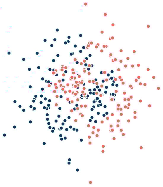
Figure 2. Example of dataset. Each colour represents a different class.

The objective is to reconstruct the original decision surface from this finite sample using the Lipschitz extension frameworks. We compare the performance of the McShane–Whitney mean extension ($F^{MW}$) and the Oberman–Milman extension ($F^{OM}$) under two distinct regimes: the direct extension of binary labels (Section 3.1) and the extension of smoothed probabilities (Section 3.2).

To implement the smoothing procedure defined in (8), we analyze the impact of two different decay kernels: the exponential decay $w_1$ and the power-law decay $w_2$:

$$w_1\left(t\right):=e^{-\lambda t},w_2\left(t\right):={(1+t)}^{-\lambda }.$$

(12)

In these experiments, the decay parameter $\lambda$ was determined based on the Silverman rule. While originally intended for density estimation, this rule provides a robust baseline for the kernel bandwidth designed to minimize the asymptotic mean integrated squared error. Since $\lambda$ acts as an inverse bandwidth, we set

$$\lambda ={\displaystyle \frac{\sqrt[5]{n}}{\sigma }},$$

where n is the number of observations (300) and $\sigma$ is the standard deviation of the dataset. This choice allows the smoothing scale to adapt automatically to the dispersion of the points, ensuring that the resulting Lipschitz extension captures the global topology of the data rather than fitting to local noise.

The reconstruction results are presented in Figure 3, Figure 4, Figure 5, Figure 6, Figure 7, Figure 8, Figure 9 and Figure 10. Several key observations can be derived from the visual comparison of the decision boundaries. The most prominent finding is the fundamental difference between the binary extensions and the smoothed versions. As seen in Figure 3 and Figure 6, applying the Lipschitz extension directly to the binary labels results in highly fragmented decision boundaries. This confirms our theoretical analysis regarding the uncertainty gap: without smoothing, the classifier rigidly adheres to local noise, producing “islands" of classes around outliers. This behavior is geometrically equivalent to the 1-Nearest Neighbour classifier, inheriting its high variance and susceptibility to overfitting. In contrast, the introduction of the kernel smoothing (Figure 4, Figure 5, Figure 7 and Figure 8) significantly improves the topological quality of the solution. The decision boundaries become continuous and smooth, successfully recovering the latent geometric structure of the central circular region and the separation boundary. This validates the result of Theorem 3, showing that the convolution with a log-Lipschitz kernel effectively regularizes the extension, reducing the Lipschitz constant of the input data and filtering out high-frequency noise.

Figure 3. McShane-Whitney extension without smoothing.

Figure 4. McShane-Whitney extension smoothed by $w_1$.

Figure 5. McShane-Whitney extension smoothed by $w_2$.

Figure 6. Oberman-Milman extension without smoothing.

Figure 7. Oberman-Milman extension smoothed by $w_1$.

Figure 8. Oberman-Milman extension smoothed by $w_2$.

Figure 9. Random forest.

Figure 10. Support Vector Machine.

The decision boundary of the Random Forest model (Figure 9) appears relatively sharp, which is indicative of its strength in handling complex patterns. However, it is evident that there is some overfitting in the central areas of the dataset. This is evident in the manner in which Random Forest tightly surrounds the few misclassified points, which suggests that it may be overly sensitive to localised variations. The SVM (Figure 10) offers a more gradual decision boundary; however, it also exhibits a similar tendency to Random Forest in failing to distinguish between classes, particularly in the more irregular regions. Naive Bayes (Figure 11) performs less well than the other classifiers, with a boundary that fails to capture the complexities of the dataset, resulting in larger regions where it misclassifies data points.

Figure 11. Naïve Bayes.

Comparing the exponential kernel ($w_1$) and the power-law kernel ($w_2$), we observe that both yield qualitatively similar results. This suggests that the proposed method is robust to the specific choice of the decay function, provided that the bandwidth parameter $\lambda$ is tuned to the data density. Both kernels successfully decoupled the inference from the local sampling artifacts, creating a stable decision surface.

It is important to note that, unlike “black box” models (such as neural networks or complex ensembles like Random Forest), our proposed methods remains fully interpretable. The classification of any new point x is explicitly derived from a distance-weighted aggregation of neighbours, followed by a bounded extension. Without hidden layers or opaque parameters, the decision logic is transparent and geometrically intuitive. This nature is particularly valuable when explaining the reasoning behind a prediction is as critical as accuracy. Furthermore, standard classifiers often lack guarantees on how the output changes with small input perturbations. In contrast, in our methods we can guarantee that a small perturbation in the input space will not cause a disproportionate jump in the predicted probability due to the control over the Lipschitz constant.

Overall, the experiments demonstrate that the combination of kernel smoothing with Lipschitz extensions (McShane–Whitney or Oberman–Milman) offers a superior balance between fidelity and regularity.

4.2. Backtesting

To assess the generalization capability of the proposed methods on real-world problems, we employed a diverse set of benchmark datasets [20,21,22,23]. These sources were selected to represent heterogeneous challenges, including unbalanced classes, high feature dimensionality, and small sample regimes. The experimental validation relied on 30 repeated random sub-sampling iterations to ensure statistical robustness. Moreover, the smoothing in the Lipschitz-based methods was conducted via the weight function $w_1$ presented in the previous section, with $\lambda =\sqrt[5]{n}{\sigma }^{-1}$. Performance was quantified using four standard metrics: Accuracy, F1 Score, Cross-Entropy (Log Loss), and ROC AUC. A standardized pre-processing was enforced, consisting of feature scaling and Principal Component Analysis (PCA) to preserve 90% of the variance. While ad hoc optimization for each dataset could improve individual scores, a unified processing was prioritized to ensure a rigorously comparable framework [24,25,26]. The resulting performance distributions are presented in the box plots below, from which key insights are derived.

In the rice dataset (Figure 12), the proposed Lipschitz-based methods demonstrate high competitiveness. The OM extension and SVM yield the highest median Accuracy and F1 Scores, significantly outperforming Naïve Bayes and exhibiting lower variance than Random Forest. In the probabilistic metrics, the MW method achieves the lowest Log Loss among all classifiers, indicating superior probability calibration. Furthermore, both MW and OM dominate the ROC AUC metric, surpassing SVM and Random Forest. This suggests that the Lipschitz extensions effectively preserve the global ranking structure of the classes within this specific metric topology.

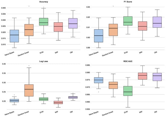
Figure 12. Performance for rice dataset.

The analysis of the breast cancer dataset (Figure 13) reveals a generally high performance ceiling, with most classifiers exceeding 95% accuracy. While SVM shows a slight advantage in accuracy and the lowest Log Loss, the MW extension remains very competitive, exhibiting a stability comparable to Random Forest (as evidenced by the compact interquartile ranges). A notable phenomenon is observed regarding the OM method: although it achieves high Accuracy, F1 and ROC AUC scores, it presents a significantly higher Log Loss compared to the other models. This indicates that while OM correctly identifies the decision boundary, it may be assigning overconfident probabilities to misclassified instances near the margin, whereas MW maintains a more conservative and robust probabilistic estimation.

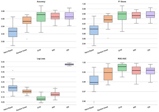
Figure 13. Performance for breast cancer dataset.

In the wine quality dataset (Figure 14), while Random Forest and SVM achieve the highest Accuracy, the OM method demonstrates exceptional performance in the ROC AUC metric, achieving a median score near 0.85, significantly higher than the SVM and MW (both below 0.75). This implies that the Oberman–Milman extension is particularly effective at distinguishing between classes across different decision thresholds, even if the default 0.5 cut-off does not maximize accuracy to the same extent as ensemble methods. Concurrently, MW reaffirms its probabilistic robustness with a competitive Log Loss, substantially outperforming Naïve Bayes.

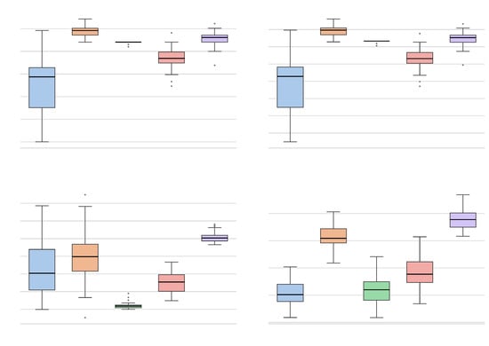
Figure 14. Performance for wine quality dataset.

Finally, in the spam dataset (Figure 15), characterized by higher dimensionality and feature sparsity, established methods like Random Forest and SVM show a slight superiority across metrics. However, MW and OM consistently outperform Naïve Bayes and maintain robust performance levels. This resilience suggests that the smoothing techniques integrated into the extensions effectively mitigate the influence of noise and outliers typical of spam detection tasks.

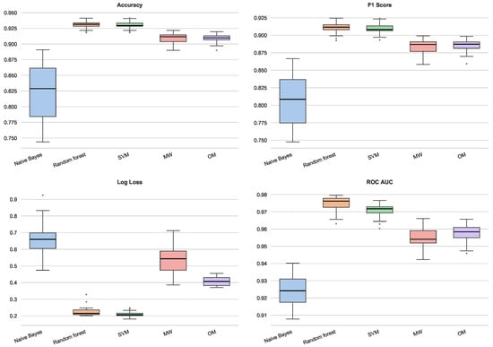
Figure 15. Performance for spam dataset.

In conclusion, these results indicate that the proposed Lipschitz extension frameworks are practical and competitive alternatives to state-of-the-art classifiers. While ensemble methods like Random Forest or kernel-based approaches like SVM may achieve marginal gains in performance in specific scenarios (the spam dataset), the proposed McShane–Whitney and Oberman–Milman offer a compelling advantage in terms of model parsimony and stability. Indeed, the hyperparameter tuning is limited to a single smoothing parameter $\lambda$, which can be effectively estimated from the data geometry, in contrast to the exhaustive grid searches required for SVM or Random Forest. Furthermore, the narrow interquartile ranges observed in the box plots indicate a high degree of robustness against sampling variations. This combination of stability, low configuration complexity, and geometric interpretability makes them a valuable alternative in classification problems. Notably, the MW extension consistently delivered superior probability calibration, evidenced by its competitive Log Loss scores, particularly in the rice and wine datasets. This suggests that the integration of kernel smoothing with Lipschitz constraints effectively filters local noise without sacrificing the global decision structure. Moreover, the OM method demonstrated a strong discriminative ability (high ROC AUC), proving effective even in complex topologies. Overall, the structural simplicity, combined with the observed low variance across experimental trials, suggests that Lipschitz-based classifiers provide a reliable and geometrically intuitive framework, especially suitable for domains where understanding the rationale behind a decision is as critical as the prediction itself.

References

- von Luxburg, U.; Bousquet, O. Distance-Based Classification with Lipschitz Functions. J. Mach. Learn. Res. 2004, 5, 669–695. [Google Scholar]
- Ioffe, S. Probabilistic Linear Discriminant Analysis; Springer: Berlin/Heidelberg, Germany, 2006; pp. 531–542. [Google Scholar]
- Gottlieb, L.A.; Kontorovich, A.; Krauthgamer, R. Efficient classification for metric data. IEEE Trans. Inf. Theory 2014, 60, 5750–5759. [Google Scholar] [CrossRef]
- Cranko, Z.; Shi, Z.; Zhang, X.; Nock, R.; Kornblith, S. Generalised Lipschitz regularisation equals distributional robustness. In Proceedings of the International Conference on Machine Learning, PMLR, Virtual Event, 18–24 July 2021; pp. 2178–2188. [Google Scholar]
- Petrov, A.; Eiras, F.; Sanyal, A.; Torr, P.H.S.; Bibi, A. Certifying ensembles: A general certification theory with S-Lipschitzness. arXiv 2023, arXiv:2304.13019. [Google Scholar] [CrossRef]
- Calabuig, J.M.; Falciani, H.; Sánchez-Pérez, E.A. Dreaming machine learning: Lipschitz extensions for reinforcement learning on financial markets. Neurocomputing 2020, 398, 172–184. [Google Scholar] [CrossRef]
- Falciani, H.; Sánchez-Pérez, E.A. Semi-Lipschitz functions and machine learning for discrete dynamical systems on graphs. Mach. Learn. 2022, 111, 1765–1797. [Google Scholar] [CrossRef]
- Arnau, R.; Calabuig, J.M.; Sánchez Pérez, E.A. Measure-Based Extension of Continuous Functions and p-Average-Slope-Minimizing Regression. Axioms 2023, 12, 359. [Google Scholar] [CrossRef]
- McShane, E.J. Extension of range of functions. Bull. Am. Math. Soc. 1934, 40, 837–842. [Google Scholar] [CrossRef]
- Whitney, H. Analytic extensions of differentiable functions defined in closed sets. Hassler Whitney Collect. Pap. 1992, 36, 228–254. [Google Scholar] [CrossRef]
- Mil’man, V.A. Lipschitz continuations of linearly bounded functions. Sb. Math. 1998, 189, 1179. [Google Scholar] [CrossRef]
- Oberman, A. An Explicit Solution of the Lipschitz Extension Problem. Proc. Am. Math. Soc. 2008, 136, 4329–4338. [Google Scholar] [CrossRef]
- Aliprantis, C.; Border, K.C. Infinite Dimensional Analysis: A Hitchhiker’s Guide; Springer: Berlin/Heidelberg, Germany, 1999. [Google Scholar]
- Hastie, T.; Tibshirani, R.; Friedman, J. The Elements of Statistical Learning. Data Mining, Inference, and Prediction; Springer: Berlin/Heidelberg, Germany, 2009. [Google Scholar]
- Nadaraya, E.A. On estimating regression. Theory Probab. Its Appl. 1964, 9, 141–142. [Google Scholar] [CrossRef]
- Watson, G.S. Smooth regression analysis. Sankhyā Indian J. Stat. Ser. A 1964, 26, 359–372. [Google Scholar]
- Rockafellar, R.T. Convex Analysis; Princeton University Press: Princeton, NJ, USA, 2015. [Google Scholar]
- Fazlyab, M.; Robey, A.; Hassani, H.; Morari, M.; Pappas, G. Efficient and accurate estimation of lipschitz constants for deep neural networks. In Advances in Neural Information Processing Systems; Curran Associates Inc.: Red Hook, NY, USA, 2019; Volume 32. [Google Scholar]
- Deng, G.; Manton, J.H.; Wang, S. Fast kernel smoothing by a low-rank approximation of the kernel toeplitz matrix. J. Math. Imaging Vis. 2018, 60, 1181–1195. [Google Scholar] [CrossRef]
- Rice (Cammeo and Osmancik). UCI Machine Learning Repository. 2019. Available online: https://archive.ics.uci.edu/dataset/545/rice+cammeo+and+osmancik (accessed on 16 December 2025).
- Wolberg, W.H.; Mangasarian, O.L.; Street, W.N. Breast Cancer Wisconsin (Diagnostic). UCI Machine Learning Repository. 1995. Available online: https://archive.ics.uci.edu/dataset/17/breast+cancer+wisconsin+diagnostic (accessed on 16 December 2025).
- Cortez, P.; Cerdeira, A.; Almeida, F.; Matos, T.; Reis, J. Wine Quality. UCI Machine Learning Repository. 2009. Available online: https://archive.ics.uci.edu/dataset/186/wine+quality (accessed on 16 December 2025).
- Hopkins, M.; Reeber, E.; Forman, G.; Suermondt, J. Spambase. UCI Machine Learning Repository. 1999. Available online: https://archive.ics.uci.edu/dataset/94/spambase (accessed on 16 December 2025).
- Grandini, M.; Bagli, E.; Visani, G. Metrics for multi-class classification: An overview. arXiv 2020, arXiv:2008.05756. [Google Scholar] [CrossRef]
- Hossin, M.; Sulaiman, M.N. A review on evaluation metrics for data classification evaluations. Int. J. Data Min. Knowl. Manag. Process 2015, 5, 1. [Google Scholar]
- Van Der Maaten, L.; Postma, E.O.; Van Den Herik, H.J. Dimensionality reduction: A comparative review. J. Mach. Learn. Res. 2009, 10, 13. [Google Scholar]
Disclaimer/Publisher’s Note: The statements, opinions and data contained in all publications are solely those of the individual author(s) and contributor(s) and not of MDPI and/or the editor(s). MDPI and/or the editor(s) disclaim responsibility for any injury to people or property resulting from any ideas, methods, instructions or products referred to in the content. |
© 2026 by the authors. Licensee MDPI, Basel, Switzerland. This article is an open access article distributed under the terms and conditions of the Creative Commons Attribution (CC BY) license.