Constrained Quantization for Probability Distributions

Abstract

In this work, we extend the classical framework of quantization for Borel probability measures defined on normed spaces ${\mathbb{R}}^k$ by introducing and analyzing the notions of the nth constrained quantization error, constrained quantization dimension, and constrained quantization coefficient. These concepts generalize the well-established nth quantization error, quantization dimension, and quantization coefficient, which are traditionally considered in the unconstrained setting and thereby broaden the scope of quantization theory. A key distinction between the unconstrained and constrained frameworks lies in the structural properties of optimal quantizers. In the unconstrained setting, if the support of P contains at least n elements, then the elements of an optimal set of n-points coincide with the conditional expectations over their respective Voronoi regions; this characterization does not, in general, persist under constraints. Moreover, it is known that if the support of P contains at least n elements, then any optimal set of n-points in the unconstrained case consists of exactly n distinct elements. This property, however, may fail to hold in the constrained context. Further differences emerge in asymptotic behaviors. For absolutely continuous probability measures, the unconstrained quantization dimension is known to exist and equals the Euclidean dimension of the underlying space. In contrast, we show that this equivalence does not necessarily extend to the constrained setting. Additionally, while the unconstrained quantization coefficient exists and assumes a unique, finite, and positive value for absolutely continuous measures, we establish that the constrained quantization coefficient can exhibit significant variability and may attain any nonnegative value, depending critically on the specific nature of the constraint applied to the quantization process.

1. Introduction

The most common form of quantization is rounding-off. Its purpose is to reduce the cardinality of the representation space, particularly when the input data is real-valued. It has broad applications in communications, information theory, signal processing, and data compression (see [1,2,3,4,5,6,7,8]). For $k\in \mathbb{N}$, where $\mathbb{N}$ is the set of natural numbers, let d be a metric induced by a norm $\parallel ·\parallel$ on ${\mathbb{R}}^k$. Let P be a Borel probability measure on ${\mathbb{R}}^k$ and $r\in (0,\infty )$. Let S be a nonempty closed subset of ${\mathbb{R}}^k$ and $\alpha \subseteq S$ be a locally finite (i.e., the intersection of $\alpha$ with any bounded subset of ${\mathbb{R}}^k$ is finite) subset of ${\mathbb{R}}^k$. This implies that $\alpha$ is countable and closed. Then, the distortion error for P, of order r, with respect to the set $\alpha \subseteq S$, denoted by $V_r(P;\alpha )$, is defined by

$$V_r(P;\alpha )=\int \underset{a\in \alpha }{min}d{(x,a)}^{r}dP\left(x\right).$$

Then, for $n\in \mathbb{N}$, the nth constrained quantization error for P, of order r, with respect to the set S, is defined by

$$V_{n,r}:=V_{n,r}\left(P\right)=inf\left\{V_r(P;\alpha ):\alpha \subseteq S,1\le \mathrm{card}\left(\alpha \right)\le n\right\},$$

(1)

where $\mathrm{card}\left(A\right)$ represents the cardinality of a set A. If, in the definition of the nth constrained quantization error, the set S, known as constraint, is chosen as the set ${\mathbb{R}}^k$ itself, then the nth constrained quantization error is referred to as the nth unconstrained quantization error, which in the literature is traditionally referred to as the nth quantization error. For some recent work in the direction of unconstrained quantization, one can see [9,10,11,12,13,14,15,16,17,18,19]. For the probability measure P, we assume that

$$\int d{(x,0)}^{r}dP\left(x\right)<\infty .$$

(2)

A set $\alpha$, for which the infimum in (1) exists and does not contain more than n elements, is called a constrained optimal set of n-points for P with respect to the constraint S. The collection of all optimal sets of n-points for P with respect to the constraint S is denoted by ${\mathcal{C}}_{n,r}(P;S)$.

Proposition 1.

Let the assumption (2) be true. Then, $V_{n,r}\left(P\right)$ exists and is a decreasing sequence of finite nonnegative numbers.

Proof. 

Assume that condition (2) holds, i.e.,

$$\int d{(x,0)}^{r}dP\left(x\right)<\infty .$$

We first show that this implies

$$\int d{(x,a)}^{r}dP\left(x\right)<\infty \mathrm{for}\mathrm{every}a\in {\mathbb{R}}^k.$$

By the triangle inequality, we have

$$d(x,a)\le d(x,0)+d(0,a)\le 2max\left\{d\right(x,0),d(0,a\left)\right\}.$$

Raising both sides to the power r (where $0<r<\infty$) yields

$$d{(x,a)}^r\le 2^{r}max\{d{(x,0)}^r,d{(0,a)}^r\}\le 2^r\left(d{(x,0)}^r+d{(0,a)}^r\right).$$

Integrating with respect to P, we obtain

$$\int d{(x,a)}^{r}dP\left(x\right)\le 2^r\left(\int d{(x,0)}^{r}dP\left(x\right)+d{(0,a)}^r\right)<\infty$$

since the first integral is finite by (2) and $d{(0,a)}^r$ is a finite constant. Hence,

$$\int d{(x,a)}^{r}dP\left(x\right)<\infty \mathrm{for}\mathrm{all}a\in {\mathbb{R}}^k.$$

(⭑)

Now, let $\alpha \subseteq S\subseteq {\mathbb{R}}^k$ be any nonempty finite set, and consider

$$V_r(P;\alpha )=\int \underset{a\in \alpha }{min}d{(x,a)}^{r}dP\left(x\right).$$

Since ${min}_{a\in \alpha }d{(x,a)}^r\ge 0$, we have $V_r(P;\alpha )\ge 0$. Moreover, for any fixed $a_0\in \alpha$, we have

$$\underset{a\in \alpha }{min}d{(x,a)}^r\le d{(x,a_0)}^r.$$

Therefore, using $(⭑)$, we have

$$0\le V_r(P;\alpha )=\int \underset{a\in \alpha }{min}d{(x,a)}^{r}dP\left(x\right)\le \int d{(x,a_0)}^{r}dP\left(x\right)<\infty .$$

Thus, every admissible finite set $\alpha$ yields a finite nonnegative value of $V_r(P;\alpha )$.

Consequently, when we define

$$V_{n,r}\left(P\right)=inf\left\{V_r(P;\alpha ):\alpha \subseteq S,1\le \mathrm{card}\left(\alpha \right)\le n\right\},$$

the infimum is taken over a nonempty collection of finite nonnegative numbers. Hence,

$$0\le V_{n,r}\left(P\right)<\infty ,$$

showing that $V_{n,r}\left(P\right)$ exists as a finite nonnegative number.

Finally, the monotonicity follows immediately from the definition. If $m>n$, then

$$\{\alpha \subseteq S:1\le \mathrm{card}(\alpha )\le n\}\subseteq \{\alpha \subseteq S:1\le \mathrm{card}(\alpha )\le m\},$$

so taking infima over larger sets cannot increase the value. Therefore,

$$V_{m,r}\left(P\right)\le V_{n,r}\left(P\right),$$

and thus ${\left\{V_{n,r}\left(P\right)\right\}}_{n\ge 1}$ is a decreasing sequence. This completes the proof. □

Remark 1.

The moment condition (2) is being assumed throughout this paper.

The following two propositions reflect two important properties of constrained quantization.

Proposition 2.

In constrained quantization for any Borel probability measure P, an optimal set of one-point always exists, i.e., ${\mathcal{C}}_{1,r}(P;S)$ is nonempty.

Proof. 

Let $0<r<\infty$. Define a function

$${\psi }_r:S\to {\mathbb{R}}^{+}:{\psi }_r\left(a\right)=\int d{(x,a)}^{r}dP\left(x\right).$$

The function ${\psi }_r$ is, obviously, continuous. Then, for every $c\in {\mathbb{R}}^{+}$ with

$$c>\underset{b\in S}{inf}\int d{(x,b)}^{r}dP\left(x\right),$$

the level sets

$$\{{\psi }_r\le c\}:=\{a\in S:\int d{(x,a)}^{r}dP\left(x\right)\le c\}$$

are closed subsets of S. Proceeding in a similar way, as shown in the previous proposition, for any $0<r<\infty$, we have

$$\begin{array}{c}\hfill d{(0,a)}^r\le 2^r\left(d{(x,a)}^r+d{(x,0)}^r\right).\end{array}$$

Thus, for $a\in \{{\psi }_r\le c\}$, we have

$$\begin{array}{cc}\hfill d{(0,a)}^r=\int d{(0,a)}^{r}dP\left(x\right)& \le 2^r\left(\int (d{(x,a)}^r+d{(x,0)}^r)dP\left(x\right)\right)\le 2^r\left(c+{E\parallel X\parallel }^r\right),\hfill \end{array}$$

i.e.,

$$d(0,a)\le 2{\left(c+{E\parallel X\parallel }^r\right)}^{{\displaystyle \frac{1}{r}}}\mathrm{yielding}\{{\psi }_r\le c\}\subseteq B\left(0,2{\left(c+{E\parallel X\parallel }^r\right)}^{{\displaystyle \frac{1}{r}}}\right),$$

where ${E\parallel X\parallel }^r=\int d{(x,0)}^{r}dP\left(x\right)$. Hence, the level sets are bounded. As the level sets are both bounded and closed, they are compact. Let us now consider a decreasing sequence $\left\{c_n\right\}$ of elements in ${\mathbb{R}}^{+}$ such that

$$c_n>\underset{b\in S}{inf}\int d{(x,b)}^{r}dP\left(x\right)\mathrm{and}{c}_n\to \underset{b\in S}{inf}\int d{(x,b)}^{r}dP\left(x\right).$$

(3)

Then,

$$\{a\in S:\int d{(x,a)}^{r}dP\left(x\right)\le c_{n+1}\}\subseteq \{a\in S:\int d{(x,a)}^{r}dP\left(x\right)\le c_n\},\mathrm{i}.\mathrm{e}.,$$

$$\{{\psi }_r\le c_{n+1}\}\subseteq \{{\psi }_r\le c_n\}.$$

Also, $\{{\psi }_r\le c_n\}\ne \varnothing$ for all $n\in \mathbb{N}$. If this is not true, then there will exist an element $c_N$ for some $N\in \mathbb{N}$ such that, for all $b\in S$, we have

$$c_N<\int d{(x,b)}^{r}dP\left(x\right)\mathrm{yielding}{c}_N\le \underset{b\in S}{inf}\int d{(x,b)}^{r}dP\left(x\right),$$

which contradicts (3). Thus, we see that the level sets $\{{\psi }_r\le c_n\}$ form a nested sequence of nonempty compact sets. Hence,

$$\bigcap _{n=1}^{\infty }\{{\psi }_r\le c_n\}\ne \varnothing .$$

Let $a\in {\displaystyle \bigcap _{n=1}^{\infty }}\{{\psi }_r\le c_n\}$. Then,

$$\underset{b\in S}{inf}\int d{(x,b)}^{r}dP\left(x\right)\le \int d{(x,a)}^{r}dP\left(x\right)<c_n\mathrm{for}\mathrm{all}n\in \mathbb{N},$$

which, by squeeze theorem, implies that

$$\underset{b\in S}{inf}\int d{(x,b)}^{r}dP\left(x\right)=\int d{(x,a)}^{r}dP\left(x\right),$$

i.e., $\left\{a\right\}$ forms an optimal set of one-point, i.e., $\left\{a\right\}\in {\mathcal{C}}_{1,r}(P;S)$, i.e., ${\mathcal{C}}_{1,r}(P;S)$ is nonempty. Thus, the proof of the proposition is complete. □

Definition 1.

Let P be a Borel probability measure on ${\mathbb{R}}^k$, and let U be the largest open subset of ${\mathbb{R}}^k$ such that $P\left(U\right)=0$. Then, ${\mathbb{R}}^k\setminus U$ is called the support of P, and it is denoted by $supp\left(P\right)$. For a locally finite set $\alpha \subseteq {\mathbb{R}}^k$—and $a\in \alpha$—by $M\left(a\right|\alpha )$, we denote the set of all elements in ${\mathbb{R}}^k$ which are nearest to a among all the elements in α, i.e.,

$$M\left(a\right|\alpha )=\{x\in {\mathbb{R}}^k:d(x,a)=\underset{b\in \alpha }{min}d(x,b)\}.$$

$M\left(a\right|\alpha )$ is called the Voronoi region in ${\mathbb{R}}^k$ generated by $a\in \alpha$. The set $\left\{M\right(a\left|\alpha \right):a\in \alpha \}$ is called the Voronoi diagram or Voronoi tessellation of ${\mathbb{R}}^k$ with respect to the set α. Further, for $\alpha =\{a_1,a_2,\dots \}\subseteq S$, let us define the sets $A_{a_i|\alpha }$ for $a_i\in \alpha$ as follows:

$$\begin{array}{c}\hfill A_{a_i|\alpha }=\left\{\begin{array}{cc}M\left(a_1\right|\alpha )\hfill & ifi=1,\hfill \\ M\left(a_i\right|\alpha )\setminus \bigcup _{k<i}M\left(a_k\right|\alpha )\hfill & ifi\ge 2.\hfill \end{array}\right.\end{array}$$

(4)

The set $\{A_{a_i|\alpha }:a_i\in \alpha \}$ is called the Voronoi partition of ${\mathbb{R}}^k$ with respect to the set α (and S).

Proposition 3.

Let P be a Borel probability measure on ${\mathbb{R}}^k$ and let S be a nonempty closed subset of ${\mathbb{R}}^k$. Let ${\alpha }_n$ be an optimal set of n-points for P with respect to the constraint S. Then, ${\alpha }_n$ contains exactly n elements if and only if there exists a set $\alpha \subseteq S$ containing at least n elements such that

$$P\left(A_{a|\alpha }\right)>0foreacha\in \alpha .$$

Proof. 

Let us first assume that there exists a set $\alpha \subseteq S$ containing at least n elements such that

$$P\left(A_{a|\alpha }\right)>0\mathrm{for}\mathrm{each}a\in \alpha .$$

If $n=1$, then the proposition is a consequence of Proposition 2. Let us now prove the proposition for $2\le n$. For the sake of contradiction, assume that $\gamma :=\{b_1,b_2,\dots ,b_m\}\subseteq S$ is an optimal set of n-points for P, such that $\mathrm{card}\left(\gamma \right)=m$ for some positive integer $m<n$, i.e.,

$$V_{n,r}\left(P\right)=\int \underset{a\in \gamma }{min}d{(x,a)}^{r}dP\left(x\right).$$

If $m\ge 2$, then we have

$$V_{n,r}\left(P\right)=\sum _{j=1}^m{\int }_{A_{b_j|\gamma }}d{(x,b_j)}^{r}dP\left(x\right).$$

Since $\mathrm{card}\left(\alpha \right)>\mathrm{card}\left(\gamma \right)$, let $c\in \alpha$ be such that $c\notin \{b_j:1\le j\le m\}$. Then, $c\in A_{b_{\ell }|\gamma }$ for some $1\le \ell \le m$. Consider the set $\gamma \cup \left\{c\right\}$, then we can write

$$\gamma \cup \left\{c\right\}=\{b_1,b_2,\cdots ,b_m,b_{m+1}\},\mathrm{where}{b}_{m+1}=c.$$

Notice that $A_{c|\gamma \cup \{c\}}$ intersects some of the Voronoi partitions of $A_{b_j|\gamma }$ for $1\le j\le m$. If $A_{c|\gamma \cup \{c\}}$ does not intersect $A_{b_j|\gamma }$ for some $1\le j\le m$, then

$$\begin{array}{c}\hfill {\int }_{A_{b_j|\gamma }}d{(x,b_j)}^{r}dP\left(x\right)={\int }_{A_{b_j|\gamma \cup \left\{c\right\}}}d{(x,b_j)}^{r}dP\left(x\right).\end{array}$$

(5)

On the other hand, if $A_{c|\gamma \cup \{c\}}$ intersects $A_{b_j|\gamma }$ for some $1\le j\le m$, then

$$\begin{array}{cc}\hfill & {\int }_{A_{b_j|\gamma }}d{(x,b_j)}^{r}dP\left(x\right)\hfill \\ \hfill =& {\int }_{A_{b_j|\gamma }\cap A_{c|\gamma \cup \{c\}}}d{(x,b_j)}^{r}dP\left(x\right)+{\int }_{A_{b_j|\gamma }\cap A_{c|\gamma \cup \{c\}}^c}d{(x,b_j)}^{r}dP\left(x\right)\hfill \\ \hfill >& {\int }_{A_{b_j|\gamma }\cap A_{c|\gamma \cup \{c\}}}d{(x,c)}^{r}dP\left(x\right)+{\int }_{A_{b_j|\gamma }\cap A_{c|\gamma \cup \{c\}}^c}d{(x,b_j)}^{r}dP\left(x\right).\hfill \end{array}$$

(6)

For $1\le t<m$, let $A_{c|\gamma \cup \{c\}}$ intersect $A_{b_{{\ell }_i}|\gamma }$, where $b_{{\ell }_i}\in \{b_j:1\le j\le m\}$ for $i\in \{1,2,\cdots t\}$. Then,

$$A_{c|\gamma \cup \{c\}}=\bigcup _{i=1}^t{A}_{b_{{\ell }_i}|\gamma }\cap A_{c|\gamma \cup \{c\}}.$$

Hence, by the expressions in (5) and (6), we have

$$\begin{array}{cc}\hfill V_{n,r}\left(P\right)=& \int \underset{a\in \gamma }{min}d{(x,a)}^{r}dP\left(x\right)\hfill \\ \hfill >& \sum _{j\in (\{1,2,\cdots ,m\}\setminus \{{\ell }_1,{\ell }_2,\cdots ,{\ell }_t\})}{\int }_{A_{b_j|\gamma \cup \left\{c\right\}}}d{(x,b_j)}^{r}dP\left(x\right)\hfill \\ \hfill & +\sum _{i=1}^t\left({\int }_{A_{b_{{\ell }_i}|\gamma }\cap A_{c|\gamma \cup \{c\}}}d{(x,c)}^{r}dP\left(x\right)+{\int }_{A_{b_{{\ell }_i}|\gamma }\cap A_{c|\gamma \cup \{c\}}^c}d{(x,b_{{\ell }_i})}^{r}dP\left(x\right)\right)\hfill \\ \hfill =& \sum _{j\in (\{1,2,\cdots ,m\}\setminus \{{\ell }_1,{\ell }_2,\cdots ,{\ell }_t\})}{\int }_{A_{b_j|\gamma \cup \left\{c\right\}}}d{(x,b_j)}^{r}dP\left(x\right)+{\int }_{A_{c|\gamma \cup \{c\}}}d{(x,c)}^{r}dP\left(x\right)\hfill \\ \hfill & +\sum _{i=1}^t{\int }_{A_{b_{{\ell }_i}|\gamma }\cap A_{c|\gamma \cup \{c\}}^c}d{(x,b_{{\ell }_i})}^{r}dP\left(x\right)\hfill \\ \hfill =& \sum _{j\in (\{1,2,\cdots ,m\}\setminus \{{\ell }_1,{\ell }_2,\cdots ,{\ell }_t\})}{\int }_{A_{b_j|\gamma \cup \left\{c\right\}}}d{(x,b_j)}^{r}dP\left(x\right)+{\int }_{A_{c|\gamma \cup \{c\}}}d{(x,c)}^{r}dP\left(x\right)\hfill \\ \hfill & +\sum _{i=1}^t{\int }_{A_{b_{{\ell }_i}|\gamma \cup \left\{c\right\}}}d{(x,b_{{\ell }_i})}^{r}dP\left(x\right)\hfill \\ \hfill =& \int \underset{a\in \gamma \cup \left\{c\right\}}{min}d{(x,a)}^{r}dP\left(x\right)\ge V_{n,r}\left(P\right),\hfill \end{array}$$

where the last inequality is true since $\gamma \cup \left\{c\right\}$ contains no more than n elements. Thus, we see that a contradiction arises. Hence, an optimal set of n-points contains exactly n elements.

Next, assume that ${\alpha }_n$ is an optimal set of n-points for P with respect to the constraint S such that ${\alpha }_n$ contains exactly n elements. We need to show that

$$P\left(A_{a|{\alpha }_n}\right)>0\mathrm{for}\mathrm{each}a\in {\alpha }_n.$$

For the sake of contradiction, let $\gamma$ be the nonempty maximal subset of ${\alpha }_n$ such that $P\left(A_{b|{\alpha }_n}\right)=0\mathrm{for}\mathrm{each}b\in \gamma$ and $P\left(A_{b|{\alpha }_n}\right)>0\mathrm{for}\mathrm{each}b\in {\alpha }_n\setminus \gamma$. Since the optimal set of one-point always exists, then $\gamma \ne {\alpha }_n$. Let $\mathrm{card}\left(\gamma \right)=m$, and then $\mathrm{card}({\alpha }_n\setminus \gamma )=n-m$. Thus, we see that

$$\begin{array}{cc}\hfill V_{n,r}\left(P\right)& =\int \underset{a\in {\alpha }_n}{min}d{(x,a)}^{r}dP\left(x\right)=\sum _{a\in {\alpha }_n}{\int }_{A_{a|{\alpha }_n}}d{(x,a)}^{r}dP\left(x\right)\hfill \\ \hfill =& \sum _{a\in {\alpha }_n\setminus \gamma }{\int }_{A_{a|{\alpha }_n\setminus \gamma }}d{(x,b)}^{r}dP\left(x\right),\hfill \end{array}$$

which implies that ${\alpha }_n\setminus \gamma$ is an optimal set of n-points such that $\mathrm{card}({\alpha }_n\setminus \gamma )=n-m<n$, which contradicts our assumption. Thus, we see that, if ${\alpha }_n$ is an optimal set of n-points containing exactly n elements, then

$$P\left(A_{a|{\alpha }_n}\right)>0\mathrm{for}\mathrm{each}a\in {\alpha }_n.$$

Thus, the proof of the proposition is complete. □

The following corollaries are direct consequences of Proposition 3.

Corollary 1.

Let P be a Borel probability measure on ${\mathbb{R}}^k$ and let S be a nonempty closed subset of ${\mathbb{R}}^k$ such that there exists a set $\alpha \subseteq S$ containing at least N elements for some positive integer N such that

$$P\left(A_{a|\alpha }\right)>0foreacha\in \alpha .$$

Then, the sequence ${\left\{V_{n,r}\left(P\right)\right\}}_{n=1}^N$ is strictly decreasing, i.e., $V_{n-1,r}\left(P\right)>V_{n,r}\left(P\right)$ for all $2\le n\le N$, where $V_{n,r}\left(P\right)$ represents the nth constrained quantization error with respect to the constraint S.

Corollary 2.

Let P be a Borel probability measure on ${\mathbb{R}}^k$ and S be a nonempty closed subset of ${\mathbb{R}}^k$. Let α be an optimal set of n-points containing exactly n elements for P with respect to the constraint S and $a\in \alpha$. Then, $P\left(M\right(a\left|\alpha \right))>0$.

Although the following proposition has already been established in [3], we provide an alternative proof based on Proposition 3.

Proposition 4.

Let P be a Borel probability measure on ${\mathbb{R}}^k$, if $S={\mathbb{R}}^k$, i.e., when there is no constraint, then an optimal set of n-points for P contains exactly n elements if and only if the $supp\left(P\right)$ contains al least n elements.

Proof. 

If an optimal set of n-points contains exactly n elements, then it is easy to observe that $\mathrm{supp}\left(P\right)\ge n$. Next, assume that $\mathrm{supp}\left(P\right)\ge n$. We need to prove that an optimal set of n-points for P contains exactly n elements. In view of Proposition 3, it is sufficient to prove that there exists a subset $\alpha \subseteq {\mathbb{R}}^k$ containing at least n elements such that $P\left(A_{a|\alpha }\right)>0$ for all $a\in \alpha$. For the sake of contradiction, let $\gamma =\{a_1,a_2,\dots a_m\}\subseteq {\mathbb{R}}^k$ be a subset of maximal element $m<n$ such that $P\left(A_{a_i|\gamma }\right)>0$ for all $a_i\in \gamma$. Since $\mathrm{supp}\left(P\right)\ge n$, there exists $b\in \mathrm{supp}\left(P\right)$ with $b\notin \gamma$ such that $b\in A_{a_{\ell }|\gamma }$ for some $1\le \ell \le m$. Then, proceeding analogously as the proof of Proposition 3, we can prove that $\gamma \cup \left\{b\right\}$ is a set of $m+1$ elements such that $P\left(A_{a|\gamma \cup \{b\}}\right)>0$ for all $a\in \gamma \cup \left\{b\right\}$, which gives a contradiction. Thus, we can deduce that an optimal set of n-points contains exactly n elements. Hence, the proof of the proposition is complete. □

The following proposition is a standard result in quantization theory (see [3]). However, for the sake of completeness, we provide a proof here.

Proposition 5.

Let P be a Borel probability measure on ${\mathbb{R}}^k$. If $S={\mathbb{R}}^k$, i.e., when there is no constraint, then the elements in an optimal set of n-points are the conditional expectations in their own Voronoi regions provided that the $supp\left(P\right)$ contains at least n elements.

Proof. 

Let ${\alpha }_n$ be an optimal set of n-points for P and let $\{A_{a|{\alpha }_n}:a\in {\alpha }_n\}$ be the Voronoi partition of ${\mathbb{R}}^k$ with respect to the set ${\alpha }_n$. Let $V_{n,r}\left(P\right)$ be the corresponding nth quantization error. Then,

$$\begin{array}{c}\hfill V_{n,r}\left(P\right)=\int \underset{a\in {\alpha }_n}{min}d{(x,a)}^{r}dP\left(x\right)=\sum _{a\in {\alpha }_n}{\int }_{A_{a|{\alpha }_n}}d{(x,a)}^{r}dP\left(x\right).\end{array}$$

Notice that $V_{n,r}\left(P\right)$ will be minimum if the function

$${\mathsf{F}}_r\left(a\right):={\int }_{A_{a|{\alpha }_n}}d{(x,a)}^{r}dP\left(x\right)$$

is minimum for each $a\in {\alpha }_n$. Notice that the value of a—where the function $F_r\left(a\right)$ is minimum—does not depend on r because, for any $u,v,w,z\in {\mathbb{R}}^k$, and $r>0$, we have

$$\begin{array}{c}\hfill d(u,v)\le d(w,z)\mathrm{if}\mathrm{and}\mathrm{only}\mathrm{if}d{(u,v)}^r\le d{(w,z)}^r.\end{array}$$

Hence, for simplicity, we calculate the value of a, where $F_r\left(a\right)$ is minimum, for $r=2$. For this, we first compute the gradient $\nabla {\mathsf{F}}_2\left(a\right)$. We have

$$\begin{array}{cc}\hfill \nabla {\mathsf{F}}_2\left(a\right)={\displaystyle \frac{d}{da}}{\int }_{A_{a|{\alpha }_n}}d{(x,a)}^{2}dP\left(x\right)=& {\displaystyle \frac{d}{da}}{\int }_{A_{a|{\alpha }_n}}{\parallel x-a\parallel }^{2}dP\left(x\right)\hfill \\ \hfill =& {\int }_{A_{a|{\alpha }_n}}{\nabla }_a{\parallel x-a\parallel }^{2}dP\left(x\right).\hfill \end{array}$$

Since,

$${\nabla }_a{\parallel x-a\parallel }^2={\nabla }_a\left[{(x-a)}^T(x-a)\right]=-2(x-a),$$

where $x^T$ gives the transpose of $x\in {\mathbb{R}}^k$, we have

$$\nabla {\mathsf{F}}_2\left(a\right)={\int }_{A_{a|{\alpha }_n}}-2(x-a)dP\left(x\right)=-2\left({\int }_{A_{a|{\alpha }_n}}xdP\left(x\right)-a·P\left(A_{a|{\alpha }_n}\right)\right).$$

Set this to zero to find the minimizer:

$$-2\left({\int }_{A_{a|{\alpha }_n}}xdP\left(x\right)-a·P\left(A_{a|{\alpha }_n}\right)\right)=0.$$

Solve for a to obtain:

$$a={\displaystyle \frac{1}{P\left(A_{a|{\alpha }_n}\right)}}{\int }_{A_{a|{\alpha }_n}}xdP\left(x\right)=E(X\mid X\in A_{a|{\alpha }_n}).$$

Hence, the elements in an optimal set of n-points are the conditional expectations in their own Voronoi regions. Thus, the proof of the proposition is complete. □

Remark 2.

Let P be a Borel probability measure on ${\mathbb{R}}^k$ and let S be a nonempty closed subset of ${\mathbb{R}}^k$. Let α be an optimal set of n-points for P with respect to the constraint S and $a\in \alpha$. If the probability measure P is absolutely continuous with respect to the Lebesgue measure on ${\mathbb{R}}^k$, then it is easy to observe that $P(\partial M(a\left|\alpha \right))=0$, where $\partial M\left(a\right|\alpha )$ represents the boundary of the Voronoi region $M\left(a\right|\alpha )$. However, when P is not absolutely continuous, this property may fail, even in constrained quantization, as shown in the following example.

Example 1.

Let P be a Borel probability measure on $\mathbb{R}$ which is discrete and uniform on its support $\{1,2,3,4,5,6,7\}$. Let us take the constraint as

$$S=\left\{\right(2.5,1),(5.5,1\left)\right\}\cup \left\{\right(x,1):x\in \mathbb{R}\mathit{and}x\ge 12\}.$$

Let ${\alpha }_n$ denote a constrained optimal set of n-points with respect to the constraint S for the probability distribution P. Then, we have

$$\begin{array}{cc}\hfill {\alpha }_1& =\left\{(2.5,1)\right\},or\left\{(5.5,1)\right\},and{\alpha }_2=\{(2.5,1),(5.5,1)\}.\hfill \end{array}$$

Write $a_1=(2.5,1)$ and $a_2=(5.5,1)$. Then, notice that $P(\partial M\left(a_1\right|{\alpha }_2))=P(\partial M\left(a_2\right|{\alpha }_2))=P\left(\left\{4\right\}\right)={\displaystyle \frac{1}{7}}\ne 0$, exactly as intended.

In view of Proposition 5, in the case of unconstrained quantization, the elements in an optimal set are the conditional expectations in their own Voronoi regions. However, as will be demonstrated in later sections, this characterization does not generally hold in the context of constrained quantization. Because of that, in the case of constrained quantization, a set $\alpha$ for which the infimum in (1) exists and contains no more than n elements is called an optimal set of n-points instead of calling it an optimal set of n-means. Elements of an optimal set are called optimal elements. In unconstrained quantization, as described in [3], if the support of P contains at least n elements, then an optimal set of n-means always contains exactly n elements. However, this property does not carry over to constrained quantization. In particular, while an optimal set of one-point containing exactly one element in the constrained setting always exists, an optimal set of n-points containing exactly n elements for $n\ge 2$ may not exist, even if the support of P has at least n elements. Notice that unconstrained quantization, as described in [3], is a special case of constrained quantization. Nonetheless, there are some properties that hold in the unconstrained case, and they do not extend to the constrained setting.

This paper deals with $r=2$, $k=2$, and the metric on ${\mathbb{R}}^2$ as the Euclidean metric induced by the Euclidean norm $\parallel ·\parallel$. Instead of writing $V_r(P;\alpha )$ and $V_{n,r}:=V_{n,r}\left(P\right)$, we will write them as $V(P;\alpha )$ and $V_n:=V_n\left(P\right)$, i.e., r is omitted in the subscript as $r=2$ throughout this paper.

1.1. Motivation and Work Done

There are several research works in the literature on unconstrained quantization (see, for instance, [2,3,4,5,6,7,8,14,15,16,17,18,19]), and it has proven effective in solving problems for various probability distributions, such as uniform and self-similar distributions. However, in many real-life situations, quantization is subject to spatial or geometric restrictions.

A key motivating example arises in radiation therapy planning. In such applications, radiation beams or sampling points cannot be placed arbitrarily in space; instead, they must avoid sensitive or healthy tissue. Mathematically, this restriction can be modeled by introducing a constraint set $S\subset {\mathbb{R}}^k$ representing the admissible region, where quantizer points are allowed to lie. The complement ${\mathbb{R}}^k\setminus S$ can then be interpreted as a forbidden region, corresponding to organs or tissue that must not be directly exposed to radiation. Consequently, the optimization problem becomes one of minimizing the quantization error subject to the requirement that all optimal elements lie in S.

This naturally leads to the notion of constrained quantization, where the locations of optimal quantizer points are restricted by geometric, physical, or safety considerations. In this paper, we introduce and analyze constrained quantization for probability distributions by defining the constrained quantization error, constrained quantization dimension, and constrained quantization coefficient. We further compute optimal sets of n-points for several distributions under different constraint geometries, illustrating how constraints significantly alter both optimal configurations and asymptotic behavior.

To make the theoretical consequences of constrained quantization concrete, we focus on geometrically simple yet structurally informative model cases—such as uniform distributions supported on a line segment, a circle, and a chord—together with natural constraint sets defined by lines or circles. These examples permit explicit analytical computation of optimal configurations while highlighting phenomena unique to the constrained setting, including geometric mismatches between the support of the distribution and the admissible quantizer locations, potential degeneracy of optimal sets, and strong sensitivity of quantization behavior to constraint geometry.

1.2. Relation to Constrained Optimization, Facility Location, and CVT Literature

The constrained quantization problem considered here can be viewed as a continuous facility-location or clustering problem in which one seeks a finite set of “facilities” $\alpha \subset S$ minimizing the expected squared distance $\int {min}_{a\in \alpha }{\parallel x-a\parallel }^{2}dP\left(x\right)$, which is subject to the geometric feasibility constraint $\alpha \subset S$. This places our framework in close relation to classical continuous k-means and k-median type objectives, as well as to facility-location models in operations research and spatial optimization, where admissible facility positions are restricted by geometric, feasibility, or safety considerations [4,20,21,22,23].

There is also a strong conceptual connection with centroidal Voronoi tessellations (CVTs) and their constrained variants (CCVTs), in which generators are restricted to lie on a prescribed region (often a curve or surface) and one seeks minimizers of Voronoi-based energy functionals [11,24,25]. In contrast to the standard CVT/CCVT setting, our framework allows the probability measure P to be supported on a set that may be geometrically different from the constraint set S (e.g., a line segment, chord, or circle for the support versus a distinct curve or surface for the admissible quantizer locations). This “mismatched geometry” between $supp\left(P\right)$ and S is a key source of the phenomena we highlight: (i) optimal sets in constrained quantization need not satisfy the classical centroid (conditional expectation) characterization from the unconstrained case, (ii) optimal sets of n-points may fail to contain n distinct points (and may not exist for certain n), and (iii) the constrained quantization dimension and coefficient can depend strongly on the geometry of S even when $supp\left(P\right)$ is fixed [3,6].

These features position constrained quantization as a geometric extension of classical quantization theory that complements, but is not encompassed by, the standard CVT/CCVT literature. Beyond computing optimal configurations for concrete constrained geometries, our work also develops asymptotic invariants (the constrained quantization dimension and coefficient) that quantify how geometric constraints fundamentally alter quantization rates.

1.3. Delineation

The organization of this paper is as follows. Section 2 presents the preliminaries that will be used throughout this paper. Section 3 studies constrained quantization for the uniform distribution supported on a closed interval $[a,b]$, where the optimal elements are restricted to lie on another line segment. Section 4 investigates constrained quantization for the uniform distribution supported on a circle, with optimal elements constrained to lie on another circle. In Section 5, we analyze the case where the uniform distribution is supported on a chord of a circle, while the optimal elements lie on the circle itself. Section 6 introduces the notions of constrained quantization dimension and constrained quantization coefficient, and through several examples highlights the differences between constrained and unconstrained quantization dimensions and coefficients. Finally, Section 7 outlines future directions and open problems arising from the work presented in this paper.

2. Preliminaries

For any two elements $(a,b)$ and $(c,d)$ in ${\mathbb{R}}^2$, we write

$$\rho ((a,b),(c,d)):={(a-c)}^2+{(b-d)}^2,$$

which gives the squared Euclidean distance between the two elements $(a,b)$ and $(c,d)$. Two elements p and q in an optimal set of n-points are called adjacent elements if they have a common boundary in their own Voronoi regions. Let e be an element on the common boundary of the Voronoi regions of two adjacent elements p and q in an optimal set of n-points. Since the common boundary of the Voronoi regions of any two elements is the perpendicular bisector of the line segment joining the elements, we have

$$\rho (p,e)-\rho (q,e)=0.$$

We call such an equation a canonical equation.

Fact 1.

Let P be a Borel probability measure on ${\mathbb{R}}^2$ with support a curve C given by the parametric representations

$$x=F\left(t\right)andy=G\left(t\right),wherea\le t\le b.$$

Let us fix a point on the curve C. Let s be the distance of a point on the curve tracing along the curve starting from the fixed point. Then,

$$ds=\sqrt{{\left(dx\right)}^2+{\left(dy\right)}^2}=\sqrt{{\left(F^{\prime }\left(t\right)\right)}^2+{\left(G^{\prime }\left(t\right)\right)}^2}\left|dt\right|,$$

(7)

where d stands for differential. Notice that $\left|dt\right|=dt$ if t increases and $\left|dt\right|=-dt$ if t decreases. Then,

$$dP\left(s\right)=P\left(ds\right)=f(x,y)ds,$$

where $f(x,y)$ is the probability density function for the probability measure P, i.e., $f(x,y)$ is a real-valued function on ${\mathbb{R}}^2$ with the following properties: $f(x,y)\ge 0$ for all $(x,y)\in {\mathbb{R}}^2$, and

$$\begin{array}{cc}\hfill {\int }_{{\mathbb{R}}^2}f(x,y)dA(x,y)=& {\int }_{{\mathbb{R}}^2\setminus C}f(x,y)dA(x,y)+{\int }_{C}f(x,y)dA(x,y)\hfill \\ \hfill =& {\int }_{C}f(x,y)dA(x,y)=1,\hfill \end{array}$$

where, for any $(x,y)\in {\mathbb{R}}^2$ by $dA(x,y)$, the infinitesimal area $dxdy$ is meant, and if $(x,y)\in C$, then by $dA(x,y)$, the infinitesimal length $ds$ given by (7) is meant.

3. Constrained Quantization When the Support Lies on a Line Segment and the Optimal Elements Lie on Another Line Segment

Let $a,b\in \mathbb{R}$ with $a<b$ and $c,m\in \mathbb{R}$. Let L be a line given by $y=mx+c$, the parametric representation of which is

$$L:=\left\{\right(x,mx+c):x\in \mathbb{R}\}.$$

Let P be a Borel probability measure on ${\mathbb{R}}^2$ such that P is uniform on its support $\{(x,y)\in {\mathbb{R}}^2:a\le x\le b\mathrm{and}y=0\}$. Then, the probability density function f for P is given by

$$f(x,y)=\left\{\begin{array}{cc}{\displaystyle \frac{1}{b-a}}& \mathrm{if}a\le x\le b\mathrm{and}y=0,\\ 0& \mathrm{otherwise}.\end{array}\right.$$

Recall Fact 1. Here, we have $dP\left(s\right)=P\left(ds\right)=P\left(dx\right)=dP\left(x\right)=f(x,0)dx$. In this section, we determine the optimal sets of n-points and the nth constrained quantization errors for the probability measure P for all positive integers n so that the elements in the optimal sets lie on the line L between the two elements $(d,md+c)$ and $(e,me+c)$, where $d,e\in \mathbb{R}$ with $d<e$.

Let us now give the following theorem.

Theorem 1.

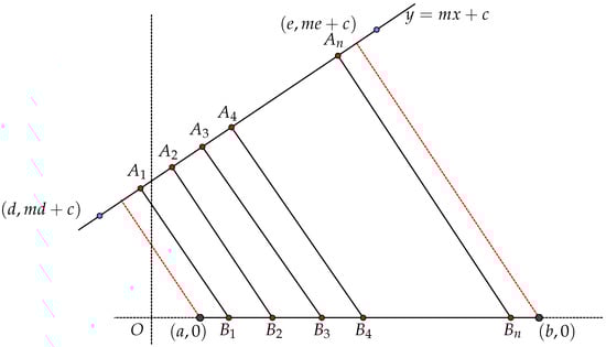
Let P be a Borel probability measure on ${\mathbb{R}}^2$ such that P is uniform on its support $\{(x,y)\in {\mathbb{R}}^2:a\le x\le b\mathrm{and}y=0\}$. For $n\in \mathbb{N}$ with $n\ge 2$, let ${\alpha }_n:=\{(a_i,m{a}_i+c):1\le i\le n\}$ be an optimal set of n-points for P so that the elements in the optimal sets lie on the line L between the two elements $(d,md+c)$ and $(e,me+c)$ (see Figure 1), where $d,e\in \mathbb{R}$ with $d<e$. Assume that

$$max\{a,(m^2+1)d+mc\}=aandmin\{b,(m^2+1)e+mc\}=b.$$

Then, $a_i={\displaystyle \frac{2i-1}{2n(1+m^2)}}(b-a)+{\displaystyle \frac{a-cm}{1+m^2}}$, for $1\le i\le n$, with the constrained quantization error

$$V_2={\displaystyle \frac{a^2\left(16m^2+1\right)+2ab\left(8m^2-1\right)+48acm+b^2\left(16m^2+1\right)+48bcm+48c^2}{48\left(m^2+1\right)}}.$$

For $n\ge 3$, we have

$$\begin{array}{cc}\hfill V_n=& {\displaystyle \frac{1}{12\left(m^2+1\right)n^3}}(-48{(a-b)}^2{m}^2+(a-b)(a-b+72cm+8(11a-2b)m^2)n\hfill \\ \hfill & -12(a-b)m(5c+(4a+b)m)n^2+12{(c+am)}^2{n}^3).\hfill \end{array}$$

Figure 1. Support of the probability distribution P is the closed interval joining the points $(a,0)$ and $(b,0)$; $A_i(a_i,m{a}_i+c)$ are the elements in an optimal set of n-points lying on the line $y=mx+c$ between the two points $(d,md+c)$ and $(e,me+c)$; and $B_i((m^2+1)a_i+mc,0)$ are the points where the perpendiculars through $A_i$ on the line $y=mx+c$ intersect the support of P.

Proof. 

For $n\ge 2$, let ${\alpha }_n:=\{(a_i,m{a}_i+c):1\le i\le n\}$ be an optimal set of n-points on L such that $d\le a_1<a_2<\cdots <a_{n-1}<a_n\le e$. Notice that the boundary of the Voronoi region of the element $(a_1,m{a}_1+c)$ intersects the support of P at the elements $(a,0)$ and $((m^2+1){\displaystyle \frac{(a_1+a_2)}{2}}+mc,0)$, and the boundary of the Voronoi region of $(a_n,m{a}_n+c)$ intersects the support of P at the elements $((m^2+1){\displaystyle \frac{(a_{n-1}+a_n)}{2}}+mc,0)$ and $(b,0)$. On the other hand, the boundaries of the Voronoi regions of $(a_i,m{a}_i+c)$ for $2\le i\le n-1$ intersect the support of P at the elements $((m^2+1){\displaystyle \frac{(a_{i-1}+a_i)}{2}}+mc,0)$ and $((m^2+1){\displaystyle \frac{(a_i+a_{i+1})}{2}}+mc,0)$. Since the Voronoi regions of the elements in an optimal set must have positive probability, we have

$$\begin{array}{cc}\hfill max\{a,(m^2+1)d+mc\}& \le (m^2+1)a_1+mc<(m^2+1)a_2+mc\hfill \\ \hfill & <\cdots <(m^2+1)a_n+mc\le min\{b,(m^2+1)e+mc\}.\hfill \end{array}$$

Let us consider the following two cases:

Case 1: $n=2$.

In this case, the distortion error due to the set ${\alpha }_2$ is given by

$$\begin{array}{cc}\hfill V(P;{\alpha }_2)=& {\int }_{\mathbb{R}}\underset{a\in {\alpha }_2}{min}{\parallel (x,0)-a\parallel }^{2}dP\left(x\right)\hfill \\ \hfill =& {\displaystyle \frac{1}{b-a}}({\int }_a^{(m^2+1){\displaystyle \frac{(a_1+a_2)}{2}}+mc}\rho ((x,0),(a_1,m{a}_1+c))dx\hfill \\ \hfill & +{\int }_{(m^2+1){\displaystyle \frac{(a_1+a_2)}{2}}+mc}^b\rho ((x,0),(a_2,m{a}_2+c))dx).\hfill \end{array}$$

Notice that $V(P;{\alpha }_2)$ is not always differentiable with respect to $a_1$ and $a_2$. By the hypothesis, we have

$$max\{a,(m^2+1)d+mc\}=a\mathrm{and}min\{b,(m^2+1)e+mc\}=b.$$

This guarantees that $V(P;{\alpha }_2)$ is differentiable with respect to $a_1$ and $a_2$.

Since ${\displaystyle \frac{\partial }{\partial a_1}}V(P;{\alpha }_2)=0$ and ${\displaystyle \frac{\partial }{\partial a_2}}V(P;{\alpha }_2)=0$, we can deduce that

$$-3a_1{m}^2+a_2{m}^2+2a-3a_1+a_2-2cm=0,\mathrm{and}$$

$$a_1{m}^2-3a_2{m}^2+a_1-3a_2+2b-2cm=0,$$

implying

$$a_1={\displaystyle \frac{1}{4(1+m^2)}}(b-a)+{\displaystyle \frac{a-cm}{1+m^2}}\mathrm{and}{a}_2={\displaystyle \frac{3}{4(1+m^2)}}(b-a)+{\displaystyle \frac{a-cm}{1+m^2}}$$

with the quantization error

$$V_2={\displaystyle \frac{a^2\left(16m^2+1\right)+2ab\left(8m^2-1\right)+48acm+b^2\left(16m^2+1\right)+48bcm+48c^2}{48\left(m^2+1\right)}}.$$

Case 2: $n\ge 3$.

In this case, the distortion error due to the set ${\alpha }_n$ is given by

$$\begin{array}{cc}\hfill V(P;{\alpha }_n)=& {\int }_{\mathbb{R}}\underset{a\in {\alpha }_n}{min}{\parallel (x,0)-a\parallel }^{2}dP\left(x\right)\hfill \\ \hfill =& {\displaystyle \frac{1}{b-a}}({\int }_a^{(m^2+1){\displaystyle \frac{(a_1+a_2)}{2}}+mc}\rho ((x,0),(a_1,m{a}_1+c))dx\hfill \\ \hfill & +\sum _{i=2}^{n-1}{\int }_{(m^2+1){\displaystyle \frac{(a_{i-1}+a_i)}{2}}+mc}^{(m^2+1){\displaystyle \frac{(a_i+a_{i+1})}{2}}+mc}\rho ((x,0),(a_i,m{a}_i+c))dx\hfill \\ \hfill & +{\int }_{(m^2+1){\displaystyle \frac{(a_{n-1}+a_n)}{2}}+mc}^b\rho ((x,0),(a_n,m{a}_n+c))dx).\hfill \end{array}$$

Since $V(P;{\alpha }_n)$ gives the optimal error and is always differentiable with respect to $a_i$ for $2\le i\le n-1$, we have ${\displaystyle \frac{\partial }{\partial a_i}}V(P;{\alpha }_n)=0$, yielding

$$a_{i+1}-a_i=a_i-a_{i-1}\mathrm{for}2\le i\le n-1$$

and implying

$$a_2-a_1=a_3-a_2=\cdots =a_n-a_{n-1}=k$$

(8)

for some real k. Due to the same reasoning as given in Case 1, we have ${\displaystyle \frac{\partial }{\partial a_1}}V(P;{\alpha }_n)=0$ and ${\displaystyle \frac{\partial }{\partial a_n}}V(P;{\alpha }_n)=0$, i.e.,

$$2(a-cm)-3a_1\left(m^2+1\right)+a_2\left(m^2+1\right)=0,\mathrm{and}$$

$$a_{n-1}\left(m^2+1\right)-3a_n\left(m^2+1\right)+2(b-cm)=0,$$

implying

$$a_1={\displaystyle \frac{a-cm}{1+m^2}}+{\displaystyle \frac{k}{2}}\mathrm{and}{a}_n={\displaystyle \frac{b-cm}{m^2+1}}-{\displaystyle \frac{k}{2}}.$$

(9)

Now, we have

$$\begin{array}{cc}\hfill b-a=& (a_1-a)+\sum _{i=2}^n(a_i-a_{i-1})+(b-a_n)=\left({\displaystyle \frac{a-cm}{1+m^2}}+{\displaystyle \frac{k}{2}}-a\right)+(n-1)k\hfill \\ \hfill & +\left(b-{\displaystyle \frac{b-cm}{1+m^2}}+{\displaystyle \frac{k}{2}}\right),\hfill \end{array}$$

which implies $k={\displaystyle \frac{b-a}{n(1+m^2)}}.$ Putting $k={\displaystyle \frac{b-a}{n(1+m^2)}}$, by the expressions given in (8) and (9), we can deduce that

$$a_i={\displaystyle \frac{2i-1}{2n(1+m^2)}}(b-a)+{\displaystyle \frac{a-cm}{1+m^2}}\mathrm{for}1\le i\le n.$$

To obtain the quantization error $V_n$, we proceed as follows.

Since the probability distribution P is uniform on its support, Equation (8) helps us to deduce that the distortion errors contributed by $a_2,a_3,\cdots ,a_{n-1}$, in their own Voronoi regions, are equal, i.e., each term in the sum

$$\sum _{i=2}^{n-1}{\int }_{(m^2+1){\displaystyle \frac{(a_{i-1}+a_i)}{2}}+mc}^{(m^2+1){\displaystyle \frac{(a_i+a_{i+1})}{2}}+mc}\rho ((x,0),(a_i,m{a}_i+c))dx$$

has the same value. Now, putting the values of $a_i$ for $2\le i\le n$ in terms of $a_1$ and k, we have

$$\begin{array}{cc}\hfill & V(P;{\alpha }_n)\hfill \\ \hfill =& {\int }_{\mathbb{R}}\underset{a\in {\alpha }_n}{min}{\parallel (x,0)-a\parallel }^{2}dP\left(x\right)\hfill \\ \hfill =& {\displaystyle \frac{1}{b-a}}({\int }_a^{(m^2+1){\displaystyle \frac{(2a_1+k)}{2}}+mc}\rho \left((x,0),(a_1,m{a}_1+c)\right)dx\hfill \\ \hfill & +(n-2){\int }_{(m^2+1){\displaystyle \frac{(2a_1+k)}{2}}+mc}^{(m^2+1){\displaystyle \frac{(2a_1+3k)}{2}}+mc}\rho \left((x,0),(a_1+k,m(a_1+k)+c)\right)dx\hfill \\ \hfill & +{\int }_{(m^2+1){\displaystyle \frac{(2a_1+k(2n-3))}{2}}+mc}^b\rho \left((x,0),(a_1+k(n-1),m(a_1+k(n-1))+c)\right)dx).\hfill \end{array}$$

Upon simplification, and putting $a_1={\displaystyle \frac{b-a}{2\left(m^2+1\right)n}}+{\displaystyle \frac{a-cm}{m^2+1}}$ and $k={\displaystyle \frac{b-a}{\left(m^2+1\right)n}}$ in the above expression, we have the quantization error as

$$\begin{array}{cc}\hfill V_n=& {\displaystyle \frac{1}{12\left(m^2+1\right)n^3}}(-48{(a-b)}^2{m}^2+(a-b)(a-b+72cm+8(11a-2b)m^2)n\hfill \\ \hfill & -12(a-b)m(5c+(4a+b)m)n^2+12{(c+am)}^2{n}^3).\hfill \end{array}$$

Thus, the proof of the theorem is complete. □

Remark 3.

In Theorem 1, the assumptions

$$max\{a,(m^2+1)d+mc\}=aandmin\{b,(m^2+1)e+mc\}=b$$

are necessary to guarantee that the elements in the optimal sets of n-points lie on the line segment joining the points $(d,md+c)$ and $(e,me+c)$. (For more details, please see Proposition 6.)

Let us now give the following corollary.

Corollary 3.

Let P be a Borel probability measure on ${\mathbb{R}}^2$ such that P is uniform on its support $\{(x,y)\in {\mathbb{R}}^2:0\le x\le 2\mathrm{and}y=0\}$. For $n\in \mathbb{N}$ with $n\ge 2$, let ${\alpha }_n$ be an optimal set of n-points for P such that the elements in the optimal set lie on the line $y=\sqrt{3}x$ between the elements $(0,0)$ and $(2,2\sqrt{3})$. Then,

$${\alpha }_n=\left\{\left({\displaystyle \frac{2i-1}{4n}},{\displaystyle \frac{2i-1}{4n}}\sqrt{3}\right):1\le i\le n\right\}and{V}_n=\left\{\begin{array}{cc}{\displaystyle \frac{49}{48}}& ifn=2,\\ {\displaystyle \frac{36n^2+49n-144}{12n^3}}& ifn\ge 3.\end{array}\right.$$

Proof. 

Putting $a=0,b=2,m=\sqrt{3},c=0,d=0,\mathrm{and}e=2$ in Theorem 1, we see that

$$max\{a,(m^2+1)d+mc\}=0=a\mathrm{and}min\{b,(m^2+1)e+mc\}=2=b.$$

Hence, by Theorem 1, we obtain the optimal sets ${\alpha }_n$ and the corresponding quantization errors $V_n$ as follows:

$${\alpha }_n=\left\{\left({\displaystyle \frac{2i-1}{4n}},{\displaystyle \frac{2i-1}{4n}}\sqrt{3}\right):1\le i\le n\right\}\mathrm{and}{V}_n=\left\{\begin{array}{cc}{\displaystyle \frac{49}{48}}& \mathrm{if}n=2,\\ {\displaystyle \frac{36n^2+49n-144}{12n^3}}& \mathrm{if}n\ge 3.\end{array}\right.$$

Thus, the proof of the corollary is complete. □

Remark 4.

If $m=0$, $c=0$, $d=a$, and $e=b$, then—by Theorem 1—the optimal set of n-points is given by ${\alpha }_n:=\{a+{\displaystyle \frac{2i-1}{2n}}(b-a):1\le i\le n\}$, and the corresponding quantization error is $V_n:=V_n\left(P\right)={\displaystyle \frac{{(a-b)}^2}{12n^2}},$ which is Theorem 2.1.1 in [26]. Thus, Theorem 1 generalizes Theorem 2.1.1 in [26].

The following proposition plays an important role in finding the optimal sets of n-points.

Proposition 6.

Let P be a Borel probability measure on ${\mathbb{R}}^2$ such that P is uniform on its support $\{(x,y)\in {\mathbb{R}}^2:a\le x\le b\mathrm{and}y=0\}$. For $n\in \mathbb{N}$ with $n\ge 2$, let ${\alpha }_n:=\{(a_i,m{a}_i+c):1\le i\le n\}$ be an optimal set of n-points for P so that the elements in the optimal set lie on the line L between the two elements $(d,md+c)$ and $(e,me+c)$, where $d,e\in \mathbb{R}$ with $d<e$. Then, $\left(i\right)$ if $(m^2+1)d+mc>a$ (or $(m^2+1)e+mc<b$), let N be the largest positive integer such that

$$d<{\displaystyle \frac{1}{2N(1+m^2)}}(b-a)+{\displaystyle \frac{a-cm}{1+m^2}}\left(or{\displaystyle \frac{2N-1}{2N(1+m^2)}}(b-a)+{\displaystyle \frac{a-cm}{1+m^2}}<e\right).$$

Then, for all $n\ge N+1$, the optimal sets ${\alpha }_n$ always contain the end element $(d,md+c)$ (or $(e,me+c))$. On the other hand, $\left(ii\right)$ if $(m^2+1)d+mc>a$ and $(m^2+1)e+mc<b$, let $N:=max\{N_1,N_2\}$, where $N_1$ and $N_2$ are the largest positive integers such that

$$d<{\displaystyle \frac{1}{2N_1(1+m^2)}}(b-a)+{\displaystyle \frac{a-cm}{1+m^2}}\mathrm{and}{\displaystyle \frac{2N_2-1}{2N_2(1+m^2)}}(b-a)+{\displaystyle \frac{a-cm}{1+m^2}}<e.$$

Then, for all $n\ge N+1$, the optimal sets ${\alpha }_n$ always contain the end elements $(d,md+c)$ and $(e,me+c)$.

Proof. 

Let ${\alpha }_n:=\{(a_i,m{a}_i+c):1\le i\le n\}$ be an optimal set of n-points for P so that the elements in the optimal set lie on the line L between the two elements $(d,md+c)$ and $(e,me+c)$, where $d,e\in \mathbb{R}$ with $d<e$. Also, notice that the perpendiculars on the line L passing through the elements $(a_i,m{a}_i+c)$ intersect the support of P at the elements $((m^2+1)a_i+mc,0)$, respectively, where $1\le i\le n$. By Theorem 1, we know that

$$a_i={\displaystyle \frac{2i-1}{2n(1+m^2)}}(b-a)+{\displaystyle \frac{a-cm}{1+m^2}}\mathrm{for}1\le i\le n.$$

Suppose that $(m^2+1)d+mc>a$. Let $n=N$ be the largest positive integer such that

$$\begin{array}{cc}\hfill & (m^2+1)d+mc<(m^2+1)a_1+mc,\mathrm{i}.\mathrm{e}.,\hfill \\ \hfill & d<a_1,\mathrm{i}.\mathrm{e}.,d<{\displaystyle \frac{1}{2N(1+m^2)}}(b-a)+{\displaystyle \frac{a-cm}{1+m^2}}.\hfill \end{array}$$

(10)

Notice that the sequence $\{{\displaystyle \frac{1}{2n(1+m^2)}}(b-a)+{\displaystyle \frac{a-cm}{1+m^2}}\}$ is strictly decreasing. Hence, for all $n\ge N+1$, the optimal sets ${\alpha }_n$ always contain the end element $(d,md+c)$. Suppose that $(m^2+1)e+mc<b$. Let $n=N$ be the largest positive integer such that

$$\begin{array}{cc}\hfill & (m^2+1)a_N+mc<(m^2+1)e+mc,\mathrm{i}.\mathrm{e}.,a_N<e,\mathrm{i}.\mathrm{e}.,\hfill \\ \hfill & {\displaystyle \frac{2N-1}{2N(1+m^2)}}(b-a)+{\displaystyle \frac{a-cm}{1+m^2}}<e.\hfill \end{array}$$

(11)

Notice that the sequence $\{{\displaystyle \frac{2n-1}{2n(1+m^2)}}(b-a)+{\displaystyle \frac{a-cm}{1+m^2}}\}$ is strictly increasing. Hence, for all $n\ge N+1$, the optimal sets ${\alpha }_n$ always contain the end element $(e,me+c)$. Next, suppose that $(m^2+1)d+mc>a$ and $(m^2+1)e+mc<b$. Choose $N_1$ and $N_2$ to be the same as N described in (10) and (11), respectively. Let $N=max\{N_1,N_2\}$. Then, for all $n\ge N+1$, the optimal sets ${\alpha }_n$ always contain the end elements $(d,md+c)$ and $(e,me+c)$. Thus, the proof of the proposition is complete. □

Note 1.

In the following, we state and prove two theorems: Theorems 2 and 3. To facilitate the proofs in both the theorems, Proposition 6 can be used. However, in the proof of Theorem 2, we do not use Proposition 6; on the other hand, in the proof of Theorem 3, we use Proposition 6.

Theorem 2.

Let P be a Borel probability measure on ${\mathbb{R}}^2$ such that P is uniform on its support $\{(x,y)\in {\mathbb{R}}^2:0\le x\le 2\mathrm{and}y=0\}$. For $n\in \mathbb{N}$, let ${\alpha }_n:=\{(a_i,1):1\le i\le n\}$ be an optimal set of n-points for P so that the elements in the optimal sets lie on the line $y=1$ between the two elements $({\displaystyle \frac{1}{2}},1)$ and $({\displaystyle \frac{3}{2}},1)$. Then, ${\alpha }_1=\left\{(1,1)\right\}$, ${\alpha }_2=\{({\displaystyle \frac{1}{2}},1),({\displaystyle \frac{3}{2}},1)\}$, and for $n\ge 3$, we have

$$a_i=\left\{\begin{array}{cc}{\displaystyle \frac{1}{2}}& ifi=1,\\ {\displaystyle \frac{1}{2}}+{\displaystyle \frac{(i-1)}{(n-1)}}& if2\le i\le n-1,\\ {\displaystyle \frac{3}{2}}& ifi=n.\end{array}\right.$$

Additionally, the quantization error for n-points is given by $V_n={\displaystyle \frac{25n^2-50n+26}{24{(n-1)}^2}}$.

Proof. 

The proofs of ${\alpha }_1=\left\{(1,1)\right\}$ and ${\alpha }_2=\{({\displaystyle \frac{1}{2}},1),({\displaystyle \frac{3}{2}},1)\}$ are routine. We will now give the proof for $n\ge 3$. Let ${\alpha }_n:=\{(t,1):t=a_i\mathrm{for}1\le i\le n\}$ be an optimal set of n-points such that ${\displaystyle \frac{1}{2}}\le a_1<a_2<\cdots <a_{n-1}<a_n\le {\displaystyle \frac{3}{2}}$. Notice that the boundary of the Voronoi region of the element $(a_1,1)$ intersects the support of P at the elements $(0,0)$ and $({\displaystyle \frac{1}{2}}(a_1+a_2),0)$, and the boundary of the Voronoi region of $(a_n,1)$ intersects the support of P at the elements $({\displaystyle \frac{1}{2}}(a_{n-1}+a_n),0)$ and $(2,0)$. On the other hand, the boundaries of the Voronoi regions of $(a_i,1)$ for $2\le i\le n-1$ intersect the support of P at the elements $({\displaystyle \frac{1}{2}}(a_{i-1}+a_i),0)$ and $({\displaystyle \frac{1}{2}}(a_i+a_{i+1}),0)$. Thus, the distortion error due to the set ${\alpha }_n$ is given by

$$\begin{array}{cc}\hfill & V(P;{\alpha }_n)={\int }_{\mathbb{R}}\underset{a\in {\alpha }_n}{min}{\parallel (x,0)-a\parallel }^{2}dP\left(x\right)\hfill \\ \hfill & ={\int }_0^{{\displaystyle \frac{1}{2}}\left(a_1+a_2\right)}{\displaystyle \frac{1}{2}}\left({\left(x-a_1\right)}^2+1\right)dx+\sum _{i=2}^{n-1}{\int }_{{\displaystyle \frac{1}{2}}\left(a_{i-1}+a_i\right)}^{{\displaystyle \frac{1}{2}}\left(a_{i+1}+a_i\right)}{\displaystyle \frac{1}{2}}\left({\left(x-a_i\right)}^2+1\right)dx\hfill \\ \hfill & +{\int }_{{\displaystyle \frac{1}{2}}\left(a_{n-1}+a_n\right)}^2{\displaystyle \frac{1}{2}}\left({\left(x-a_n\right)}^2+1\right)dx.\hfill \end{array}$$

Since $V(P;{\alpha }_n)$ gives the optimal error and is differentiable with respect to $a_i$ for $2\le i\le n-1$, we have ${\displaystyle \frac{\partial }{\partial a_i}}V(P;{\alpha }_n)=0$, implying

$$a_{i+1}-a_i=a_i-a_{i-1}\mathrm{for}2\le i\le n-1.$$

This yields the fact that

$$a_2-a_1=a_3-a_2=\cdots =a_n-a_{n-1}=k$$

(12)

for some real number $0<k<1$. By the equations in $\left(12\right)$, we see that all terms in the sum ${\sum }_{i=2}^{n-1}{\int }_{{\displaystyle \frac{1}{2}}\left(a_{i-1}+a_i\right)}^{{\displaystyle \frac{1}{2}}\left(a_{i+1}+a_i\right)}{\displaystyle \frac{1}{2}}\left({\left(x-a_i\right)}^2+1\right)dx$ have the same value. Again, by the equations in (12), we have

$$a_2=k+a_1,a_3=2k+a_1,\cdots ,a_n=(n-1)k+a_1.$$

Hence,

$$\begin{array}{cc}\hfill V(P;{\alpha }_n)& ={\int }_0^{{\displaystyle \frac{1}{2}}\left(2a_1+k\right)}{\displaystyle \frac{1}{2}}\left({\left(x-a_1\right)}^2+1\right)dx\hfill \\ \hfill & +(n-2){\int }_{{\displaystyle \frac{1}{2}}\left(2a_1+k\right)}^{{\displaystyle \frac{1}{2}}\left(2a_1+3k\right)}{\displaystyle \frac{1}{2}}\left({\left(x-\left(a_1+k\right)\right)}^2+1\right)dx\hfill \\ \hfill & +{\int }_{{\displaystyle \frac{1}{2}}\left(2a_1+k(2n-3)\right)}^2{\displaystyle \frac{1}{2}}\left({\left(x-\left(a_1+k(n-1)\right)\right)}^2+1\right)dx,\hfill \end{array}$$

which, upon simplification, yields

$$\begin{array}{cc}\hfill V(P;{\alpha }_n)& ={\displaystyle \frac{1}{24}}(-12a_1(k(n-1)-2)\left(a_1+k(n-1)-2\right)\hfill \\ \hfill & -k(n-1)\left(4k^2{n}^2-8k(k+3)n+3{(k+4)}^2\right)+56),\hfill \end{array}$$

which is minimum if $a_1={\displaystyle \frac{1}{2}}$ and $k={\displaystyle \frac{1}{n-1}}$, where the minimum value is ${\displaystyle \frac{25n^2-50n+26}{24{(n-1)}^2}}$. As $k={\displaystyle \frac{1}{n-1}}$ and $a_1={\displaystyle \frac{1}{2}}$, using the expression (12), we obtain

$$a_i=\left\{\begin{array}{cc}{\displaystyle \frac{1}{2}}& \mathrm{if}i=1,\\ {\displaystyle \frac{1}{2}}+{\displaystyle \frac{(i-1)}{(n-1)}}& \mathrm{if}2\le i\le n-1,\\ {\displaystyle \frac{3}{2}}& \mathrm{if}i=n,\end{array}\right.$$

with the quantization error $V_n={\displaystyle \frac{25n^2-50n+26}{24{(n-1)}^2}}$. Thus, the proof of the theorem is complete. □

Remark 5.

Comparing Theorem 2 with Proposition 6, we have $a=0,b=2,m=0,c=1,d={\displaystyle \frac{1}{2}},$ and $e={\displaystyle \frac{3}{2}}$. As such,

$$(m^2+1)d+mc={\displaystyle \frac{1}{2}}>aand(m^2+1)e+mc={\displaystyle \frac{3}{2}}<b.$$

Let $n=N_1$ be the largest positive integer such that

$$d<{\displaystyle \frac{1}{2N_1(1+m^2)}}(b-a)+{\displaystyle \frac{a-cm}{1+m^2}},$$

which is true if $N_1<2$, i.e., $N_1=1$. Let $n=N_2$ be the largest positive integer such that

$${\displaystyle \frac{2N_2-1}{2N_2(1+m^2)}}(b-a)+{\displaystyle \frac{a-cm}{1+m^2}}<e,$$

which is true if $N_2<2$, i.e., $N_2=1$. Take $N=max\{N_1,N_2\}$. Then, $N=1$. By Proposition 6, we can conclude that, for all $n\ge 2$, the optimal sets ${\alpha }_n$ will contain the end elements $({\displaystyle \frac{1}{2}},1)$ and $({\displaystyle \frac{3}{2}},1)$, which is clearly true by Theorem 2.

Theorem 3.

Let P be a Borel probability measure on ${\mathbb{R}}^2$ such that P is uniform on its support $\{(x,y)\in {\mathbb{R}}^2:0\le x\le 2\mathrm{and}y=0\}$. For $n\in \mathbb{N}$, let ${\alpha }_n:=\{(a_i,1):1\le i\le n\}$ be an optimal set of n-points for P so that the elements in the optimal set lie on the line $y=1$ between the two elements $(0,1)$ and $({\displaystyle \frac{28}{15}},1)$, i.e., $0\le a_1<a_2<\cdots <a_n\le {\displaystyle \frac{28}{15}}$. Then, ${\alpha }_1=\left\{(1,1)\right\}$, and for $1\le n\le 7$, we have

$${\alpha }_n=\left\{\left({\displaystyle \frac{2i-1}{n}},1\right):1\le i\le n\right\}.$$

On the other hand, for $n\ge 8$, we obtain

$$a_i=\left\{\begin{array}{cc}{\displaystyle \frac{28(2i-1)}{15(2n-1)}}& \mathit{if}1\le i\le n-1,\\ {\displaystyle \frac{28}{15}}& \mathit{if}i=n,\end{array}\right.$$

and the quantization error for n-points is given by $V_n={\displaystyle \frac{7\left(5788\right(n-1)n+3015)}{10125{(1-2n)}^2}}$.

Proof. 

Let ${\alpha }_n:=\{(t,1):t=a_i\mathrm{for}1\le i\le n\}$ be an optimal set of n-points such that $0\le a_1<a_2<\cdots <a_{n-1}<a_n\le {\displaystyle \frac{28}{15}}$ for all $n\in \mathbb{N}$. Using Proposition 6, it can be proved that, for all $n\ge 8$, the optimal sets always contain the end element ${\displaystyle \frac{28}{15}}$, i.e., $a_n={\displaystyle \frac{28}{15}}$, for all $n\ge 8$. The proofs of ${\alpha }_1=\left\{(1,1)\right\}$, and for $1\le n\le 7$, are

$${\alpha }_n=\left\{\left({\displaystyle \frac{2i-1}{n}},1\right):1\le i\le n\right\},$$

which are routine. Here, we prove the optimal sets of n-points for all $n\ge 8$. Proceeding in the similar lines as given in the proof of Theorem 2, we have

$$a_2-a_1=a_3-a_2=\cdots =a_n-a_{n-1}=k$$

for some real k, which implies

$$a_1=a_n-(n-1)k,a_2=a_n-(n-2)k,\cdots ,a_{n-1}=a_n-k.$$

Also, by using ${\displaystyle \frac{\partial }{\partial a_1}}V(P;{\alpha }_n)=0$, we get $3a_1-a_2=0$, which implies that $a_1={\displaystyle \frac{k}{2}}$. Now, we have

$${\displaystyle \frac{k}{2}}=a_1=a_n-(n-1)k={\displaystyle \frac{28}{15}}-(n-1)k,$$

and this yields $k={\displaystyle \frac{56}{15(2n-1)}}$. Using $a_n={\displaystyle \frac{28}{15}}$ and $k={\displaystyle \frac{56}{15(2n-1)}}$, we get $a_i={\displaystyle \frac{28(2i-1)}{15(2n-1)}}$ for $1\le i\le n-1$ with the quantization error

$$\begin{array}{cc}\hfill V(P;{\alpha }_n)=& {\displaystyle \frac{1}{2}}\left({\int }_0^{{\displaystyle \frac{1}{2}}\left(2a_n-k(2n-3)\right)}\left({\left(x-\left(a_n-k(n-1)\right)\right)}^2+1\right)dx\right.\hfill \\ \hfill & +(n-2){\int }_{{\displaystyle \frac{1}{2}}\left(2a_n-3k\right)}^{{\displaystyle \frac{1}{2}}\left(2a_n-k\right)}\left({\left(x-\left(a_n-k\right)\right)}^2+1\right)dx\hfill \\ \hfill & \left.+{\int }_{{\displaystyle \frac{1}{2}}\left(2a_n-k\right)}^2\left({\left(x-a_n\right)}^2+1\right)dx\right)\hfill \\ \hfill =& {\displaystyle \frac{1}{24}}(12k^2{n}^2{a}_n-24k^{2}n{a}_n+12k^2{a}_n-12kn{a}_n^2+12k{a}_n^2+24a_n^2\hfill \\ \hfill & -48a_n-4k^3{n}^3+12k^3{n}^2-11k^{3}n+3k^3+56)\hfill \\ \hfill =& {\displaystyle \frac{7\left(5788\right(n-1)n+3015)}{10125{(1-2n)}^2}}.\hfill \end{array}$$

This completes the proof. □

4. Constrained Quantization When the Support Lies on a Circle and the Optimal Elements Lie on Another Circle

Let $O(0,0)$ be the origin of the Cartesian plane. Let C be the unit circle given by the following parametric equations:

$$C:=\left\{\right(x,y):x=cost,y=sint\mathrm{for}0\le t\le 2\pi \}.$$

Let the positive direction of the x-axis cut the circle at the element $A_0$, i.e., $A_0$ is represented by the parametric value $t=0$. Let s be the distance of an element on C along the arc starting from the element $A_0$ in the counterclockwise direction. Then,

$$ds=\sqrt{{\left({\displaystyle \frac{dx}{dt}}\right)}^2+{\left({\displaystyle \frac{dy}{dt}}\right)}^2}dt=dt.$$

Let P be a uniform distribution with support the unit circle C. Then, the probability density function $f(x,y)$ for P is given by

$$f(x,y)=\left\{\begin{array}{cc}{\displaystyle \frac{1}{2\pi }}& \mathrm{if}(x,y)\in C,\\ 0& \mathrm{otherwise}.\end{array}\right.$$

Thus, we have $dP\left(s\right)=P\left(ds\right)=f(x,y)ds={\displaystyle \frac{1}{2\pi }}dt$. Moreover, we parameterize points on the unit circle by the central angle $t\in [0,2\pi )$. This allows us to express distances and arc-based quantities in terms of angular separation, which will be used in the estimates that follow.

Let L be a concentric circle with C, and L has radius a, i.e., the parametric representation of the circle L is given by

$$L:=\left\{\right(x,y):x=acos\theta ,y=asin\theta \mathrm{for}0\le \theta \le 2\pi \}.$$

In this section, we determine the optimal sets of n-points and the nth constrained quantization errors for the uniform distribution P on C under the condition that the elements in an optimal set lie on the circle L. Let the line $O{A}_0$ cut the circle L at the element $B_0$, i.e., $B_0$ is represented on the circle L by the parameter $\theta =0$.

Proposition 7.

Any element on the circle L forms an optimal set of one-point with the quantization error $V_1=1+a^2.$

Proof. 

Let $\alpha :=\left\{\right(acos\theta ,asin\theta \left)\right\}$, where $0\le \theta \le 2\pi$, form an optimal set of one-point. Then, the distortion error $V(P;\alpha )$ is given by

$$V(P;\alpha )={\int }_C{\displaystyle \frac{1}{2\pi }}\rho ((cost,sint),(acos\theta ,asin\theta ))dt=1+a^2,$$

which does not depend on $\theta$ for any $0\le \theta \le 2\pi$. Hence, any element on the circle L forms an optimal set of one-point, and the quantization error for one-point is given by $V_1=1+a^2$. □

Proposition 8.

A set of the form $\left\{\right(acos\theta ,asin\theta ),(-acos\theta ,-asin\theta \left)\right\}$, where $0\le \theta \le 2\pi$, forms an optimal set of two-points with the quantization error $V_2=1+a^2-{\displaystyle \frac{4a}{\pi }}$.

Proof. 

Let $\alpha :=\{(acos{\theta }_1,asin{\theta }_1),(acos{\theta }_2,asin{\theta }_2)\}$, where $0\le {\theta }_1<{\theta }_2\le 2\pi$, form an optimal set of two-points. Notice that the boundary of the Voronoi regions of the two elements in the optimal set is the line joining the two points given by the parameters $\theta ={\displaystyle \frac{{\theta }_1+{\theta }_2}{2}}$ and $\theta =\pi +{\displaystyle \frac{{\theta }_1+{\theta }_2}{2}}$. Then, the distortion error is given by

$$\begin{array}{cc}\hfill V(P;\alpha )=& {\displaystyle \frac{1}{2\pi }}({\int }_{-\pi +{\displaystyle \frac{{\theta }_1+{\theta }_2}{2}}}^{{\displaystyle \frac{{\theta }_1+{\theta }_2}{2}}}\rho \left((cost,sint),(acos{\theta }_1,asin{\theta }_1)\right)dt\hfill \\ \hfill & +{\int }_{{\displaystyle \frac{{\theta }_1+{\theta }_2}{2}}}^{\pi +{\displaystyle \frac{{\theta }_1+{\theta }_2}{2}}}\rho \left((cost,sint),(acos{\theta }_2,asin{\theta }_2)\right)dt)\hfill \\ \hfill =& {\displaystyle \frac{1}{2\pi }}({\int }_{-\pi +{\displaystyle \frac{{\theta }_1+{\theta }_2}{2}}}^{{\displaystyle \frac{{\theta }_1+{\theta }_2}{2}}}\left(1+a^2-2acos(t-{\theta }_1)\right)dt\hfill \\ \hfill & +{\int }_{{\displaystyle \frac{{\theta }_1+{\theta }_2}{2}}}^{\pi +{\displaystyle \frac{{\theta }_1+{\theta }_2}{2}}}\left(1+a^2-2acos(\theta -{\theta }_2)\right)dt),\hfill \end{array}$$

which, upon simplification, yields that

$$V(P;\alpha )={\displaystyle \frac{1}{2\pi }}\left((1+a^2)2\pi -8asin{\displaystyle \frac{{\theta }_2-{\theta }_1}{2}}\right).$$

Since $0<{\displaystyle \frac{{\theta }_2-{\theta }_1}{2}}<\pi$, we can say that $V(P;\alpha )$ is minimum if ${\theta }_2-{\theta }_1=\pi$. Thus, an optimal set of two-points is given by $\left\{\right(acos\theta ,asin\theta ),(-acos\theta ,-asin\theta \left)\right\}$ for $0\le \theta \le 2\pi$ with the constrained quantization error $V_2=1+a^2-{\displaystyle \frac{4a}{\pi }}$, which yields the proposition. □

Theorem 4.

Let ${\alpha }_n$ be an optimal set of n-points for the uniform distribution P on the unit circle C for $n\in \mathbb{N}$ with $n\ge 3$. Then,

$${\alpha }_n=\left\{\left(acos{\displaystyle \frac{(2i-1)\pi }{n}},asin{\displaystyle \frac{(2i-1)\pi }{n}}\right):i=1,2,\cdots ,n\right\}$$

and the corresponding quantization error is given by $V_n=a^2+1-{\displaystyle \frac{2an}{\pi }}sin{\displaystyle \frac{\pi }{n}}.$

Proof. 

Let ${\alpha }_n:=\{a_1,a_2,\cdots ,a_n\}$ be an optimal set of n-points for P with $n\ge 3$ such that the elements in the optimal set lie on the circle L. Let the boundary of the Voronoi regions of $a_i$ cut the circle L, as well as, in fact, the circle C, at the elements given by the parameters ${\theta }_{i-1}$ and ${\theta }_i$, where $1\le i\le n$. Since the circles have rotational symmetry, without any loss of generality, we can assume that ${\theta }_0=0$ and ${\theta }_n=2\pi$. Then, each $a_i$ on L has the parametric representation ${\displaystyle \frac{1}{2}}({\theta }_{i-1}+{\theta }_i)$ for $1\le i\le n$. Then, the quantization error for n-points is given by

$$\begin{array}{cc}\hfill V(P;{\alpha }_n)& ={\int }_C\underset{u\in {\alpha }_n}{min}\rho ((cost,sint),u)dP\left(s\right)\hfill \\ \hfill & =\sum _{i=1}^n{\int }_{{\theta }_{i-1}}^{{\theta }_i}{\displaystyle \frac{1}{2\pi }}\rho \left(((cost,sint),({\displaystyle \frac{1}{2}}cos{\displaystyle \frac{{\theta }_{i-1}+{\theta }_i}{2}},{\displaystyle \frac{1}{2}}sin{\displaystyle \frac{{\theta }_{i-1}+{\theta }_i}{2}}))\right)dt\hfill \\ \hfill & =\sum _{i=1}^n{\int }_{{\theta }_{i-1}}^{{\theta }_i}{\displaystyle \frac{1}{2\pi }}\left(a^2-2acos(-{\displaystyle \frac{{\theta }_{i-1}}{2}}-{\displaystyle \frac{{\theta }_i}{2}}+t)+1\right)d\theta \hfill \\ \hfill & =\sum _{i=1}^n{\displaystyle \frac{1}{2\pi }}\left((a^2+1)({\theta }_i-{\theta }_{i-1})-4asin{\displaystyle \frac{{\theta }_i-{\theta }_{i-1}}{2}}\right),\hfill \end{array}$$

upon simplification, which yields

$$V(P;{\alpha }_n)=a^2+1-{\displaystyle \frac{2a}{\pi }}\sum _{i=1}^{n}sin{\displaystyle \frac{{\theta }_i-{\theta }_{i-1}}{2}}.$$

(13)

Since $V(P;{\alpha }_n)$ gives the optimal error and is differentiable with respect to ${\theta }_i$ for all $1\le i\le n-1$, we have ${\displaystyle \frac{\partial }{\partial {\theta }_i}}V(P;\alpha )=0$. For $1\le i\le n-1$, the equations ${\displaystyle \frac{\partial }{\partial {\theta }_i}}V(P;\alpha )=0$ imply that

$$cos{\displaystyle \frac{{\theta }_i-{\theta }_{i-1}}{2}}=cos{\displaystyle \frac{{\theta }_{i+1}-{\theta }_i}{2}}\mathrm{yielding}$$

$${\displaystyle \frac{{\theta }_i-{\theta }_{i-1}}{2}}={\displaystyle \frac{{\theta }_{i+1}-{\theta }_i}{2}},\mathrm{or}{\displaystyle \frac{{\theta }_i-{\theta }_{i-1}}{2}}=2\pi -{\displaystyle \frac{{\theta }_{i+1}-{\theta }_i}{2}}.$$

Without any loss of generality, for $1\le i\le n-1$, we can take ${\displaystyle \frac{{\theta }_i-{\theta }_{i-1}}{2}}={\displaystyle \frac{{\theta }_{i+1}-{\theta }_i}{2}}$. This yields the fact that

$${\theta }_1-{\theta }_0={\theta }_2-{\theta }_1={\theta }_3-{\theta }_2=\cdots ={\theta }_n-{\theta }_{n-1}={\displaystyle \frac{2\pi }{n}}.$$

Thus, we have ${\theta }_i={\displaystyle \frac{2\pi i}{n}}$ for $i=1,2,\cdots ,n$. Hence, if ${\alpha }_n:=\{a_1,a_2,\cdots ,a_n\}$ is an optimal set of n-points, then

$$a_i=\left(acos{\displaystyle \frac{(2i-1)\pi }{n}},asin{\displaystyle \frac{(2i-1)\pi }{n}}\right)\mathrm{for}i=1,2,\cdots ,n,$$

and the quantization error for n-points, by (13), is given by

$$\begin{array}{c}\hfill V_n=V(P;{\alpha }_n)=a^2+1-{\displaystyle \frac{2an}{\pi }}sin{\displaystyle \frac{\pi }{n}}.\end{array}$$

Thus, the proof of the theorem is complete. □

5. Constrained Quantization When the Support Lies on a Chord of a Circle and the Optimal Elements Lie on the Circle

Let C be a circle with center $(0,0)$ and radius one, i.e., the equation of the circle is $x^2+y^2=1,$ whose parametric representations are $x=cos\theta$ and $y=sin\theta$, where $0\le \theta \le 2\pi$. Thus, if $(cos\theta ,sin\theta )$ is an element on the circle, then we will represent it by $\theta$. Let P be a Borel probability measure on ${\mathbb{R}}^2$ such that P has support a chord of the circle and where P is uniform on its support. We now investigate the optimal sets of n-points and the nth constrained quantization errors for all $n\in \mathbb{N}$ so that the optimal elements lie on the circle. The two cases can happen as described in the following two subsections.

5.1. Chord Is a Diameter of the Circle

Without any loss of generality, let us consider the horizontal diameter as the support of P, i.e., the support of P is the closed interval $\left\{\right(x,y):-1\le x\le 1,y=0\}$. Then, the probability density function is given by

$$f(x,y)=\left\{\begin{array}{cc}{\displaystyle \frac{1}{2}}& \mathrm{if}-1\le x\le 1\mathrm{and}y=0,\\ 0& \mathrm{otherwise}.\end{array}\right.$$

Recall Fact 1. Here, we have $dP\left(s\right)=P\left(ds\right)=P\left(dx\right)=dP\left(x\right)=f(x,0)dx$. Let ${\alpha }_n$ be an optimal set of n-points for any $n\ge 1$. We know that an optimal set of one-point always exists. For any $n\ge 2$, since the boundary of the Voronoi regions of any two optimal elements (in this case) passes through the center of the circle—from the geometry—we can see that, among n Voronoi regions, only two Voronoi regions contain elements from the support of P, i.e., only two Voronoi regions have positive probability. Hence, the optimal sets of n-points exist only for $n=1$ and $n=2$, and they do not exist for any $n\ge 3$.

We now calculate the optimal sets of one-point and the two-points in the following propositions.

Proposition 9.

Any element on the circle forms an optimal set of one-point with the constrained quantization error $V_1={\displaystyle \frac{4}{3}}$.

Proof. 

Let $(cos\theta ,sin\theta )$ be an element on the circle. Then, the distortion error for P with respect to this element is given by

$$\begin{array}{cc}\hfill V(P;\{(cos\theta ,sin\theta )\left\}\right)=& {\int }_{-1}^1\rho ((x,0),(cos\theta ,sin\theta ))dP\left(x\right)\hfill \\ \hfill =& {\displaystyle \frac{1}{2}}{\int }_{-1}^1\rho ((x,0),(cos\theta ,sin\theta ))dx={\displaystyle \frac{4}{3}},\hfill \end{array}$$

which does not depend on $\theta$. Hence, any element on the circle forms an optimal set of one-point with the constrained quantization error $V_1={\displaystyle \frac{4}{3}}$. □

Proposition 10.

The set $\left\{\right(-1,0),(1,0\left)\right\}$ forms an optimal set of two-points with the constrained quantization error $V_2={\displaystyle \frac{1}{3}}$.

Proof. 

From the geometry, we can see that the boundary of any two elements on the circle passes through the center of the circle. Thus, in an optimal set of two-points, one Voronoi region will contain the left half, and the other Voronoi region will contain the right half of the support of P. Hence, by the routine calculation, we can show that $\left\{\right(-1,0),(1,0\left)\right\}$ forms an optimal set of two-points with the constrained quantization error

$$V_2={\displaystyle \frac{1}{2}}\left({\int }_{-1}^0\rho ((x,0),(-1,0))dx+{\int }_0^1\rho ((x,0),(1,0))dx\right)={\displaystyle \frac{1}{3}}.$$

Thus, the proof of the proposition is complete. □

5.2. Chord Is Not a Diameter of the Circle

In this case, for definiteness sake, we investigate the optimal sets of n-points and the nth constrained quantization errors for a Borel probability measure P on ${\mathbb{R}}^2$ such that P has support the chord $y=-{\displaystyle \frac{1}{2}}$ for $-{\displaystyle \frac{\sqrt{3}}{2}}\le x\le {\displaystyle \frac{\sqrt{3}}{2}}$, where P is uniform. Then, the probability density function for P is given by

$$f(x,y)=\left\{\begin{array}{cc}{\displaystyle \frac{1}{\sqrt{3}}}& \mathrm{if}-{\displaystyle \frac{\sqrt{3}}{2}}\le x\le {\displaystyle \frac{\sqrt{3}}{2}}\mathrm{and}y=-{\displaystyle \frac{1}{2}},\\ 0& \mathrm{otherwise}.\end{array}\right.$$

Recall that the circle has rotational symmetry. Thus, for any other chord, the technique of finding the optimal sets of n-points and the nth constrained quantization errors will be similar. Here, we have $dP\left(s\right)=P\left(ds\right)=P\left(dx\right)=dP\left(x\right)=f(x,-{\displaystyle \frac{1}{2}})dx$, where x varies over the line $y=-{\displaystyle \frac{1}{2}}$. The arc of the circle subtended by the chord is represented by $\theta$ for ${\displaystyle \frac{7\pi }{6}}\le \theta \le {\displaystyle \frac{11\pi }{6}}$. Moreover, the circle is geometrically symmetric with respect to the line $y=0$, and also the probability measure is symmetric with respect to the line $y=0$, i.e., if two intervals of the same length lie on the support of P and are equidistant from the line $y=0$, then they have the same probability. In proving the results, we can use this symmetry of the circle.

Proposition 11.

The set $\left\{\right(0,-1\left)\right\}$ forms an optimal set of one-point with the quantization error $V_1={\displaystyle \frac{1}{2}}$.

Proof. 

Let us consider an element $(cos\theta ,sin\theta )$ on the circle. The distortion error for P with respect to the set $\left\{\right(cos\theta ,sin\theta \left)\right\}$ is given by

$$V(P;\left\{(cos\theta ,sin\theta )\right\})={\int }_{-{\displaystyle \frac{\sqrt{3}}{2}}}^{{\displaystyle \frac{\sqrt{3}}{2}}}{\displaystyle \frac{1}{\sqrt{3}}}\rho ((x,-{\displaystyle \frac{1}{2}}),(cos\theta ,sin\theta ))dx=sin\theta +{\displaystyle \frac{3}{2}},$$

the minimum value of which is ${\displaystyle \frac{1}{2}}$ and occurs when $\theta ={\displaystyle \frac{3\pi }{2}}$ (see Figure 2). Thus, the proof of the proposition is yielded. □

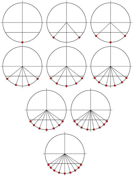
Figure 2. The optimal configuration of n elements for $1\le n\le 9$.

Proposition 12.

The optimal set of two-points is given by

$$\left\{2\pi -2{tan}^{-1}\left({\displaystyle \frac{\sqrt{3}}{2}}+{\displaystyle \frac{\sqrt{7}}{2}}\right),\pi +2{tan}^{-1}\left({\displaystyle \frac{\sqrt{3}}{2}}+{\displaystyle \frac{\sqrt{7}}{2}}\right)\right\}$$

with the quantization error $V_2={\displaystyle \frac{1}{2}}\left(3-\sqrt{7}\right)$.

Proof. 

Since the probability measure is symmetric with respect to the line $y=0$, we can assume that, in an optimal set of two-points, the Voronoi region of one element will contain the left half of the chord and the Voronoi region of the other element will contain the right half of the chord, i.e., the boundary of the two Voronoi regions is the y-axis. Let the left element be $(cos\theta ,sin\theta )$. Then, due to symmetry, the distortion error for the two elements is given by

$$2{\int }_{-{\displaystyle \frac{\sqrt{3}}{2}}}^0{\displaystyle \frac{1}{\sqrt{3}}}\rho ((x,-{\displaystyle \frac{1}{2}}),(cos\theta ,sin\theta ))dx=sin\theta +{\displaystyle \frac{1}{2}}\sqrt{3}cos\theta +{\displaystyle \frac{3}{2}},$$

which is the minimum if $\theta =2\pi -2{tan}^{-1}({\displaystyle \frac{\sqrt{3}}{2}}+{\displaystyle \frac{\sqrt{7}}{2}})$ and the minimum value is ${\displaystyle \frac{1}{2}}\left(3-\sqrt{7}\right)$. Thus, the one element is represented by $\theta =2\pi -2{tan}^{-1}({\displaystyle \frac{\sqrt{3}}{2}}+{\displaystyle \frac{\sqrt{7}}{2}})$, and due to symmetry, the other element is represented by $\theta =\pi +2{tan}^{-1}({\displaystyle \frac{\sqrt{3}}{2}}+{\displaystyle \frac{\sqrt{7}}{2}})$ with the quantization error for two-points $V_2={\displaystyle \frac{1}{2}}\left(3-\sqrt{7}\right)$ (see Figure 2). Thus, the proof of the proposition is complete. □

Remark 6.

Due to the symmetry of the probability measure P and the geometrical symmetry of the circle, we can assume that, in an optimal set of n-points, where $n\ge 3$, if n is even, then there are ${\displaystyle \frac{n}{2}}$ elements to the left of the y-axis and ${\displaystyle \frac{n}{2}}$ elements to the right of the y-axis. On the other hand, if n is odd, then there are ${\displaystyle \frac{n-1}{2}}$ elements to the left of the y-axis and ${\displaystyle \frac{n-1}{2}}$ elements to the right of the y-axis, and the remaining one element will be the element $(-1,0)$. Moreover, whether n is even or odd, the set of elements on the left side and the set of elements on the right side are reflections of each other with respect to the y-axis. Due to this fact, in the sequel of this section, we calculate the optimal sets of n-points for $n=8$ and $n=9$. Following a similar technique, whether n is even or odd, one can calculate the locations of the elements for any positive integer $n\ge 3$.

Proposition 13.

The optimal set of eight-points is given by

$$\begin{array}{cc}\hfill & \left\{\right(-0.821938,-0.569577),(-0.680768,-0.732499),(-0.4608,-0.887504),\hfill \\ \hfill & (-0.164598,-0.986361),(0.821938,-0.569577),(0.680768,-0.732499),\hfill \\ \hfill & (0.4608,-0.887504),(0.164598,-0.986361)\}\hfill \end{array}$$

with the quantization error $V_8=0.12327$.

Proof. 

Let ${\alpha }_8:=\{{\theta }_1,{\theta }_2,\cdots {\theta }_8\}$ be an optimal set of eight-points. Without any loss of generality, we can assume that ${\theta }_1<{\theta }_2<\cdots <{\theta }_8$. Due to the symmetry mentioned in Remark 6, the boundary of the Voronoi regions of ${\theta }_4$ and ${\theta }_5$ is the y-axis, and the elements on the right side of y-axis are the reflections of the elements on the left side of y-axis with respect to the y-axis, and vice versa. Thus, it is enough to calculate the first four elements ${\theta }_1,{\theta }_2,{\theta }_3,{\theta }_4$. Let the boundaries of the Voronoi regions of ${\theta }_i$ and ${\theta }_{i+1}$ intersect the support of P at the elements $(a_i,-{\displaystyle \frac{1}{2}})$, where $1\le i\le 3$. Because of the symmetry, the distortion error is given by

$$\begin{array}{cc}\hfill V(P;{\alpha }_8)=& 2({\int }_{-{\displaystyle \frac{\sqrt{3}}{2}}}^{a_1}\rho ((x,0),(cos{\theta }_1,sin{\theta }_1))dP\left(x\right)\hfill \\ \hfill & +\sum _{i=1}^2{\int }_{a_i}^{a_{i+1}}\rho ((x,0),(cos{\theta }_{i+1},sin{\theta }_{i+1}))dP\left(x\right)\hfill \\ \hfill & +{\int }_{a_3}^0\rho ((x,0),(cos{\theta }_4,sin{\theta }_4))dP\left(x\right)).\hfill \end{array}$$

(14)

The canonical equations are

$$\rho ((a_i,-{\displaystyle \frac{1}{2}}),(cos{\theta }_i,sin{\theta }_i))-\rho ((a_i,-{\displaystyle \frac{1}{2}}),(cos{\theta }_{i+1},sin{\theta }_{i+1}))=0\mathrm{for}i=1,2,3.$$

Solving the canonical equations, we have

$$a_1={\displaystyle \frac{sin{\theta }_1-sin{\theta }_2}{2\left(cos{\theta }_1-cos{\theta }_2\right)}},a_2={\displaystyle \frac{sin{\theta }_2-sin{\theta }_3}{2\left(cos{\theta }_2-cos{\theta }_3\right)}},a_3={\displaystyle \frac{sin{\theta }_3-sin{\theta }_4}{2\left(cos{\theta }_3-cos{\theta }_4\right)}}.$$

Putting the values of $a_1,a_2,a_3$ in (14), we see that $V(P;{\alpha }_8)$ is a function of ${\theta }_i$ for $i=1,2,3,4$. Since $V(P;{\alpha }_8)$ is optimal, we have

$${\displaystyle \frac{\partial }{\partial {\theta }_i}}V(P;{\alpha }_8)=0\mathrm{for}i=1,2,3,4.$$

Solving the above four equations, we obtain the values of ${\theta }_i$, for which $V(P;{\alpha }_8)$ is the minimum as

$${\theta }_1=3.74758,{\theta }_2=3.96358,{\theta }_3=4.23349,{\theta }_4=4.54704.$$

Due to symmetry, ${\theta }_5,{\theta }_6,{\theta }_7,{\theta }_8$ can also be obtained. Recall that ${\theta }_i$ represents the element $(cos{\theta }_i,sin{\theta }_i)$. Thus, we obtain the optimal set of eight-points as mentioned in the proposition with the quantization error $V_8=0.12327$ (see Figure 2). Thus, the proof of the proposition is complete. □

Proposition 14.

The optimal set of nine-points is given by

$$\begin{array}{cc}\hfill & \left\{\right(-0.827126,-0.562016),(-0.708531,-0.70568),(-0.529525,-0.848294),\hfill \\ \hfill & (-0.286494,-0.958082),(0.,-1),(0.827126,-0.562016),(0.708531,-0.70568),\hfill \\ \hfill & (0.529525,-0.848294),(0.286494,-0.958082)\}\hfill \end{array}$$

with the quantization error $V_9=0.122546$.

Proof. 

Recall Remark 6. We can assume that the optimal set of nine-points is ${\alpha }_9=\{{\theta }_i:1\le i\le 9\}$ such that ${\theta }_i<{\theta }_{i+1}$ for $1\le i\le 8$, where ${\theta }_5={\displaystyle \frac{3\pi }{2}}$. Because of the same reasoning as given in the proof of Proposition 13, we have the distortion error as

$$\begin{array}{cc}\hfill V(P;{\alpha }_9)=& 2({\int }_{-{\displaystyle \frac{\sqrt{3}}{2}}}^{a_1}\rho ((x,0),(cos{\theta }_1,sin{\theta }_1))dP\left(x\right)\hfill \\ \hfill & +\sum _{i=1}^3{\int }_{a_i}^{a_{i+1}}\rho ((x,0),(cos{\theta }_{i+1},sin{\theta }_{i+1}))dP\left(x\right)\hfill \\ \hfill & +{\int }_{a_4}^0\rho ((x,0),(0,-1))dP\left(x\right)).\hfill \end{array}$$

The canonical equations are

$$\rho ((a_i,-{\displaystyle \frac{1}{2}}),(cos{\theta }_i,sin{\theta }_i))-\rho ((a_i,-{\displaystyle \frac{1}{2}}),(cos{\theta }_{i+1},sin{\theta }_{i+1}))=0\mathrm{for}i=1,2,3,4.$$

Solving the canonical equations, we obtain the values of $a_i$ for $1\le i\le 4$. Putting the values of $a_i$ in (15), we see that $V(P;{\alpha }_9)$ is a function of ${\theta }_i$ for $i=1,2,3,4$. Since $V(P;{\alpha }_9)$ is optimal, we have

$${\displaystyle \frac{\partial }{\partial {\theta }_i}}V(P;{\alpha }_9)=0\mathrm{for}i=1,2,3,4.$$

Solving the above four equations, we obtain the values of ${\theta }_i$ for which $V(P;{\alpha }_9)$ is the minimum as

$${\theta }_1=3.73841,{\theta }_2=3.92497,{\theta }_3=4.15435,{\theta }_4=4.42182.$$

Due to symmetry, ${\theta }_6,{\theta }_7,{\theta }_8,{\theta }_9$ can also be obtained. Recall that ${\theta }_i$ represents the element $(cos{\theta }_i,sin{\theta }_i)$. Hence, we obtain the optimal set of nine-points as mentioned in the proposition with the quantization error $V_9=0.122546$ (see Figure 2). Thus, the proof of the proposition is complete. □

6. Quantization Dimensions and Quantization Coefficients

Let P be a Borel probability measure on ${\mathbb{R}}^k$ equipped with a metric, and let $r\in (0,\infty )$. A quantization without any constraint is called an unconstrained quantization. In unconstrained quantization (see [3]), the numbers

$${\underline{D}}_r\left(P\right):=\underset{n\to \infty }{lim\; inf}{\displaystyle \frac{rlogn}{-log{V}_{n,r}\left(P\right)}}\mathrm{and}{\overline{D}}_r\left(P\right):=\underset{n\to \infty }{lim\; sup}{\displaystyle \frac{rlogn}{-log{V}_{n,r}\left(P\right)}}$$

(15)

are called the lower and the upper quantization dimensions of the probability measure P of order r, respectively. If ${\underline{D}}_r\left(P\right)={\overline{D}}_r\left(P\right)$, the common value is called the quantization dimension of P of order r, and it is denoted by $D_r\left(P\right)$. In unconstrained quantization (see [3]), for any $\kappa >0$, the two numbers ${lim\; inf}_n{n}^{{\displaystyle \frac{r}{\kappa }}}{V}_{n,r}\left(P\right)$ and ${lim\; sup}_n{n}^{{\displaystyle \frac{r}{\kappa }}}{V}_{n,r}\left(P\right)$ are, respectively, called the κ-dimensional lower and the upper quantization coefficients for P. The quantization coefficients provide us with more accurate information about the asymptotics of the quantization error than the quantization dimension. In the unconstrained case, it is known that, for an absolutely continuous probability measure, the quantization dimension always exists and equals the Euclidean dimension of the support of P, and the quantization coefficient exists as a finite positive number (see [1]). If the $\kappa$-dimensional lower and the upper quantization coefficients for P are finite and positive, then $\kappa$ equals the quantization dimension of P.

Remark 7.

Unconstrained quantization error $V_{n,r}\left(P\right)$ goes to zero as n tends to infinity (see [3]). This is not true in the case of constrained quantization. Constrained quantization error $V_{n,r}\left(P\right)$ can approach to any nonnegative number as n tends to infinity, and it depends on the constraint S that occurs in the definition of the constrained quantization error given in (1). In this regard, we give some examples below.

Let P be a Borel probability measure on ${\mathbb{R}}^2$ such that P is uniform on its support $\{(x,y)\in {\mathbb{R}}^2:0\le x\le 2\mathrm{and}y=0\}$. Let $V_n\left(P\right):=V_{n,2}\left(P\right)$ be its constrained quantization error. If the elements in the optimal sets lie on the line $y=1$ between the two elements $({\displaystyle \frac{1}{2}},1)$ and $({\displaystyle \frac{3}{2}},1)$, then, by Theorem 2, for $n\ge 3$, we have

$$V_n\left(P\right)={\displaystyle \frac{25n^2-50n+26}{24{(n-1)}^2}}\mathrm{implying}\underset{n\to \infty }{lim}{V}_n\left(P\right)={\displaystyle \frac{25}{24}}.$$

(16)

If the elements in the optimal sets lie on the line $y=1$ between the two elements $(0,1)$ and $({\displaystyle \frac{28}{15}},1)$, then, by Theorem 3, for $n\ge 8$, we have

$$V_n\left(P\right)={\displaystyle \frac{7\left(5788\right(n-1)n+3015)}{10125{(1-2n)}^2}}\mathrm{implying}\underset{n\to \infty }{lim}{V}_n\left(P\right)={\displaystyle \frac{10129}{10125}}.$$

(17)

On the other hand, if the elements in the optimal sets lie on the line $y=\sqrt{3}x$ between the two elements $(0,0)$ and $(2,2\sqrt{3})$, then, by Corollary 3, for $n\ge 2$, we have

$$V_n\left(P\right)={\displaystyle \frac{36n^2+49n-144}{12n^3}}\mathrm{implying}\underset{n\to \infty }{lim}{V}_n\left(P\right)=0.$$

(18)

Moreover, notice that, if P is a uniform distribution on a unit circle, and if the elements in an optimal set of n-points lie on a concentric circle with radius a, then, by Theorem 4, for $n\ge 3$, we have

$$V_n\left(P\right)=a^2+1-{\displaystyle \frac{2an}{\pi }}sin{\displaystyle \frac{\pi }{n}}\mathrm{implying}\underset{n\to \infty }{lim}{V}_n\left(P\right)={(a-1)}^2,$$

(19)

which is a nonnegative constant depending on the values of a.

Remark 8.

If the support of P contains infinitely many elements, then the nth unconstrained quantization error is strictly decreasing. This fact is not true in constrained quantization, i.e., the nth constrained quantization error for a Borel probability measure can eventually remain constant, as can be seen from Section 5.1.

Remark 9.

By Remarks 7 and 8, we can conclude that there are some properties that are true in unconstrained quantization but are not true in constrained quantization. These motivate us to adopt more general definitions of quantization dimension and quantization coefficient, as given below, which are meaningful both in constrained and unconstrained scenarios.

Definition 2.

Let P be a Borel probability measure on ${\mathbb{R}}^k$ equipped with a metric d, and let $r\in (0,\infty )$. Let $V_{n,r}\left(P\right)$ be the nth constrained quantization error of order r for a given S that occurs in (1). Let $V_{n,r}\left(P\right)$ be a strictly decreasing sequence. Then, it converges to its exact lower bound, which is a nonnegative constant. Set

$$V_{\infty ,r}\left(P\right):=\underset{n\to \infty }{lim}{V}_{n,r}\left(P\right).$$

Then, $(V_{n,r}\left(P\right)-V_{\infty ,r}\left(P\right))$ is a strictly decreasing sequence of positive numbers such that

$$\underset{n\to \infty }{lim}(V_{n,r}\left(P\right)-V_{\infty ,r}\left(P\right))=0.$$

Write

$$\begin{array}{c}\hfill \left\{\begin{array}{c}{\underline{D}}_r\left(P\right):=\underset{n\to \infty }{lim\; inf}{\displaystyle \frac{rlogn}{-log(V_{n,r}\left(P\right)-V_{\infty ,r}\left(P\right))}},\mathrm{and}\hfill \\ {\overline{D}}_r\left(P\right):=\underset{n\to \infty }{lim\; sup}{\displaystyle \frac{rlogn}{-log(V_{n,r}\left(P\right)-V_{\infty ,r}\left(P\right))}}.\hfill \end{array}\right.\end{array}$$

(20)

${\underline{D}}_r\left(P\right)$ and ${\overline{D}}_r\left(P\right)$ are called the lower and the upper constrained quantization dimensions of the probability measure P of order r with respect to the constraint S, respectively. If ${\underline{D}}_r\left(P\right)={\overline{D}}_r\left(P\right)$, the common value is called the constrained quantization dimension of P of order r with respect to the constraint S, and it is denoted by $D_r\left(P\right)$. The constrained quantization dimension measures the speed of how fast the specified measure of the constrained quantization error converges as n tends to infinity. A higher constrained quantization dimension suggests a faster convergence of the nth constrained quantization error. For any $\kappa >0$, the two numbers

$$\underset{n\to \infty }{lim\; inf}{n}^{{\displaystyle \frac{r}{\kappa }}}(V_{n,r}\left(P\right)-V_{\infty ,r}\left(P\right))\mathit{and}\underset{n\to \infty }{lim\; sup}{n}^{{\displaystyle \frac{r}{\kappa }}}(V_{n,r}\left(P\right)-V_{\infty ,r}\left(P\right))$$

are, respectively, called the κ-dimensional lower and the upper constrained quantization coefficients for P of order r with respect to the constraint S, respectively. If the κ-dimensional lower and the upper constrained quantization coefficients for P exist and are equal, then we call it the κ-dimensional constrained quantization coefficient for P of order r with respect to the constraint S.

Remark 10.

While Proposition 1 ensures that $\left\{V_{n,r}\left(P\right)\right\}$ is decreasing and bounded below (and thus convergent), in Definition 2, we additionally assume that $\left\{V_{n,r}\left(P\right)\right\}$ is strictly decreasing. This stronger condition is imposed to guarantee that

$$V_{n,r}\left(P\right)-V_{\infty ,r}\left(P\right)\ne 0forallfiniten,$$

which is essential for the meaningful definition of the constrained quantization dimension and coefficient. Without strict monotonicity, the sequence may stabilize at a finite stage, causing the denominator in the associated scaling limits to vanish and leading to degeneracy in the asymptotic characterization.

The following proposition is a generalized version of Proposition 11.3 [3].

Proposition 15.

Let P be a Borel probability measure, and let ${\underline{D}}_r\left(P\right)\mathrm{and}{\overline{D}}_r\left(P\right)$ be the lower and the upper constrained quantization dimensions, respectively.

(1) 

If $0\le s<{\underline{D}}_r\left(P\right)<t$, then

$$\underset{n\to \infty }{lim}{n}^{{\displaystyle \frac{r}{s}}}(V_{n,r}\left(P\right)-V_{\infty ,r}\left(P\right))=+\infty and\underset{n\to \infty }{lim\; inf}{n}^{{\displaystyle \frac{r}{t}}}(V_{n,r}\left(P\right)-V_{\infty ,r}\left(P\right))=0.$$

(2) 

If $0\le s<{\overline{D}}_r\left(P\right)<t$, then

$$\underset{n\to \infty }{lim\; sup}{n}^{{\displaystyle \frac{r}{s}}}(V_{n,r}\left(P\right)-V_{\infty ,r}\left(P\right))=+\infty and\underset{n\to \infty }{lim}{n}^{{\displaystyle \frac{r}{t}}}(V_{n,r}\left(P\right)-V_{\infty ,r}\left(P\right))=0.$$

Proof. 

Let us first prove $\left(1\right)$. Let $0\le s<{\underline{D}}_r\left(P\right)$. Choose $s^{\prime }\in (s,{\underline{D}}_r\left(P\right))$. Then, there exists an $n_0\in \mathbb{N}$ with

$$(V_{n,r}\left(P\right)-V_{\infty ,r}\left(P\right))<1\mathrm{and}{\displaystyle \frac{rlogn}{-log(V_{n,r}\left(P\right)-V_{\infty ,r}\left(P\right))}}>s^{\prime }$$

for all $n\ge n_0$. This implies that

$$n^r{\left(V_{n,r}\left(P\right)-V_{\infty ,r}\left(P\right)\right)}^{s^{\prime }}>1,$$

and so,

$$n^r{\left(V_{n,r}\left(P\right)-V_{\infty ,r}\left(P\right)\right)}^s>{\left(V_{n,r}\left(P\right)-V_{\infty ,r}\left(P\right)\right)}^{s-s^{\prime }}$$

for all $n\ge n_0$. Hence,

$$\underset{n\to \infty }{lim}{n}^r{\left(V_{n,r}\left(P\right)-V_{\infty ,r}\left(P\right)\right)}^s=+\infty ,\mathrm{i}.\mathrm{e}.,\underset{n\to \infty }{lim}{n}^{{\displaystyle \frac{r}{s}}}(V_{n,r}\left(P\right)-V_{\infty ,r}\left(P\right))=+\infty .$$

For ${\underline{D}}_r\left(P\right)<t$, there is a $t^{\prime }\in ({\underline{D}}_r\left(P\right),t)$ and a subsequence $\left(V_{n_k,r}\left(P\right)-V_{\infty ,r}\left(P\right)\right)$ with

$$\left(V_{n_k,r}\left(P\right)-V_{\infty ,r}\left(P\right)\right)<1\mathrm{and}{\displaystyle \frac{rlog{n}_k}{-log(V_{n_k,r}\left(P\right)-V_{\infty ,r}\left(P\right))}}\le t^{\prime }$$

for all $k\in \mathbb{N}$. This implies that

$$n_k^r{\left(V_{n_k,r}\left(P\right)-V_{\infty ,r}\left(P\right)\right)}^{t^{\prime }}\le 1$$

and so,

$$n_k^r{\left(V_{n_k,r}\left(P\right)-V_{\infty ,r}\left(P\right)\right)}^t\le {\left(V_{n_k,r}\left(P\right)-V_{\infty ,r}\left(P\right)\right)}^{t-t^{\prime }}.$$

Recall that $\underset{k\to \infty }{lim}{\left(V_{n_k,r}\left(P\right)-V_{\infty ,r}\left(P\right)\right)}^{t-t^{\prime }}=0$. Hence,

$$\underset{n\to \infty }{lim\; inf}{n}^r{\left(V_{n,r}\left(P\right)-V_{\infty ,r}\left(P\right)\right)}^t\le \underset{k\to \infty }{lim}{n}_k^r{\left(V_{n_k,r}\left(P\right)-V_{\infty ,r}\left(P\right)\right)}^t=0,$$

yielding

$$\underset{n\to \infty }{lim\; inf}{n}^{{\displaystyle \frac{r}{t}}}(V_{n,r}\left(P\right)-V_{\infty ,r}\left(P\right))=0.$$

Thus, the proof of (1) is concluded. Proceeding in an similar way, we can prove (2). Thus, the proof of the proposition is obtained. □

The following corollary is a direct consequences of Proposition 15.

Corollary 4.

If the κ-dimensional lower and the upper constrained quantization coefficients for P are finite and positive, then the constrained quantization dimension $D_r\left(P\right)$ of P exists and κ equals $D_r\left(P\right)$.

Let $V_{n,2}\left(P\right)$ be the nth constrained quantization error of order 2. Then,

• (16) implies that

$$\underset{n\to \infty }{lim}{\displaystyle \frac{2logn}{-log(V_{n,2}\left(P\right)-V_{\infty ,2}\left(P\right))}}=1\mathrm{and}\underset{n\to \infty }{lim}{n}^2(V_{n,2}\left(P\right)-V_{\infty ,2}\left(P\right))={\displaystyle \frac{1}{24}};$$

(21)

(17) implies that

$$\underset{n\to \infty }{lim}{\displaystyle \frac{2logn}{-log(V_{n,2}\left(P\right)-V_{\infty ,2}\left(P\right))}}=1\mathrm{and}\underset{n\to \infty }{lim}{n}^2(V_{n,2}\left(P\right)-V_{\infty ,2}\left(P\right))={\displaystyle \frac{2744}{10125}};$$

(22)

(18) implies that

$$\underset{n\to \infty }{lim}{\displaystyle \frac{2logn}{-log(V_{n,2}\left(P\right)-V_{\infty ,2}\left(P\right))}}=2\mathrm{and}\underset{n\to \infty }{lim}n(V_{n,2}\left(P\right)-V_{\infty ,2}\left(P\right))=3;$$

(23)

and (19) implies that

$$\underset{n\to \infty }{lim}{\displaystyle \frac{2logn}{-log(V_{n,2}\left(P\right)-V_{\infty ,2}\left(P\right))}}=1\mathrm{and}\underset{n\to \infty }{lim}{n}^2(V_{n,2}\left(P\right)-V_{\infty ,2}\left(P\right))={\displaystyle \frac{{\pi }^{2}a}{3}}.$$

(24)

Observations and Conclusions

(1)

In unconstrained quantization, the elements in an optimal set, for a Borel probability measure P, are the conditional expectations in their own Voronoi regions. This fact is not true in constrained quantization, such as, for example, for the probability measure P, which is defined in Corollary 3, where the optimal set of two-points is obtained as $\{({\displaystyle \frac{1}{8}},{\displaystyle \frac{1}{8}}\sqrt{3}),({\displaystyle \frac{3}{8}},{\displaystyle \frac{3}{8}}\sqrt{3})\}$ and the set of conditional expectations of the Voronoi regions is $\{({\displaystyle \frac{1}{2}},0),({\displaystyle \frac{3}{2}},0)\}$, i.e., the two sets are different.

(2)

In unconstrained quantization, if the support of P contains at least n elements, then an optimal set of n-points contains exactly n elements. This fact is not true in constrained quantization. For example, from Section 5.1, we can see that, if a Borel probability measure P on ${\mathbb{R}}^2$ has support, the diameter of a circle and the constraint S is the circle. Then, the optimal sets of n-points containing exactly n elements exist only for $n=1$ and $n=2$, and they do not exist for any $n\ge 3$, though the support has infinitely many elements.

(3)

In unconstrained quantization, the quantization dimension of an absolutely continuous probability measure exists and equals the Euclidean dimension of the support of P. This fact is not true in constrained quantization, as can be seen from the expressions (21)–(23). Each of the probability measures has support of the closed interval $[0,2]$ on a line, but the quantization dimensions are different, i.e., the quantization dimension in constrained quantization depends on the constraint S that occurs in the definition of constrained quantization error. The quantization dimension, in the case of unconstrained quantization, if it exists, measures the speed of how fast the specified measure of the error goes to zero as n tends to infinity. On the other hand, in the case of constrained quantization, if it exists, it measures the speed of how fast the specified measure of the error converges as n tends to infinity.

(4)

In unconstrained quantization, the quantization coefficient for an absolutely continuous probability measure exists as a unique finite positive number. In constrained quantization, the quantization coefficient for an absolutely continuous probability measure also exists, but it is not unique, and it can be any nonnegative number, as can be seen from the expressions of quantization coefficients in (21)–(24), i.e., the quantization coefficient in constrained quantization depends on the constraint S that occurs in the definition of constrained quantization error.

7. Future Directions

The results in this paper suggest several concrete open problems and directions for future research in constrained quantization.

A fundamental question is to characterize how the geometry of the constraint set S influences the constrained quantization dimension and quantization coefficient. In particular, it would be of interest to determine how the intrinsic properties of S—such as its dimension, curvature, smoothness, convexity, or fractal structure—affect asymptotic quantization rates. For example, one may ask whether the constrained quantization dimension coincides with the Hausdorff or Minkowski dimension of S under suitable regularity conditions, as well as how curvature or boundary effects modify optimal point configurations.

Another important direction is to extend constrained quantization theory beyond the Euclidean setting. This includes developing an analogous framework for Riemannian manifolds equipped with geodesic distance, as well as for more general metric or non-Euclidean spaces. Such an extension raises natural questions about whether quantization behavior is governed primarily by intrinsic geometry and how metric distortion or curvature influences the existence, structure, and asymptotic properties of optimal sets.

A further open problem concerns the existence, uniqueness, and stability of constrained optimal sets. While the existence of optimal one-point sets holds in broad generality, for $n\ge 2$, constrained optimal sets may fail to exist or may exhibit degeneracies depending on the geometry of S. It would be valuable to establish geometric or measure-theoretic conditions ensuring the existence of n distinct optimal points, as well as to study stability of optimal configurations under perturbations of the probability measure P or small deformations of the constraint set S.

From a computational perspective, although we derive explicit optimal configurations for several constrained geometries, the systematic design of numerical optimization algorithms and their computational implementation constitutes an important direction for future research. Developing efficient computational methods for constrained quantization could facilitate large-scale experimentation, visualization of optimal structures, and practical applications in engineering and data-driven optimization.

We believe that addressing these questions will deepen the understanding of how geometric constraints shape quantization behavior and will broaden the applicability of constrained quantization to geometric optimization, signal processing, and related areas.

References

- Bucklew, J.; Wise, G. Multidimensional asymptotic quantization theory with rth power distortion measures. IEEE Trans. Inf. Theory 1982, 28, 239–247. [Google Scholar] [CrossRef]
- Gersho, A.; Gray, R.M. Vector Quantization and Signal Compression; Springer Science & Business Media: Berlin/Heidelberg, Germany, 2012; Volume 159. [Google Scholar]
- Graf, S.; Luschgy, H. Foundations of Quantization for Probability Distributions; Springer: Berlin/Heidelberg, Germany, 2000. [Google Scholar]
- Gray, R.M.; Neuhoff, D.L. Quantization. IEEE Trans. Inf. Theory 1998, 44, 2325–2383. [Google Scholar] [CrossRef]
- György, A.; Linder, T. On the structure of optimal entropy-constrained scalar quantizers. IEEE Trans. Inf. Theory 2002, 48, 416–427. [Google Scholar] [CrossRef]
- Zador, P. Asymptotic quantization error of continuous signals and the quantization dimension. IEEE Trans. Inf. Theory 1982, 28, 139–149. [Google Scholar] [CrossRef]
- Zamir, R. Lattice Coding for Signals and Networks: A Structured Coding Approach to Quantization, Modulation, and Multiuser Information Theory; Cambridge University Press: Cambridge, UK, 2014. [Google Scholar]
- Pollard, D. Quantization and the method of k-means. IEEE Trans. Inf. Theory 1982, 28, 199–205. [Google Scholar] [CrossRef]
- Graf, S.; Luschgy, H. The quantization of the Cantor distribution. Math. Nachrichten 1997, 183, 113–133. [Google Scholar] [CrossRef]
- Graf, S.; Luschgy, H. Quantization for probability measures with respect to the geometric mean error. In Mathematical Proceedings of the Cambridge Philosophical Society; Cambridge University Press: Cambridge, UK, 2004; Volume 136, pp. 687–717. [Google Scholar]
- Du, Q.; Faber, V.; Gunzburger, M. Centroidal Voronoi tessellations: Applications and algorithms. Siam Rev. 1999, 41, 637–676. [Google Scholar] [CrossRef]
- Dettmann, C.P.; Roychowdhury, M.K. Quantization for Uniform Distributions on Equilateral Triangles. Real Anal. Exch. 2017, 42, 149–166. [Google Scholar] [CrossRef]
- Kesseböhmer, M.; Niemann, A.; Zhu, S. Quantization dimensions of compactly supported probability measures via Rényi dimensions. Trans. Am. Math. Soc. 2023, 376, 4661–4678. [Google Scholar] [CrossRef]
- Pötzelberger, K. The quantization dimension of distributions. In Mathematical Proceedings of the Cambridge Philosophical Society; Cambridge University Press: Cambridge, UK, 2001; Volume 131, pp. 507–519. [Google Scholar]
- Roychowdhury, M.K. Quantization and centroidal Voronoi tessellations for probability measures on dyadic Cantor sets. J. Fractal Geom. 2017, 4, 127–146. [Google Scholar] [CrossRef]
- Roychowdhury, M.K. Least upper bound of the exact formula for optimal quantization of some uniform Cantor distribution. Discret. Contin. Dyn. Syst. Ser. A 2018, 38, 4555–4570. [Google Scholar] [CrossRef]
- Roychowdhury, M.K. Optimal quantization for the Cantor distribution generated by infinite similitudes. Israel J. Math. 2019, 231, 437–466. [Google Scholar] [CrossRef]
- Roychowdhury, M.K. Optimal quantization for mixed distributions. Real Anal. Exch. 2021, 46, 451–484. [Google Scholar] [CrossRef]
- Roychowdhury, M.K.; Selmi, B. Local dimensions and quantization dimensions in dynamical systems. J. Geom. Anal. 2021, 31, 6387–6409. [Google Scholar] [CrossRef]
- MacQueen, J. Some methods for classification and analysis of multivariate observations. In Proceedings of the Fifth Berkeley Symposium on Mathematical Statistics and Probability, Berkeley, CA, USA, 27 December–7 January 1966; Cambridge University Press: Cambridge, UK, 1967; pp. 281–297. [Google Scholar]
- Lloyd, S. Least squares quantization in PCM. IEEE Trans. Inf. Theory 1982, 28, 129–137. [Google Scholar] [CrossRef]
- Love, R.F.; Morris, J.G.; Wesolowsky, G.O. Facilities Location: Models and Methods; North-Holland Publishing Company: Amsterdam, The Netherlands; New York, NY, USA, 1988. [Google Scholar]
- Drezner, Z.; Hamacher, H.W. Facility Location: Applications and Theory; Springer: Berlin/Heidelberg, Germany, 2004. [Google Scholar]
- Du, Q.; Wang, D. The optimal centroidal Voronoi tessellations and Gersho’s conjecture in the three-dimensional space. Comput. Math. Appl. 2005, 49, 1355–1373. [Google Scholar] [CrossRef]
- Du, Q.; Gunzburger, M.D.; Ju, L. Constrained centroidal Voronoi tessellations for surfaces. Siam J. Sci. Comput. 2003, 24, 1488–1506. [Google Scholar] [CrossRef]
- Rosenblatt, J.; Roychowdhury, M.K. Uniform distributions on curves and quantization. arXiv 2018, arXiv:1809.08364. [Google Scholar]
Disclaimer/Publisher’s Note: The statements, opinions and data contained in all publications are solely those of the individual author(s) and contributor(s) and not of MDPI and/or the editor(s). MDPI and/or the editor(s) disclaim responsibility for any injury to people or property resulting from any ideas, methods, instructions or products referred to in the content. |
© 2026 by the authors. Licensee MDPI, Basel, Switzerland. This article is an open access article distributed under the terms and conditions of the Creative Commons Attribution (CC BY) license.