On Invertibility of Large Binary Matrices

Abstract

Many data processing applications involve binary matrices for storing digital information. At present, there are limited results in the literature about algorithms for inverting large binary matrices. This paper contributes the following three results. First, the divide-and-conquer methods for efficiently inverting large matrices over finite fields such as Strassen’s matrix inversion often fail on singular sub-blocks, even if the original matrix is non-singular. It is proposed to combine Strassen’s method with the PLU factorization at each recursive step in order to obtain robust pivoting, which correctly inverts all non-singular matrices over any finite field. The resulting algorithm is shown to maintain the sub-cubic time complexity. Second, although there are theoretical studies on how to systematically enumerate all invertible matrices over finite fields without redundancy, no practical algorithm has been reported in the literature that is easy to understand and also suitable for enumerating large matrices. The use of Bruhat decomposition has been proposed to enumerate all invertible matrices. It leverages the linear group-theoretic structure and defines an ordered sequence of invertible matrices, so that each matrix is generated exactly once. Third, large binary matrices have about 29% probability to be invertible. In some applications, it may be desirable to repair the singular matrices by performing a small number of bit-flips. It is shown that the minimum number of bit-flips is equal to the matrix rank deficiency, i.e., the minimum Hamming distance from the general linear group. The required bit-flips are identified by pivoting during the matrix inversion, so the matrix rank can be restored. The correctness and the time complexity of the proposed algorithms were verified both theoretically and empirically. The reference implementation of these algorithms in C++ is available on Github.

1. Introduction

In the era of big data, it is often necessary to consider algorithms involving operations with large matrices defined over finite fields. These matrices appear in many applications including cryptography [1] and topological data analysis [2]. Linear algebra over finite fields [3] involves matrix multiplication [4] and matrix inversion [2]. Matrix inversion by direct Gauss–Jordan elimination (GJE) is not harder than matrix multiplication, which has cubic time complexity [5]. A common strategy for efficiently inverting the matrices over finite fields is to exploit Krylov subspaces [3], and other matrix structures, including sparsity [2,6]. Sub-cubic matrix inversion can be also achieved by adopting various matrix decompositions, such as Cholesky, QR, and LU factorizations [1,2]. The factorization can be made more stable by first permuting the original matrix [7]. The invertibility of sub-matrices in non-singular matrices is investigated in [1,3,5].

The Schur complement is usually considered as a basis for blockwise recursive methods when inverting large matrices [8]. In recursive methods, the base case matrices of smaller size are more efficiently inverted using direct Gauss–Jordan elimination (GJE) [9]. The caveat is that sub-matrices created during the recursion must themselves be invertible. Unfortunately, for the matrices defined over finite fields, this cannot be guaranteed. This is also the key reason why the recursive methods for these matrices fails in practice. In [1], the authors propose to circumvent this problem by representing the matrix inversion as a recursive tree, such that every node of the tree represents the matrix split into four equal-size sub-matrices. Then, starting at the bottom of the tree, the invertible sub-matrices are inverted towards the root, which becomes the inverse of the given matrix. Even though at least one path reaching the root is guaranteed to always exist for all non-singular matrices, the number of these paths, and thus the amount of redundant computations, can be large. On the other hand, the singular sub-matrices can be either randomized or permuted deterministically, as proposed in this paper. Moreover, rather than optimizing the number of computations, the matrix inversion algorithms are usually designed to run in parallel on distributed computing systems [1,6,10].

The matrix inversion is closely related to matrix multiplication [2,3,5]. The 1969 paper by Strassen [11] showed that matrix multiplication can be performed with a sub-cubic complexity. More recent algorithms such as the method of Four Russians, Strassen–Winograd multiplication, and several bit-level parallelization strategies for multiplying the dense binary matrices are compared in [12]. Efficient multiplications of matrices defined over finite fields have been considered, for example, in [1,4,7,11,13]. However, only a few numerical software packages offer algebraic functions over finite fields. For example, Matlab, since version R2006a, allows defining and working with matrices over general Galois fields, $\mathrm{GF}\left(2^q\right)$, [14].

Some applications require efficiently enumerating all invertible matrices, which is only possible over finite fields. The invertible matrices of size $(n\times n)$ over a general finite field, $F_q$, form the general linear group $GL(n,q)$ [15]. The basic strategy is to define partial [16] or total ordering of the group elements [17]. In particular, the latter reference orders invertible matrices using a Grey encoding, so the subsequent matrices can be related by the row operations. The underlying group structure can be then studied using Cayley graphs [17]. However, these results are mainly theoretical. There seems to be no practical algorithms for systematically and efficiently enumerating large matrices over finite fields, which would also be easy to understand and validate.

Furthermore, the probability of a large binary matrix being invertible is about $29\%$. This can be too restrictive if the matrix represents random measurements and the data processing algorithm requires solving an exact set of linear equations [3]. One solution is to repair the singular matrix defined over a finite field by finding the nearest matrix that is invertible. Such a problem is closely related to the matrix perturbation theory [18] and matrix rank updates [19,20]. There are efficient algorithms for computing the rank of finite-field matrices, for example, [2,3]. The bounds on the rank of random binary matrices and their construction can be found in [4].

The goal of this paper is to devise practical algorithms that can be used to solve large-scale linear systems over binary fields. The algorithms utilize known theoretical results from linear algebra. The first algorithm performs robust and fast inversion of binary matrices. It is a top-down divide-and-conquer method, which exploits the PLU factorization [9] at each recursive step. This guarantees that a chosen matrix sub-block is always invertible, so the bottom-up tree search and the redundant computations performed in [1] are avoided. The idea is to deterministically swap the dependent row with a row from the bottom block that has a pivot, provided that the top sub-block is detected as being singular. The algorithm is shown to always correctly invert all non-singular binary matrices while it maintains the sub-cubic complexity of Strassen’s method. The second algorithm efficiently enumerates all invertible binary matrices. The matrices are generated one at a time, and every unique invertible matrix is generated exactly once. The method exploits the Bruhat decomposition [21]. The third algorithm is used to repair large binary singular matrices, so they become non-singular by performing the minimum number of bit-flips. It is shown that the minimum number of required bit-flips is equal to the matrix rank-deficiency, and the bit-flips are identified by pivoting during matrix inversion.

The developed algorithms can be used for matrices defined over other finite fields. The reference implementation of the proposed algorithms in C++ is available from the Github repository [22]. The correctness and the time complexity of all the algorithms were validated both theoretically and empirically.

The rest of this paper is organized as follows. The sequel of this section summarizes the terminology and known key results from linear algebra, which are important in understanding the paper. The subsequent three sections first summarize the relevant theoretical results, which is then followed by the algorithm outline and the implementation details. In particular, Section 2 introduces a robust blockwise matrix inversion algorithm based on the PLU factorization. The algorithm for efficiently enumerating general linear groups is presented in Section 3. This algorithm is based on the Bruhat decomposition. An algorithm for repairing singular binary matrices to make them invertible by performing the minimum number of bit-flips is proposed in Section 4. The paper is concluded in Section 5. The examples illustrating the proposed algorithms are provided in Appendix A and Appendix B. It should also be noted that the proofs of lemmas and theorems are sketches, and they may not be fully rigorous from a strict mathematical point of view.

Preliminaries and Notations

Matrices are denoted by bold capital letters. The symbol $\mathit{A}(i,j)$ represents the i-th row and j-th column element of the matrix, $\mathit{A}$. For binary matrices, a bit-flip at position $(i,j)$ is defined as $\mathit{A}(i,j):=1-\mathit{A}(i,j)$.

The $(n\times n)$ permutation matrix $\mathit{P}$ is created from the $(n\times n)$ identity matrix ${\mathit{I}}_n$ by permuting its rows and/or columns. There are $n!$ (n factorial) unique instances of such permutation matrices. The permutation matrices are orthogonal, i.e., $\mathit{P}{\mathit{P}}^T={\mathit{P}}^T\mathit{P}=\mathit{I}$.

An $(n\times n)$ unit lower-triangular binary matrix, $\mathit{L}$, has all diagonal entries equal to 1, while all the entries above the main diagonal are 0. Similarly, an $(n\times n)$ upper-triangular binary matrix, $\mathit{U}$, has all diagonal entries equal to 1, and all the entries below the main diagonal are 0.

More generally, the invertible matrices can be considered over infinite fields of all integers, $\mathcal{Z}$; rational numbers, $\mathcal{Q}$; as well as real numbers, $\mathcal{R}$, respectively. Here, our focus is on invertible matrices defined over finite fields, such as ${\mathcal{Z}}_p$, representing modulo p additions and multiplications, with p being a prime, and possibly extended Galois fields, $\mathrm{GF}\left(p^n\right)$. Note that $\mathrm{GF}\left(p\right)\approx {\mathcal{Z}}_p$ (isomorphism). The modular arithmetic requires that modulo operation is always performed on the last outcome of all preceding arithmetic operations [13] (Sec. 31.3). For example, assuming integers a and, b, addition and multiplication in ${\mathcal{Z}}_p$, respectively, are defined as

$$\begin{array}{c}(a\pm b)modp=\left(\right(amodp)\pm (bmodp\left)\right)modp\\ \left(ab\right)modp=\left(\right(amodp\left)\right(bmodp\left)\right)modp.\end{array}$$

(1)

The finite (Galois) fields are constructed over non-negative integers and contain $p^n$ elements, where p is a prime. For example, the Galois field $\mathrm{GF}\left(2\right)\approx {\mathcal{Z}}_2$ is a ring, $\{0,1\}$, with addition and multiplication. Over $\mathrm{GF}\left(2\right)$, addition can be replaced with logical exclusive-or (XOR), and multiplication can be replaced with logical AND. Moreover, over $\mathrm{GF}\left(2\right)$, addition is equivalent to subtraction, and division by the only non-zero element, which is the multiplicative unity, can be ignored.

The rank of an $(n\times n)$ matrix, $\mathit{A}$, is the maximum number of linearly independent rows (or, equivalently, columns). The matrix has a full rank if $rank\mathit{A}=n$. The square matrix is invertible, i.e., its inverse, ${\mathit{A}}^{-1}$, exists if and only if, it has a full rank; otherwise, it is said to be singular. The singular matrix has the rank deficiency $d=n-rank\mathit{A}$. The rank deficiency represents how many linearly independent rows or columns are missing to have a full span of the n-dimensional vector space over a given field.

The matrix inverse can be defined over any finite or infinite field, and even over a ring [23] (Theorem 4, p. 160). If the inverse matrix exists, i.e., the matrix determinant is non-zero, then its inverse is unique. A general linear group $GL(n,q)$ is the set of all invertible $(n\times n)$ matrices defined over a finite field, $F_q$, that is closed under matrix multiplication. The unit element of the group is the identity matrix, ${\mathit{I}}_n$. The group has order (i.e., the cardinality)

$$|GL(n,q)|=\prod _{k=0}^{n-1}(q^n-q^k).$$

(2)

The matrix determinant to check whether the matrix is invertible is computed as [23]

$$det\left(\mathit{A}\right)=\sum _{\sigma \in S_n}\mathrm{sign}\left(\sigma \right)a_{1,\sigma \left(1\right)}\cdots a_{n,\sigma \left(n\right)}$$

(3)

where $S_n$ is a symmetric group of all permutations of n integers. The multiplications and summations in (3) are defined by the underlying field operations [13].

The $(n\times n)$ matrix, where n is even, can be partitioned into four equal-sized sub-matrices (sub-blocks) as

$$\mathit{A}=\left(\begin{array}{cc}{\mathit{A}}_{11}& {\mathit{A}}_{12}\\ {\mathit{A}}_{21}& {\mathit{A}}_{22}\end{array}\right).$$

(4)

Provided that ${\mathit{A}}_{11}$ is invertible (which is not guaranteed for matrices defined over finite fields, even if $\mathit{A}$ is invertible), its Schur complement is defined as $\mathit{S}={\mathit{A}}_{22}-{\mathit{A}}_{21}{\mathit{A}}_{11}^{-1}{\mathit{A}}_{12}$.

2. Accelerated Inversion of Binary Matrices

The objective is to devise a fast algorithm for the robust inversion of large binary matrices. The proposed algorithm relies on the following crucial techniques. The pivoted PLU factorization enables the proper factorization of any invertible matrix. Importantly, it avoids the fundamental limitation of simpler blockwise inversion methods that often fails at singular sub-matrices for matrices defined over finite fields. The recursive blockwise inversion can be further optimized for speed by considering sub-cubic Strassen’s algorithm for matrix multiplication in order to improve the asymptotic time complexity. However, for smaller matrices, the recursion overhead exceeds the complexity of the direct GJE.

The GJE assumes the augmented matrix, $\left[\mathit{A}\right|\mathit{I}]$, and performs the row operations until it arrives at the matrix, $\left[\mathit{I}\right|{\mathit{A}}^{-1}]$. In $\mathrm{GF}\left(2\right)$, this only involves swapping and XOR-ing the rows. If the matrix is found to be singular, i.e., there is no pivot for a given matrix column, the algorithm must report a failure. The cubic time complexity of the GJE is acceptable for smaller matrices.

For larger matrices, other algorithmic strategies, such as divide-and-conquer and dynamic programming, are required. These strategies provide much better control over the time complexity as the problem size increases. In this paper, we first consider a standard blockwise recursive inversion involving the Schur complement to show that it is fundamentally flawed when considering matrices over finite fields. This will motivate a much more robust block-recursive inversion method that is based on the PLU factorization. Note also that, in this paper, the presentation assumes binary matrices; generalizing the presented methods to other finite fields should be straightforward by modifying the underlying arithmetic operations.

The standard blockwise inversion of matrices assumes the Schur complement to reduce the $(n\times n)$ problem into the four sub-problems, each of size $(n/2)\times (n/2)$. In particular, assuming that both ${\mathit{A}}_{11}$ and its Schur complement $\mathit{S}$ are non-singular, the inverse ${\mathit{A}}^{-1}$ is computed recursively using its Schur complement. The Schur complement requires two matrix multiplications, and its inverse, ${\mathit{S}}^{-1}$, is again computed recursively. The inverse matrix is then constructed as

$${\mathit{A}}^{-1}=\left(\begin{array}{cc}{\mathbf{B}}_{11}& {\mathbf{B}}_{12}\\ {\mathbf{B}}_{21}& {\mathbf{B}}_{22}\end{array}\right)$$

(5)

where

$${\mathit{B}}_{22}={\mathit{S}}^{-1},{\mathit{B}}_{12}={\mathit{A}}_{11}^{-1}{\mathit{A}}_{12}{\mathit{S}}^{-1},{\mathit{B}}_{21}={\mathit{S}}^{-1}{\mathit{A}}_{21}{\mathit{A}}_{11}^{-1},\mathrm{and},{\mathit{B}}_{11}={\mathit{A}}_{11}^{-1}+{\mathit{B}}_{12}{\mathit{A}}_{21}{\mathit{A}}_{11}^{-1}.$$

(6)

Thus, computing the matrices in (6) requires at most six matrix multiplications.

Furthermore, in order to improve the asymptotic time complexity of the standard matrix blockwise inversion, the six required matrix multiplications can be efficiently performed using Strassen’s technique, which has a sub-cubic time complexity. Subsequently, only seven rather than eight matrix multiplications are required in computing each sub-problem in the divide-and-conquer matrix inversion method described above; the asymptotic time complexity is then reduced from $\mathcal{O}\left(n^3\right)$ to $\mathcal{O}\left(n^{{log}_{2}7}\right)$. However, and importantly, for $\mathrm{GF}\left(2\right)$ and other finite fields, the sub-matrices ${\mathit{A}}_{11}$ and $\mathit{S}$ frequently become singular, which terminates the algorithm, even though the original matrix, $\mathit{A}$, is non-singular. The solution is to combine the Schur complement with the PLU factorization in performing the blockwise matrix inversion, as will be described next. We also prove the correctness of this approach and analyze its time complexity.

2.1. Blockwise Inversion with PLU Factorization

The PLU factorization can be used to achieve a fast matrix inversion, as originally proposed in [24]. Specifically, the PLU factorization theorem asserts that, for any non-singular matrix, $\mathit{A}$, there exists a permutation matrix $\mathit{P}$, such that $\mathit{P}\mathit{A}=\mathit{L}\mathit{U}$, where $\mathit{L}$ and $\mathit{U}$ are the unit lower-triangular and upper-triangular matrices, respectively, representing the LU factorization [9]. The key idea is to first recursively compute the PLU factorization of the matrix, $\mathit{A}$, to facilitate its fast inversion, since inverting a triangular matrix amounts to solving a set of linear equations being already in the reduced row echelon form [9].

In particular, the first step is to recursively compute the PLU factorization of the sub-matrix, ${\mathit{A}}_{11}$. Thus, provided that, ${\mathit{P}}_1{\mathit{A}}_{11}={\mathit{L}}_1{\mathit{U}}_1$, then the inverse, ${\mathit{A}}^{-1}$, is straightforward to obtain. The Schur complement can be inverted similarly using its PLU factorization, ${\mathit{P}}_2\mathit{S}={\mathit{L}}_2{\mathit{U}}_2$. The inverse matrix, ${\mathit{A}}^{-1}$, is then obtained using the structure (5) and (6). Most importantly, the PLU factorization is guaranteed to always yield the correct result for all non-singular binary matrices, $\mathit{A}$.

The matrix bisection that is performed repeatedly at each recursive step of the blockwise matrix inversion and Strassen’s multiplication implicitly assume that the original matrix $\mathit{A}$ has the size $n=2^i$ for some integer $i\gg 1$. Even though the power-of-two size cannot be guaranteed, the original matrix can always be padded with zeros to such a size, i.e.,

$$\tilde{\mathit{A}}=\left(\begin{array}{cc}\mathit{A}& \mathbf{0}\\ \mathbf{0}& {\mathit{I}}_{p-n}\end{array}\right)$$

(7)

where $p=2^{\lceil {log}_{2}n\rceil }$ and $\lceil ·\rceil$ denotes the ceiling function. The inverse of the $(p\times p)$ matrix, $\tilde{\mathit{A}}$, can be then written as

$${\tilde{\mathit{A}}}^{-1}=\left(\begin{array}{cc}{\mathit{A}}^{-1}& \mathbf{0}\\ \mathbf{0}& {\mathit{I}}_{p-n}\end{array}\right).$$

(8)

Once the complete factorization, $\mathit{P}\mathit{A}=\mathit{L}\mathit{U}$, is obtained, the matrix inverse is computed as

$${\mathit{A}}^{-1}={\mathit{U}}^{-1}{\mathit{L}}^{-1}\mathit{P}={\left(\mathit{L}\mathit{U}\right)}^{-1}\mathit{P}.$$

(9)

2.2. Complexity and Correctness of Matrix Inversion via PLU Factorization

Lemma 1 

(Correctness of the PLU-based matrix inversion). The non-singular matrices over finite Galois fields can be correctly inverted using the PLU factorization at each step of the blockwise matrix decomposition. Moreover, the singular matrices are always correctly detected, and the algorithm terminates.

Proof Outline. 

The GJE, which is adopted for inverting the base cases, is guaranteed to find the inverse or to correctly detect that the sub-matrix is singular. The PLU factorization theorem guarantees that any non-singular matrix, $\mathit{A}$, can be factored as $\mathit{P}\mathit{A}=\mathit{L}\mathit{U}$ [9]. Hence, and importantly, the sub-matrices ${\mathit{P}}_1{\mathit{A}}_{11}={\mathit{L}}_1{\mathit{U}}_1$ and the Schur complements ${\mathit{P}}_2\mathit{S}={\mathit{L}}_2{\mathit{U}}_2$ at each step of the blockwise recursion are always invertible by the PLU factorization theorem. The PLU factorization $\mathit{P}\mathit{A}=\mathit{L}\mathit{U}$ can always be correctly obtained by properly combining the sub-matrices ${\{{\mathit{P}}_i,{\mathit{L}}_i,{\mathit{U}}_i\}}_{i=1,2}$. The unit triangular matrices are always invertible [9]. Consequently, the non-singular matrix, $\mathit{A}$, can be inverted as ${\mathit{A}}^{-1}={\mathit{U}}^{-1}{\mathit{L}}^{-1}\mathit{P}$. Moreover, the singular matrix is always detected when inverting the base case sub-matrices as the GJE fails to find all pivots.    □

It should be noted that Lemma 1, and its proof are independent of the specific field. Thus, Lemma 1 is valid for the matrices defined over all finite fields, and even infinite fields including, for example, the field of real numbers.

Theorem 1  

(Complexity of blockwise matrix inversion with PLU factorization). The blockwise recursive inversion of $(n\times n)$ matrices with the PLU factorization and Strassen’s matrix multiplication has the complexity $\mathcal{O}\left(n^{{log}_{2}7}\right)$.

Proof. 

Let $I\left(n\right)$ be the time to invert an $(n\times n)$ matrix, and $M\left(n\right)$ be the time to multiply two $(n\times n)$ matrices. The complexity is dominated by the operations performed at the first blockwise decomposition, i.e., by the PLU factorization and the inversion of the $(n/2)\times (n/2)$ sub-matrix, ${\mathit{A}}_{11}$, and its Schur complement, $\mathit{S}$. The seven required multiplications of sub-matrices has the complexity $\mathcal{O}\left(n^2\right)$. Consequently, the overall complexity is dominated by the two recursive calls, and the matrix multiplications, i.e.,

$$I\left(n\right)=2I(n/2)+c·M(n/2)+O\left(n^2\right)$$

(10)

where $c\le 6$ is the total number of required sub-matrix multiplications. Strassen’s algorithm for matrix multiplication has the complexity $M\left(n\right)=\mathcal{O}\left(n^{{log}_{2}7}\right)$. The recursion (10) can be solved by the Master Theorem [13], which yields the total complexity $I\left(n\right)=\mathcal{O}\left(n^{{log}_{2}7}\right)$. Moreover, since the base cases are assumed to be sufficiently small, they do not affect the overall asymptotic complexity.    □

The following theorem considers the invertibility of a given $(n\times n)$ matrix over different fields, ${\mathcal{Z}}_2\subset \cdots \subset {\mathcal{Z}}_p\subset \cdots \subset \mathcal{Z}\subset \mathcal{Q}\subset \mathcal{R}$, where p is a prime. (Note that these are, generally, subsets, and not sub-fields.)

Theorem 2  

(Invertability of a matrix over different fields). If the matrix, $\mathit{A}$, defined over a field, ${\mathcal{Z}}_{p_1}$, is invertible, then there exist infinitely many primes, $p\ne p_1$, such that $\mathit{A}$ is also invertible over the fields ${\mathcal{Z}}_p$.

Proof. 

It suffices to examine the determinant of $\mathit{A}$ with respect to modular arithmetic (1). In particular, the determinant of $\mathit{A}$ over ${\mathcal{Z}}_{p_1}$ is computed as $det\mathit{A}=Dmod{p}_1$, where D is the value of the sum in (3). Consequently, the matrix $\mathit{A}$ is non-singular over all fields ${\mathcal{Z}}_p$, for which, $Dmodp\ne 0$, for example, all primes, $p>D$.    □

Corollary 1.

The matrix $\mathit{A}$, which is invertible over a finite field ${\mathcal{Z}}_p$, is also invertible over the fields $\mathcal{Z}$ and, $\mathcal{R}$.

2.3. Implementation

The blockwise matrix inversion with the PLU factorization and Strassen’s matrix multiplication is outlined as Algorithm 1 on the next page. It was implemented in C++ language [22]. The implementation adopts several optimizations in order to improve the actual runtime. In particular, the low-level C++ data structure, std::bitset<N>, is used to store the rows of binary matrices. This encourages the compiled code to exploit single-instruction, multiple-data (SIMD) CPU instructions, which provides the bit-level parallelism involving the bit arrays. In turn, this offers a substantial speed-up of adding and multiplying the rows of binary matrices on a single-core CPU. On the other hand, std::bitset<N> must be statically allocated at the compile time, so its size is fixed. For dynamic allocation of binary matrices at runtime, the alternative data structures std::vector<bool> and boost::dynamic\_bitset can be considered.

The size of sub-matrices that are treated as base cases and for which the GJE instead of the blockwise recursion is used is a hyper-parameter which can be optimized to achieve a faster inversion by providing better data locality and avoiding the overhead of recursive function calls.

The matrix to be inverted is instantiated at a compile time using the C++ template, template<size_t N>. It provides the type safety and also reduces the runtime overhead. In addition, the singular matrices, for which the GJE fails to find a pivot when inverting one of the base case sub-matrices, are detected using the function signature with the std::optional parameter. This has the benefit that it avoids the complexities of exception handling.

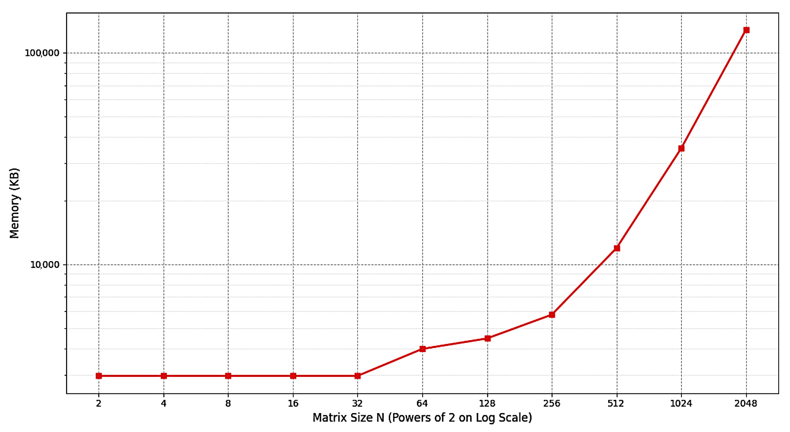
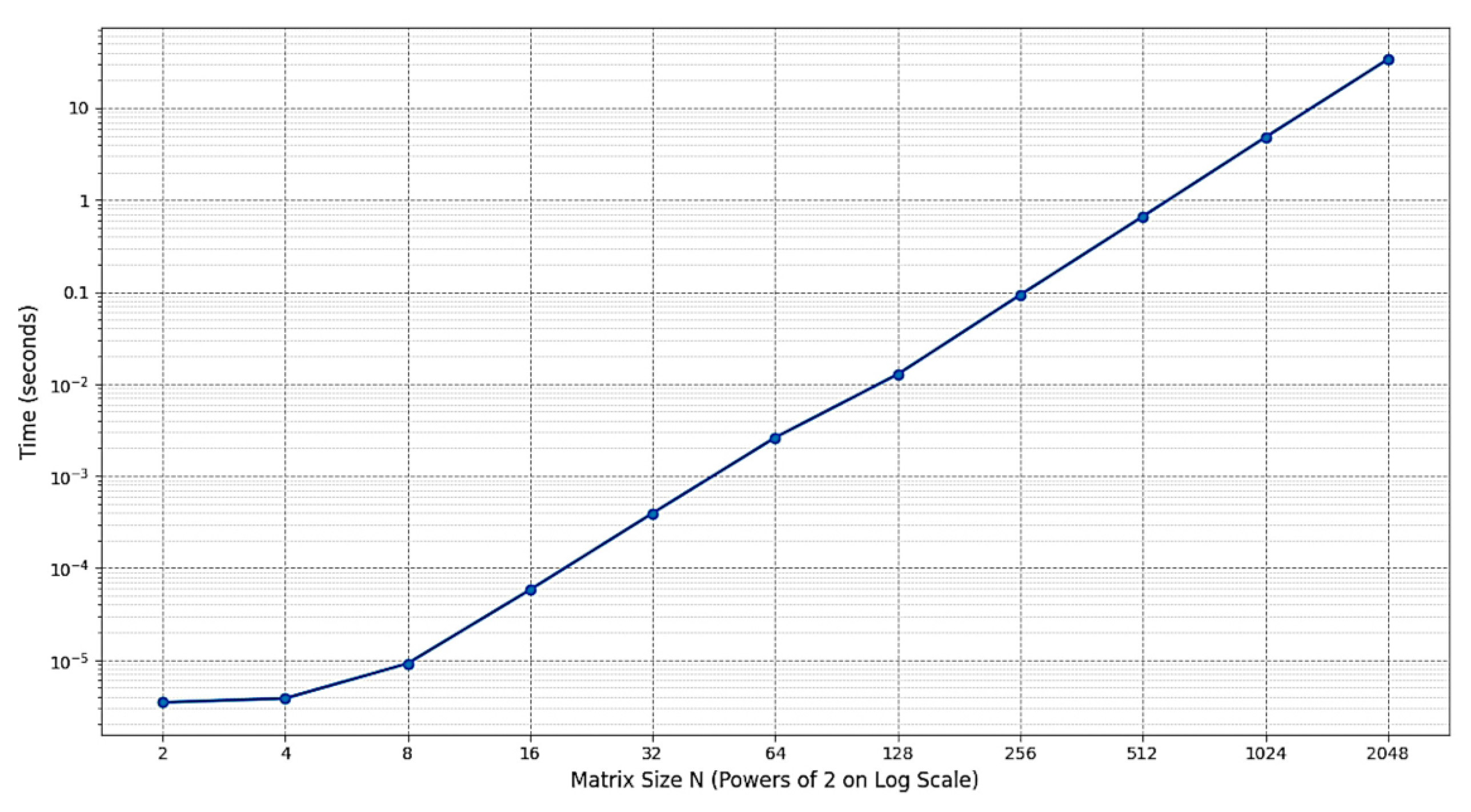
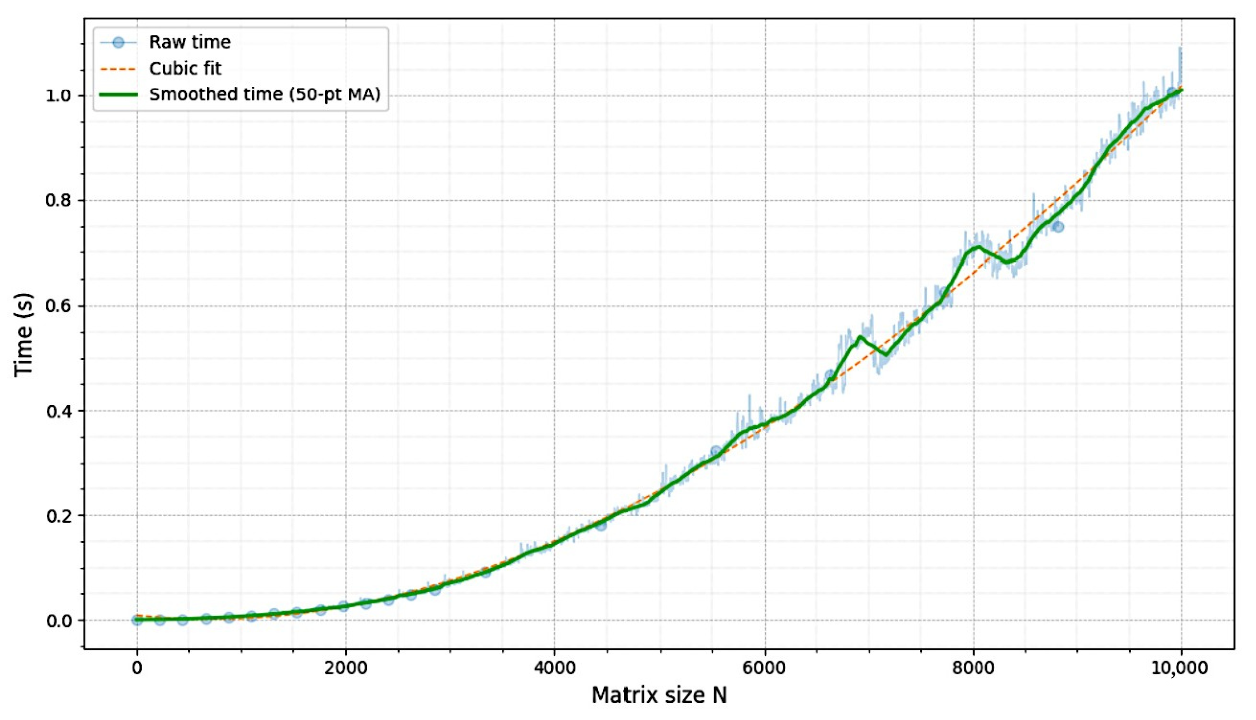
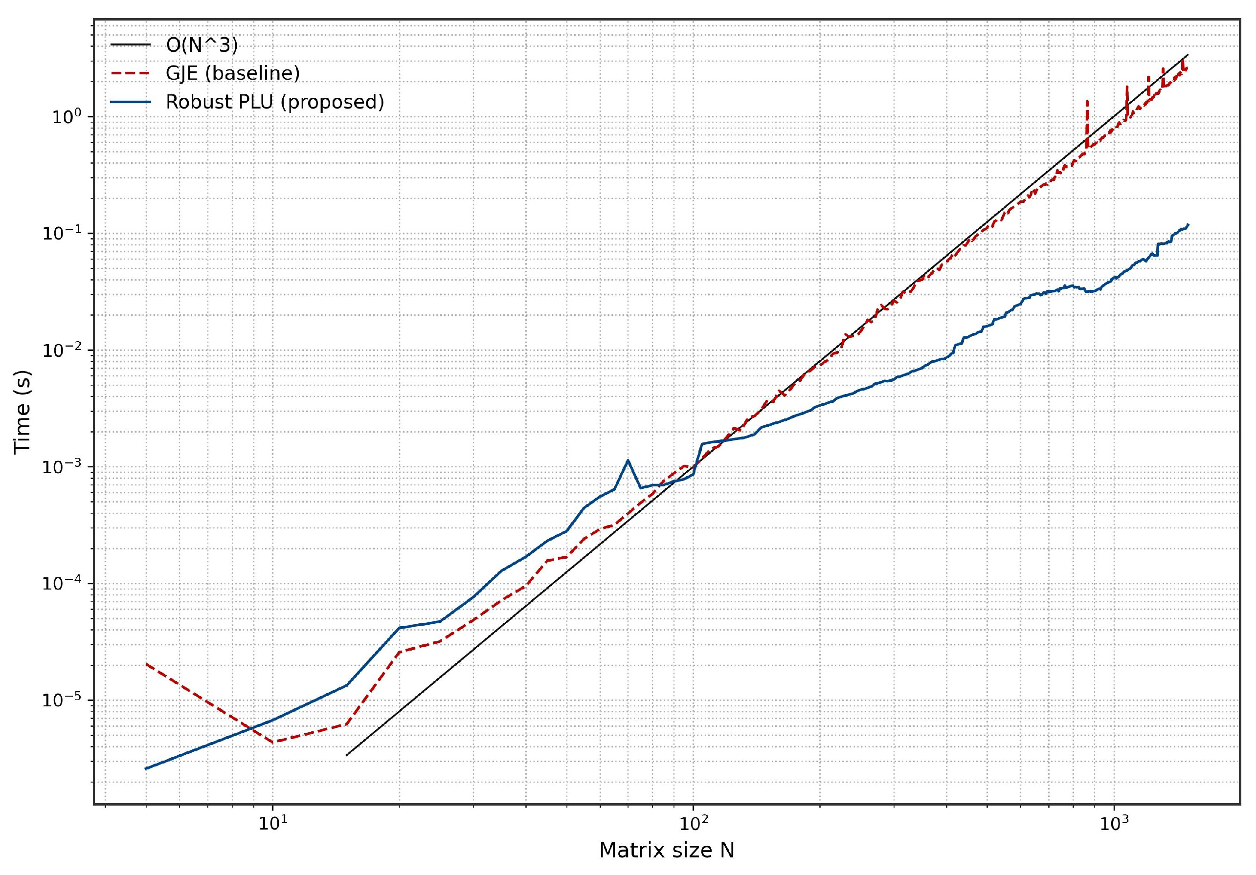
The empirical measurements of the runtime and memory usage for inverting the binary matrices of size $2^n$, $n\le 11$, are shown in Figure 1 and Figure 2, respectively. Both metrics appear to have asymptotically linear growths on the log-log scale plots, suggesting asymptotic complexity, $\mathcal{O}\left(2^{nlog2}\right)$. Furthermore, the empirical runtimes of the proposed blockwise matrix inversion method are compared with the runtimes of the inversion performed using the standard GJE in Figure 3. It can be observed that the proposed method achieves a clear speedup for sufficiently large matrices, and the speedup grows further with the size of the matrix to be inverted. In particular, utilizing Strassen multiplications of sub-blocks reduces the time complexity from $\mathcal{O}\left(n^3\right)$ to $\mathcal{O}\left(n^{2.81}\right)$. It is not as good as the state-of-the art method reported in [2] with $\mathcal{O}\left(n^{2.21}\right)$, but it is still better than the method of Four Russians, which has the time complexity, $\mathcal{O}\left(n^{3/logn}\right)$. Moreover, the peak memory usage is under 7 MB when processing the matrices of a size as large as $N=1400$. Such a memory efficiency can be attributed to the use of the std::vector<bool> data structure for storing the binary matrices.

Algorithm 1: Robust blockwise inversion of a large binary matrix

Input: matrix $\mathit{A}\in F_2^{n\times n}$ Output: inverse matrix ${\mathit{A}}^{-1}$, or ⊥ if $\mathit{A}$ is singular Parameters: base case cutoff $N_0$ 1: function  BinaryInvert($\mathit{A}$,$N_0$) 2:     $n\leftarrow \mathrm{rows}\left(\mathit{A}\right)$ 3:     if $n\le N_0$ then 4:         return GaussJordanInverse(A)    // Base cases 5:     end if 6:     Step 1: Search for pivots 7:     Find index $(r,c):$$A_{r,c}=1$ 8:     if no such index exists then return ⊥    // Matrix is singular 9:     end if 10:   Step 2: Permute to move pivot to $(0,0)$ 11:    ${\mathit{A}}^{\prime }\leftarrow \mathit{P}\mathit{A}\mathbf{Q}$    // $P,Q$ are permutation matrices to swap row $0\leftrightarrow r$, and col $0\leftrightarrow c$ 12:    Partition ${\mathit{A}}^{\prime }$    // rank-1 decomposition $${\mathit{A}}^{\prime }=\left(\begin{array}{cc}1& {\mathit{b}}^T\\ \mathit{c}& \mathit{D}\end{array}\right)$$ 13:    Step 3: Schur complement & recursion 14:     $\mathbf{T}\leftarrow$StrassenMul$(\mathit{c},{\mathit{b}}^T)$ 15:     $S\leftarrow \mathit{D}+\mathit{T}$    // Addition in $F_2$ is XOR 16:     ${\mathit{S}}^{-1}\leftarrow$BinaryInvert$(\mathit{S},N_0)$    // Recursive call 17:     if [ then0.5]${\mathit{S}}^{-1} = \perp$ return ⊥ 18:     end if[0.5] 19:     Step 4: Reconstruct ${\mathit{A}}^{\prime -1}$ 20:        $\mathit{t}\leftarrow$StrassenMul$({\mathit{S}}^{-1},\mathit{c})$ 21:        $\mathit{u}\leftarrow$StrassenMul$({\mathit{b}}^T,{\mathit{S}}^{-1})$ 22:        $\mathit{v}\leftarrow$StrassenMul$({\mathit{b}}^T,\mathit{t})$ 23:        $\alpha \leftarrow 1+{\mathit{v}}_{0,0}$ 24:        Construct $${\mathit{A}}^{\prime -1}=\left(\begin{array}{cc}\alpha & {\mathit{u}}^T\\ \mathit{t}& {\mathit{S}}^{-1}\end{array}\right)$$ 25:     Step 5: Revert permutation 26:        ${\mathit{A}}^{-1}\leftarrow Q{\mathit{A}}^{\prime -1}\mathit{P}$ 27:        return ${\mathit{A}}^{-1}$ 28: end function 29: $\mathbf{Input}\mathbf{:}\mathrm{matrices}\mathit{X},\mathit{Y}$ 30: Output: product $\mathit{C}=\mathit{X}\mathit{Y}$ 31: function StrassenMul($\mathit{X},\mathit{Y}$)    // Strassen matrix multiplication 32:     $n\leftarrow \mathrm{rows}\left(X\right)$ 33:     if $n\le N_0$ or n is odd then 34:         return Mul($\mathbf{X},\mathbf{Y}$)    // standard $\mathcal{O}\left(n^3\right)$ multiplication 35:     end if 36:     Partition $\mathit{X},\mathit{Y}$    // $(n/2\times n/2)$ sub-blocks $$\mathit{X}=\left(\begin{array}{cc}{\mathit{X}}_{11}& {\mathit{X}}_{12}\\ {\mathit{X}}_{21}& {\mathit{X}}_{22}\end{array}\right),\mathit{Y}=\left(\begin{array}{cc}{\mathit{Y}}_{11}& {\mathit{Y}}_{12}\\ {\mathit{Y}}_{21}& {\mathit{Y}}_{22}\end{array}\right)$$ 37:     Compute 7 products 38:        ${\mathit{M}}_1\leftarrow$StrassenMul$({\mathit{X}}_{11}+{\mathit{X}}_{22},{\mathit{Y}}_{11}+{\mathit{Y}}_{22})$ 39:           ...    // similarly for ${\mathit{M}}_2$ through ${\mathit{M}}_7$ 40:        combine ${\mathit{M}}_i$ to form ${\mathit{C}}_{11},{\mathit{C}}_{12},{\mathit{C}}_{21},{\mathit{C}}_{22}$, and then form $\mathit{C}$ 41:     return C 42: end function

Note also that the results shown in Figure 3 suggest that the GJE is as effective as the blockwise recursion for the binary matrices of dimensions up to about $n=100$ due to the overhead of the recursive calls. Hence, the base case sub-matrices can be considered to be relatively large.

Even though the reference implementation in C++ considers specifically the matrices over $\mathrm{GF}\left(2\right)$, the blockwise recursive inversion with the PLU factorization can be readily modified to other fields. Note also that only the computations over finite fields are exact, whereas the algorithms involving the floating point arithmetic operations suffer from the numerical instabilities and numerically ill-conditioned problems. For example, the pivoting used in the GJE must be made more robust for inverting the real-valued matrices. Moreover, the bit-level parallelization can be much more easily exploited for the finite fields than for the real numbers, which has a noticeable impact on the practical runtime and the memory usage of the implemented algorithms.

The matrix multiplications in Strassen’s algorithm can be parallelized to support inverting very large matrices on multi-core computing platforms. For such matrices, the data structures could be further optimized to improve the data locality and to exploit the fast memory-caching mechanisms. Moreover, there can be multiple implementations that are optimized for different matrix sizes, $2^n$. Similar considerations can be assumed for the high-throughput inversions of large matrices that are performed in hardware, for example, using the FPGAs.

3. Enumerating GL(n,2) Groups

The objective now is to exhaustively enumerate the unique elements of the linear group $GL(n,2)$. A naive approach may again exploit the PLU factorization assumed in the previous section. The caveat is how to avoid a considerable redundancy by removing the generated matrix duplications. Ideally, every unique invertible matrix of a given size is generated exactly once. The proposed solution is to consider the Bruhat decomposition theorem to define a unique factorization of every invertible matrix [21]. The key idea is that every invertible matrix can be reduced to exactly one permutation pattern of pivots using the GJE. The theorem can be specifically restated for general linear groups as follows.

Theorem 3  

(Bruhat decomposition of general linear groups). The general linear group, $GL(n,q)$, is a disjoint union of double cosets of the subgroup of upper triangular invertible matrices, $\mathit{B}$, i.e.,

$$GL(n,q)=\underset{\mathit{P}\in {\mathit{S}}_n}{⨆}\mathit{B}\mathit{P}\mathit{B}$$

(11)

where ${\mathit{S}}_n$ is the symmetric group of $(n!)$ permutation matrices and ⊔ denotes the disjoint union.

Theorem 3 allows for partitioning the group $GL(n,2)$ into the disjoint subgroups called Bruhat cells, which are indexed by the permutation matrices. More importantly, every invertible matrix, $\mathit{A}$, has a unique factorization, $\mathit{A}=\mathit{L}\mathit{P}\mathit{U}$, where $\mathit{P}$ is a permutation matrix, and $\mathit{L}$ and $\mathit{U}$ are the lower and the upper triangular matrices, respectively, having non-zero elements that are strictly constrained by the structure of $\mathit{P}$. The uniqueness of this decomposition enables the effective non-redundant enumeration of all invertible matrices of a given size.

In particular, the matrix, $\mathit{L}$, is defined by the so-called inversions of the permutation, $\pi$, of a given permutation matrix, $\mathit{P}$. The inversion is an index pair, $(i,j)$, such that, $i<j$, whereas $\pi \left(i\right)>\pi \left(j\right)$. The matrix $\mathit{L}$ is only allowed to have the non-zero entries at positions $(i,j)$. The number of inversions of permutation $\pi$ is denoted as $\left(\pi \right)=\mathrm{inv}\left(\pi \right)$. Thus, there are $\left(\pi \right)$ elements of matrix $\mathit{L}$ that can be freely selected from a given field, whereas other elements must be zero.

There are $(n!)$ disjoint cells corresponding to one permutation matrix, $\mathit{P}$. The order of each cell is a function of the number of inversions in $\mathit{P}$. For the field of cardinality, q, the cell is a triangular matrix group having the order

$$|C_{\mathit{P}}{|=(q-1)}^n{q}^{\left(\pi \right)}\stackrel{q=2}{=}{2}^{n(n-1)}$$

(12)

where $\left(\pi \right)$ is the cell order. The cell order is a product of the number of unconstrained upper-triangular matrices, $\mathit{U}$, and the number of constrained lower-triangular matrix, $\mathit{L}$.

The enumeration algorithm proceeds by systematically enumerating all permutations, $\pi$, which define the unique permutation matrices, $\mathit{P}$. For $\mathit{P}$, all invertible matrices in the cell, $C_{\mathit{P}}$, are generated. Assuming that the two matrix multiplications to construct a matrix, $\mathit{A}$, have the complexity $\mathcal{O}\left(n^3\right)$ and noting that the double co-sets are disjoint and cover the whole GL group, which has the order given by (2), the overall complexity of the complete enumeration is

$$\mathcal{O}\left(n^3\right)\sum _{\mathit{P}\in {\mathit{S}}_n}|C_{\mathit{P}}|=\mathcal{O}\left(n^3\right)|GL(n,2)|=\mathcal{O}\left(n^3\prod _{k=0}^{n-1}(2^n-2^k)\right)=\mathcal{O}\left(n^3{2}^{n^2}\right).$$

(13)

For comparison, the naive enumeration of the $GL(2,n)$ group using the PLU factorization generates all combinations of the products between $n!$ permutation matrices, and $2^{n(n-1)}$ lower and upper triangular matrices, respectively. The corresponding overall complexity is dominated by the number of these products, each having $\mathcal{O}\left(n^3\right)$ complexity. In addition, each resulting matrix must be checked for whether it has already been generated previously, which has complexity $\mathcal{O}\left(n^2\right)$. Thus, the total complexity of the naive enumeration via the PLU factorization is $\mathcal{O}\left(n!2^{n(n-1)/2}{n}^3\right)=\mathcal{O}\left(n!n^3{2}^{n^2}\right)$. Consequently, even though the complexity of the Bruhat-based enumeration is still exponential, it avoids the factorial scaling of the PLU based enumeration, and at the same time, it is guaranteed to systematically produce a sequence of unique invertible matrices.

Implementation

The proposed algorithm for enumerating all invertible binary matrices is outlined as Algorithm 2 on the next page. The reference C++ implementation again stores the rows of binary matrices in std::vector<int> or in more efficient std::bitset<N> data structures, which encourages the compiled C++ code to use the low-level SIMD instructions. The C++ code is available in [22]. For complexity comparison, the inefficient PLU-based enumeration has also been implemented, and it can be validated only for matrices of size $n\le 5$. In the PLU-based implementation and for small n, the uniqueness of the generated matrices can be automatically enforced by exploiting the std::set data structure with hashing or tree-based indexing. For larger values of n, more advanced data structures are required such as the hash-tries. Even though the complete sets of all lower and upper triangular matrices can be pre-generated, it results in a large memory footprint but faster generation.

The PLU-based enumeration is attractive, since it is already “embarrassingly parallel”, allowing for distributed implementations. There could be other strategies for modifying the PLU-based enumeration so that only unique matrices are implicitly or explicitly generated. It should also be emphasized that the exhaustive enumeration of general linear groups is only feasible for invertible matrices over finite fields, since the group order becomes infinite over infinite fields. Moreover, deciding whether the two real-valued matrices are identical is problematic, as it depends on the floating-point representation of numerical values.

Algorithm 2: Enumeration of $GL(n,2)$ via Bruhat decomposition

Input: integer $n>1$ Output: elements of $GL(n,2)$ 1: function GenGL(n) 2:     $N_U\leftarrow 2^{n(n-1)/2}$    // # unit upper triangular matrices 3:     for all $\pi \in \mathcal{P}$ do    // loop over all $n!$ permutations of $(0,1,\dots ,n-1)$ in set $\mathcal{P}$ 4:         $\mathit{P}\leftarrow$PermutationMatrix$\left(\pi \right)$    // create permutation matrix corresponding to $\pi$ 5:         Step 1: Identify allowed lower inversions 6:         $\mathcal{K}\leftarrow \varnothing$ 7:         for $i\leftarrow 1$ to $n-1$ do 8:            for $j\leftarrow 0$ to $i-1$ do 9:                if $\pi \left[j\right]>\pi \left[i\right]$ then    // standard inversion condition 10:                    $\mathcal{K}\leftarrow \mathcal{K}\cup \left\{\right(i,j\left)\right\}$ 11:                end if 12:            end for 13:         end for 14:         $N_L\leftarrow 2^{\left|\mathcal{K}\right|}$ 15:         Step 2: Iterate over constrained lower matrices 16:         for ${\mathrm{mask}}_L\leftarrow 0$ to $N_L-1$ do 17:            $\mathit{L}\leftarrow {\mathit{I}}_n$    // identity matrix 18:            map bits of ${\mathrm{mask}}_L$ to positions in $\mathcal{K}$ of $\mathit{L}$ 19:            Step 3: Iterate over all upper matrices 20:            ${\mathit{M}}_{\mathrm{partial}}\leftarrow {\mathit{P}}^T\mathit{L}$    // pre-compute 21:            for ${\mathrm{mask}}_U\leftarrow 0$ to $N_U-1$ do 22:                $\mathit{U}\leftarrow$GenerateUnitUpper$(n,{\mathrm{mask}}_U)$ 23:                $\mathit{A}\leftarrow {\mathit{M}}_{\mathrm{partial}}\mathit{U}$ 24:                return A 25:            end for 26:         end for 27:     end for   // loop over permutations 28: end function 29: $\mathbf{Input}\mathbf{:}\mathrm{dimension}\mathit{n}\mathrm{and}\mathrm{parameter}‘\mathrm{mask}’$ 30: Output: unit upper triangular matrix $\mathit{U}$ 31: function GenerateUnitUpper($n,\mathrm{mask}$) 32:     $\mathit{U}\leftarrow {\mathit{I}}_n$, $b\leftarrow 0$ 33:     for $i\leftarrow 0$ to $n-1$ do 34:         for $j\leftarrow i+1$ to $n-1$ do 35:            ${\mathit{U}}_{i,j}\leftarrow (\mathrm{mask}\gg b)\&1$    // right bit-shift 36:            $b\leftarrow b+1$ 37:         end for 38:     end for 39:     return $\mathit{U}$ 40: end function 41: $\mathbf{Input}\mathbf{:}\mathrm{permutation}\pi$ 42: Output: permutation matrix $\mathit{P}$ corresponding to $\pi$ 43: function PermutationMatrix($\pi$) 44:     $\mathit{P}\leftarrow {\mathbf{0}}_{n\times n}$    // all-zeros matrix 45:     for $i\leftarrow 0$ to $n-1$ do 46:         ${\mathit{P}}_{i,\pi \left[i\right]}\leftarrow 1$ 47:     end for 48:     return $\mathit{P}$ 49: end function

4. Repairing Singular Matrices to Become Invertible

In many scenarios, large binary matrices may be nearly invertible; however, they are strictly singular by definition. Such a case can be practically resolved by finding a “closest” invertible matrix that is non-singular. The problem can be formulated as follows.

Problem 1.

Given an $(n\times n)$ binary matrix $\mathit{A}$, find the binary matrix ${\mathit{A}}^{\prime }\in GL(n,2)$ with the minimal Hamming distance, ${\mathcal{D}}_{\mathrm{H}}\left(\mathit{A},{\mathit{A}}^{\prime }\right)$.

Solution 1.

$${\mathit{A}}^{\prime }=\left\{\begin{array}{cc}\mathit{A},& \mathit{A}\in GL(n,2)\\ {arg\; min}_{{\mathit{A}}^{\prime }\in GL(n,2)}{\mathcal{D}}_{\mathrm{H}}\left(\mathit{A},{\mathit{A}}^{\prime }\right),& otherwise.\end{array}\right.$$

(14)

In particular, in the first step, the rank deficiency, $d=n-rank\mathit{A}$, is computed to decide whether $\mathit{A}$ is invertible. If $\mathit{A}$ is already invertible, i.e., $d=0$, the algorithm terminates. Otherwise, the invertible matrix ${\mathit{A}}^{\prime }$, consisting of the Hamming distance precisely, ${\mathcal{D}}_{\mathrm{H}}\left(\mathit{A},{\mathit{A}}^{\prime }\right)=d$, is obtained by flipping exactly d bits in $\mathit{A}$ at defined positions, as explained below.

Note that the matrix repair problem stated above is a variation of the more general maximum rank matrix completion problem studied, for example, in [19]. The rank (i.e., also the rank deficiency) can be computed by the standard GJE. The matrix rank is equal to the number of pivots [9]. Specifically, when transforming the matrix into a row-echelon form, the j-th column does not have a pivot, if there is no row $i\ge j$ such that the element $\mathit{A}(i,j)=1$. The columns without a pivot are referred to as being pivot-free. Equivalently, the row-echelon form contains exactly d all-zero rows. At the same time, it is important to record which rows are swapped during the GJE process. The rows that were swapped and subsequently zeroed are referred as dependent rows, since they are linear combinations of the other rows. The identified pivot-free columns and the dependent rows define the bit positions, which need to be flipped in order to make the original matrix invertible.

Lemma 2  

(Rank change due to single bit-flip). A single bit-flip changes the rank of a binary matrix by at most one.

Proof. 

Let ${\mathit{A}}^{\prime }$ be a square binary matrix obtained by flipping the $(i,j)$ entry of $\mathit{A}$, so that, over $\mathrm{GF}\left(2\right)$, ${\mathit{A}}^{\prime }=\mathit{A}+{\mathit{E}}_{ij}$ and ${\mathit{E}}_{ij}={\mathit{e}}_i{\mathit{e}}_j^T$ have exactly one non-zero element at position $(i,j)$. Considering the combined rows and columns of the matrices $\mathit{A}$ and ${\mathit{E}}_{ij}$, i.e., $\mathrm{span}\{\mathit{A}\cup {\mathit{E}}_{ij}\}=rank(\mathit{A}+{\mathit{E}}_{ij})=rank\mathit{A}+rank{\mathit{E}}_{ij}-rank\{\mathit{A}\cap {\mathit{E}}_{ij}\}=rank\mathit{A}+1-r$, where $r=\{0,1,2\}$, depending on whether the non-zero row and column of ${\mathit{E}}_{ij}$ appears in the span of $\mathit{A}$, we must conclude that $|rank\mathit{A}-rank{\mathit{A}}^{\prime }|\le 1$.    □

Assuming Lemma 2, the task now is to find the set of d bit-flips that reduce the rank deficiency of $\mathit{A}$ to zero so it becomes invertible. These bit-flips are defined by the following theorem.

Theorem 4  

(Minimal bit-flips to make binary matrix invertible). The binary square matrix $\mathit{A}$ with the rank deficiency $d>0$ can be made invertible by performing no less than d bit-flips at the intersection of the dependent rows and the pivot-free columns. These bit-flips can be represented as any of the $(d!)$ permutation matrices of size $(d\times d)$.

Proof. 

The inverse matrix can be obtained by the GJE, which produces the row-echelon form

$$\mathrm{GJE}\left(\mathit{A}\right)=\left(\begin{array}{cc}\mathit{B}& \mathit{C}\\ {\mathbf{0}}_1& {\mathbf{0}}_2\end{array}\right)$$

(15)

where $\mathit{B}$ is a $(r\times r)$ invertible sub-matrix $r=rank\mathit{A}$ and ${\mathbf{0}}_2$ is a $(d\times d)$ all-zero matrix. The last d all-zero rows are dependent swapped rows, and the last d columns are pivot-free columns [9]. The matrix $\mathit{A}$ becomes invertible if ${\mathbf{0}}_2$ in the GJE is replaced by a non-singular matrix; such a matrix must have at least d non-zero elements. For instance, matrix ${\mathbf{0}}_2$ can be replaced with a $(d\times d)$ permutation matrix ${\mathit{P}}_d$. The non-zero elements of ${\mathit{P}}_d$ corresponds to the d bit-flips in $\mathit{A}$, so the GJE of the corresponding perturbed matrix ${\mathit{A}}^{\prime }$ is

$$\mathrm{GJE}\left({\mathit{A}}^{\prime }\right)=\left(\begin{array}{cc}\mathit{B}& \mathit{C}\\ {\mathbf{0}}_1& {\mathit{P}}_d\end{array}\right).$$

(16)

Consequently, $rank{\mathit{A}}^{\prime }=rank\mathit{B}+rank{\mathit{P}}_d=r+d=n$, so ${\mathit{A}}^{\prime }$ is non-singular. Furthermore, by Lemma 2, such a matrix has the minimal possible Hamming distance, ${\mathcal{D}}_{\mathrm{H}}\left({\mathit{A}}^{\prime },\mathit{A}\right)=d$, which is equal to a rank deficiency of $\mathit{A}$.    □

By Lemma 2, every bit-flip can increase the matrix rank by at most one, so the minimum number of bit-flips required to make the matrix invertible is equal to its rank deficiency, d.

Since Theorem 4 allows multiple solutions, the natural question is whether additional constraints could be adopted to narrow down the choices. For instance, it may be desirable to maximize the sparsity by zeroing as many elements as possible, minimize the maximum weight of columns and rows, or make the sub-matrices also invertible.

Note also that Theorem 4.1 in [19] asserts that changing the matrix element at a position corresponding to the basis-avoidable row and column, respectively, increases the matrix rank. Note that in Theorem 4 above, the element positions to increase the matrix rank are referred to as dependent rows and pivot-free columns instead. Such an element change is referred to as rank-one update, and it can be expressed as the product of a column and a row vector. In particular, for binary matrices, there is only one value for how the matrix element can be changed, so the rank-one update can be expressed as

$${\mathit{A}}^{\prime }=\mathit{A}+{\mathit{e}}_i{\mathit{e}}_j^T=\mathit{A}+{\mathit{E}}_{ij}.$$

(17)

For the matrices over other fields, the maximum rank updates are more evolved, since the element values, in addition to their positions, must also be determined [19].

Implementation

The proposed algorithm for repairing singular binary matrices is outlined as Algorithm 3 on the next page. The C++ implementation again uses the std::bitset<N> data structure to store the matrix rows and to allow the compiler to utilize the SIMD instructions for the bit-level parallelism on a single CPU [22]. For example, a binary matrix of size $n=3000$ bits requires approximately $1.13$ MB of memory. The time complexity of making the matrix invertible is dominated by the GJE, which has complexity $\mathcal{O}\left(n^3\right)$. The GJE computations can be at least partially distributed, which is important in high-throughput applications requiring the repair and then inversion of very large binary matrices, such as forward error correction coding, cryptography, and quantized algorithms in machine learning. Moreover, the GJE arithmetic operations for the matrices defined over $\mathrm{GF}\left(2\right)$ are amenable to the fast hardware implementations including, for example, the FPGAs.

Algorithm 3: Singular matrix repair via GJE

Input: matrix $\mathit{A}\in F_2^{n\times n}$ Output: non-singular matrix ${\mathit{A}}^{\prime }=arg\; mind(\mathit{A},{\mathit{A}}^{\prime })$, set of bit-flips F 1: function RepairMatrix($\mathit{A},n$) 2:     $\mathcal{F}\leftarrow \varnothing$ 3:     $(r,{\mathcal{C}}_{\mathrm{pivots}},{\pi }_{\mathrm{rows}})\leftarrow$GaussianElimination$(\mathit{A},n)$ 4:     if $r=n$ then return $\mathit{A}$    // matrix already full-rank 5:     end if 6:     Identify dependent rows: 7:     ${\mathcal{I}}_{\mathrm{dep}}\leftarrow \{{\pi }_{\mathrm{rows}}\left[i\right]\mid r\le i<n\}$    // rows permuted to the bottom are dependent 8:     Identify free columns: 9:     ${\mathcal{J}}_{\mathrm{free}}\leftarrow \{j\in \{0,\dots ,n-1\}\mid j\notin {\mathcal{C}}_{\mathrm{pivots}}\}$ 10:     $d\leftarrow n-r$    // matrix deficiency (nullity) 11:     Perform minimal bit-flips: 12:     for $k\leftarrow 0$ to $d-1$ do 13:         $row\leftarrow {\mathcal{I}}_{\mathrm{dep}}\left[k\right]$ 14:         $col\leftarrow {\mathcal{J}}_{\mathrm{free}}\left[k\right]$ 15:         ${\mathit{A}}_{\mathrm{row},\mathrm{col}}\leftarrow {\mathit{A}}_{\mathrm{row},\mathrm{col}}+1$ 16:         $\mathcal{F}\leftarrow \mathcal{F}\cup \left\{\right(\mathrm{row},\mathrm{col}\left)\right\}$ 17:     end for 18:     return ${\mathit{A}}^{\prime }$ 19: end function 20: $\mathbf{Input}\mathbf{:}\mathrm{matrix}\mathit{M}\mathrm{to\; check\; and\; its\; dimension}\mathit{n}$ 21: Output: matrix rank r, set of pivots ${\mathcal{C}}_{\mathrm{pivots}}$, rows pivoted ${\pi }_{\mathrm{rows}}$ 22: function GaussianElimination($\mathit{M},n$) 23:     ${\mathit{M}}^{\prime }\leftarrow \mathit{M}$    // work on a copy 24:     ${\pi }_{\mathrm{rows}}\leftarrow [0,1,\dots ,n-1]$    // track row permutations 25:     ${\mathcal{C}}_{\mathrm{pivots}}\leftarrow \varnothing$, $r\leftarrow 0$    // current rank 26:     for $j\leftarrow 0$ to $n-1$ do    // iterate over columns 27:         if $r=n$ then break 28:         end if 29:         Step 1: Pivot search 30:         Find smallest $p\ge r$ such that ${\mathit{M}}_{p,j}^{\prime }=1$ 31:         if no such p exists then 32:            continue    // column j is free variable 33:         end if 34:         Step 2: Swap rows    // move pivot to diagonal 35:         SwapRows$({\mathit{M}}^{\prime },r,p)$ 36:         SwapElements$({\pi }_{\mathrm{rows}},r,p)$ 37:         ${\mathcal{C}}_{\mathrm{pivots}}\leftarrow {\mathcal{C}}_{\mathrm{pivots}}\cup \left\{j\right\}$ 38:         Step 3: Elimination 39:         for $i\leftarrow 0$ to $n-1$ do 40:            if $i\ne r$ and ${\mathit{M}}_{i,j}^{\prime }=1$ then 41:                ${\mathit{M}}_i^{\prime }\leftarrow {\mathit{M}}_i^{\prime }+{\mathit{M}}_r^{\prime }$ 42:            end if 43:         end for 44:         $r\leftarrow r+1$ 45:     end for 46:     return $(r,{\mathcal{C}}_{\mathrm{pivots}},{\pi }_{\mathrm{rows}})$ 47: end function

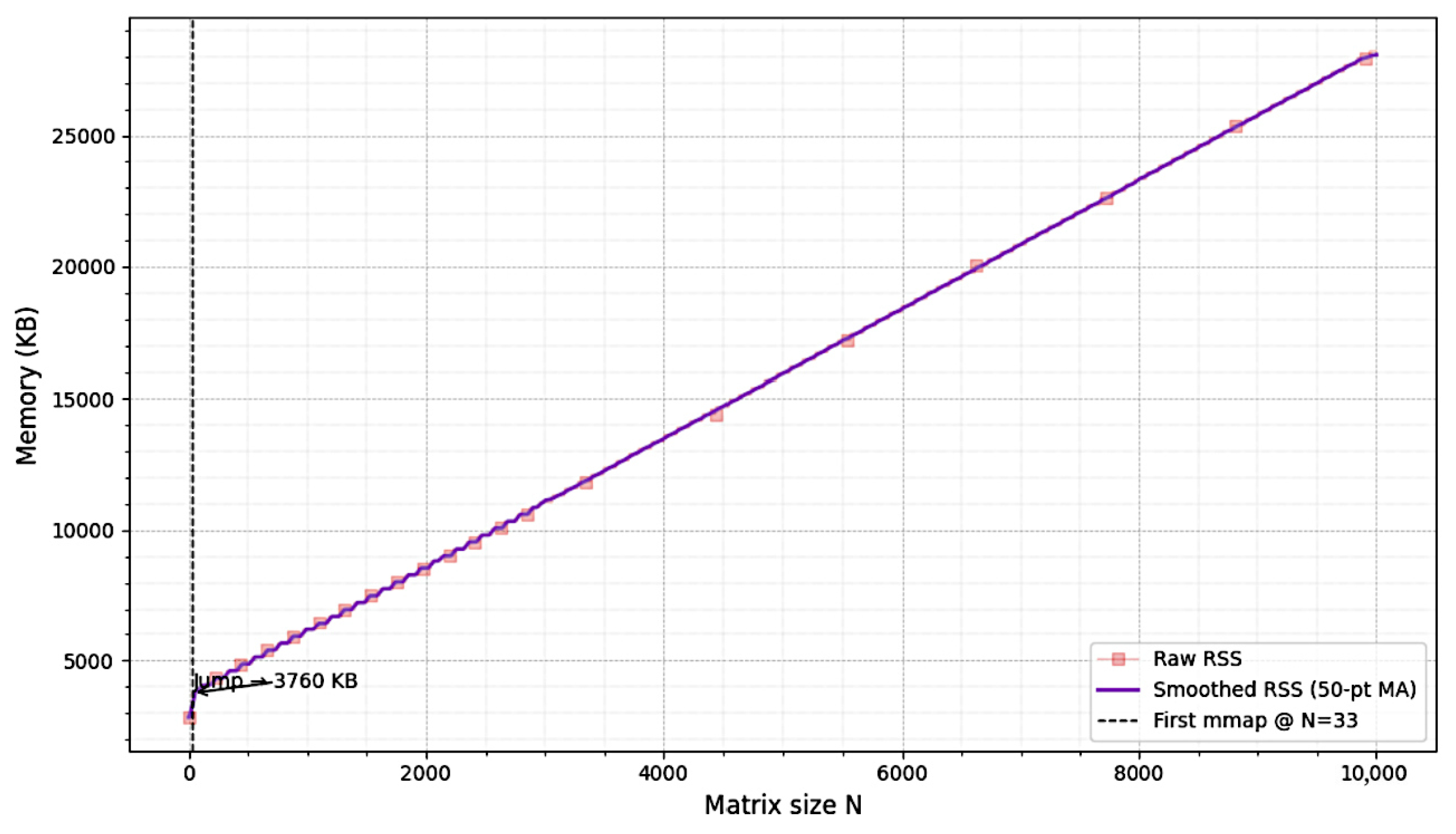
The empirical runtimes and the memory requirements for repairing randomly generated binary matrices to become invertible are shown in Figure 4 and Figure 5, respectively. Note that a binary random matrix is invertible with the probability $|GL(n,2)|/2^{n^2}\doteq 28.9\%$, for $n\gg 1$.

It is unclear whether the required bit-flips to make the binary matrix invertible could be found more directly in order to reduce the cubic cost of the GJE. The complexity of the GJE itself can be reduced by adopting faster matrix multiplications, for example, using the Method of Four Russians and other Strassen-like algorithms [12].

5. Conclusions

This paper investigated three related problems of inverting large binary matrices. Specifically, a robust blockwise matrix inversion was proposed that is based on PLU factorization. The time complexity of this algorithm was evaluated both theoretically and empirically. Surprisingly, the base cases can be assumed to be relatively large when achieving sub-cubic scaling in complexity. Next, it was shown that the enumeration of general linear groups can be carried out much more efficiently by assuming Bruhat decomposition rather than PLU factorization in order to only generate unique invertible matrices. Finally, we showed how to find an invertible binary matrix that is closest to a given singular binary matrix by performing the minimum number of bit-flips at the determined positions. The number of these bit-flips is equal to the rank deficiency of the original matrix. All proposed algorithms were validated to show their correctness. The reference C++ implementation is available in a public Github repository.

The proofs of theorems and lemmas provided in this paper are sketches and not fully rigorous arguments. It is likely that these proofs could be deduced from other known results in linear algebra. It should also be noted that the focus of this paper is on computational and algorithmic problems, and this paper makes no attempts to contribute any fundamental theoretical results in linear algebra. Furthermore, the presented algorithms can be used, in principle, for matrices defined over any finite fields. The implementation for specific fields can be highly optimized, which has a significant impact on the constants used in time and space complexity expressions and which are not shown explicitly in the big-O complexity notation. The single-thread implementation of the algorithms presented in this paper are provided as a reference. This implementation can be further optimized, for example, to support dynamic data structures allocated during the runtime and to allow multi-threaded and multi-processor parallel executions. In general, it would be very desirable to provide low-level highly optimized implementations of the numerical libraries for linear algebra over specific as well as general finite fields, since the number of relevant computing applications is steadily growing.