Chaos in a Generalized Perturbed Lotka–Volterra Model

Abstract

In this paper we investigate the chaos of a generalized perturbed Lotka–Volterra model based on considerations by other studies used in the literature. The model, containing N number of free parameters, could be of interest to specialists working in the fields of biological applications, chemistry, reaction kinetics, biostatistics, games theory, etc. With a specially developed software product, we generate the Melnikov equation $M(t)=0$ and examine all its zeros. This opens up an opportunity for the researcher to correctly understand and formulate the classical Melnikov criterion for the possible occurrence of chaos in the dynamical system. Several simulations are composed. We also demonstrate some specialized modules for investigating the dynamics of the proposed model. We further develop our model using the exponential form of the sine function. Thus, the perturbation can be interpreted as a term dependent on the characteristic function of a probability distribution. Although the original formulation leads to a distribution stated on a discrete domain, we can easily generalize the results for arbitrary distributions. Some particular examples are provided.

1. Introduction

Lotka–Volterra differential systems [1,2] and many of their variants have been used extensively in modelling population dynamics. The publications on this topic are significant and varied (see, for instance, [3,4,5,6,7,8]) and a large number of authors have used computer simulations in their investigations.

In [3], the authors consider systems of interacting species obeying Lotka–Volterra equations and show that periodic attractors may be generated from the equilibrium point in phase space by Hopf bifurcation.

For spiral chaos in a predator–prey model, see [5].

In the studies [4,6,7,8] cited above, the reader can find a considerable volume of research devoted to this classic model.

Scenarios leading to chaos in a forced Lotka–Volterra model are studied in [9].

For the topics of bifurcation and chaos in a periodic predator–prey model, and chaos and Melnikov’s method, see [10,11,12].

A classical predator–prey model is considered in [13] with reference to the case of periodically varying parameters.

Six elementary seasonality mechanisms are identified and analyzed in detail by means of a continuation technique producing complete bifurcation diagrams.

The authors in [14] subject to periodic forcing the classical Volterra predator–prey ecosystem model, which in its unforced state has a globally stable focus as its equilibrium.

The transitions to chaos were found to be either via a Feigenbaum cascade of period-doubling bifurcations or via frequency locking.

For research on order and chaos in ecological systems, see [15].

Following May and Leonard’s [16] considerations on the Gauss–Lotka–Volterra system, the authors in [17] discuss some models of competition between three species.

It is shown that these models exhibit orbits converging to cycles which consist of three saddle points and three orbits connecting them.

For other basic results, see [18,19,20,21,22,23,24,25,26,27].

The dynamics of the modified Lotka–Volterra model with polynomial intervention factors are considered in [28].

In [29], the authors offer a software tool for simulating the dynamics of a new modification of the Lotka–Volterra competition model with “polynomial intervention factors” (monotonically increasing, or monotonically decreasing in the considered interval).

On the uniform stability of impulse Lotka–Volterra type systems with supremums, see [30,31].

The important topics related to the refinement of limit cycle oscillations, response time, and the time–dependent solution to the Lotka–Volterra predator–prey model are the subject of the research presented in [32].

The Lotka–Volterra equations have a long history of use in economic theory and marketing (see for example [33,34]).

Interesting research on the topic of integrating Lotka–Volterra dynamics and gravity modeling for regional population forecasting can be found in [35].

The PhD Thesis in [36] proposes a formal yet flexible framework for the calibration of mathematical models with a particular emphasis on ecosystem modeling.

We are far from claiming that with this brief introduction we have exhausted all current research devoted to this classic model and its basic modifications.

We will conclude this review with the explicit note that regarding the important topic stochastic spatial Lotka–Volterra predator–prey models, the reader can find a relatively complete bibliographic reference in the article in [37].

For the purposes of this study, we will focus on another interesting modification of the Lotka–Volterra model, namely the so-called perturbed Lotka–Volterra model.

Christie, Gopalsamy, and Li [38] consider a slowly varying perturbed three-dimensional Lotka–Volterra system and show that the corresponding unperturbed system has a heteroclinic cycle and a continuous family of periodic orbits.

A special case of the two-dimensional system is

$$\left\{\begin{array}{ccc}{\displaystyle \frac{\mathrm{d}x}{\mathrm{d}t}}\hfill & =& x(c-bx-2dy)+ϵ(l_{1}x+(l_2+l_{3}x)sin(\omega t)),\hfill \\ {\displaystyle \frac{\mathrm{d}y}{\mathrm{d}t}}\hfill & =& y(-c+2bx+dy)+ϵ(l_{1}y+(l_2+l_{3}y)sin(\omega t)),\hfill \end{array}\right.$$

(1)

where $0\le ϵ<1$ is also discussed.

One can derive the following parametric representations for the three heteroclinic orbits.

Let $q_0(t)=(x_0(t),y_0(t))$ be one of the heteroclinic solutions of the first integral of (1) ($ϵ=0$) given by the following (for more details, see precise considerations in [38]):

$$\begin{array}{c}AB:x_0(t)=0;y_0(t)={\displaystyle \frac{c}{d(1+e^{ct})}},\hfill \\ AC:x_0(t)={\displaystyle \frac{c}{b(1+e^{-ct})}};y_0(t)=0,\hfill \\ BC:x_0(t)={\displaystyle \frac{c}{b(1+e^{ct})}};y_0(t)={\displaystyle \frac{c}{d(1+e^{-ct})}}.\hfill \end{array}$$

(2)

(Here, $A(0,0),B(0,{\displaystyle \frac{c}{d}}),C({\displaystyle \frac{c}{b}},0)$ are the saddle points.)

System (1) for $ϵ=0$, $c=0.4;b=0.5;d=0.6$, has the phase portrait shown in Figure 1.

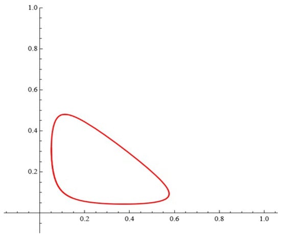
Figure 1. The phase portrait.

Following the results of Wiggins and Holmes [25], the authors in [38] obtain the following explicit representations for the Melnikov integrals [12]:

$$\begin{array}{ccc}{\left.M(t_0)\right|}_{AB}\hfill & =& {\displaystyle {\int }_{-\infty }^{\infty }}{y}_0(t)(c-d{y}_0(t))l_{2}sin(\omega (t+t_0))\mathrm{d}t\hfill \\ & =& {\displaystyle \frac{l_2\pi \omega }{d}}\mathrm{cosech}({\displaystyle \frac{\pi \omega }{c}})sin(\omega t_0);\hfill \end{array}$$

$$\begin{array}{ccc}{\left.M(t_0)\right|}_{AC}\hfill & =& {\displaystyle {\int }_{-\infty }^{\infty }}{x}_0(t)(c-b{x}_0(t))l_{2}sin(\omega (t+t_0))\mathrm{d}t\hfill \\ & =& {\displaystyle \frac{l_2\pi \omega }{b}}\mathrm{cosech}({\displaystyle \frac{\pi \omega }{c}})sin(\omega t_0);\hfill \end{array}$$

$$\begin{array}{ccc}{\left.M(t_0)\right|}_{BC}\hfill & =& l_2{\displaystyle {\int }_{-\infty }^{\infty }}(x_0(t)(c-b{x}_0(t)-2d{y}_0(t))+y_0(t)(c-2b{x}_0(t)-d{y}_0(t)))\mathrm{d}t\hfill \\ \hfill & & -{\displaystyle {\int }_{-\infty }^{\infty }}{x}_0(t)y_0(t)c(l_1+l_{3}sin(\omega (t+t_0)))\mathrm{d}t\hfill \\ \hfill & =& -{\displaystyle \frac{l_1{c}^2}{bd}}-(l_2({\displaystyle \frac{1}{b}}+{\displaystyle \frac{1}{d}})+{\displaystyle \frac{l_{3}c}{bd}})\pi \omega \mathrm{cosech}({\displaystyle \frac{\pi \omega }{c}})sin(\omega t_0).\hfill \end{array}$$

(3)

From (3), Christie, Gopalsamy, and Li [38] show that if $l_2\ne 0$ and

$$|l_1|<\left|{\displaystyle \frac{b+d}{c^2}}{l}_2+{\displaystyle \frac{l_3}{c}}\right|\pi \omega \mathrm{cosech}({\displaystyle \frac{\pi \omega }{c}})$$

then every Melnikov function has simple zeros.

In this paper, we suggest a new class of extended perturbed Lotka–Volterra models of type (1) using multiple periodic terms. Investigations in light of Melnikov’s approach are considered. Several simulations are composed. We demonstrate some modules for investigating the dynamics of the proposed model.

As we mentioned above, we also discuss the model through the characteristic functions of the probability distributions. This is possible since the sine function can be written as a difference between two complex exponents. Although the original model leads to a discrete distribution, we can generalize the results for arbitrary distributions. We consider a three-dimensional Lotka–Volterra model with a zero-powered Gaussian term in the first component, a first-powered Gamma term in the second component, and the second power of the exponential distribution in the third component, among other formulae. Furthermore, we show how a power dependence on the related random variable can be introduced in our scheme.

The plan of this paper is as follows. We state our model in Section 2. Investigations in light of Melnikov’s approach are considered in Section 3. Some simulations are presented in Section 4. One possible application that Melnikov functions (corresponding to the considered differential system) may find in the modeling and synthesis of radiating antenna patterns is also considered. The formulation through the characteristic functions is provided in Section 5. We conclude with Section 6.

2. The New Model

In this paper, we suggest a generalized perturbed Lotka–Volterra model of the type

$$\left\{\begin{array}{ccc}{\displaystyle \frac{\mathrm{d}x}{\mathrm{d}t}}\hfill & =& x(c-bx-2dy)+ϵ(l_{1}x+(l_2+l_{3}x){\displaystyle \sum _{i=1}^N}{a}_{i}sin(i\omega t)),\hfill \\ {\displaystyle \frac{\mathrm{d}y}{\mathrm{d}t}}\hfill & =& y(-c+2bx+dy)+ϵ(l_{1}y+(l_2+l_{3}y){\displaystyle \sum _{i=1}^N}{a}_{i}sin(i\omega t)),\hfill \end{array}\right.$$

(4)

where $0\le ϵ<1$, $a_i\ge 0;i=1,2,\dots ,N$ and N is an integer.

Evidently, the model, containing N number of free parameters, could be of interest to specialists working in the fields of biological applications, reaction kinetics, biostatistics, games theory, etc.

3. Considerations in Light of Melnikov’s Approach

System (4) is of the form

$$\begin{array}{ccc}{\displaystyle \frac{\mathrm{d}x}{\mathrm{d}t}}\hfill & =& f_1(x,y)+ϵg_1(x,y,t),\hfill \\ {\displaystyle \frac{\mathrm{d}y}{\mathrm{d}t}}\hfill & =& f_2(x,y)+ϵg_2(x,y,t).\hfill \end{array}$$

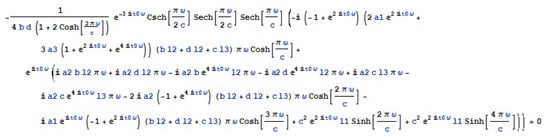
The Melnikov function [12] corresponding to system (4) is of the form

$$\begin{array}{c}M(t_0)={\displaystyle {\int }_{-\infty }^{\infty }}f(q_0(t))\wedge g(q_0(t),t+t_0)e^{-{\int }_0^{t}traceDf(q_0(s))\mathrm{d}s}\mathrm{d}t\hfill \\ ={\displaystyle {\int }_{-\infty }^{\infty }}\left(x_0(t)(c-b{x}_0(t)-2d{y}_0(t))(l_1{y}_0(t)+(l_2+l_3{y}_0(t)){\displaystyle \sum _{i=1}^N}{a}_{i}sin(i\omega (t+t_0)))\right.\hfill \\ +\left.y_0(t)(c-2b{x}_0(t)-d{y}_0(t))(l_1{x}_0(t)+(l_2+l_3{x}_0(t)){\displaystyle \sum _{i=1}^N}{a}_{i}sin(i\omega (t+t_0)))\right)B(t)\mathrm{d}t.\hfill \end{array}$$

(5)

It is easy to see that

$$B(t)=e^{-{\displaystyle {\int }_0^t\left(c-2b{x}_0(s)-2d{y}_0(s)-c+2b{x}_0(s)+2d{y}_0(s)\right)\mathrm{d}s}}=1.$$

The Melnikov function can be represented in another way, using the following familiar equality:

$$sin(i\omega (t+t_0))=sin(i\omega t)cos(i\omega t_0)+cos(i\omega t)sin(i\omega t_0).$$

We will not dwell on this question here.

For us, it is more important to note that such a representation is more appropriate and can be used directly by users of a corresponding specialized module implemented, for example, in CAS Mathematica 11.

It is known (the so-called Melnikov criterion) that if $M(t_0)=0$ and ${\displaystyle \frac{M(t_0)}{\mathrm{d}{t}_0}}\ne 0$ for some $t_0$ and some sets of parameters, then chaos occurs in the considered differential model.

3.1. The Case $N=2$

Proposition 1.

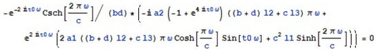
If $N=2$, then the roots of Melnikov function $M(t_0)$ are given as solutions of the equation $M(t_0)=0$ (see Figure 2):

Figure 2. The equation $M(t_0)=0$ (from Proposition 1).

Example 1.

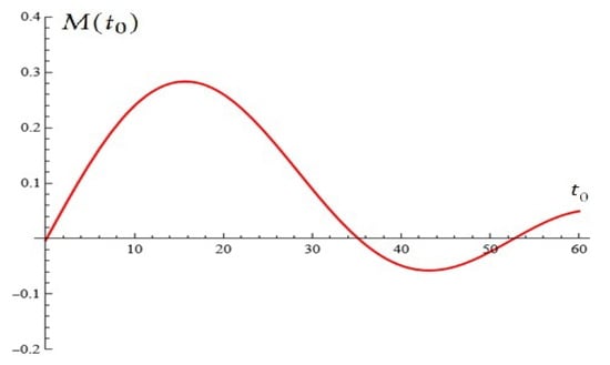
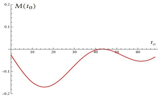
For $N=2$, $b=0.2,c=0.1,d=1.6$, $\omega =0.06,l_1=0.1$, $l_2=-0.5,l_3=4.2,a_1=1.9,a_2=6.1$, the Melnikov function $M(t_0)=0$ is depicted in Figure 3.

Figure 3. For $N=2$, $b=0.2,c=0.1,d=1.6$, $\omega =0.06,l_1=0.1,l_2=-0.5,l_3=4.2,a_1=1.9$, $a_2=6.1$ the Melnikov function $M(t_0)=0$ has simple roots (from Proposition 1).

Example 2.

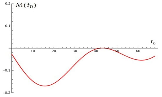
For $N=2$, $b=0.2,c=0.1,d=1.6$, $\omega =0.06,l_1=0.86$, $l_2=-0.1,l_3=4.2,a_1=1.9,a_2=6.1$, the Melnikov function $M(t_0)=0$ is depicted in Figure 4.

Figure 4. For $N=2$, $b=0.2,c=0.1,d=1.6$, $\omega =0.06,l_1=0.86,l_2=-0.1,l_3=4.2,a_1=1.9$, $a_2=6.1$, the Melnikov function $M(t_0)=0$ has root $t_0\approx 42.24$ (with multiplicity two) (from Proposition 1).

3.2. The Case $N=3$

Proposition 2.

If $N=3$, then the roots of the Melnikov function $M(t_0)$ are given as solutions of the equation $M(t_0)=0$ (see Figure 5).

Figure 5. The equation $M(t_0)=0$ (from Proposition 2).

Example 3.

For $N=3$, $b=0.17,c=0.12,d=1.04$, $\omega =0.046,l_1=0.12$, $l_2=-0.11,l_3=1.767,a_1=0.2,a_2=3.1,a_3=1$, the Melnikov function $M(t_0)=0$ is depicted in Figure 6.

Figure 6. For $N=3$, $b=0.17,c=0.12,d=1.04$, $\omega =0.046,l_1=0.12,l_2=-0.11,l_3=1.767$, $a_1=0.2,a_2=3.1,a_3=1$, the Melnikov function $M(t_0)=0$ has root $t_0\approx 50$ (with multiplicity two); (from Proposition 2).

From the above examples, the reader can formulate the corresponding Melnikov criterion for the occurrence of chaos in the considered dynamic system for some N.

4. Some Simulations

We will look at some interesting simulations on model (4):

Example 4.

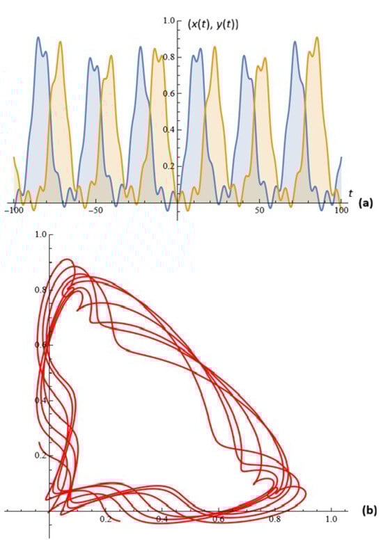
For given $N=1$, $\omega =1$, $c=b=d=0.5$, $l_1=-0.001$, $l_2=1$, $l_3=0$, $ϵ=0.05$, and $a_1=1$, the simulations on system (4) for $x_0=0$; $y_0=0$ are depicted in Figure 7.

Figure 7. (a) The solutions of system (4); (b) phase space (Example 4).

Example 5.

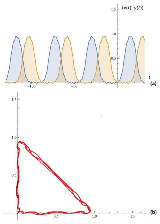
For given $N=3$, $\omega =1$, $c=b=d=0.5$, $l_1=-0.001$, $l_2=1$, $l_3=0$, $ϵ=0.05$, $a_1=0.1$, $a_2=0.5$, and $a_3=0.1$, the simulations on system (4) for $x_0=0$; $y_0=0$ are depicted in Figure 8.

Figure 8. (a) The solutions of system (4); (b) phase space (Example 5).

Example 6.

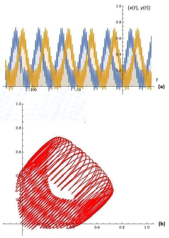
For given $N=5$, $\omega =1$, $c=b=d=0.5$, $l_1=-0.001$, $l_2=1$, $l_3=0$, $ϵ=0.05$, $a_1=0.1$, $a_2=0.5$, $a_3=0.1$, $a_4=9.2$, and $a_5=0.1$, the simulations on system (4) for $x_0=0$; $y_0=0$ are depicted in Figure 9.

Figure 9. (a) The solutions of system (4); (b) phase space (Example 6).

Example 7.

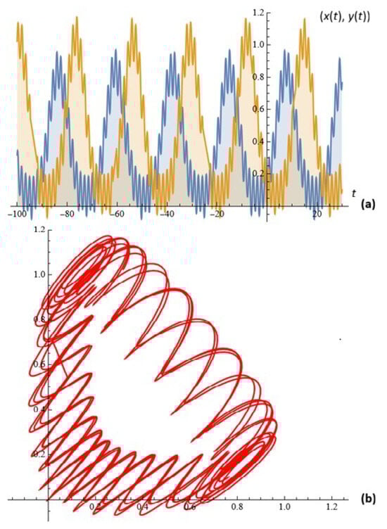
For given $N=7$, $\omega =1$, $c=0.6$, $b=0.5$, $d=0.4$, $l_1=-0.001$, $l_2=1$, $l_3=0.03$, $ϵ=0.05$, $a_1=0.11$, $a_2=0.51$, $a_3=0.11$, $a_4=9.23$, $a_5=0.14$, $a_6=0.7$, and $a_7=0.2$, the simulations on system (4) for $x_0=0$; $y_0=0$ are depicted in Figure 10.

Figure 10. (a) The solutions of system (4); (b) phase space (Example 7).

Example 8.

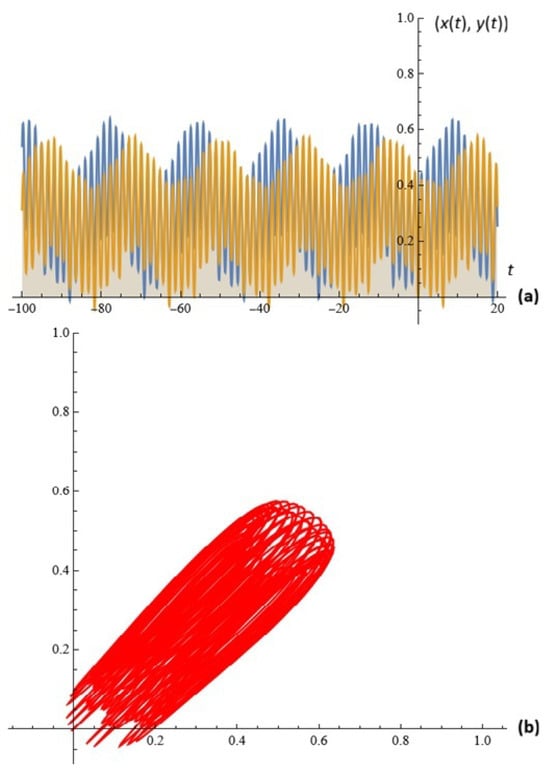
For given $N=9$, $\omega =1$, $c=0.55$, $b=0.45$, $d=0.55$, $l_1=-0.002$, $l_2=1.01$, $l_3=0$, $ϵ=0.085$, $a_1=0.1$, $a_2=0.5$, $a_3=0.1$, $a_4=9.2$, $a_5=0.1$, $a_6=a_7=a_8=0$, and $a_9=0.9$, the simulations on system (4) for $x_0=0$; $y_0=0$ are depicted in Figure 11.

Figure 11. (a) The solutions of system (4); (b) phase space (Example 8).

With Examples 4–8, we demonstrate simulations of generated chaos in the new model.

Remark 1.

In our previous publications, we discussed a possible application of the Melnikov functions (corresponding to various differential systems) in modeling and synthesis of radiation antenna diagrams. We will not dwell on these issues here.

The reader can find sufficient information in the articles [39,40,41].

We will consider only some numerical examples of the possible use of the Melnikov polynomial corresponding to the generalized differential model considered in this article.

We define the hypothetical normalized antenna factor as follows: $M^{*}(\theta )={\displaystyle \frac{1}{D}}|M(Kcos\theta +k_1)|$, where θ is the azimuth angle; $K=kd;k={\displaystyle \frac{2\pi }{\lambda }};\lambda$ is the wave length; d is the distance between emitters; and $k_1$ is the phase difference.

Example 9.

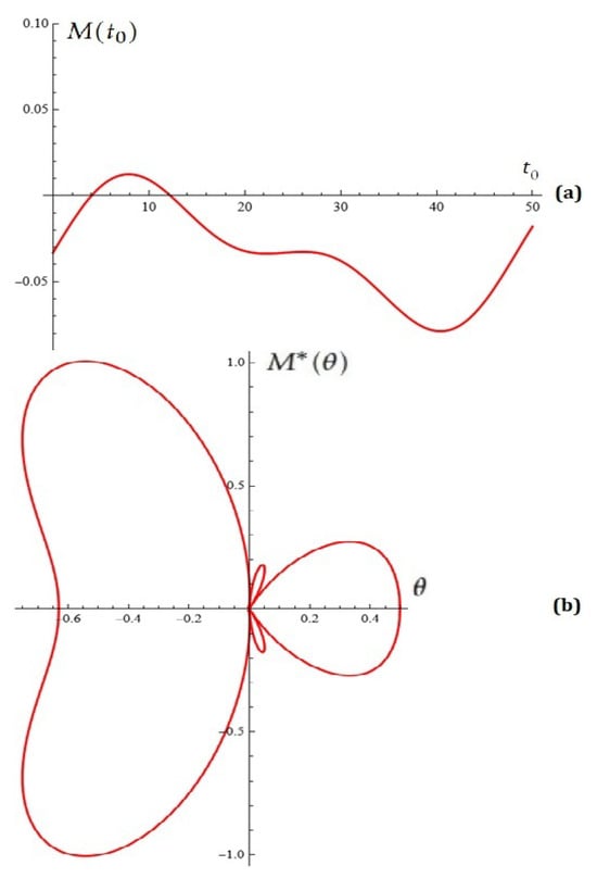
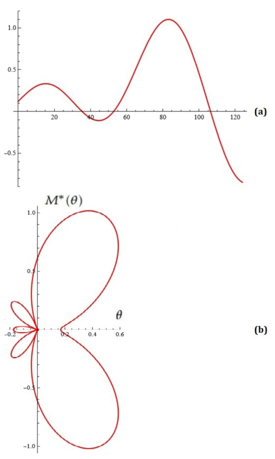
For fixed $N=2$, $k=20$, $k_1=3$, $\omega =0.13$, $a_1=1.09$, $a_2=8.1$, $b=0.25$, $c=0.124$, $d=1.11$, $l_1=0.6$, $l_2=-0.1$, and $l_3=-1.2$, the Melnikov function and Melnikov antenna factor are depicted in Figure 12.

Figure 12. (a) The Melnikov function; (b) Melnikov antenna factor (Example 9).

Example 10.

For fixed $N=3$, $k=30$, $k_1=3$, $\omega =0.03$, $a_1=1.1$, $a_2=-2.1$, $a_3=3.2$, $b=0.17$, $c=0.12$, $d=0.14$, $l_1=-0.2$, $l_2=-0.15$, and $l_3=-0.1$, the Melnikov function and Melnikov antenna factor are depicted in Figure 13.

Figure 13. (a) The Melnikov function; (b) Melnikov antenna factor (Example 10).

Of course, this relatively new idea of justification and right to exist is subject to serious research by specialists working in this scientific direction.

Remark 2.

The following slowly time-varying periodically perturbed Lotka–Volterra system is considered in [38]:

$$\left\{\begin{array}{ccc}{\displaystyle \frac{\mathrm{d}x}{\mathrm{d}t}}\hfill & =& x(c-bx-2dy+az)+ϵ(l_{1}x+(l_2+l_{3}x)sin(\omega t)),\hfill \\ {\displaystyle \frac{\mathrm{d}y}{\mathrm{d}t}}\hfill & =& y(-c+2bx+dy-az)+ϵ(l_{1}y+(l_2+l_{3}y)sin(\omega t)),\hfill \\ {\displaystyle \frac{\mathrm{d}z}{\mathrm{d}t}}\hfill & =& ϵz(l_4+l_{5}sin(\omega t)-l_{6}x+l_{7}y-l_{8}z),\hfill \end{array}\right.$$

(6)

where $0<ϵ\le 1$ denotes the perturbation parameter, $\omega >0$ is the frequency of the perturbation, $a,b,c,d>0$, and $l_j;j=1,\dots ,8$ are real parameters.

We suggest a generalized perturbed Lotka–Volterra system of the type

$$\left\{\begin{array}{ccc}{\displaystyle \frac{\mathrm{d}x}{\mathrm{d}t}}\hfill & =& x(c-bx-2dy+az)+ϵ(l_{1}x+(l_2+l_{3}x){\displaystyle \sum _{i=1}^N}{a}_{i}sin(i\omega t)),\hfill \\ {\displaystyle \frac{\mathrm{d}y}{\mathrm{d}t}}\hfill & =& y(-c+2bx+dy-az)+ϵ(l_{1}y+(l_2+l_{3}y){\displaystyle \sum _{i=1}^N}{a}_{i}sin(i\omega t)),\hfill \\ {\displaystyle \frac{\mathrm{d}z}{\mathrm{d}t}}\hfill & =& ϵz(l_4+l_5{\displaystyle \sum _{i=1}^N}{a}_{i}sin(i\omega t)-l_{6}x+l_{7}y-l_{8}z),\hfill \end{array}\right.$$

(7)

where $0\le ϵ<1$, $a_i\ge 0;i=1,2,\dots ,N$ and N is an integer.

The study of the system in light of Melnikov’s theory can be carried out following the considerations in [38] and the present article, and for this reason we will omit it here.

We will dwell on some interesting examples.

Example 11.

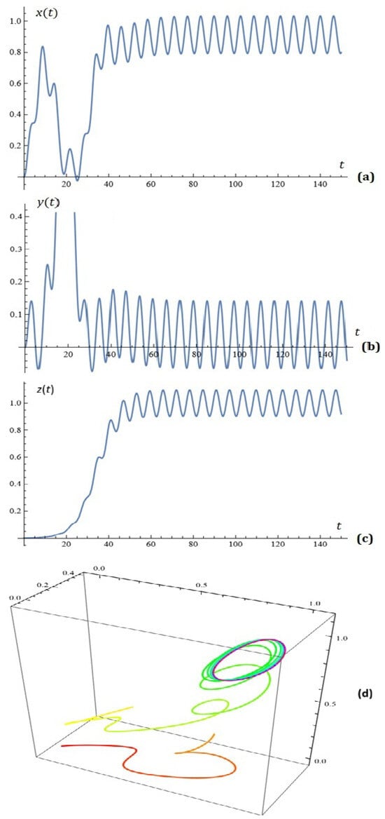
For given $N=2$, $\omega =1$, $c=0.5$, $b=0.5$, $d=0.5$, $l_1=-0.00001$, $l_2=1$, $l_3=0$, $l_4=1$, $l_5=1$, $l_6=0$, $l_7=0$, $l_8=1$, $ϵ=0.2$, $a=0.5$, $a_1=0.495$, and $a_2=0.01$, the simulations on system (7) for $x_0=0$; $y_0=0$; $z_0=0.001$ are depicted in Figure 14.

Figure 14. (a) $x(t)$ component of the solution of system (7); (b) $y(t)$ component of the solution of system (7); (c) $z(t)$ component of the solution of system (7); (d) phase space (Example 11).

Example 12.

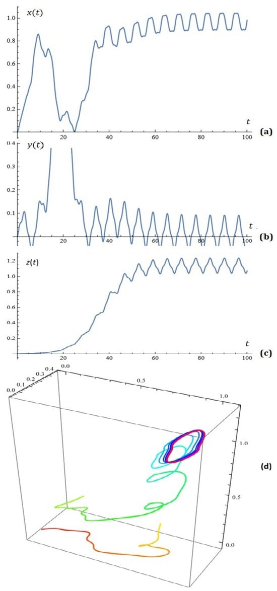
For given $N=4$, $\omega =1.01$, $c=0.5$, $b=0.5$, $d=0.5$, $l_1=-0.00001$, $l_2=0.91$, $l_3=0.11$, $l_4=1.12$, $l_5=1.01$, $l_6=0.1$, $l_7=0.2$, $l_8=0.9$, $ϵ=0.15$, $a=0.5$, $a_1=0.495$, $a_2=0.01$, $a_3=0.295$, and $a_4=0.05$, the simulations on system (7) for $x_0=0$; $y_0=0$; $z_0=0.002$ are depicted in Figure 15.

Figure 15. (a) $x(t)$ component of the solution of system (7); (b) $y(t)$ component of the solution of system (7); (c) $z(t)$ component of the solution of system (7); (d) phase space (Example 12).

5. A Construction Based on Characteristic Functions

We shall discuss now a possible generalization of model (4) based on the characteristic functions of the probability distributions. Let $A={\sum }_{j=1}^N{a}_j$ and ${\overline{a}}_j={\displaystyle \frac{a_J}{A}}$. Thus, we can view the constant ${\overline{a}}_j$ as the probability of a random variable $\xi$ defined on the set $\left\{1,2,\dots ,N\right\}$ to be equal to j. Let its characteristic function be $\psi \left(x\right)$. Using the exponential presentation of the sine function,

$$sin\left(\alpha \right)={\displaystyle \frac{e^{i\alpha }-e^{-i\alpha }}{2i}},$$

(8)

we transform the periodic part of dynamics (4) into

$$\begin{array}{cc}\hfill \sum _{j=1}^N{a}_{j}sin\left(j\omega t\right)& =A\sum _{j=1}^N{\overline{a}}_j{\displaystyle \frac{e^{ij\omega t}-e^{-ij\omega t}}{2i}}\hfill \\ \hfill & ={\displaystyle \frac{A}{2i}}\left(\mathbb{E}\left[e^{i\xi \omega t}\right]-\mathbb{E}\left[e^{-i\xi \omega t}\right]\right)\hfill \\ \hfill & =A{\displaystyle \frac{\psi \left(\omega t\right)-\psi \left(-\omega t\right)}{2i}}.\hfill \end{array}$$

(9)

We can make two main conclusions. First, the domain of the random variable is not important, i.e., we can generalize the sum of N-terms as an integral. And second, keeping in mind that the characteristic function is always well-defined, we can use an arbitrary random variable. Something more, we can use different random variables for x- and y-dynamics. Let these random variables be defined on the domain $\Omega$ (or on its parts)—we shall denote them by ${\xi }_1$ and ${\xi }_2$. Also, let the related characteristic functions be ${\psi }_1\left(·\right)$ and ${\psi }_2\left(·\right)$. Thus, the Lotka–Voltera-type model (4) can be rewritten as

$$\begin{array}{cc}\hfill {\displaystyle \frac{\mathrm{d}x}{\mathrm{d}t}}& =x\left(c-bx-2dy\right)+ϵ\left(l_{1}x+A_1\left(l_2+l_{3}x\right)\underset{\gamma \in \Omega }{\int }sin\left({\xi }_1\left(\gamma \right)\omega t\right)\mathbb{P}\left(d\gamma \right)\right),\hfill \\ \hfill {\displaystyle \frac{\mathrm{d}y}{\mathrm{d}t}}& =y\left(-c+2bx+dy\right)+ϵ\left(l_{1}y+A_2\left(l_2+l_{3}y\right)\underset{\gamma \in \Omega }{\int }sin\left({\xi }_2\left(\gamma \right)\omega t\right)\mathbb{P}\left(d\gamma \right)\right)\hfill \end{array}$$

(10)

or equivalently as

$$\begin{array}{cc}\hfill {\displaystyle \frac{\mathrm{d}x}{\mathrm{d}t}}& =x\left(c-bx-2dy\right)+ϵ\left(l_{1}x+A_1\left(l_2+l_{3}x\right){\displaystyle \frac{{\psi }_1\left(\omega t\right)-{\psi }_1\left(-\omega t\right)}{2i}}\right),\hfill \\ \hfill {\displaystyle \frac{\mathrm{d}y}{\mathrm{d}t}}& =y\left(-c+2bx+dy\right)+ϵ\left(l_{1}y+A_2\left(l_2+l_{3}y\right){\displaystyle \frac{{\psi }_2\left(\omega t\right)-{\psi }_2\left(-\omega t\right)}{2i}}\right).\hfill \end{array}$$

(11)

The Melnikov integral (5) can be rewritten as

$$M\left(t_0\right)={\int }_{-\infty }^{\infty }\left(\begin{array}{c}{A}_1{x}_0\left(t\right)\left(c-b{x}_0\left(t\right)-2d{y}_0\left(t\right)\right)\hfill \\ \times \left(l_1{y}_0\left(t\right)+\left(l_2+l_3{y}_0\left(t\right)\right){\displaystyle \frac{{\psi }_1\left(\omega \left(t+t_0\right)\right)-{\psi }_1\left(-\omega \left(t+t_0\right)\right)}{2i}}\right)\hfill \\ +A_2{y}_0\left(t\right)\left(c-2b{x}_0\left(t\right)-d{y}_0\left(t\right)\right)\hfill \\ \times \left(l_1{x}_0\left(t\right)+\left(l_2+l_3{x}_0\left(t\right)\right){\displaystyle \frac{{\psi }_2\left(\omega \left(t+t_0\right)\right)-{\psi }_2\left(-\omega \left(t+t_0\right)\right)}{2i}}\right)\hfill \end{array}\right)\mathrm{d}t.$$

(12)

We shall give now two examples based on three important distributions—Gaussian, Gamma, and exponential ones. The first one is defined on the whole real line, whereas the second and third ones are defined on its positive part. The probability density functions that appear as $\mathbb{P}\left(d\gamma \right)$ in dynamics (10) are

$$\begin{array}{cc}\hfill f_1\left(z\right)& ={\displaystyle \frac{1}{\sqrt{2\pi {\sigma }^2}}}{e}^{-{\displaystyle \frac{{\left(z-\mu \right)}^2}{2{\sigma }^2}}},\hfill \\ \hfill f_2\left(z\right)& ={\displaystyle \frac{1}{\Gamma \left(\alpha \right){\theta }^{\alpha }}}{z}^{\alpha -1}{e}^{-{\displaystyle \frac{z}{\theta }}},\hfill \\ \hfill f_3\left(z\right)& =\lambda e^{-\lambda z}.\hfill \end{array}$$

(13)

The related characteristic functions are

$$\begin{array}{cc}\hfill {\Psi }_1\left(x\right)& =e^{i\mu x-{\displaystyle \frac{{\sigma }^2{x}^2}{2}}},\hfill \\ \hfill {\Psi }_2\left(x\right)& ={\left(1-i\theta x\right)}^{-\alpha },\hfill \\ \hfill {\Psi }_2\left(x\right)& ={\displaystyle \frac{\lambda }{\lambda -ix}}.\hfill \end{array}$$

(14)

To use generalization (11), we need to obtain the term $\psi \left(x\right)-\psi \left(-x\right)$ for the above-mentioned three distributions. We have

$$\begin{array}{cc}\hfill {\Psi }_1\left(x\right)-{\Psi }_1\left(-x\right)& =e^{i\mu x-{\displaystyle \frac{{\sigma }^2{x}^2}{2}}}-e^{-i\mu x-{\displaystyle \frac{{\sigma }^2{x}^2}{2}}}\hfill \\ \hfill & =e^{-{\displaystyle \frac{{\sigma }^2{x}^2}{2}}}\left(e^{i\mu x}-e^{-i\mu x}\right)\hfill \\ \hfill & =2i{e}^{-{\displaystyle \frac{{\sigma }^2{x}^2}{2}}}sin\left(\mu x\right).\hfill \end{array}$$

(15)

for the Gaussian distribution,

$$\begin{array}{cc}\hfill & {\Psi }_2\left(x\right)-{\Psi }_2\left(-x\right)={\left(1-i\theta x\right)}^{-\alpha }-{\left(1+i\theta x\right)}^{-\alpha }\hfill \\ \hfill & =\sqrt{{\left(1+{\theta }^2{x}^2\right)}^{-\alpha }}{\left({\displaystyle \frac{1}{\sqrt{1+{\theta }^2{x}^2}}}-i{\displaystyle \frac{\theta x}{\sqrt{1+{\theta }^2{x}^2}}}\right)}^{-\alpha }\hfill \\ \hfill & -\sqrt{{\left(1+{\theta }^2{x}^2\right)}^{-\alpha }}{\left({\displaystyle \frac{1}{\sqrt{1+{\theta }^2{x}^2}}}+i{\displaystyle \frac{\theta x}{\sqrt{1+{\theta }^2{x}^2}}}\right)}^{-\alpha }\hfill \\ \hfill & =\sqrt{{\left(1+{\theta }^2{x}^2\right)}^{-\alpha }}{\left(cos\left(-arccos\left({\displaystyle \frac{1}{\sqrt{1+{\theta }^2{x}^2}}}\right)\right)+isin\left(-arccos\left({\displaystyle \frac{1}{\sqrt{1+{\theta }^2{x}^2}}}\right)\right)\right)}^{-\alpha }\hfill \\ \hfill & -\sqrt{{\left(1+{\theta }^2{x}^2\right)}^{-\alpha }}{\left(cos\left(arccos\left({\displaystyle \frac{1}{\sqrt{1+{\theta }^2{x}^2}}}\right)\right)+isin\left(arccos\left({\displaystyle \frac{1}{\sqrt{1+{\theta }^2{x}^2}}}\right)\right)\right)}^{-\alpha }\hfill \\ \hfill & =-2i\sqrt{{\left(1+{\theta }^2{x}^2\right)}^{-\alpha }}sin\left(\alpha arccos\left({\displaystyle \frac{1}{\sqrt{1+{\theta }^2{x}^2}}}\right)\right).\hfill \end{array}$$

(16)

for the Gamma one, and

$$\begin{array}{cc}\hfill {\Psi }_3\left(x\right)-{\Psi }_3\left(-x\right)& ={\displaystyle \frac{\lambda }{\lambda -ix}}-{\displaystyle \frac{\lambda }{\lambda +ix}}\hfill \\ \hfill & ={\displaystyle \frac{2i\lambda x}{{\lambda }^2+x^2}}.\hfill \end{array}$$

(17)

for the exponential distribution.

We shall give two examples to illustrate the suggested model. In the first one, the periodic part of the x-perturbation shall be driven by the Gaussian term (15), whereas the Gamma one (16) shall be used for the y-dynamics. Thus, model (11) turns into

$$\begin{array}{cc}\hfill {\displaystyle \frac{\mathrm{d}x}{\mathrm{d}t}}& =x\left(c-bx-2dy\right)+ϵ\left(l_{1}x+A_1\left(l_2+l_{3}x\right)e^{-{\displaystyle \frac{{\sigma }^2{\omega }^2{t}^2}{2}}}sin\left(\mu \omega t\right)\right),\hfill \\ \hfill {\displaystyle \frac{\mathrm{d}y}{\mathrm{d}t}}& =y\left(-c+2bx+dy\right)\hfill \\ \hfill & +ϵ\left(l_{1}y-A_2\left(l_2+l_{3}y\right)\sqrt{{\left(1+{\theta }^2{\omega }^2{t}^2\right)}^{-\alpha }}sin\left(\alpha arccos\left({\displaystyle \frac{1}{\sqrt{1+{\theta }^2{\omega }^2{t}^2}}}\right)\right)\right).\hfill \end{array}$$

(18)

This model is visualized in the first line of Figure 16—the behavior of both components in Figure 16a and the phase portrait in Figure 16b. The parameters used are $b=1$, $c=0.2$, $d=0.4$, $A_1=A_2=1$, $ϵ=0.005$, $l_1=-0.2$, $l_2=0.3$, $l_3=0.4$, $\mu =1$, $\sigma =1$, $\alpha =0.2$, $\theta =1$, and $\omega =0.06$. The initial conditions are assumed to be $x_0=0.1$ and $y_0=0.2$.

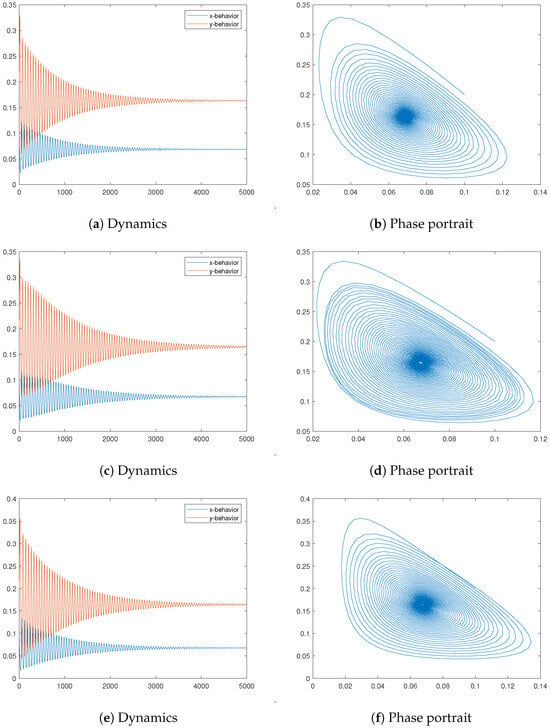
Figure 16. In the first column, dynamics of the considered models are presented. The second column is for the phase portraits. In the first row, we present model (18)—the normal distribution is used for the x-component and the gamma one for the y-component. For the second line, the gamma distribution is replaced by the exponential one. The third line is for model (22)—the normal and exponential distributions are used.

In the second line of Figure 16, we replace the gamma distribution for the y-dynamics with the exponential one. Its intensity is assumed to be relatively high, $\lambda =10$. Although there are some differences, we can see that the similarities are greater.

We generalize model (4) further. We can introduce a growing impact in the perturbations by multiplying each term by its number, i.e., the j-th term turns into $j{a}_{j}sin\left(j\omega t\right)$. Obviously, this is not essential in the discrete case since we may incorporate the multiplier j into the coefficient $a_j$. However, this is not the case for the model with a continuous perturbation defined by (10). For simplicity, we shall give only the x-dynamics:

$${\displaystyle \frac{\mathrm{d}x}{\mathrm{d}t}}=x\left(c-bx-2dy\right)+ϵ\left(l_{1}x+A_1\left(l_2+l_{3}x\right)\underset{\gamma \in \Omega }{\int }{\xi }_1\left(\gamma \right)sin\left({\xi }_1\left(\gamma \right)\omega t\right)\mathbb{P}\left(d\gamma \right)\right).$$

(19)

Hence, the periodic term can be transformed into

$$\begin{array}{cc}\hfill & \underset{\gamma \in \Omega }{\int }\xi \left(\gamma \right)sin\left(\xi \left(\gamma \right)\omega t\right)\mathbb{P}\left(d\gamma \right)=\underset{\gamma \in \Omega }{\int }\xi \left(\gamma \right){\displaystyle \frac{e^{i\xi \left(\gamma \right)\omega t}-e^{-i\xi \left(\gamma \right)\omega t}}{2i}}\mathbb{P}\left(d\gamma \right)\hfill \\ \hfill & =\mathbb{E}\left[\xi {\displaystyle \frac{e^{i\xi \omega t}-e^{-i\xi \omega t}}{2i}}\right]\hfill \\ \hfill & ={\displaystyle \frac{{\psi }^{\prime }\left(-\omega t\right)-{\psi }^{\prime }\left(\omega t\right)}{2}}.\hfill \end{array}$$

(20)

Using similar arguments as for deriving Equations (15)–(17), we obtain

$$\begin{array}{cc}\hfill & {\displaystyle \frac{{\Psi }_1^{\prime }\left(-x\right)-{\Psi }_1^{\prime }\left(x\right)}{2}}=e^{-{\displaystyle \frac{{\sigma }^2{x}^2}{2}}}\left(\mu sin\mu x+{\sigma }^{2}xcos\mu x\right),\hfill \\ \hfill & {\displaystyle \frac{{\Psi }_2^{\prime }\left(-x\right)-{\Psi }_2^{\prime }\left(x\right)}{2}}=\mathrm{sign}\left(x\right)\alpha \theta \sqrt{{\left(1+{\theta }^2{x}^2\right)}^{-\alpha -1}}sin\left(\left(\alpha +1\right)arccos\left({\displaystyle \frac{1}{\sqrt{1+{\theta }^2{x}^2}}}\right)\right),\hfill \\ \hfill & {\displaystyle \frac{{\Psi }_3^{\prime }\left(-x\right)-{\Psi }_3^{\prime }\left(x\right)}{2}}={\displaystyle \frac{2\lambda x}{{\left({\lambda }^2+x^2\right)}^2}}.\hfill \end{array}$$

(21)

For example, if we use the normal distribution for the x-dynamics and the exponential one for the y-part, we reach the following Lotka–Volterra-style model

$$\begin{array}{cc}\hfill {\displaystyle \frac{\mathrm{d}x}{\mathrm{d}t}}& =x\left(c-bx-2dy\right)+ϵ\left(l_{1}x+A_1\left(l_2+l_{3}x\right)\underset{\gamma \in \Omega }{\int }{\xi }_1\left(\gamma \right)sin\left({\xi }_1\left(\gamma \right)\omega t\right)\mathbb{P}\left(d\gamma \right)\right)\hfill \\ \hfill & =\left(c-bx-2dy\right)+ϵ\left(l_{1}x+A_1\left(l_2+l_{3}x\right){\displaystyle \frac{{\Psi }_1^{\prime }\left(-\omega t\right)-{\Psi }_1^{\prime }\left(\omega t\right)}{2}}\right)\hfill \\ \hfill & =x\left(c-bx-2dy\right)+ϵ\left(l_{1}x+A_1\left(l_2+l_{3}x\right)e^{-{\displaystyle \frac{{\sigma }^2{\omega }^2{t}^2}{2}}}\left(\mu sin\mu \omega t+{\sigma }^2\omega tcos\mu \omega t\right)\right),\hfill \\ \hfill {\displaystyle \frac{\mathrm{d}y}{\mathrm{d}t}}& =y\left(-c+2bx+dy\right)+ϵ\left(l_{1}y+A_2\left(l_2+l_{3}y\right){\displaystyle \frac{{\Psi }_3^{\prime }\left(-\omega t\right)-{\Psi }_3^{\prime }\left(\omega t\right)}{2}}\right)\hfill \\ \hfill & =y\left(-c+2bx+dy\right)+ϵ\left(l_{1}y+A_2\left(l_2+l_{3}y\right){\displaystyle \frac{2\lambda \omega t}{{\left({\lambda }^2+{\omega }^2{t}^2\right)}^2}}\right).\hfill \end{array}$$

(22)

The behavior of this model based on the same parameters can be viewed in the third line of Figure 16.

We can generalize further our model using higher powers in dynamics (19) using the relation

$$\mathbb{E}\left[{\xi }^n{e}^{i\xi x}\right]={\left(-i\right)}^n{\psi }^{\left(n\right)}\left(x\right).$$

(23)

Thus, we can transform the periodic term (20) into

$$\begin{array}{cc}\hfill & \underset{\gamma \in \Omega }{\int }{\left(\xi \left(\gamma \right)\right)}^{n}sin\left(\xi \left(\gamma \right)\omega t\right)\mathbb{P}\left(d\gamma \right)=\underset{\gamma \in \Omega }{\int }{\left(\xi \left(\gamma \right)\right)}^n{\displaystyle \frac{e^{i\xi \left(\gamma \right)\omega t}-e^{-i\xi \left(\gamma \right)\omega t}}{2i}}\mathbb{P}\left(d\gamma \right)\hfill \\ \hfill & =\mathbb{E}\left[{\xi }^n{\displaystyle \frac{e^{i\xi \omega t}-e^{-i\xi \omega t}}{2i}}\right]\hfill \\ \hfill & ={\left(-i\right)}^{n-1}{\displaystyle \frac{{\psi }^{\left(n\right)}\left(-\omega t\right)-{\psi }^{\left(n\right)}\left(\omega t\right)}{2}}.\hfill \end{array}$$

(24)

If we use the n-th power for the x-component and k-th power for the y-dynamics, then the Melnikov integral (12) turns into

$$M\left(t_0\right)={\int }_{-\infty }^{\infty }\left(\begin{array}{c}{\left(-i\right)}^{n-1}{A}_1{x}_0\left(t\right)\left(c-b{x}_0\left(t\right)-2d{y}_0\left(t\right)\right)\hfill \\ \times \left(l_1{y}_0\left(t\right)+\left(l_2+l_3{y}_0\left(t\right)\right){\displaystyle \frac{{\psi }_1^{\left(n\right)}\left(-\omega \left(t+t_0\right)\right)-{\psi }_1^{\left(n\right)}\left(\omega \left(t+t_0\right)\right)}{2}}\right)\hfill \\ +{\left(-i\right)}^{k-1}{A}_2{y}_0\left(t\right)\left(c-2b{x}_0\left(t\right)-d{y}_0\left(t\right)\right)\hfill \\ \times \left(l_1{x}_0\left(t\right)+\left(l_2+l_3{x}_0\left(t\right)\right){\displaystyle \frac{{\psi }_2^{\left(k\right)}\left(-\omega \left(t+t_0\right)\right)-{\psi }_2^{\left(k\right)}\left(\omega \left(t+t_0\right)\right)}{2}}\right)\hfill \end{array}\right)\mathrm{d}t.$$

(25)

Next, we modify three-dimensional model (7) involving such higher order powers. We have, for the exponential distribution,

$$\begin{array}{c}\hfill {\Psi }_3^{\left(n\right)}\left(x\right)={\displaystyle \frac{i^n\lambda }{{\left(\lambda -ix\right)}^{n+1}}}.\end{array}$$

(26)

For $n=2$, we obtain

$$\begin{array}{c}\hfill {\left(-i\right)}^{n-1}{\displaystyle \frac{{\Psi }_3^{\left(n\right)}\left(-x\right)-{\Psi }_3^{\left(n\right)}\left(x\right)}{2}}=\lambda x{\displaystyle \frac{3{\lambda }^2-x^2}{{\left({\lambda }^2+x^2\right)}^3}}.\end{array}$$

(27)

As an example, we consider a three-dimensional Lotka–Volterra model for which the first component is with a zero-powered Gaussian term, for the second component we use a first-powered Gamma term, and for the third component we apply the second power of the exponential distribution—formula (15), the second formula from (21), and formula (27), respectively. Thus, we reach the following model:

$$\begin{array}{cc}\hfill {\displaystyle \frac{\mathrm{d}x}{\mathrm{d}t}}& =x\left(c-bx-2dy+az\right)+ϵ\left(l_{1}x+A_1\left(l_2+l_{3}x\right)\underset{\gamma \in \Omega }{\int }sin\left({\xi }_1\left(\gamma \right)\omega t\right)\mathbb{P}\left(d\gamma \right)\right)\hfill \\ \hfill & =\left(c-bx-2dy\right)+ϵ\left(l_{1}x+A_1\left(l_2+l_{3}x\right){\displaystyle \frac{{\Psi }_1\left(\omega t\right)-{\Psi }_1\left(-\omega t\right)}{2i}}\right)\hfill \\ \hfill & =x\left(c-bx-2dy\right)+ϵ\left(l_{1}x+A_1\left(l_2+l_{3}x\right)e^{-{\displaystyle \frac{{\sigma }^2{\omega }^2{t}^2}{2}}}sin\mu \omega t\right),\hfill \\ \hfill {\displaystyle \frac{\mathrm{d}y}{\mathrm{d}t}}& =y\left(-c+2bx+dy-az\right)+ϵ\left(l_{1}y+A_2\left(l_2+l_{3}y\right)\underset{\gamma \in \Omega }{\int }{\xi }_2\left(\gamma \right)sin\left({\xi }_2\left(\gamma \right)\omega t\right)\mathbb{P}\left(d\gamma \right)\right)\hfill \\ \hfill & =y\left(-c+2bx+dy\right)+ϵ\left(l_{1}y+A_2\left(l_2+l_{3}y\right){\displaystyle \frac{{\Psi }_2^{\prime }\left(-\omega t\right)-{\Psi }_2^{\prime }\left(\omega t\right)}{2}}\right)\hfill \\ \hfill & =y\left(-c+2bx+dy\right)+ϵl_{1}y\hfill \\ \hfill & +ϵA_2\left(l_2+l_{3}y\right)\mathrm{sign}\left(\omega t\right)\alpha \theta \sqrt{{\left(1+{\theta }^2{\omega }^2{t}^2\right)}^{-\alpha -1}}sin\left(\left(\alpha +1\right)arccos\left({\displaystyle \frac{1}{\sqrt{1+{\theta }^2{\omega }^2{t}^2}}}\right)\right),\hfill \\ \hfill {\displaystyle \frac{\mathrm{d}z}{\mathrm{d}t}}& =ϵz\left(l_4-l_{6}x+l_{7}y-l_{8}z+l_5{A}_3\underset{\gamma \in \Omega }{\int }{\left({\xi }_3\left(\gamma \right)\right)}^{2}sin\left({\xi }_3\left(\gamma \right)\omega t\right)\mathbb{P}\left(d\gamma \right)\right)\hfill \\ \hfill & =ϵz\left(l_4-l_{6}x+l_{7}y-l_{8}z-i{l}_5{A}_3{\displaystyle \frac{{\Psi }_3^{\left(2\right)}\left(-\omega t\right)-{\Psi }_3^{\left(2\right)}\left(\omega t\right)}{2}}\right)\hfill \\ \hfill & =ϵz\left(l_4-l_{6}x+l_{7}y-l_{8}z+l_5{A}_3\lambda \omega t{\displaystyle \frac{3{\lambda }^2-{\omega }^2{t}^2}{{\left({\lambda }^2+{\omega }^2{t}^2\right)}^3}}\right).\hfill \end{array}$$

(28)

The behavior of this model can be seen in Figure 17. The values of the additional parameters used are $l_4=5.1$, $l_5=15.3$, $l_6=7.1$, $l_7=8.2$, $l_8=14.3$, $A_3=1$, and $z\left(0\right)=0.01$.

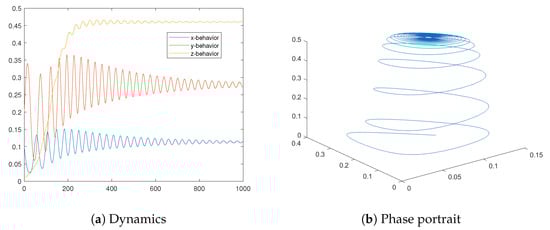
Figure 17. Dynamics of the three-dimensional model (28) are presented—we use the normal, gamma, and exponential distributions for the x-, y-, and z-components, respectively.

6. Concluding Remarks

In this article, we investigate the chaos of a generalized perturbed Lotka–Volterra model containing many free parameters (the coefficients $a_i;i=1,2,\dots ,N$).

Nonstandard methods for simultaneously solving all roots of generalized exponential and trigonometric equation of the type $M(t_0)=0$ can be found in [42].

Similar theoretical studies and simulations can be performed on a wide class of reaction kinetic models described in the literature (see, for example, [43]).

We anticipate future research on this fascinating topic in light of the concerns presented in this paper. This analysis will cover the computation of Lyapunov exponents, the creation of bifurcation diagrams, the application of Poincaré maps, clearing parameter ranges in the two-dimensional model, summarizing sufficient or necessary conditions for the occurrence of chaos, providing a more systematic discussion on the applicability conditions of the Melnikov criterion in the presence of multi-frequency perturbations, systematically discussing how the dynamical complexity evolves as the parameter N increases, and performing long-term trajectory simulations.

We also envisage research related to the validation of possible chaos in dynamical systems based on already developed and practically applied discrete chaotic neuron models. For more details, see the excellent article in [44].

Challenges for Learners

We provide an efficient study strategy that emphasizes learning and challenges our PhD students to consider the triangle of enigmatics, creativity, and acmeology.

After providing curriculum modules, we will set the following tasks for self-learning.

Task 1

(self-learning). Study the behavior of model (4) at fixed values: $N=7$, $c=0.6$, $b=0.5$, $d=0.4$, $l_1=-0.001$, $l_2=1$, $l_3=0.03$, $a_1=0.11$, $a_2=0.51$, $a_3=0.11$, $a_4=9.23$, $a_5=0.14$, $a_6=0.7$, $a_7=0.2$ for $x_0=0.1$, $y_0=0.3$:

(a) 

For what value of the parameter ϵ ($0<ϵ\le 1$) and ω is the phase portrait depicted in Figure 18 obtained?

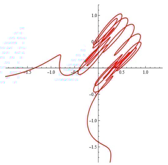Figure 18. Phase portrait (Task 1 (self-learning)).

(b) 

Show a chaotic phase portrait/sensitive dependence for parameters above this threshold.

(c) 

Draw the corresponding conclusions.

Task 2

(self-learning). Study the behavior of model (7) at fixed values: $N=8$, $c=b=d=a=0.5$, $l_1=-0.3$, $l_2=0.4$, $l_3=0.51$, $l_4=1.12$, $l_5=2.01$, $l_6=0.1$, $l_7=0.2$, $l_8=0.9$, $a_1=0.95$, $a_2=0.301$, $a_3=0.295$, $a_4=0.95$, $a_5=0.95$, $a_6=0.1$, $a_7=0.25$, $a_8=0.9$ for $x_0=0$, $y_0=0$, $z_0=0.002$:

(a) 

For what value of the parameter ϵ ($0<ϵ\le 1$) and ω is the phase portrait depicted in Figure 19d obtained?

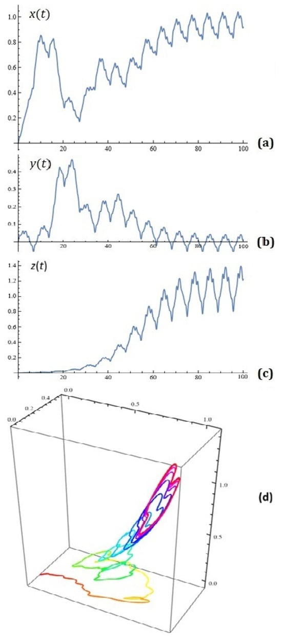Figure 19. (a) $x(t)$ component of the solution of system (7); (b) $y(t)$ component of the solution of system (7); (c) $z(t)$ component of the solution of system (7); (d) Phase portrait (Task 2 (self-learning)).

(b) 

Draw the corresponding conclusions.

Task 3

(self-learning with increased difficulty). Let $N=4$, $c=b=d=a=0.5$, $\omega =1.01$, $ϵ=0.15$:

(a) 

For what values of the remaining parameters of model (7) is the phase portrait depicted in Figure 20 obtained?

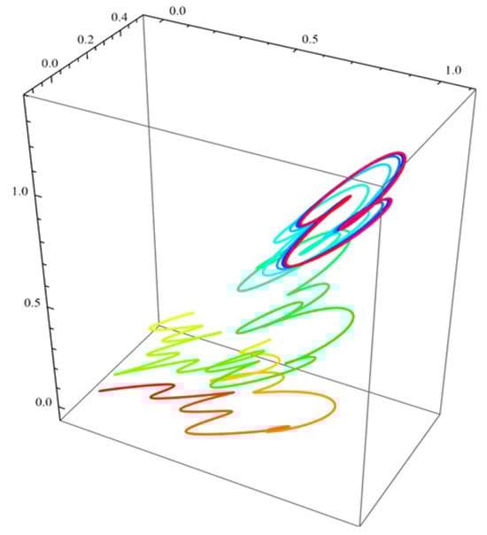Figure 20. Phase portrait (Task 3 (self-learning)).

(b) 

Draw the corresponding conclusions.

We would be very grateful to readers who can share their experience regarding the discussion we have opened, including methodological problems in teaching this specific subject.

Our conclusion as teachers is that with the proposed methodology, students adapt relatively well and touch upon the elegant theory of Andronov–Melnikov for the possible occurrence of chaos in the dynamical system under consideration.

References

- Lotka, A.J. Elements of Physical Biology; Williams and Wilkins: Baltimore, MD, USA, 1925. [Google Scholar]
- Volterra, V. Theorie Mathematique de la Lutte pour la Vie; Gauthier-Villars: Paris, France, 1931. [Google Scholar]
- Coste, J.; Peyraud, J.; Coullet, P. Asymptotic Behaviour in the Dynamics of Competing Species. SIAM J. Appl. Math. 1979, 36, 516–543. [Google Scholar] [CrossRef]
- Farkas, M. Periodic Motions; Springer: New York, NY, USA, 1994. [Google Scholar]
- Gilpin, M.E. Spiral Chaos in a Predator-Prey Model. Am. Nat. 1979, 113, 306–308. [Google Scholar] [CrossRef]
- Guckenheimer, J.; Holmes, P. Nonlinear Oscillations, Dynamical Systems, and Bifurcations of Vector Fields; Springer: New York, NY, USA, 1983. [Google Scholar]
- Hofbauer, J.; Schuster, P.; Sigmund, K.; Wolff, R. Dynamical Systems under Constant Organization II: Homogeneous Growth Functions of Degree p = 2. SIAM J. Appl. Math. 1980, 38, 282–304. [Google Scholar] [CrossRef]
- Hofbauer, J.; Sigmund, K. The Theory of Evolution and Dynamical Systems; Cambridge University Press: Cambridge, UK, 1988. [Google Scholar]
- Inoue, M.; Kamifukumoto, H. Scenarios Leading to Chaos in a Forced Lotka-Volterra Model. Prog. Theor. Phys. 1984, 71, 930–937. [Google Scholar] [CrossRef][Green Version]
- Kuznetsov, Y.A.; Muratori, S.; Rinaldi, S. Bifurcations and Chaos in a Periodic Predator-Prey Model. Int. J. Bifurc. Chaos 1992, 2, 117–128. [Google Scholar] [CrossRef]
- Li, J. Chaos and Melnikov’s Method; Chongqing University: Chongqing, China, 1989. (In Chinese) [Google Scholar]
- Melnikov, V.K. On the Stability of the Center for Time-Periodic Perturbations. Trans. Mosc. Math. Soc. 1963, 12, 3–52. [Google Scholar]
- Rinaldi, S.; Muratori, S.; Kuznetsov, Y.A. Multiple Attractors, Catastrophes and Chaos in Seasonally Perturbed Predator-Prey Communities. Bull. Math. Biol. 1993, 55, 15–35. [Google Scholar] [CrossRef]
- Sabin, G.C.W.; Summers, D. Chaos in a Periodically Forced Predator-Prey Ecosystem Model. Math. Biosci. 1993, 113, 91–113. [Google Scholar] [CrossRef] [PubMed]
- Schaffer, W.M. Order and Chaos in Ecological Systems. Ecology 1985, 66, 93–106. [Google Scholar] [CrossRef]
- May, R.; Leonard, W. Nonlinear Aspects of Competition Between Three Species. SIAM J. Appl. Math. 1975, 29, 243–253. [Google Scholar] [CrossRef]
- Schuster, P.; Sigmund, K.; Wolff, R. On α-Limits for Competition Between Three Species. SIAM J. Appl. Math. 1979, 37, 49–54. [Google Scholar] [CrossRef]
- Shaw, S.W.; Wiggins, S. Chaotic Dynamics of a Whirling Pendulum. Phys. D Nonlinear Phenom. 1988, 31, 190–211. [Google Scholar] [CrossRef]
- Shaw, S.W.; Wiggins, S. Chaotic Motions of a Torsional Vibration Absorber. J. Appl. Mech. 1988, 55, 952–958. [Google Scholar] [CrossRef]
- Ushiki, S. Central Difference Scheme and Chaos. Phys. D Nonlinear Phenom. 1982, 4, 407–424. [Google Scholar] [CrossRef]
- Ushiki, S.; Yamaguti, M.; Matano, H. Discrete Population Models and Chaos. In Lecture Notes in Numerical Applied Analysis; North-Holland Publishing Company: Amsterdam, The Netherlands, 1980; Volume 2, pp. 1–25. [Google Scholar]
- Wiggins, S. Global Bifurcations and Chaos: Analytical Methods; Springer: New York, NY, USA, 1988. [Google Scholar]
- Wiggins, S. Introduction to Applied Nonlinear Dynamical Systems and Chaos; Springer: New York, NY, USA, 1990. [Google Scholar]
- Wiggins, S. Chaotic Transport in Dynamical Systems; Springer: New York, NY, USA, 1992. [Google Scholar]
- Wiggins, S.; Holmes, P. Homoclinic Orbits in Slowly Varying Oscillators. SIAM J. Math. Anal. 1987, 18, 612–629. [Google Scholar] [CrossRef]
- Wiggins, S.; Holmes, P. Periodic Orbits in Slowly Varying Oscillators. SIAM J. Math. Anal. 1987, 18, 592–611. [Google Scholar] [CrossRef]
- Wiggins, S.; Shaw, S.W. Chaos and Three-Dimensional Horseshoes in Slowly Varying Oscillators. J. Appl. Mech. 1988, 55, 959–968. [Google Scholar] [CrossRef]
- Kyurkchiev, N.; Boyadjiev, G. Dynamics of Modified Lotka–Volterra Model with Polynomial Intervention Factors. Methodological Aspects. III. Int. J. Differ. Equ. Appl. 2021, 20, 121–132. [Google Scholar]
- Kyurkchiev, V.; Boyadjiev, G.; Kyurkchiev, N. A Software Tool for Simulating the Dynamics of a New Extended Family of Lotka–Volterra Competition Model. Int. J. Differ. Equ. Appl. 2022, 21, 33–46. [Google Scholar]
- Agarwal, R.; Hristova, S.; O’Regan, D. Non-Instantaneous Impulses in Differential Equations; Springer: Cham, Switzerland, 2017. [Google Scholar]
- Stamova, I.; Stamov, G. On the Uniform Stability of Impulse Lotka–Volterra Type Systems with Supremums. Biomath Commun. 2017, 4, 18. [Google Scholar]
- Leconte, M.; Masson, P.; Qi, L. Limit Cycle Oscillations, Response Time and the Time-Dependent Solution to the Lotka–Volterra Predator-Prey Model. Phys. Plasmas 2022, 29, 022109. [Google Scholar]
- Prasolov, A. Some Quantitative Methods and Models in Economic Theory. Economic Issues, Problems and Perspectives; Nova Science Publishers: New York, NY, USA, 2016. [Google Scholar]
- Orbach, Y. Forecasting the Dynamics of Market and Technology; Ariel University Press: Ariel, Israel, 2022. [Google Scholar]
- Unsal Ozdilek, I. Integrating Lotka-Volterra Dynamics and Gravity Modeling for Regional Population Forecasting. Front. Built Environ. 2025, 11, 1542946. [Google Scholar] [CrossRef]
- Vollert, S.A. Bayesian Model Calibration in Applied Mathematics: Incorporating Novel Information in Ecological Systems and Beyond. Ph.D. Thesis, Queensland University of Technology, Brisbane, Australia, 2025. [Google Scholar]
- Tauber, U.C. Stochastic Spatial Lotka-Volterra Predator-Prey Models. arXiv 2024, arXiv:2405.0500. [Google Scholar]
- Christie, J.R.; Gopalsamy, K.; Li, J. Chaos in Perturbed Lotka-Volterra Systems. ANZIAM J. 2001, 42, 399–412. [Google Scholar] [CrossRef][Green Version]
- Kyurkchiev, N.; Andreev, A. Approximation and Antenna and Filters Synthesis. Some Moduli in Programming Environment MATHEMATICA; LAP LAMBERT Academic Publishing: Saarbrücken, Germany, 2014. [Google Scholar]
- Kyurkchiev, N.; Zaevski, T.; Iliev, A.; Kyurkchiev, V.; Rahnev, A. Dynamics of a New Class of Extended Escape Oscillators: Melnikov’s Approach, Possible Application to Antenna Array Theory. Math. Inform. 2024, 67, 1–15. [Google Scholar] [CrossRef]
- Kyurkchiev, N.; Zaevski, T.; Iliev, A.; Kyurkchiev, V.; Rahnev, A. Studying Homoclinic Chaos in a Class of Piecewise Smooth Oscillators: Melnikov’s Approach, Symmetry Results, Simulations and Applications to Generating Antenna Factors Using Approximation and Optimization Techniques. Symmetry 2025, 17, 1144. [Google Scholar] [CrossRef]
- Makrelov, I.; Kyurkchiev, N.; Tamburov, S. Two Two-Sided Methods for Simultaneous Determination of All Roots of Trigonometric and Exponential Polynomials. Trav. Sci. Univ. Plovdiv Math. 1985, 23, 289–298. [Google Scholar]
- Murray, J.D. Mathematical Biology. I. An Introduction, 3rd ed.; Springer: Berlin/Heidelberg, Germany, 2001. [Google Scholar]
- Suo, G.; Zhang, Z.; Li, Q.; Ding, S.; Iu, H.H.C.; Cao, Y.; Xu, X.; Wang, C.; Mou, J. Encrypt a Story: A Video Segment Encryption Method Based on the Discrete Sinusoidal Memristive Rulkov Neuron. IEEE Trans. Dependable Secure Comput. 2025, 22, 8011–8024. [Google Scholar]
Disclaimer/Publisher’s Note: The statements, opinions and data contained in all publications are solely those of the individual author(s) and contributor(s) and not of MDPI and/or the editor(s). MDPI and/or the editor(s) disclaim responsibility for any injury to people or property resulting from any ideas, methods, instructions or products referred to in the content. |
© 2026 by the authors. Licensee MDPI, Basel, Switzerland. This article is an open access article distributed under the terms and conditions of the Creative Commons Attribution (CC BY) license.