A Chemistry-Based Optimization Algorithm for Quality of Service-Aware Multi-Cloud Service Compositions

Abstract

The increasing complexity of cloud service composition demands innovative approaches that can efficiently optimize both functional requirements and quality of service (QoS) parameters. While several methods exist, they struggle to simultaneously minimize the number of combined clouds, examined services, and execution time while maintaining a high QoS. This novelty of this paper is the chemistry-based approach (CA) that draws inspiration from the periodic table’s organizational principles and electron shell theory to systematically reduce the complexity associated with service composition. As chemical elements are organized in the periodic table and electrons organize themselves in atomic shells based on energy levels, the proposed approach organizes cloud services in hierarchical structures based on their cloud number, composition frequencies, cloud quality, and QoS levels. By mapping chemical principles to cloud service attributes—where service quality levels correspond to electron shells and service combinations mirror molecular bonds—an efficient framework for service composition is created that simultaneously addresses multiple objectives in QoS, NC, NEC, NES, and execution time. The experimental results demonstrated significant improvements over existing methods, such as Genetic Algorithms (GAs), Simulated Annealing (SA), and Tabu Search (TS), across multiple performance metrics, i.e., reductions of 14–33% are observed in combined clouds, while reductions of 20–85% are observed in examined clouds, and reductions of 74–98% are observed in examined services. Also, a reduction of 10–99% is observed in execution time, while fitness levels are enhanced by 1–14% compared to benchmarks. These results validate the proposed approach’s effectiveness in optimizing service composition while minimizing computational overhead in multi-cloud environments.

1. Introduction

The exponential growth in cloud service adoption has fundamentally transformed how user applications are deployed and accessed over the Internet [1,2,3,4]. This transformation has led to an unprecedented increase in the availability of online services [5,6,7], creating both opportunities and challenges in service composition and management. Cloud services exist in two primary forms—single services offering basic functionality and composite services that combine multiple primitives to meet complex requirements. While single services serve specific needs, they often fall short in addressing sophisticated user requirements, driving the demand for composite services [1,5].

Efficient service composition in multi-cloud environments (MCEs) presents several critical challenges. Service providers must optimize multiple competing objectives simultaneously, including QoS, execution time, and resource usage. The complexity of selecting optimal service combinations from vast service pools, coupled with the challenge of minimizing inter-cloud communication overhead, makes this task particularly demanding. Additionally, maintaining reliability while reducing the number of combined clouds poses a significant technical challenge that current solutions have yet to fully address.

Current approaches to service composition, particularly those employing nature-inspired algorithms (NIAs), have demonstrated success in solving difficult optimization problems [8,9,10,11,12]. However, significant limitations persist in existing solutions. Most current approaches focus on single-cloud environments [5,13], making them vulnerable to single points of failure. Multi-cloud approaches lack efficient mechanisms for simultaneously optimizing the number of combined clouds (NC) and quality of service (QoS). Furthermore, while previous studies [13,14,15,16,17] address NC optimization, they fail to balance it effectively with other critical parameters.

To address these limitations, an innovative chemistry-based approach (CA) is proposed that draws inspiration from the organizational principles of the periodic table and electron shell theory. The key innovations of the proposed work are outlined below.

The proposed approach establishes a novel mapping between chemical concepts and cloud service composition. The services are organized in hierarchical structures based on QoS levels, similar to how electrons organize themselves in shells based on energy levels. In addition, SFs (Service Files), which describe service tasks, are arranged in an SF table based on composition frequency and cloud distribution, mirroring the periodic table’s organization of elements according to atomic properties. The service composition and optimization methodology in this research approach are analogously modeled on the periodic table’s structure and the dynamic behavior of electrons transitioning between shells during chemical reactions.

The proposed approach uniquely structures SFs in a novel SF table that groups SFs according to their composition frequency and distribution across clouds. Within each SF, services are further arranged in four QoS levels (very high, high, medium, and low), mirroring electron shell organization in atoms. This organization significantly enhances the efficiency of service composition while maintaining high-quality standards. The innovation and novelty can be defined as follows:

Service File (SF) Table for Systematic Composition: This research work elaborated on organizing SFs (Service Files) in a tabular format that is based on the composition frequency and cloud distribution. It depicts the periodic table’s classification of elements according to their atomic number and number of shells to provide efficient SF selection.

Electron Transition-Inspired Optimization: The proposed work models service arrangement, which is based on the electron configuration according to energy level. This significantly enhances efficiency in selection by leveraging the principles of electron shell theory.

The main contributions of this research are as follows:

A Novel Chemistry-Inspired Approach (CA): This method uses the periodic table and electron shell theory to streamline service composition and help in moderating its inherent complexity.

A Multi-Objective Optimization Framework: The proposed framework balances competing objectives in a better way. These include QoS, NC, NEC, NES, and execution time.

Empirical Validation and Comparative Analysis: Experimental results demonstrate performance enhancements over the available optimization techniques. The techniques included are Genetic Algorithms (GAs), Simulated Annealing (SA), and Tabu Search (TS). The enhancements span across multiple key metrics.

The remainder of this paper is organized as follows: Section 2 discusses the state of the art in this field, Section 3 presents the problem statement, Section 4 explains the proposed CA methodology, Section 5 outlines the experimental design, Section 6 presents results and analysis, and Section 7 concludes with future research directions.

2. Related Work

This section reviews existing studies by classifying service composition algorithms into traditional, nature-inspired, and hybrid service composition methods. The following subsections delve into the details of these algorithms.

2.1. Traditional Service Composition Algorithms

A variety of traditional algorithms have been developed to address service composition problems. Cassar et al. [18] proposed a divide-and-conquer algorithm that breaks down composition requests into simpler sub-requests. This iterative process continues until each sub-request finds at least one service that satisfies its requirements, forming a composite service by combining the identified services. Some algorithms focus on meeting QoS requirements. For example, Shang et al. [19] proposed an approach for service composition using a bipartite-directed graph. Ghobaei-Arani and Souri [20] suggested an approach based on linear programming to select an efficient quality-oriented web service composition (QWSC) for every request in a cloud environment. Guidara et al. [21] developed exact and approximate approaches for small and large selection problems, respectively, incorporating a pruning technique to minimize the search space and enhance efficiency.

In MCEs, research on minimizing the NC for efficient service composition remains limited. Kurdi et al. [15] proposed a combinatorial optimization algorithm-based method. By choosing the cloud with the highest number of SFs, their approach increased the delivery of composite services with the smallest NC in the shortest period of time. Mezni et al. [22] presented a formal concept analysis-based service composition method for identifying and classifying cloud compositions while reducing the NC and communication overhead. Nazari et al. [23] introduced a tree-based similarity metric to select suitable clouds and composition plans to improve load balancing between multiple clouds. Yin and Hao [16] devised an energy-aware multi-target service composition method (EMTSC) to reduce energy usage, execution time, and NC by accounting for networks between users and clouds, as well as network connections between clouds. The cloud service provider count is considered a crucial parameter during the service composition process. In cloud computing environments, it directly affects response time, energy usage, and overall cost. Souri et al. [17] proposed a formal verification framework for ensuring service composition with a high QoS in an MCE by reducing the number of cloud service providers. Employing a multi-label transition system and algebra methods based on Pi calculus, this approach allows for an examination of service composition while considering both functional and non-functional features, such as QoS standards. Heidari and Emadi [5] developed a skyline service algorithm for modeling the relationship between cloud service providers and clouds by minimizing the NC, the providers, and the communication between them.

2.2. Nature-Inspired Service Composition Algorithms

NIAs mimic biological, physical, or chemical phenomena in nature [24] and are often employed to obtain optimized solutions for service composition problems [8]. NIAs can be classified into three main groups—chemistry-based, physics-based, and bio-based approaches [24]. The following subsections provide a detailed description of these algorithms.

2.2.1. Bio-Based Methods

Bio-based methods are divided into two categories—evolution-based methods and swarm-based methods.

Evolution-based methods are optimization algorithms that draw inspiration from biological evolution and natural selection processes. Genetic Algorithms (GAs) represent one of their most prominent examples. GAs are widely used NIAs for optimizing service composition. Their execution involves four primary steps [8,25]. The first step is an initialization process, which involves randomly generating individual solutions in the initial population, where each chromosome represents a composite service. The second stage is a fitness evaluation, which involves assessing the quality of each solution to satisfy user needs. The third step—selection—involves choosing individual solutions to reproduce new solutions for the next generation. The fourth step entails evolving new solutions using crossover and mutation operations over the selected individual solutions. These four steps are iterated until a termination criterion is met, yielding an optimal solution.

Various enhancements for QoS optimization have been proposed, e.g., Tang et al. [26] introduced a hybrid genetic process combining local optimization at the end of each generation and the initial population to improve the overall quality of solutions. Grati et al. [27] proposed a penalty-based GA considering user QoS and resource constraints, achieving scalability compared to integer programming, especially with more web services and resources. Wang et al. [28] designed a GA-based approach for identifying QoS-aware service composition solutions in a geographically distributed cloud environment. In addition, Jatoth et al. [29] developed a fitness-aware service composition approach for cloud environments. They incorporated a GA based on adaptive genotype evolution, resolving connection constraints and optimizing quality-related metrics. Sadeghiram [30] suggested a multi-objective distributed approach for web service composition (WSC) that employs a novel local search method using link dominance and a non-dominated sorting GA. Similarly, Wang et al. [31] proposed a hybrid strategy to improve the Strength Pareto Evolutionary Algorithm 2 (SPEA2) for multi-objective optimization problems. In another study, Wang et al. [32], developed an adaptive mutation technique to enhance the performance of the SPEA2 algorithm in multi-objective WSC.

Other researchers employed clustering techniques for service composition problems. García et al. [33] employed GAs for location-aware, scalable service composition, proposing various solutions, such as a local express approach, a GA utility solution, and a pure GA solution. These solutions evaluate services to select the top candidate, with approaches like “U” and “express” reducing population size. While utility-based approaches rely on clustering candidate providers to complete tasks, express techniques prioritize providers with the highest fitness for each service.

Sadeghiram et al. [34] introduced a GA designed to improve end-to-end QoS by considering communication costs and delays. Their approach generates the initial population using a K-means clustering algorithm. Zhang et al. [35] employed fuzzy multi-objective linear programming to develop a constraint satisfaction-based WSC method aimed at addressing vague QoS requirements.

Swarm-based methods are optimization algorithms inspired by collective behaviors in nature, particularly how groups of organisms work together. These methods have been widely applied to service composition problems, where the goal is to combine individual web services to effectively create more complex functionality. The main effective approaches include particle swarm optimization (PSO) [36,37,38], ant colony optimization (ACO) [13,39,40], the artificial bee colony approach (ABC) [41,42], the fruit fly optimization algorithm (FOA) [43,44], the shuffled frog leaping algorithm [45], and the cuckoo search algorithm (CSA) [14,46,47]. Due to space limitations, the following discuss details of only a few of the most efficient NIAs, i.e., PSO, ACO, and the CSA.

Particle swarm optimization (PSO) algorithms, as introduced by Kennedy and Eberhart in 1995, are inspired by the food-seeking behavior of animals like birds and fish. This method relies on the swarm’s intergroup teamwork to direct the search for an optimal solution. The first step is to randomly generate the initial population and velocity of particles. The velocity and location of each particle are then updated during each iteration by retaining information about the global highest position and local top position. This allows the population of particles to ultimately reach a better search area [48,49].

Amiri et al. [36] proposed PSO for QWSC, where particles are modeled as vectors representing candidate WSCs. The particles are responsible for finding suitable candidates to fill the empty slots of the predefined workflow. The acceleration coefficients used to update the particle velocity are calculated using the method of Clerk and Kennedy [50]. Furthermore, Balakrishnan et al. [38] developed “the middleware for future Internet,” in conjunction with a composite Service Selection module, to assist in selecting optimal composite services based on solution quality and user experience. Fuzzy membership functions are used to model reputation, availability, and reliability. PSO is employed to select an ideal service from a set of paths inside a directed acyclic graph based on QoS. Nazif et al. [51] also created a fuzzy-based PSO algorithm for the creation of cloud composite services. To enhance the optimization process, their technique employs fuzzy membership rules and functions. In a similar vein, Tabalvandani et al. [52] proposed the use of a multi-objective PSO algorithm to create a cost-efficient and reliability-aware model for service composition in multi-cloud scenarios. Subsequently, Gao et al. [37] implemented an improved PSO (IPSO) method to compose services in a dynamic hybrid network. Initially, each service is categorized according to user requirements through interface matching. Following this, the IPSO algorithm generates a composition plan. If the fitness value of a service falls below a predefined threshold, it is substituted using a greedy algorithm. Conversely, if the overall composition fitness is below the threshold, the IPSO algorithm is reapplied to refine the composition.

Ant colony optimization (ACO) algorithms are a nature-inspired optimization technique that simulates the behavior of ants foraging toward the nearest food source. This mechanism is based on the pheromones deposited by ants, which guide others to follow the path, with a high pheromone intensity tied to the closest food source. Ants begin searching by randomly leaving their nest, and each ant lays pheromones in its track. The rate of evaporation and quality of paths are used to update the pheromone amounts. In subsequent iterations, the ants follow the path with the highest pheromone intensity, allowing them to converge toward a close-optimal solution [13,40,53,54].

Several researchers have developed algorithms to generate composite services in the shortest time. For instance, Yu et al. [13] proposed ACO-WSC and greedy–WSC to perform WSC in an MCE. Greedy–WSC selects the cloud providing the greatest number of required services and continues this process until all requirements are met. In ACO-WSC, each ant selects a random node in the graph and then searches for the next node based on pheromone and heuristic information on the connected edges to obtain optimal cloud combinations.

Alayed et al. [40] presented a novel ACO algorithm that increases convergence speed while avoiding premature convergence by utilizing the swap concept. To increase the chance for exploration, a multi-pheromone ACO was used, where each pheromone represents a single QoS value. Dahan [39] suggested a multi-agent system (MAS) using an ACO algorithm to identify a suitable candidate service matching user requirements. MAS utilizes different agents to quickly perform a distributed search.

The cuckoo search algorithm (CSA) is a novel evolutionary algorithm inspired by the parasitic behavior of cuckoo species, which lay their eggs in the nests of other birds. The CSA involves searching for nests with eggs that resemble the cuckoo’s own. The cuckoo locates the ideal nest and lays its eggs there without being detected by the nest owner. If the nest owner or host bird identifies the cuckoo’s eggs, it will discard them [55].

Wang et al. [47] introduced a two-phase method to combine credible services based on QoS. In the first phase, the service providers’ ability to provide the requested services is evaluated. In the subsequent phase, a modified CSA is applied to perform multi-objective service composition. Kurdi et al. [14] introduced the problem-dependent multi-cuckoo algorithm, which maintains a list of previously combined services. To reduce computation time, this approach uses a similarity algorithm to compare user requests with the list, ensuring user demands are met without examining many clouds. Ghobaei-Arani et al. [46] suggested a CSA that considers both service and network QoS for service composition in geo-distributed cloud systems.

2.2.2. Physics-Based Methods

SA is a physics-based approach for solving service composition problems that mimic the annealing process in metals [56]. Liu et al. [57] modeled a long-term quality-oriented service-based composition problem as an optimization problem, using metaheuristic methods like GAs, SA, and TS to find solutions. Deng et al. [58] presented an SA algorithm that minimizes energy consumption and risks to achieve an optimal mobile service composition. This approach accounts for the mobility of both service providers and requesters to reduce the risk of failure. Niewiadomski et al. [59] proposed two methods using generalized extreme optimization and SA techniques to solve the service composition problem. Each algorithm generates an initial population by exploiting a satisfiability modulo theory (SMT)-based procedure. To create an optimal composition service, the algorithms apply either SA or GEO to the initial population.

2.2.3. Chemistry-Based Methods

In recent years, several chemistry-inspired techniques have been introduced to enable distributed and efficient dynamic service composition. These methods, inspired by concepts such as chemical reactions, provide a flexible and adaptable means of combining services within a dynamic MCE [60,61]. Banatre et al. [60,61] proposed a framework for efficient service composition centered around chemistry-inspired techniques, including a chemical metaphor in which services combine and interact dynamically, akin to reactive chemical substances. Likewise, Di Napoli et al. [62] developed a chemical reaction model to dynamically address workflow requirements.

Viroli and Casadei [63] developed a coordination model for chemical reaction-based self-organizing structures called biochemical tuple spaces. Furthermore, Fernández et al. [64] created a chemistry-inspired workflow management system, emphasizing the decentralization of composite web service execution. Wang and Pazat [65] created chemistry-inspired middleware to enable self-adapting service composition. Additionally, Angelis et al. [66] applied a chemical-model approach to pervasive systems, using distributed data-sharing spaces for real-time, adaptive service compositions that respond dynamically to service addition and removal.

2.3. Hybrid Methods

Several researchers have attempted to address the limitations of individual algorithms by leveraging the advantages of other algorithmic features. Ko et al. [67] proposed an efficient hybrid QWSC method integrating SA and TS for constructing and running service composition systems in mobile cloud environments. Their algorithm ensures constraint-compliant service composition plans while minimizing search times and fulfilling clients’ QoS requirements. Spezzano [68] introduced a multi-objective PSO approach based on the crowding distance technique (MOPSO-CD) that selects a service while considering the dynamic characteristics of QoS during runtime. This approach solves the QoS-aware dynamic service selection problem using two different algorithms. MOPSO-CD is used to traverse the topology and find the best candidates for composite services, while the ant-based clustering technique is used to create and manage a service pool to lower the problem’s size by grouping services with equivalent functionality. This approach is highly scalable for large-scale problems.

Seghir and Khababa [44] proposed a hybrid algorithm combining GAs and the FOA to solve QoS-aware service composition problems. GAs employ an innovative roulette wheel for efficiency, while the FOA provides local search capabilities, balancing exploration and exploitation. Khanam et al. [69] introduced a hybrid approach combining ABC and PSO to prevent PSO from converging prematurely and to decrease the laborious updating of data in ABC to enable large-scale service composition. Similarly, Bhushan et al. [48] suggested a hybrid PSO (HPSO) coupled with FOA to prevent PSO for QoS-based service composition in cloud environments from converging prematurely. This strategy employs Pareto optimal solutions to increase the HPSO method’s rate of convergence. The PSO searches globally for an optimum solution, while the FOA conducts local searches that reduce computing time and speed up convergence, respectively.

Other significant contributions include hybrid approaches such as Sefati and Halunga’s [70] method, which combines GAs and ABC algorithms to enhance QoS-based cloud service composition. Using this approach, GAs initially select services that are then further refined by the ABC algorithm to satisfy customer needs. Dahan and Alwabel [71] integrated the ABC and CSA for service composition. Their approach enhances the performance of weaker bees using cuckoo agents. While ABC is efficient, it suffers from premature convergence issues—a limitation that is mitigated by the inclusion of the CSA. Bei et al. [72] employed a multi-pheromone technique with GA mutations to improve the ACO approach for QoS-aware multi-cloud service composition, minimizing the risk of local optima. Jayaudhaya et al. [73] combined GAs and the ACO algorithm to create a hybrid algorithm for efficient service composition in an MCE. They reported a significant improvement over traditional GAs and ACO methods due to the use of adaptive parameter tuning, where GAs dynamically adjust ACO parameters to improve flexibility and responsiveness to meet QoS requirements. Arasteh et al. [74] proposed a QoS-aware approach using an improved ant lion optimization algorithm to select optimal services from a pool of pre-existing services.

In recent years, cloud migration and multi-cloud service composition have emerged as critical decision-making areas due to their significant impact on operational efficiency, quality of service (QoS), and economic viability. Hosseini Shirvani et al. [75] proposed a comprehensive hybrid decision framework for cloud migration, integrating Analytic Hierarchy Process (AHP) and Delphi methodologies. Their framework systematically evaluates functional and non-functional requirements, economic considerations such as total cost of ownership (TCO), and sustainability factors to support robust cloud adoption decisions. This approach highlights the need for multi-dimensional decision-making criteria in managing complex cloud environments.

2.4. Discussions

The reviewed literature indicates that most existing methods focus on reducing the NC [5,13,14,15,22,23] while often neglecting QoS features. Furthermore, the performance of many approaches, aside from those of Kurdi et al. [14] and Mezni et al. [22], has been validated using small datasets. Table 1 provides a comparative analysis of service composition methods, in terms of the minimum NC, minimum NES, and QoS features. The summarized comparison is provided in Table 2. To the best of our knowledge, no prior research has comprehensively addressed the dual objectives of QoS functionality and the reduced NC. Therefore, there remains a critical need for algorithms that minimize the number of combined and examined clouds and services while maximizing solution quality. Although NIAs have shown promise in solving service composition problems, they suffer from limitations such as slow solution convergence and susceptibility to local optima. This underscores the need for novel approaches that provide faster service solutions and avoid local optima traps.

Table 1. Comparative analysis of service composition methods.

Reference	Minimum NC	Minimum NES	QoS Support
[15]	✓	✓	✗
[13,14,22,23]	✓	✗	✗
[16]	✓	✗	✓
[17]	✓ Min number of combined cloud providers	✗	✓
[5]	✓ Min NC and combined cloud providers	✗	✗
[18,59,60,63,64,66]	✗	✗	✗
[19,20,21,26,27,28,29,30,31,32,33,34,35,36,37,38,39,40,44,46,47,48,51,52,57,58,61,62,65,67,68,69,70,71,72,73,74,76]	✗	✗	✓
Proposed algorithm	✓	✓	✓

Note: ✓ = Supported, ✗ = Not supported.

Table 2. Summary table of service composition methods.

Performance Metrics	Number of References	Percentage (%)
Minimum NC	9	17%
Minimum NES	2	4%
QoS Support	41	77%
All Metrics	1	2%

While chemistry-based algorithms have shown remarkable success in diverse optimization problems, from healthcare resource allocation [77] to neural network training [78], their application in service composition remains largely unexplored [60,61,62,63,64,65,66]. These algorithms excel at handling complex, multi-constraint problems by mimicking chemical processes such as molecular interactions and electron shell transitions. Their proven effectiveness in solving related combinatorial challenges, particularly in association rule mining [79] and quadratic assignment problems [78], suggests significant potential for addressing the unique challenges of service composition. However, existing approaches have not fully leveraged chemical principles for optimizing multi-cloud service composition, especially in minimizing combined clouds while maintaining QoS requirements. This research bridges this gap by developing a novel chemistry-based algorithm that specifically targets the combinatorial complexity of service composition through the systematic organization and interaction patterns found in chemical systems.

3. Problem Statement

3.1. Preliminaries

Cloud services are arranged in a hierarchical structure, as defined in [15], consisting of multiple clouds (Cs), where C = {C1, C2, …, Cc}. Each cloud contains a collection of SFs, where SF = {SF1, SF2, …, SFf}. Each SF contains a set of services (Ss), where S = {S1, S2, …, Ss}.

SFs (also known as abstract services) are a description of service tasks. Ss (also known as concrete services) are a subset of SFs that perform similar tasks but with different QoS features [25].

3.2. Indicators

The indicators are NC, NEC, and NES.

To define SC formally, it is supposed that a user request contains n tasks {t1, t2, …, tn}. The SC algorithm locates and combines n available services from c clouds and f SFs to find an optimal solution denoted as {S1,1,13, S3,2,1, …, Sc,f,n}, where each Sc,f,n represents a specific service n selected from cloud c and SFf. The main objective of the SC algorithm is to minimize NC, NEC, and NES of the SC problem and maximize the quality of a solution (Q), as per Equation (1)

Min (NC, NEC, NES) And Max (Q)

(1)

4. System Design

This section introduces the CA, which is inspired by the principles of electron movement and the periodic table. Section 4.1 provides the chemical background underlying the CA method. Section 4.2 outlines the design of the CA. Section 4.3 explains the SF table, which arranges SFs based on their composition frequency and the total number of clouds. Section 4.4 describes the service table, which ranks services based on their quality. Section 4.5 details the process for searching the SF table to find a required SF. Finally, Section 4.6 describes the computational complexity of the system.

4.1. Chemistry Inspiration

The CA draws inspiration from the periodic table and the movement of electrons, highlighting similarities between foundational chemistry principles and the design of the CA. The key innovation of this proposed approach lies in its unique mapping between chemical concepts and cloud service composition. By organizing SFs in a periodic table-like structure based on composition frequency and establishing quality levels analogous to electron shells, an original framework is created that significantly reduces the search space while maintaining solution quality. This represents a fundamental departure from traditional metaheuristic approaches, introducing a new paradigm in cloud service composition.

4.1.1. Periodic Table

Since Mendeleev’s first periodic table in 1869, this organizational tool has driven the discovery and study of elements and materials [80]. Figure 1a depicts the current structure of the periodic table, which arranges and organizes chemical elements in order of increasing atomic numbers vertically and horizontally. As per Figure 1b, each cell contains the following important information [81,82]:

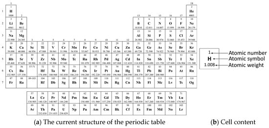
Figure 1. Periodic table [83].

• Atomic number: The number of protons in an atom, which determines the element and its chemical behavior.
• Atomic symbol: An abbreviation for an element (e.g., “C” for carbon).
• Atomic weight: The average mass of an element.

Periodic table columns are commonly referred to as groups. The valence electrons, or electrons in the outermost shell of an element, are identical for every element in the same column. Hence, they react in the same ways physically and chemically. For example, Group 18 elements are all inert gases with eight valence electrons. Each row is called a period, and the period number refers to the number of electron shells. For example, hydrogen is in the first row and contains only one electron shell [81].

4.1.2. Electron Movements Among Shells

Every element is composed entirely of a single kind of atom. Atoms consist of a nucleus, including protons and neutrons, and an outer region where electrons move in shells around the nucleus. According to the Bohr model, electrons can only be located in defined shells, each with a distinct energy level. Electrons closest to the nucleus have the lowest energy, while those further away have higher energy levels. Electrons can jump from one allowed shell to another by absorbing or emitting photons equal to the difference between the levels. An electron vanishes from the shell in which it is positioned and emerges again without ever being anywhere in between. Electrons absorb energy and jump to higher energy states [81]. Figure 2 depicts an electron jumping from shell n = 4 to shell n = 1, resulting in a photon perceived as red light.

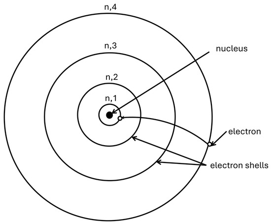
Figure 2. Bohr model [81].

4.1.3. Analogies Between Chemistry and Chemistry Algorithms

The fundamental principles of the periodic table and electron motion inspired this work. Similarly to how the periodic table groups elements based on atomic numbers, the proposed research organizes SFs in a table in reverse sequence based on their composition frequency. The SFs are arranged in rows according to the number of clouds containing them, analogous to the periodic table’s row-based arrangement of elements based on the number of electron shells. Frequently combined SFs are grouped in the same column, akin to the periodic table’s vertical grouping of elements with similar characteristics.

Services within a specific cloud and SF are grouped in a service table according to their QoS levels (very high, high, medium, and low). This arrangement mirrors the distribution of electrons according to their energy levels. Table 3 provides a mapping between components of the CA and the principles of the periodic table and electron movement.

Table 3. Mapping of CA components to the periodic table and electron movement.

CA	Periodic Table and Electrons
SF	Chemical elements
Composition frequency	Atomic number
Cloud number	Number of shells
QoS level	Energy level

4.2. System Architecture

Figure 3 illustrates the system architecture, which comprises the following key components:

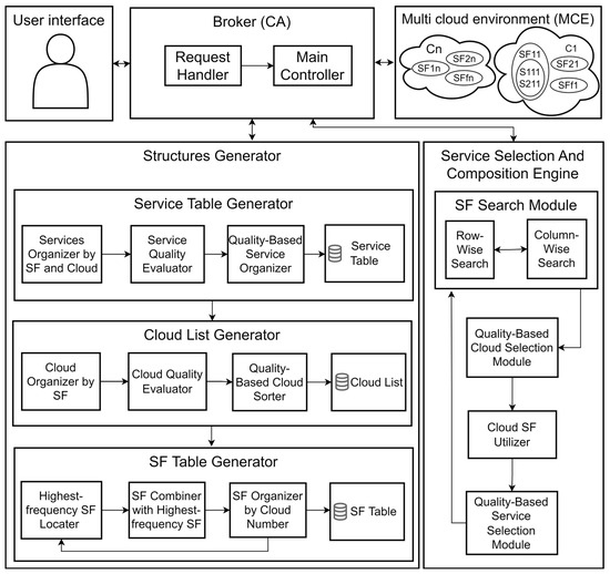
Figure 3. System architecture.

• Cloud services are arranged in an MCE [15], consisting of multiple clouds (Cs), where C = {C1, C2, …, Cc}. Each cloud contains a collection of SFs, where SF = {SF1, SF2, …, SFf}. Each SF comprises a set of services (Ss), where S = {S1, S2, …, Ss}.
• The user interface facilitates the submission of user requests and the presentation of the resulting composite service. This functionality is managed by the Request Handler and the Main Controller. The Main Controller plays a pivotal role in coordinating the operations of the Structure Generator and the Service Selection and Composition Engine. Specifically, it is responsible for transmitting the outputs produced by the Structure Generator, such as the SF table, to the Composition Engine, while also ensuring the efficient processing of requests received from the Request Handler.
• The CA, particularly the Structure Generator, is responsible for generating an SF table and a service table in cases where these tables have not been previously established, as explained in Section 4.3 and Section 4.4.
• The Cloud List, a subcomponent of the Structure Generator, employs the Cloud Organizer to classify clouds based on SF, as illustrated in Figure 4. Each SF maintains a systematically organized list of clouds in descending order of cloud quality. Each entry in the list is represented as C<Cloud number>,<Quality>, where the first value denotes the Cloud identifier and the second represents the associated Quality score. For instance, C1,6 corresponds to Cloud 1 with a Quality rating of 6. The sorting of clouds by quality is performed by the Quality-Based Cloud Sorter, with cloud quality being assessed based on two factors—the number of SFs (Nb_SFs) associated with the cloud and the number of services present in the first three columns of the service table (QoS_1, QoS_2, and QoS_3), which correspond to very high, high, and medium quality levels, respectively. It is computed using Equation (2).
  

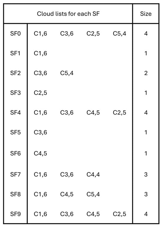  Figure 4. Cloud lists (Each entry, such as C1,6, represents a Cloud (Cloud Number, Quality).

$$Cloud Quality=0.3(Nb\_SFs)+0.4(QoS\_1)+0.2(QoS\_2)+0.1(QoS\_3)$$

(2)

Here, weights assigned to the number of SFs and the number of services in each corresponding column are represented by the numerical values of the coefficients 0.3, 0.4, 0.2, and 0.1. Poor-quality services (QoS_4) are excluded. The computation process is entirely carried out by the Cloud Quality Evaluator.

5.

As explained in Section 4.5, the CA searches the SF table for the requested SF using Service Selection and Composition Engine.

6.

Upon the selection of an SF, it is added to the composite list alongside the first cloud from its associated cloud list and the first service from the first column of the service table. If no service is available in the first column, the algorithm sequentially examines subsequent columns until a suitable service is identified. This selection process is governed by the Quality-Based Cloud Selection Module and the Quality-Based Service Selection Module, respectively. Once a service is integrated into a composite service, along with its associated cloud and SF, it is marked as unavailable for future compositions and is subsequently removed from the service table. The removal of a service can influence the associated cloud’s quality or its availability within the SF’s cloud list. Each removal prompts an update to the cloud’s quality, which may alter its ranking in the SF’s cloud list. If the removed service is the last available entry in the service table for a particular cloud, the cloud may also be removed from the SF’s cloud list as it can no longer provide the required SF. This, in turn, leads to an update in the SF table, where the row index of the affected SF is reduced by one, reflecting the cloud’s inability to support the SF.

7.

Subsequently, the CA utilizes the selected cloud for other SFs. Following all the steps laid out in point 6, the entire process is carried out again to select a service, after identifying a suitable SF. This iterative process continues until all requested SFs are sought within the selected cloud. This task is performed by the Cloud SF Utilizer.

8.

Steps 5, 6, and 7 are re-iterated until all requested SFs are incorporated into the composite service.

The pseudocode of the CA algorithm is presented in Algorithm 1, and its corresponding block diagram is illustrated in Figure 5. The main workflow of the system and the sequential stages involved in request processing are shown in Figure 6 and Figure 7, respectively.

Algorithm 1: Pseudocode of the CA Algorithm

Input: Clouds, SFs, Services   Output: Composite service INITIALIZATION:   1: If (SF Table = ∅)   2: Create Service table, Cloud lists, SF table, and Frequency Matrix   3: Number of Requests = 0 RECEIVE REQUESTS:   4: Request = New User Request   5: Number of Requests++ Locate SFs in SF TABLE:   6: Locate SFi from Remaining Requested SFs from SF Table   7: Locate Ci from SFi’s Cloud List LOCATE SERVICE:   8: Locate Si from Service table of SFi & Ci   9: Add (Ci, SFi, Si) to composite service   10: If (Is the Service Table of SFi & Ci Empty?)   11: Remove Ci from the SFi’s Cloud list   12: Reposition SF in the SF Table by decrementing its Row Index   13: If (Is the Service Table of SFi & Ci not empty?)   14: Update Ci Quality Due to Service Unavailability   15: Rearrange Clouds in the SFi’s Cloud list   16: If (Is Request not fulfilled)   17: SFi = Locate Remaining Requested SFs in Ci   18: If (SFi= ∅)   19: Go to Locate SFs in SF TABLE   20: If (SFi<> ∅)   21: Go to LOCATE SERVICE   22: If (Is Request fulfilled)   23: Update Frequency Matrix   24: Send the composite service to the user   25: If (Number of Requests= Max)   26: Update SF Table   27: Go to RECEIVE REQUESTS

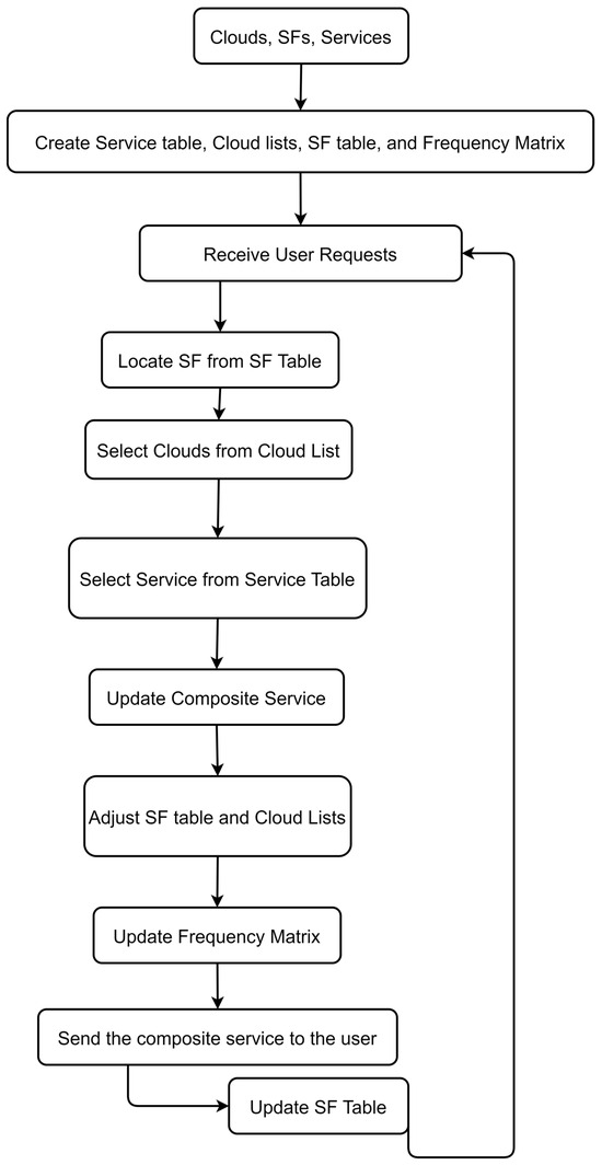
Figure 5. Block diagram illustrating the CA algorithm.

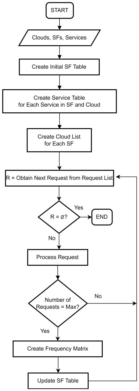
Figure 6. Main control algorithm.

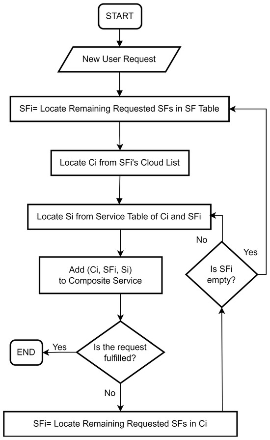
Figure 7. Request processing flow.

4.3. Generating the Service File Table

The SF table organizes SFs based on their composition frequency and the number of clouds, as depicted in Figure 8. SFs in the SF table are denoted as SFf,y, where f denotes the SF number and y represents the composition frequency, i.e., the number of times the SF is requested.

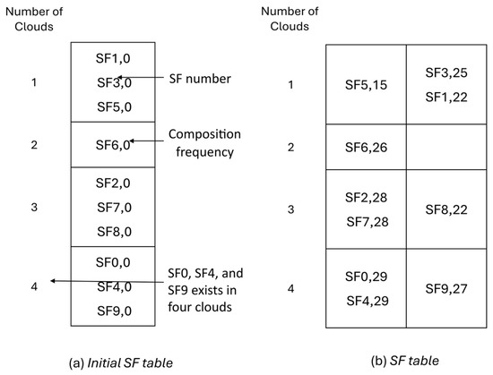
Figure 8. SF table (Each entry, such as SF1,22, represents a SF (SF Number, Composition Frequency).

Each column in the SF table groups SFs that are frequently requested together, while rows represent SFs associated with a specific number of clouds. For example, the first row lists SFs that are available in a single cloud. Within each cell of the SF table, SFs are arranged in reverse order based on their composition frequency.

In this research, it is suggested that the number of rows should be determined according to the maximum size of each SF cloud list. In contrast, the number of SFs (NSF) and the desired number of SFs per column (DSF) are used in Equation (3) to determine the number of columns in the SF table. For example, when NSF = 10 and DSF = 5, the table has two columns (10/5 = 2). The number of columns is set to one to generate the initial SF table, as depicted in Figure 8a. Each SF is placed in the correct row based on the number of clouds in which it exists. This task is performed by the SF Organizer. For example, SF1 and SF2 exist in one and three clouds, respectively, and so they are placed in rows 1 and 3. The number of columns required in the SF table is calculated using the following formula:

$$Number of Columns=\lceil {\displaystyle \frac{NSF}{DSF}}\rceil$$

(3)

Once the CA generates a maximum number of composite services (assumed to be 30 in this example) using its initial SF table searching process, a frequency matrix is generated to create an updated SF table, as depicted in Figure 8b. This matrix indicates how often SFs are requested with other SFs (Table 4). For example, SF1 is present in 22 out of 30 composite services, whereas it is only composed with SF0 14 times.

Table 4. Frequency matrix.

	SF0	SF1	SF2	SF3	SF4	SF5	SF6	SF7	SF8	SF9
SF0	29	14	28	12	29	15	25	28	17	18
SF1	0	22	14	5	14	5	13	14	8	22
SF2	0	0	28	12	28	15	25	28	17	25
SF3	0	0	0	25	12	8	12	12	12	25
SF4	0	0	0	0	29	15	25	28	17	26
SF5	0	0	0	0	0	15	13	15	10	13
SF6	0	0	0	0	0	0	26	25	17	26
SF7	0	0	0	0	0	0	0	28	17	25
SF8	0	0	0	0	0	0	0	0	22	22
SF9	0	0	0	0	0	0	0	0	0	27

The CA is initiated by identifying the SF with the highest frequency through the frequency matrix, utilizing the Highest-Frequency SF Locator. Subsequently, the SF table is updated to incorporate this SF along with additional SFs that collectively meet the specified frequency threshold, as determined by the SF Combiner. The new entries are placed in the first column of the SF table, distributed across rows based on the number of clouds. This process is repeated until all SFs are added to the SF table. Any SFs that do not fit into a column are compared against the highest-frequency SF in each column and assigned to the column where they have the greatest frequency. The frequency threshold is calculated using Equation (4), with a co-occurrence threshold of 70% assumed in this research, representing the percentage at which an SF co-occurs with the highest frequency SF.

$$Frequency threshold=Number of requests\ast Co-occurance Threshold$$

(4)

For instance, the algorithm updates column 1 with SF0 (the highest-frequency SF) and other SFs from the same row that meet the threshold frequency of 21 or higher. It only considers the first highest-frequency SF. Thus, SF4 was not selected despite its value being the same as that of SF0. SF9, with the next highest frequency, is placed in the second column along with corresponding SFs. The remaining SFs, such as SF5 with a frequency of 15 (below the threshold), are compared to the highest-frequency SFs in the existing columns and are assigned accordingly. In this case, the proposed algorithm compares the frequency of SF5 with that of SF0 and SF9, resulting in its addition to column 1 due to its higher frequency.

4.4. Generating the Service Table

A service table was created to display services and their QoS levels, as shown in Table 5. The focus here is on the four most important QoS features: two positive QoS features (reliability and availability) and two negative QoS features (cost and response time). Higher values indicate decreasing quality, whereas lower values indicate greater quality for negative features. Conversely, for positive features, higher values indicate higher quality, while lower values indicate worse quality [28,39,46].

Table 5. QoS parameters.

QoS Criterion	Unit	Description
Response time (T)	Millisecond	The amount of time elapsed between the task request and service assignment [46]
Availability (A)	Percent	The probability that services are available anytime and anywhere according to the user request [46]
Cost (C)	Dollar	Amount of money taken from the user to fulfill a request [46]
Reliability (R)	Percent	The percentage of tasks completed in comparison to tasks accepted [46]

The service table leverages these QoS metrics to refine service selection and optimization, ensuring that only those services that fulfill the best performance criteria are considered. It mainly focuses on the four most significant features of cloud services [8]. Availability (A) and reliability (R) represent the likelihood that a service is accessible and performs its tasks successfully. Cost (C) and response time (T) affect monetary expense and user experience. These four QoS features ensure that the system is dependable (accessible and correct), practical, and usable (affordability and speed).

Each SF within a given cloud is associated with a service table, which is managed by the Service Organizer. Columns represent QoS level types—very high (QoS_1), high (QoS_2), medium (QoS_3), and low (QoS_4)—spanning the value ranges 0.9–1, 0.79–0.89, 0.69–0.78, and 0–0.68, respectively, as depicted in Figure 9. Services are organized in columns within the service table according to their quality—a process that is executed by the Quality-Based Service Organizer. For instance, the service with the highest quality is positioned in the first column, surpassing the other services in that column.

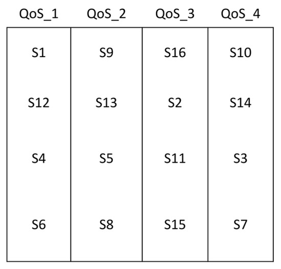
Figure 9. Service table.

Service quality was assessed by summing the QoS metrics, as outlined in Equation (5). This computation is carried out by the Service Quality Evaluator. This approach differs from previous methods [84,85], which calculate service quality by dividing the total positive QoS aspects (e.g., reliability and availability) by the total of negative QoS aspects (e.g., cost and time). These approaches emphasize the importance of decreasing negative QoS values and increasing positive QoS values. Based on several experiments, the division approach sometimes misinterprets service quality, particularly when QoS values are close to extremes (e.g., either 1 or 0.1). The proposed modification provides more accurate results by maximizing service quality.

$$Q\left(s\right)=w_{A }{\cdot NA+w}_R{ \cdot NR+w}_{T }{\cdot NT+w}_{C }\cdot NC$$

(5)

Here, $w_A{,w}_R{,w}_T{,w}_C$ and $NA,NR,NT,andNC$ represent the assigned weights and normalized QoS values of A, R, T, and C. The sum of all weights typically equals 1. The QoS values are normalized to a uniform scale of values between 0 and 1. Negative and positive QoS parameters are computed using Equations (6) and (7), respectively.

$$N{Q}^{-}={\displaystyle \frac{S{Q}^{-}-Q}{S{Q}^{+}-S{Q}^{-}}}$$

(6)

$$\mathrm{N}{\mathrm{Q}}^{+}={\displaystyle \frac{\mathrm{Q}-\mathrm{S}{\mathrm{Q}}^{+}}{\mathrm{S}{\mathrm{Q}}^{+}-\mathrm{S}{\mathrm{Q}}^{-}}}$$

(7)

Here, Q stands for the QoS parameter, while NQ⁻ and NQ⁺ are the normalized values of the negative and positive QoS service parameters, respectively. Furthermore, SQ⁻ and SQ⁺ denote the highest and lowest values of the QoS parameters [46]. Each QoS parameter is assigned a distinct weight value to emphasize its importance. Here, $w_A{,w}_R{,w}_T{,andw}_C$ are assigned the weights 0.25, 0.25, 0.25, and 0.25, respectively.

4.5. Searching for Service Files

Upon receiving a user request, the proposed CA algorithm initiates a search for the requested SFs in the SF table, examining each row sequentially starting from row 1. This process is managed by the Row-Wise Search module. Upon locating an SF, it is appended with a cloud and service, as explained in Section 4.2—particularly in step 6. As mentioned in Section 4.2, specifically in step 7, the CA then searches for the remaining SFs within this SF’s cloud. If the remaining SFs are not located within the current cloud, the algorithm proceeds to search for them within the current column—a process that is handled by the Column-Wise Search module. Once a column has been fully examined, it is added to the list of reviewed columns to prevent redundant searches. This process continues until all requested SFs are located, except for the last remaining one. The algorithm repeats step 6 for the last remaining SF, appending a cloud and service; as a result, the composite list becomes ready for delivery to the cloud user.

To illustrate the search process, consider the example shown in Figure 10. In this scenario, the algorithm searches for SF8, SF3, SF0, SF2, and SF6. The search begins row-wise, identifying SF3 in the second cell of the first row (since no requested SF is found in the first cell). The first cloud in SF3’s cloud list is C2, as illustrated in Figure 11, where the proposed algorithm thoroughly searches for the remaining SFs and finds SF0. Continuing the search process for other SFs in the same column, the algorithm locates SF8 in C1, which is missing the remaining SFs (SF6 and SF2). After exhausting the search in the column without finding the remaining SFs, the algorithm resumes searching from its stopping point, i.e., row 2. Once SF6 has been located in C4, which does not contain SF2, and once SF2 is the only remaining SF, the searching process in the SF table stops. The user receives the composite service following the successful execution of step 6 for SF2 to add C3 and the corresponding service.

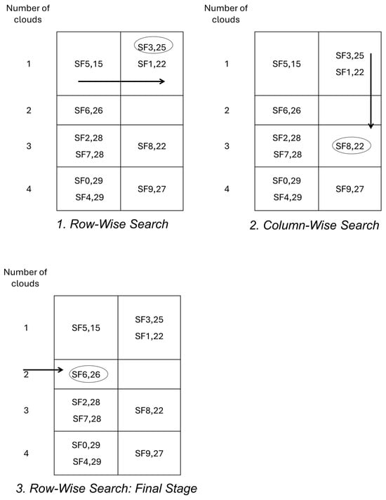
Figure 10. Search process (Each entry, such as SF1,22, represents a SF(SF Number, Composition Frequency).

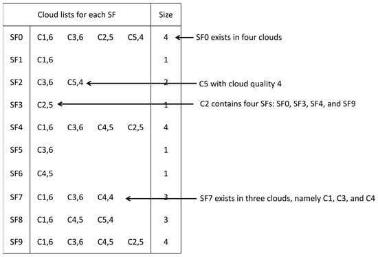
Figure 11. Cloud list (Each entry, such as C1,6, represents a Cloud (Cloud Number, Quality).

4.6. Complexity Analysis

This section elaborates on the computational complexities of the service table creation, the cloud lists, the SF table, and the search process. The complexity analysis helps determine the overall contribution towards the computational cost.

The creation of the service table is a foundational operation executed only once at the start, and the service table categorizes services based on their quality levels, with a time complexity O(n² × log(n)), where n represents the number of services, respectively. This process iterates through all services and subsequently sorts the services by their quality after their addition to the service table. The space complexity is equal to the number of services, which is O(n).

The creation of cloud lists is a crucial foundational step, which is performed once at the outset to facilitate efficient cloud selection based on quality metrics. As the algorithm uses a nested iterative process, it commences with iterations over each cloud. Within each cloud iteration, an inner loop traverses through each SF, resulting in a combined iteration complexity of O(nc × nf), where nc indicates the number of clouds and nf indicates the number of SFs. The cloud list structure retains a collection of SFs, each linked to their respective clouds, resulting in a space complexity equal to O(nf).

The SF table initialization process involves iterating over SFs in the cloud list to determine the required rows for the creation of the SF table and then populating the SF table with SFs. The SF table is enhanced by including the columns and organizing the SFs according to composition frequency. This setup results in a complexity of O(nf² × log(nf)). The space complexity is equal to the number of SFs, which is O(nf).

The search process iteratively scans the SF table to locate the requested SFs and retrieve associated clouds and services from the cloud list and service table. This process operates with a time complexity of O(nf), guaranteeing an efficient composition.

To conclude the complexities, each component contributes unique computational complexities. The overall time complexity is influenced by the creation of the service table, resulting in O(n² × log(n)), while the space complexity is highly influenced by O(n). This holistic approach ensures the computational efficiency and scalability of the proposed method.

5. Experimental Methodology

This section presents a comprehensive evaluation framework to validate the effectiveness of the proposed chemistry-based approach (CA) for multi-cloud service composition. The evaluation examines the algorithm’s performance across multiple dimensions, including resource utilization efficiency, computational overhead, and quality of service optimization. The algorithm’s effectiveness is demonstrated through controlled experiments in minimizing combined clouds while maintaining high QoS standards, its computational efficiency in examining clouds and services, and its scalability across different problem sizes.

5.1. Experimental Setup

Several controlled environment experiments were carried out to evaluate the effectiveness of the CA. The experiments were conducted on an Intel Core i7-10700K processor with 32GB RAM running Ubuntu 20.04 LTS, with the CA algorithm being implemented in Python 3.8. The experimental setup follows a simulation-based approach similar to that in [46]. Synthetic datasets were generated with varying numbers of clouds, SFs, and services, across three scenarios: small, moderate, and large. Table 6 summarizes the three experiment scenarios—small, moderate, and large setups—while detailed descriptions of these experimental settings are presented in Table 7.

Table 6. Experimental scenario for algorithm evaluation.

Experimental Scenario	Number of Clouds	Number of Services	Number of SFs	Service Request Range
Small	10	5000	50	10–80
Moderate	15	10,000	100	10–80
Large	20	20,000	200	10–80

Table 7. Description of experimental settings.

Parameter	Definition
Number of clouds	Number of clouds in a given experimental scenario
Number of services	Number of services, a subset of SFs, performing similar tasks with different QoSs
Number of SFs	Number of SFs describing service tasks
Number of requests	Number of user requests containing a set of SFs (e.g., R1 = {SF1, SF2, SF3})

Table 8 outlines the QoS value ranges used for each service. To evaluate the algorithm’s scalability, experimental scenarios featured increasing numbers of clouds, SFs, and services were used, with the number of user requests ranging from 10 to 80.

Table 8. QoS value ranges.

Factor	Initial Values
Response time	A random number between 20 and 1500 (normal distribution)
Cost	A random number between 2 and 15 (normal distribution)
Availability	A random number between 0.95 and 1 (normal distribution)
Reliability	A random number between 0.4 and 1 (normal distribution)

The experimental datasets were generated using controlled random generation, with QoS parameters following normal distributions within realistic ranges, as detailed in Table 8. To ensure comprehensive testing, each experiment was repeated 30 times, with results reporting means and standard deviations at a 95% confidence level.

5.2. Performance Metrics

For each scenario, five performance metrics were assessed: the total number of clouds utilized in the composite service (NC), the overall number of clouds examined throughout the service composition process (NEC), the total number of services examined to fulfill requests (NES), execution time, and fitness. The fitness metric, which is calculated using Equation (5), evaluates the overall quality of the composite service by computing QoS metrics, as shown in Table 9.

Table 9. Calculating the sequential pattern of QoS attributes.

Response Time	Availability	Cost	Reliability
${\displaystyle \sum _{i=1}^n}{T}_i$	${\displaystyle \prod _{i=1}^n}{A}_i$	${\displaystyle \sum _{i=1}^n}{C}_i$	${\displaystyle \prod _{i=1}^n}{R}_i$

5.3. Data Analysis and Sensitivity Evaluation

To examine the statistical characteristics of the experimental scenarios, we analyzed the following three key aspects:

(1)

the distribution of SFs across clouds;

(2)

the distribution of services across SFs;

(3)

the statistical properties of QoS parameters that influence the optimization objective.

These evaluations help ensure balanced input, avoid bias, and determine sensitivity across QoS factors in the optimization process.

From Table 10, in the small scenario, the SFs are evenly distributed across clouds, with both mean and median values at 6 and a low standard deviation of 1.63. The moderate and large scenarios exhibit higher variability, as indicated by the increased standard deviations. However, all clouds actively participate in service composition, suggesting a well-balanced structure that minimizes bottlenecks and ensures equitable cloud utilization.

Table 10. Statistical summary of SFs per cloud.

Experimental Scenario	Total SFs	Std Dev	Median	Mean	Max	Min
Small	60	1.63	4	9	6	6
Moderate	100	2.98	5	16	10	10
Large	200	6.26	10	32	20	20

From Table 11, the small scenario demonstrates a nearly uniform distribution of services among SFs, with a minimal standard deviation of 0.54 and a narrow range between 83 and 85. The moderate scenario maintains this uniformity with slightly increased variability. Conversely, the large scenario exhibits a broader range (50–300) and a higher standard deviation of 46.21, indicating a more heterogeneous distribution. This variability in the large scenario could introduce complexity in service selection during composition.

Table 11. Statistical summary of services per SF.

Experimental Scenario	Total Services	Std Dev	Median	Mean	Max	Min
Small	5000	0.54	83	83.33	85	83
Moderate	10,000	1.02	67	66.83	71	66
Large	20,000	46.21	100	100	300	50

Table 12 summarizes the statistical measures of key QoS parameters—response time, availability, cost, and reliability—across the experimental scenarios.

Table 12. Statistical comparison of QoSs in experimental scenarios.

Experimental Scenario	Statistical Measure	Response Time	Availability	Cost	Reliability
Small	mean	830.52	0.97	8.69	0.69
	std	460.98	0.02	4.08	0.19
	min	21	0.95	2	0.4
	max	1500	1	15	1
Moderate	mean	819.85	0.97	8.61	0.67
	std	459.56	0.02	4.11	0.19
	min	20	0.95	2	0.4
	max	1500	1	15	1
Large	mean	840.75	0.97	8.72	0.67
	std	461.65	0.02	4.12	0.19
	min	20	0.95	2	0.4
	max	1500	1	15	1

The analysis of QoS parameters reveals the following insights.

Response Time: This exhibits significant variability across all scenarios, with a wide range (20–1500 ms) and high standard deviations (~460 ms). This indicates the need for normalization during fitness computation to manage the impact of extreme values.

Availability: This demonstrates high stability, with values tightly clustered between 0.95 and 1.00, with a low standard deviation of 0.02. This consistency suggests that availability is a reliable parameter across different scenarios.

Cost: This shows considerable spread, ranging from 2.00 to 15.00, with standard deviations exceeding 4.00. This indicates that cost is a discriminative factor in service selection and may introduce sensitivity in optimization.

Reliability: This caries moderately, ranging from 0.40 to 1.00, with a standard deviation of 0.19. This suggests differentiated service behavior under stress, making reliability a sensitive discriminator in the selection process.

The system is most sensitive to variations in response time, cost, and reliability, as observed through the wide data spread and higher standard deviations across all scenarios. These fluctuations demand normalization to ensure balanced fitness computation and to avoid the dominance of any single QoS metric. In contrast, availability remains remarkably stable, exhibiting minimal variation, thus contributing a low sensitivity. The CA normalized and equally weighted QoSs during quality assessment. This ensures that highly sensitive parameters such as response time or cost do not overshadow others, maintaining fairness and preventing bias.

The distribution of SFs across clouds in Table 10 is nearly uniform, especially in the small and moderate scenarios, leading to low sensitivity. However, as shown in Table 11, the distribution of services per SF becomes increasingly variable in the large scenario, introducing moderate sensitivity that can complicate service selection. The CA structures allow us to avoid such sensitivity by utilizing different structures to select SFs, clouds, and services based on their cloud number, composition frequencies, cloud quality, and QoS levels. Table 13 provides a summary of the distribution patterns and sensitivity levels across different aspects of the cloud service composition.

Table 13. Summary of distribution patterns and sensitivity levels.

Aspect	Distribution Pattern	Sensitivity Level
SFs per cloud	Nearly uniform	Low
Services per SF	Highly uniform (small), varied (large)	Very low to medium
Response time	Wide spread	High
Availability	Narrow spread	Low
Cost	Wide spread	High
Reliability	Moderate spread	Medium

5.4. Initial Configuration of the Considered Algorithms

The comparative algorithms used are the Genetic Algorithm (GA), Simulated Annealing (SA), and Tabu Search (TS). These were selected because they are widely used and well-established metaheuristic optimization methods for service composition problems, and without them, the comparison will be useless. Another reason for selecting these algorithms is their inclusion and application in [57]. The authors applied them to a similar context of multi-objective service compositions with QoS considerations. It was ensured that a diverse range of benchmark methods were added that were representative of current state-of-the-art techniques.

Furthermore, each algorithm represents a different heuristic family, i.e., evolutionary (GA), physics-inspired (SA), and memory-based (TS), allowing for a comprehensive performance evaluation of our proposed CA across diverse optimization paradigms.

To provide a comprehensive comparative analysis, the CA is evaluated against three state-of-the-art service composition algorithms: GA, SA, and TS. The GA implementation used a population size of 100 with a crossover probability of 0.8 and a mutation probability ranging from 0.2 to 0.9. The SA algorithm was configured with an initial temperature of 100,000 and a cooling schedule ranging from 0.15 to 0.9, while the TS implementation employed a tabu tenure of 20–100 steps. The CA and CA2 algorithms were configured with a fixed number of columns in the SF table, which were set to 1 and 2, respectively. The CA algorithm represents the initial configuration, utilizing a single column, while the CA2 algorithm reflects the state after processing the maximum number of requests, with two columns. Table 14 presents the complete configuration details for all the algorithms considered in this study.

Table 14. Initial configuration of each algorithm.

No.	Algorithm	Parameter
1.	CA	Configured with a fixed number of columns in the SF table, set to 1.
2.	CA2	Configured with a fixed number of columns in the SF table, set to 2.
3.	GA	Population size: 100; Crossover probability: 0.8; Mutation probability: 0.2 to 0.9 (step size of 0.1); A total of 250 iterations per request.
4.	SA	Initial temperature: 100,000; Cooling schedule: ranges from 0.15 to 0.9 (step size of 0.15); Initial solution generated by executing TS 10 times to avoid falling in local optima.
5.	TS	Tabu tenure: 20 to 100 (step size of 10); A total of 250 iterations per request.
6.	Elitism	Used in all algorithms except CA and CA2 to prevent the loss of the best-found solution.

Each algorithm was executed for 250 iterations per request to ensure fair comparison. To prevent the loss of the best-found solution, elitism was implemented in all algorithms except CA and CA2. The experimental results and their analysis are presented in Section 6, which demonstrates the effectiveness of the proposed work across different operational scenarios and performance metrics.

6. Results and Discussion

The following section outlines the findings of the CA for service composition in an MCE, as detailed in Section 6.1. Section 6.2 provides a comprehensive analysis of these results, evaluating key findings to validate the algorithm’s effectiveness across diverse scenarios. The analysis highlights the algorithm’s efficiency and offers insights into its scalability, reliability, and applicability to various service composition problems, particularly in complex and large-scale environments.

6.1. Experimental Results

To evaluate service composition in a controlled setting, a series of experiments in an MCE were performed, utilizing the CA and additional benchmark algorithms in three different experimental scenarios (shown in Table 6). The algorithm’s performance is evaluated in terms of execution time, fitness, NC, NEC, and NES. Three well-known service composition algorithms—SA, GA, and TS—were employed as benchmarks in this research.

The following subsections describe the performance metrics for each scenario.

6.1.1. Number of Combined Clouds

Figure 12 shows the algorithms’ performance evaluation of NC. The algorithms showed a consistent increase in NC as the number of requests rose. The CA and CA2 algorithms achieved the lowest NC values across all experimental scenarios, with CA slightly outperforming CA2, as the number of requests increased from 30 to 80. In contrast, GA, TS, and SA displayed similar results but examined more combined clouds than CA and CA2. Among these, the TS algorithm exhibited a slightly lower NC value in all scenarios when compared to GA and SA.

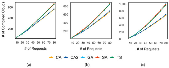
Figure 12. Number of combined clouds vs. number of requests: (a) Scenario 1—Small: 10 clouds, 5000 services, 50 SFs, requests 10–80, (b) scenario 2—Moderate: 15 clouds, 10,000 services, 100 SFs, requests 10–80, and (c) scenario 3—Large: 20 clouds, 20,000 services, 200 SFs, requests 10–80.

As the total number of requests reached 80, the NC gap between CA/CA2 and the other algorithms became noticeable, increasing by approximately 100 in scenario 1, 200 in scenario 2, and 300 in scenario 3.

6.1.2. Number of Examined Clouds

Figure 13 illustrates the NEC performance of the proposed CA and benchmark algorithms across various scenarios. As the number of requests increased, these algorithms showed significant increases in NEC. CA and CA2 consistently achieved the lowest NEC values, indicating superior computational efficiency. TS displayed poor performance, reflecting higher computational costs, while GA performed moderately compared to the other algorithms. Notably, SA examined more clouds than GA, yet maintained a good performance.

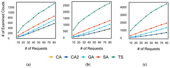
Figure 13. Number of examined clouds vs. number of requests: (a) Scenario 1—Small: 10 clouds, 5000 services, 50 SFs, requests 10–80, (b) scenario 2—Moderate: 15 clouds, 10,000 services, 100 SFs, requests 10–80, and (c) scenario 3—Large: 20 clouds, 20,000 services, 200 SFs, requests 10–80.

It is also worth noting that the NEC gap between CA/CA2 and TS widened significantly across various scenarios, reaching approximately 800, 2000, and 4000 for scenarios 1, 2, and 3, respectively, when processing 80 requests. This demonstrated the computational efficiency of the CA compared to the other algorithms.

6.1.3. Number of Examined Services

The NES performance evaluation of the suggested and benchmark algorithms is presented in Figure 14. While all algorithms showed an increase in NES as the number of requests grew, CA and CA2 maintained the slowest rate of increase. Both algorithms consistently examined the fewest NES, even at higher request levels. Although not as effective as CA/CA2, SA also performed well. TS exhibited moderate performance, examining fewer services than GA but more than SA and the CA algorithms. The GA consistently examined the highest NES, with an exponential increase as the number of requests rose.

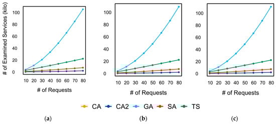
Figure 14. Number of examined services vs. number of requests: (a) Scenario 1—Small: 10 clouds, 5000 services, 50 SFs, requests 10–80, (b) scenario 2—Moderate: 15 clouds, 10,000 services, 100 SFs, requests 10–80, and (c) scenario 3—Large: 20 clouds, 20,000 services, 200 SFs, requests 10–80.

6.1.4. Execution Time

Figure 15 compares the execution times of the algorithms. Execution time increased for all algorithms as the number of requests rose. In both scenarios 1 and 2, CA had the shortest execution time, followed by CA2. The TS execution time increased by nearly 6 ms as the total number of requests increased. TS and SA displayed similar execution times, while the GA consistently had the longest execution time.

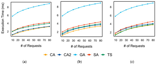
Figure 15. Execution time vs. number of requests: (a) Scenario 1—Small: 10 clouds, 5000 services, 50 SFs, requests 10–80, (b) scenario 2—Moderate: 15 clouds, 10,000 services, 100 SFs, requests 10–80, and (c) scenario 3—Large: 20 clouds, 20,000 services, 200 SFs, requests 10–80.

The execution times of all algorithms in scenario 3 are shown in Figure 15c, with TS and CA having the shortest execution times, followed by CA2 and SA. The GA exhibited a consistent performance with the highest execution time.

The execution times do not account for the time required to generate the support utilized in CA/CA2 (e.g., SF table, service table, frequency matrix, and cloud list). Even when including this preparation time in the overall execution time with 80 requests, CA and CA2 maintained the same performance pattern. In scenarios 1 and 2, CA had the fastest execution time, followed by CA2. Similarly, CA and TS achieved the shortest execution time in scenario 3. CA2 continued to rank third in terms of performance, following TS and CA. Table 15 details the amount of time required to generate the structures for CA and CA2.

Table 15. CA and CA2 structure generation times.

Dataset/Time (ms)	Structure of CA	Structure of CA2
1	0.16	0.53
2	0.2	0.85
3	0.6	1.39

6.1.5. Fitness

Figure 16a depicts the performance evaluation of the proposed and benchmark algorithms in scenario 1 based on fitness metrics. For a low number of requests, the CA and CA2 algorithms demonstrated high fitness values. However, as the number of requests increased, their fitness values decreased. After processing 70 requests, the fitness levels of CA and CA2 fell below those of TS. At this point, TS performance was on par with that of the CA and CA2 algorithms. Beyond this point, the TS fitness values increased. SA initially showed greater fitness, but its performance declined once the number of requests reached 60 or more. The GA, which initially had lower fitness values, eventually outperformed SA after 60 requests.

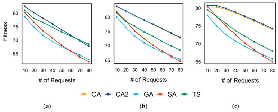
Figure 16. Fitness vs. number of requests: (a) Scenario 1—Small: 10 clouds, 5000 services, 50 SFs, requests 10–80, (b) scenario 2—Moderate: 15 clouds, 10,000 services, 100 SFs, requests 10–80, and (c) scenario 3—Large: 20 clouds, 20,000 services, 200 SFs, requests 10–80.

Figure 16b,c present the fitness performance of the proposed and benchmark algorithms in scenarios 2 and 3. The fitness values of CA and CA2 consistently exceeded those of the other algorithms. While SA originally exhibited greater fitness than TS, its performance diminished after 30 requests and continued to decline beyond 70 requests, eventually falling below the GA. In scenarios with a smaller number of requests, TS initially exhibited lower fitness levels compared to SA. However, SA surpassed TS after processing 30 or more requests. Ultimately, the GA outperformed SA after processing 70 requests, despite having lower fitness values in the initial stages.

Table 16 summarizes the results of the CA compared to the benchmark algorithms (SA, GA, and TS) across the key performance metrics. The metrics used are NC, NEC, NES, execution time, and fitness. Improvement in terms of percentage is used for the efficiency calculations of CA over other algorithms. The key results achieved are enumerated below.

Table 16. Comparison table of CA enhancement over benchmark algorithms.

Metric	Algorithm	Scenario 1 (Small)	Scenario 2 (Moderate)	Scenario 3 (Large)
Number of Combined Clouds (NEC)	GA	15%	22%	33%
	SA	15%	23%	33%
	TS	14%	22%	31%
Number of Examined Clouds (NEC)	GA	20%	35%	50%
	SA	34%	50%	65%
	TS	58%	75%	85%
Number of Examined Services (NES)	GA	98%	98%	98%
	SA	74%	74%	74%
	TS	92%	92%	92%
Execution Time (ms)	GA	99%	99%	99%
	SA	67%	63%	54%
	TS	56%	43%	10%
Fitness	GA	8%	11%	12%
	SA	9%	12%	14%
	TS	1%	6%	9%

• CA dominantly outperforms all benchmark algorithms in terms of NC, NEC, NES, execution time, and fitness across all scenarios.
• The efficiency improvement in the CA is greater in relation to NES, execution time, and NEC. It has shown a 10–99% better performance when compared to the GA, SA, and TS.
• Fitness values for CA are also higher, which indicates a better solution quality. Numerically speaking, an improvement of 1–14% over other algorithms is observed.
• It was revealed that TS performs well in terms of fitness. However, it was also observed that TS is more resource-hungry, making it less efficient than CA.
• The GA has the worst performance in terms of execution time and NES. This can be an unsuitable approach for large-scale real-world environments.

6.2. Discussions

The results of the comprehensive experiment revealed key insights into the performance of the CA compared to benchmarks across metrics such as NC, NEC, NES, fitness, and execution times in three different scenarios. The findings indicate that the CA and benchmarks performed differently in various scenarios with varying workload requests. Based on the results, the CA consistently maintained QoS solutions while outperforming benchmark methods, particularly in terms of lower computational costs across various scenarios and request counts. Despite the increasing complexity of the service composition problem, the CA achieved rapid execution times; low NC, NEC, and NES values; and high fitness across a range of experimental scenarios. In light of these findings, CA is the recommended algorithm for achieving high-quality results in resource-constrained environments.

As the number of requests increased, the performance advantage of the CA over other algorithms became increasingly evident, highlighting its scalability and flexibility in addressing complex service composition challenges. The algorithm exhibited a linear increase in execution time while consistently maintaining lower values for NC, NEC, and NES, alongside high solution quality. This demonstrates the CA’s practicality and reliability for large-scale and real-time applications.

The proposed chemistry-based algorithm (CA) is designed to be scalable, from the beginning. This was also demonstrated in Section 6 by testing the proposed approach against three scenarios (small, moderate, and large). These scenarios scale from 5000 to 20,000 services and from 10 to 20 clouds. It was ensured that low execution times and high fitness values were maintained. The scalability is achieved through the algorithm’s structured decomposition of the search space, and the use of pre-generated SF tables and QoS-ranked service lists significantly reduces computational overhead. Moreover, as the number of requests increased, CA consistently maintained lower NEC, NES, and NC values compared to benchmark algorithms (GA, SA, and TS), confirming its efficiency in large-scale environments and making it a strong contender for usage. These results confirm that the CA scales well with problem size while preserving performance and solution quality.

In contrast, the GA’s ability to explore the solution space resulted in high NES and execution times. Although the GA exhibited a moderate NEC and high NES, it still had trouble achieving optimal fitness values, particularly when the volume of requests increased. A key factor in the GA’s reduced performance is premature convergence. The GA starts with a randomly generated population, which may be lacking in diversity or high-quality initial solutions. This limitation can make it more difficult for the algorithm to effectively explore the solution space, which can lead to premature convergence to suboptimal solutions. Although the purpose of mutation and crossover processes is to ensure variety and improve solutions, their performance is impacted by the quality and variety of the initial population. As a result, the GA’s extensive exploration led to longer execution times, making it less suitable for real-time or large-scale applications.

In the experiments, it was revealed that the TS algorithm offers a well-rounded approach, striking an ideal balance between efficiency and exploration. Its NES values were moderate—generally higher than CA/CA2 but lower than the GA—while its execution time was better than the GA and comparable to CA/CA2. TS avoided local optima and achieved competitive fitness across a variety of experimental scenarios. However, its linear growth in both execution time and NES implies that while it scales well, it still requires more computational resources than CA and CA2. Furthermore, TS yielded the largest NEC values. Notably, after processing 70 requests, TS sometimes performed better than CA2, demonstrating its ability to preserve solution quality in high-request scenarios. This suggests that TS is a viable option when computational resources are adequate.

The SA algorithm provided a middle ground, outperforming the GA in efficiency and achieving comparable fitness values due to its moderate NEC, NES, and execution time. Nevertheless, it did not outperform CA/CA2 in all situations.

In summary, the experimental results confirm that CA and CA2 are the most reliable and scalable algorithms, particularly in complex, large-scale environments where both computational efficiency and solution quality are critical. In most scenarios, CA and CA2 achieved the highest fitness values, as well as the lowest values for NC, NES, NEC, and execution time. TS, on the other hand, proved to be a suitable choice for situations where high-quality solutions were a priority and computational resources were abundant, as it delivered competitive fitness values at the expense of increased computational effort. The GA, despite its extensive exploration, underperformed in terms of fitness and had long execution times, making it unsuitable for large-scale cloud service composition. The performance of SA was mediocre, combining efficiency and fitness, but it lagged behind both CA/CA2 and TS.

7. Conclusions and Future Work

This research presents a novel chemistry-based approach (CA) that addresses the complexities of multi-cloud environment-based service composition. Taking inspiration from the periodic table and electron motion principles, the proposed method systematically organizes and optimizes service selection. This enables a significant reduction in the search space while preserving the solution quality. In our experiments, it was deduced that the CA demonstrates superior efficiency compared to state-of-the-art algorithms, as well as evaluating fewer cloud resources and services while achieving better execution times and fitness levels. The superior performance across different scenarios attests to the method’s effectiveness not only in resource management and service composition but also in establishing a solid foundation for practical implementation in cloud computing systems.

In any technological research, there may be some limitations. In the proposed work, we have identified some limitations that need attention. First of all, to construct and maintain SFs and service tables, there is a significant amount of preprocessing involved. This pre-processing adds additional computational overhead during the start of the deployment, especially in large-scale systems. Another limitation observed is that the current implementation shows reduced effectiveness where Service Files are uniformly distributed across clouds or attain identical quality metrics, which makes the structured tables redundant. These limitations are natural considering the algorithm’s dependence on static organizational principles. Furthermore, this dependence may not allow for the adaptation to environments with highly dynamic service characteristics or highly balanced resource distributions.

In the future, we intend to enhance the algorithm’s adaptability and scalability. For those reasons, a key improvement requirement is to develop dynamic data structures. These data structures should automatically adjust table configurations based on real-time service availability and quality changes in order to eliminate the current dependency on static arrangements. Furthermore, we will also explore the possibility of using a distributed broker system instead of a single-broker model. Moreover, integration with machine learning techniques will be studied for the possibility to enable intelligent and context-aware service composition in dynamic environments. The satisfactory results achieved in cloud environments also suggest potential applications in other computing environments such as fog computing architectures, where challenges such as resource optimization exist.

References

- Wu, Z. Service Computing: Concept, Method and Technology; Academic Press: Cambridge, MA, USA, 2014. [Google Scholar]
- Wiesner, K.; Vaculín, R.; Kollingbaum, M.; Sycara, K. Recovery mechanisms for semantic web services. In Lecture Notes in Computer Science, Proceedings of the IFIP International Conference on Distributed Applications and Interoperable Systems, Oslo, Norway, 4–6 June 2008; Goos, G., Ed.; Springer: Berlin/Heidelberg, Germany, 2008; pp. 100–105. [Google Scholar]
- Sheng, J.; Hu, Y.; Zhou, W.; Zhu, L.; Jin, B.; Wang, J.; Wang, X. Learning to schedule multi-NUMA virtual machines via reinforcement learning. Pattern Recognit. 2022, 121, 108254. [Google Scholar] [CrossRef]
- Yu, X.; Zhu, M.; Zhu, M.; Zhou, X.; Long, L. Location-aware job scheduling for IoT systems using cloud and fog. Alex. Eng. J. 2025, 110, 346–362. [Google Scholar] [CrossRef]
- Heidari, M.; Emadi, S. Services composition in multi-cloud environments using the skyline service algorithm. Int. J. Eng. 2021, 34, 56–65. [Google Scholar]
- Ramalingam, C.; Mohan, P. Addressing semantics standards for cloud portability and interoperability in multi cloud environment. Symmetry 2021, 13, 317. [Google Scholar] [CrossRef]
- Feng, B.; Ding, Z. Application-oriented cloud workload prediction: A survey and new perspectives. Tsinghua Sci. Technol. 2024, 30, 34–54. [Google Scholar] [CrossRef]
- Hayyolalam, V.; Kazem, A.A.P. A systematic literature review on QoS-aware service composition and selection in cloud environment. J. Netw. Comput. Appl. 2018, 110, 52–74. [Google Scholar] [CrossRef]
- Jatoth, C.; Gangadharan, G.R.; Buyya, R. Computational intelligence based QoS-aware web service composition: A systematic literature review. IEEE Trans. Serv. Comput. 2015, 10, 475–492. [Google Scholar] [CrossRef]
- Thakur, K.; Kumar, G. Nature inspired techniques and applications in intrusion detection systems: Recent progress and updated perspective. Arch. Comput. Methods Eng. 2021, 28, 2897–2919. [Google Scholar] [CrossRef]
- Saji, Y.; Riffi, M.E. A comparative study of three nature-inspired algorithms using the Euclidean travelling salesman problem. In Lecture Notes in Electrical Engineering, Proceedings of the Mediterranean Conference on Information & Communication Technologies 2015, Saïdia, Morocco, 7–9 May 2015; El Oualkadi, A., Choubani, F., El Moussati, A., Eds.; Springer: Berlin/Heidelberg, Germany, 2016; pp. 327–335. [Google Scholar]
- Bejinariu, S.-I.; Rotaru, F.; Luca, R.; Niţă, C.D.; Costin, H. Black hole vs particle swarm optimization. In Proceedings of the 10th International Conference on Electronics, Computers and Artificial Intelligence (ECAI), Iasi, Romania, 28–30 June 2018; pp. 1–6. [Google Scholar]
- Yu, Q.; Chen, L.; Li, B. Ant colony optimization applied to web service compositions in cloud computing. Comput. Electr. Eng. 2015, 41, 18–27. [Google Scholar] [CrossRef]
- Kurdi, H.; Ezzat, F.; Altoaimy, L.; Ahmed, S.H.; Youcef-Toumi, K. MultiCuckoo: Multi-cloud service composition using a cuckoo-inspired algorithm for the Internet of Things applications. IEEE Access 2018, 6, 56737–56749. [Google Scholar] [CrossRef]
- Kurdi, H.; Al-Anazi, A.; Campbell, C.; Al Faries, A. A combinatorial optimization algorithm for multiple cloud service composition. Comput. Electr. Eng. 2015, 42, 107–113. [Google Scholar] [CrossRef]
- Yin, H.; Hao, Y. An energy-aware multi-target service composition method in a multi-cloud environment. IEEE Access 2020, 8, 196567–196577. [Google Scholar] [CrossRef]
- Souri, A.; Rahmani, A.M.; Navimipour, N.J.; Rezaei, R. A hybrid formal verification approach for QoS-aware multi-cloud service composition. Clust. Comput. 2020, 23, 2453–2470. [Google Scholar] [CrossRef]
- Cassar, G.; Barnaghi, P.; Wang, W.; De, S.; Moessner, K. Composition of services in pervasive environments: A divide and conquer approach. In Proceedings of the IEEE Symposium on Computers and Communications (ISCC), Split, Croatia, 7–10 July 2013; pp. 000226–000232. [Google Scholar]
- Shang, J.; Liu, L.; Wu, C. WSCN: Web service composition based on complex networks. In Proceedings of the 2013 International Conference on Service Sciences (ICSS), Shenzhen, China, 11–13 April 2013; pp. 208–213. [Google Scholar]
- Ghobaei-Arani, M.; Souri, A. LP-WSC: A linear programming approach for web service composition in geographically distributed cloud environments. J. Supercomput. 2019, 75, 2603–2628. [Google Scholar] [CrossRef]
- Guidara, I.; Guermouche, N.; Chaari, T.; Jmaiel, M. Time-aware selection approach for service composition based on pruning and improvement techniques. Softw. Qual. J. 2020, 28, 1245–1277. [Google Scholar] [CrossRef]
- Mezni, H.; Sellami, M. Multi-cloud service composition using formal concept analysis. J. Syst. Softw. 2017, 134, 138–152. [Google Scholar] [CrossRef]
- Nazari, Z.; Kamandi, A.; Shabankhah, M. An optimal service composition algorithm in multi-cloud environment. In Proceedings of the 5th International Conference on Web Research (ICWR), Tehran, Iran, 24–25 April 2019; pp. 141–151. [Google Scholar]
- Rajakumar, R.; Dhavachelvan, P.; Vengattaraman, T. A survey on nature inspired meta-heuristic algorithms with its domain specifications. In Proceedings of the International Conference on Communication and Electronics Systems (ICCES), Coimbatore, India, 21–22 October 2016; pp. 1–6. [Google Scholar]
- Wang, L.; Shen, J. A systematic review of bio-inspired service concretization. IEEE Trans. Serv. Comput. 2015, 10, 493–505. [Google Scholar] [CrossRef]
- Tang, M.; Ai, L. A hybrid genetic algorithm for the optimal constrained web service selection problem in web service composition. In Proceedings of the IEEE Congress on Evolutionary Computation, Barcelona, Spain, 18–23 July 2010; pp. 1–8. [Google Scholar]
- Grati, R.; Boukadi, K.; Ben-Abdallah, H. QoS based resource allocation and service selection in the cloud. In Proceedings of the 11th International Conference on e-Business (ICE-B), Vienna, Austria, 28–30 August 2014; pp. 249–256. [Google Scholar]
- Wang, D.; Yang, Y.; Mi, Z. A genetic-based approach to web service composition in geo-distributed cloud environment. Comput. Electr. Eng. 2015, 43, 129–141. [Google Scholar] [CrossRef]
- Jatoth, C.; Gangadharan, G.R.; Buyya, R. Optimal fitness aware cloud service composition using an adaptive genotypes evolution based genetic algorithm. Future Gener. Comput. Syst. 2019, 94, 185–198. [Google Scholar] [CrossRef]
- Sadeghiram, S.; Ma, H.; Chen, G. Multi-objective distributed Web service composition—A link-dominance driven evolutionary approach. Future Gener. Comput. Syst. 2023, 143, 163–178. [Google Scholar] [CrossRef]
- Wang, H.; Du, Y.; Chen, F. A hybrid strategy improved SPEA2 algorithm for multi-objective web service composition. Appl. Sci. 2024, 14, 4157. [Google Scholar] [CrossRef]
- Wang, H.; Du, Y. An Adaptive Mutation Strategy Improved SPEA2 Algorithm for Multi-objective Web Service Composition. In Proceedings of the 2024 3rd International Symposium on Robotics, Artificial Intelligence and Information Engineering, Singapore, 5–7 July 2024; pp. 15–20. [Google Scholar]
- Garcia, N.P.; Duran, F.; Berrocal, K.M.; Pimentel, E. Location-aware scalable service composition. Softw.-Pract. Exp. 2023, 53, 2408–2429. [Google Scholar] [CrossRef]
- Sadeghiram, S.; Ma, H.; Chen, G. Cluster-guided genetic algorithm for distributed data-intensive web service composition. In Proceedings of the IEEE Congress on Evolutionary Computation (CEC), Rio de Janeiro, Brazil, 8–13 July 2018; pp. 1–7. [Google Scholar]
- Zhang, W.; Guo, H.; Zeng, Z.; Qi, Y.; Wang, Y. Transportation cloud service composition based on fuzzy programming and genetic algorithm. Transp. Res. Rec. 2018, 2672, 64–75. [Google Scholar] [CrossRef]
- Amiri, M.A.; Serajzadeh, H. Effective web service composition using particle swarm optimization algorithm. In Proceedings of the 6th International Symposium on Telecommunications (IST), Tehran, Iran, 6–8 November 2012; pp. 1190–1194. [Google Scholar]
- Gao, H.; Zhang, K.; Yang, J.; Wu, F.; Liu, H. Applying improved particle swarm optimization for dynamic service composition focusing on quality of service evaluations under hybrid networks. Int. J. Distrib. Sens. Netw. 2018, 14, 1550147718761583. [Google Scholar] [CrossRef]
- Balakrishnan, S.M.; Sangaiah, A.K. Integrated QoUE and QoS approach for optimal service composition selection in internet of services (IoS). Multimed. Tools Appl. 2017, 76, 22889–22916. [Google Scholar] [CrossRef]
- Dahan, F. An effective multi-agent ant colony optimization algorithm for QoS-aware cloud service composition. IEEE Access 2021, 9, 17196–17207. [Google Scholar] [CrossRef]
- Alayed, H.; Dahan, F.; Alfakih, T.; Mathkour, H.; Arafah, M. Enhancement of ant colony optimization for QoS-aware web service selection. IEEE Access 2019, 7, 97041–97051. [Google Scholar] [CrossRef]
- Wang, X.; Xu, X.; Sheng, Q.Z.; Wang, Z.; Yao, L. Novel artificial bee colony algorithms for QoS-aware service selection. IEEE Trans. Serv. Comput. 2016, 12, 247–261. [Google Scholar] [CrossRef]
- Huo, L.; Wang, Z. Service composition instantiation based on cross-modified artificial bee colony algorithm. China Commun. 2016, 13, 233–244. [Google Scholar] [CrossRef]
- Zhang, Y.; Cui, G.; Wang, Y.; Guo, X.; Zhao, S. An optimization algorithm for service composition based on an improved FOA. Tinshhua Sci. Technol. 2015, 20, 90–99. [Google Scholar] [CrossRef]
- Seghir, F.; Khababa, A. A hybrid approach using genetic and fruit fly optimization algorithms for QoS-aware cloud service composition. J. Intell. Manuf. 2018, 29, 1773–1792. [Google Scholar] [CrossRef]
- Li, J.; Yu, B.; Chen, W. Research on intelligence optimization of web service composition for QoS. In Communications in Computer and Information Science, Proceedings of the International Conference on Information Computing and Applications, Chengde, China, 14–16 September 2012; Li, G., Filipe, J., Xu, Z., Eds.; Springer: Berlin/Heidelberg, Germany, 2012; pp. 227–235. [Google Scholar]
- Ghobaei-Arani, M.; Rahmanian, A.A.; Aslanpour, M.S.; Dashti, S.E. CSA-WSC: Cuckoo search algorithm for web service composition in cloud environments. Soft Comput. 2018, 22, 8353–8378. [Google Scholar] [CrossRef]
- Wang, H.; Yang, D.; Yu, Q.; Tao, Y. Integrating modified cuckoo algorithm and creditability evaluation for QoS-aware service composition. Knowl. Based Syst. 2018, 140, 64–81. [Google Scholar] [CrossRef]
- Bhushan, S.B.; Reddy, P.C.H. A hybrid meta-heuristic approach for QoS-aware cloud service composition. Int. J. Web Serv. Res. IJWSR 2018, 15, 1–20. [Google Scholar] [CrossRef]
- Xia, H.; Chen, Y.; Li, Z.; Gao, H.; Chen, Y. Web service selection algorithm based on particle swarm optimization. In Proceedings of the Eighth IEEE International Conference on Dependable, Autonomic and Secure Computing, Chengdu, China, 12–14 December 2009; pp. 467–472. [Google Scholar]
- Clerc, M.; Kennedy, J. The particle swarm-explosion, stability, and convergence in a multidimensional complex space. IEEE Trans. Evol. Comput. 2002, 6, 58–73. [Google Scholar] [CrossRef]
- Nazif, H.; Nassr, M.; Al-Khafaji, H.M.R.; Navimipour, N.J.; Unal, M. A cloud service composition method using a fuzzy-based particle swarm optimization algorithm. Multimed. Tools Appl. 2024, 83, 56275–56302. [Google Scholar] [CrossRef]
- Tabalvandani, M.A.N.; Shirvani, M.H.; Motameni, H. Reliability-aware web service composition with cost minimization perspective: A multi-objective particle swarm optimization model in multi-cloud scenarios. Soft Comput. 2024, 28, 5173–5196. [Google Scholar] [CrossRef]
- Yuan, S.; Shen, J.; Krishna, A. Ant inspired scalable peer selection in ontology-based service composition. In Proceedings of the World Conference on Services-II, Bangalore, India, 21–25 September 2009; pp. 95–102. [Google Scholar]
- Dahan, F.; El Hindi, K.; Ghoneim, A. An adapted ant-inspired algorithm for enhancing web service composition. Int. J. Semantic Web Inf. Syst. IJSWIS 2017, 13, 181–197. [Google Scholar] [CrossRef]
- Jiang, P.; Liu, F.; Wang, J.; Song, Y. Cuckoo search-designated fractal interpolation functions with winner combination for estimating missing values in time series. Appl. Math. Model. 2016, 40, 9692–9718. [Google Scholar] [CrossRef]
- Fan, X.-Q.; Fang, X.-W.; Jiang, C.-J. Research on web service selection based on cooperative evolution. Expert Syst. Appl. 2011, 38, 9736–9743. [Google Scholar] [CrossRef]
- Liu, S.; Wei, Y.; Tang, K.; Qin, A.K.; Yao, X. QoS-aware long-term based service composition in cloud computing. In Proceedings of the IEEE Congress on Evolutionary Computation (CEC), Sendai, Japan, 25–28 May 2015; pp. 3362–3369. [Google Scholar]
- Deng, S.; Huang, L.; Li, Y.; Zhou, H.; Wu, Z.; Cao, X.; Kataev, M.Y.; Li, L. Toward risk reduction for mobile service composition. IEEE Trans. Cybern. 2016, 46, 1807–1816. [Google Scholar] [CrossRef] [PubMed]
- Niewiadomski, A.; Skaruz, J.; Switalski, P.; Penczek, W. Concrete planning in PlanICS framework by combining SMT with GEO and simulated annealing. Fundam. Informaticae 2016, 147, 289–313. [Google Scholar] [CrossRef]
- Banâtre, J.-P.; Priol, T.; Radenac, Y. Service orchestration using the chemical metaphor. In Lecture Notes in Computer Science, Proceedings of the IFIP International Workshop on Software Technolgies for Embedded and Ubiquitous Systems, Capri Island, Italy, 1–3 October 2008; Goos, G., Ed.; Springer: Berlin/Heidelberg, Germany, 2008; pp. 79–89. [Google Scholar]
- Banâtre, J.-P.; Priol, T.; Radenac, Y. Chemical programming of future service-oriented architectures. J. Softw. 2009, 4, 738–746. [Google Scholar] [CrossRef][Green Version]
- Di Napoli, C.; Giordano, M.; Németh, Z.; Tonellotto, N. Using chemical reactions to model service composition. In Proceedings of the Second International Workshop on Self-Organizing Architectures, Washington, DC, USA, 7 June 2010; pp. 43–50. [Google Scholar]
- Viroli, M.; Casadei, M. Chemical-inspired self-composition of competing services. In Proceedings of the 2010 ACM Symposium on Applied Computing, Sierre, Switzerland, 22–26 March 2010; pp. 2029–2036. [Google Scholar]
- Fernández, H.; Tedeschi, C.; Priol, T. A chemistry-inspired workflow management system for decentralizing workflow execution. IEEE Trans. Serv. Comput. 2013, 9, 213–226. [Google Scholar] [CrossRef]
- Wang, C.; Pazat, J.-L. A chemistry-inspired middleware for self-adaptive service orchestration and choreography. In Proceedings of the 2013 13th IEEE/ACM International Symposium on Cluster, Cloud, and Grid Computing, Delft, The Netherlands, 13–16 May 2013; pp. 426–433. [Google Scholar]
- De Angelis, F.L.; Fernandez-Marquez, J.L.; Di Marzo Serugendo, G. Self-composition of services in pervasive systems: A chemical-inspired approach. In Agent and Multi-Agent Systems: Technologies and Applications, Proceedings of the 8th International Conference KES-AMSTA 2014 Chania, Greece, June 2014; Jezic, G., Kusek, M., Lovrek, I., Howlett, R.J., Jain, L.C., Eds.; Springer: Berlin/Heidelberg, Germany, 2014; pp. 37–46. [Google Scholar]
- Ko, J.M.; Kim, C.O.; Kwon, I.-H. Quality-of-service oriented web service composition algorithm and planning architecture. J. Syst. Softw. 2008, 81, 2079–2090. [Google Scholar] [CrossRef]
- Spezzano, G. Using service clustering and self-adaptive MOPSO-CD for QoS-aware cloud service selection. Procedia Comput. Sci. 2016, 83, 512–519. [Google Scholar] [CrossRef]
- Khanam, R.; Kumar, R.R.; Kumari, B. A novel approach for cloud service composition ensuring global QoS constraints optimization. In Proceedings of the International Conference on Advances in Computing, Communications and Informatics (ICACCI), Bangalore, India, 19–22 September 2018; pp. 1695–1701. [Google Scholar]
- Sefati, S.S.; Halunga, S. A hybrid service selection and composition for cloud computing using the adaptive penalty function in genetic and artificial bee colony algorithm. Sensors 2022, 22, 4873. [Google Scholar] [CrossRef]
- Dahan, F.; Alwabel, A. Artificial bee colony with cuckoo search for solving service composition. Intell. Autom. Soft Comput. 2023, 35, 3385–3402. [Google Scholar] [CrossRef]
- Bei, L.; Wenlin, L.; Xin, S.; Xibin, X. An improved ACO based service composition algorithm in multi-cloud networks. J. Cloud Comput. 2024, 13, 17. [Google Scholar] [CrossRef]
- Jayaudhaya, J.; Jayaraj, R.; Ramash, K.K. A new integrated approach for cloud service composition and sharing using a hybrid algorithm. Math. Probl. Eng. 2024, 2024, 3136546. [Google Scholar]
- Arasteh, B.; Aghaei, B.; Bouyer, A.; Arasteh, K. A quality-of-service aware composition-method for cloud service using discretized ant lion optimization algorithm. Knowl. Inf. Syst. 2024, 66, 4199–4220. [Google Scholar] [CrossRef]
- Shirvani, M.H.; Amin, G.R.; Babaeikiadehi, S. A decision framework for cloud migration: A hybrid approach. IET Softw. 2022, 16, 603–629. [Google Scholar] [CrossRef]
- Karimi, M.B.; Isazadeh, A.; Rahmani, A.M. QoS-aware service composition in cloud computing using data mining techniques and genetic algorithm. J. Supercomput. 2017, 73, 1387–1415. [Google Scholar] [CrossRef]
- Taramasco, C.; Crawford, B.; Soto, R.; Cortés-Toro, E.M.; Olivares, R. A new metaheuristic based on vapor-liquid equilibrium for solving a new patient bed assignment problem. Expert Syst. Appl. 2020, 158, 113506. [Google Scholar] [CrossRef]
- Lam, A.Y.; Li, V.O. Chemical reaction optimization: A tutorial. Memetic Comput. 2012, 4, 3–17. [Google Scholar] [CrossRef]
- Alatas, B. ACROA: Artificial chemical reaction optimization algorithm for global optimization. Expert Syst. Appl. 2011, 38, 13170–13180. [Google Scholar] [CrossRef]
- Post, D.E. The periodic table of elements, an early example of “big data”. TC Comput. Sci. Eng. 2016, 98, 44. [Google Scholar] [CrossRef]
- Brown, T.L. Chemistry: The Central Science, 12th ed.; Pearson Education: London, UK, 2012. [Google Scholar]
- Al-Ossmi, L.H.M.; Al-Asadi, A.K. A simplified method for estimating atomic number and neutrons numbers of elements based on period and group numbers in the periodic table. Orient. J. Chem. 2019, 35, 39–48. [Google Scholar] [CrossRef]
- IonicViper, Periodic Table. 2025. Available online: https://view.officeapps.live.com/op/view.aspx?src=https%3A%2F%2Fwww.ionicviper.org%2Fsystem%2Ffiles%2Fperiodic%2520Table.xls&wdOrigin=BROWSELINK (accessed on 8 April 2025).
- Yu, Y.; Ma, H.; Zhang, M. A genetic programming approach to distributed QoS-aware web service composition. In Proceedings of the IEEE Congress on Evolutionary Computation (CEC), Beijing, China, 6–11 July 2014; pp. 1840–1846. [Google Scholar]
- Canfora, G.; Di Penta, M.; Esposito, R.; Villani, M.L. An approach for QoS-aware service composition based on genetic algorithms. In Proceedings of the 7th Annual Conference on Genetic and Evolutionary Computation, Washington, DC, USA, 25–29 June 2005; pp. 1069–1075. [Google Scholar]
Disclaimer/Publisher’s Note: The statements, opinions and data contained in all publications are solely those of the individual author(s) and contributor(s) and not of MDPI and/or the editor(s). MDPI and/or the editor(s) disclaim responsibility for any injury to people or property resulting from any ideas, methods, instructions or products referred to in the content. |
© 2025 by the authors. Licensee MDPI, Basel, Switzerland. This article is an open access article distributed under the terms and conditions of the Creative Commons Attribution (CC BY) license (https://creativecommons.org/licenses/by/4.0/).