Marking Algorithms in Permutation Tableaux and Transformations on Linked Partitions

Abstract

In this paper, we focus on the internal structural characteristics of permutation tableaux and their correspondence with linked partitions. We begin by introducing new statistics for permutation tableaux, designed to thoroughly describe various positional relationships among the topmost 1s and the rightmost restricted 0s. Subsequently, we develop two marking algorithms for permutation tableaux, each from the perspective of columns and rows. Additionally, we introduce tugging and rebound transformations, which elucidate the generative relationship from original partitions to linked partitions. As a result, we demonstrate that the construction of these two marking algorithms in permutation tableaux provides a straightforward method for enumerating the crossing number and nesting number of the corresponding linked partitions.

1. Introduction

Steingrímsson and Williams [1] proposed a new combinatorial structure, the permutation tableaux, when they enumerated completely positive Grassmannian elements. They introduced the definition and properties of permutation tableaux in detail and constructed a bijection between the set of permutation tableaux of length n containing k rows and the set of permutations of length n with k weak exceedances. Corteel and Kim [2] defined permutation tableaux of type B and gave a generalized bijection from permutation tableaux of type B to permutations of type B.

A permutation tableau is defined as a Ferrers diagram possibly with empty rows such that the cells are filled with 0s and 1s, and the following are met:

(1)

Each column contains at least one 1.

(2)

There does not exist any 0 with a 1 above in the same column and a 1 to the left of the same row.

The length of a permutation tableau is defined as the number of rows plus the number of columns. A 0 in a permutation tableau is restricted if there is a 1 above it in the same column. A row is unrestricted if it does not contain a restricted entry. A 1 is a topmost one if it contains no 1 above itself in the same column. Let $\left[n\right]$ = $\{1,2,\dots ,n\}$. A permutation tableau T of length n is labeled by the elements in $\left[n\right]$ in increasing order from the top right corner to the bottom left corner. We use row i to denote the row with label i and column j to denote the column with label j. We use $(i,j)$ to denote the cell in row i and column j. The shape of a permutation tableau T is meant to be the shape of the underlying Ferrers diagram of T with empty rows allowed. In other words, the shape of T is a partition $({\lambda }_1,{\lambda }_2,\dots ,{\lambda }_k)$, where ${\lambda }_i$ is the number of cells in the ith row of the underlying Ferrers diagram of T for $i=1,2,\dots ,k$.

For example, there is a permutation tableau of length 11 and shape (5, 5, 3, 2, 2, 0) in Figure 1, which has unrestricted row 1, 7, 8, 11 and two rightmost restricted 0s in (2, 4) and (5, 9), respectively.

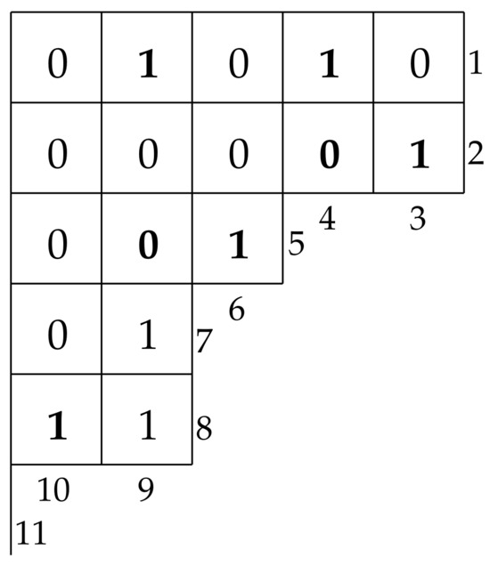
Figure 1. A permutation tableau T of length 11.

Linked partitions were first introduced by Dykema [3] in the study of the unsymmetrized T-transform in free probability theory. A linked partition of $\left[n\right]$ is a collection of nonempty subsets $B_1,B_2,\dots ,B_m$ of $\left[n\right]$, called blocks, such that the union of $B_1,B_2,\dots ,B_m$ is $\left[n\right]$, and any two distinct blocks are nearly disjoint. Two blocks $B_i$ and $B_j$ are said to be nearly disjoint if, for any $k\in B_i\cap B_j$, one of the following conditions holds:

(1)

$k=min\left(B_i\right),\left|B_i\right|>1$ and $k\ne min\left(B_j\right)$;

(2)

$k=min\left(B_j\right),\left|B_j\right|>1$ and $k\ne min\left(B_i\right)$.

The linear representation of a linked partition was defined by Chen, Wu, and Yan [4]. Given a linked partition $\tau$ of $\left[n\right]$, list n vertices in a horizontal line with labels $1,2,\dots ,n$. For any block, $B=\{i_1,i_2,\dots ,i_k\}$, where $k\ge 2$ and $i_1<i_2<\cdots <i_k$ draw an arc from $i_1$ to $i_j$ for $j=2,\dots ,k$. For $i<j$, we use a pair $(i,j)$ to represent an arc from i to j, and we call i and j the left-hand and right-hand endpoint of arc $(i,j)$, respectively. For the sake of convenience, we also adopt a linear representation to set partitions. Two arcs $(i_1,j_1)$ and $(i_2,j_2)$ form a crossing if $i_1<i_2<j_1<j_2$, and they form a nesting if $i_1<i_2<j_2<j_1$. The number of pairs of arcs forming a crossing (resp., nesting) in $\tau$ is defined as the crossing number (resp., nesting number) of $\tau$. We denote the crossing number and the nesting number of the linked partition $\tau$ by $cr\left(\tau \right)$ and $ne\left(\tau \right)$, respectively.

For example, the linear representation of linked partition $\tau =\{1,3,5\}\left\{2\right\}\{3,8\}\left\{4\right\}\{6,7\}$ is shown in Figure 2. There is only one crossing formed by arcs $(1,5)$ and $(3,8)$ and one nesting formed by arcs $(3,8)$ and $(6,7)$, i.e., $cr\left(\tau \right)=1$ and $ne\left(\tau \right)=1$.

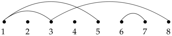
Figure 2. The linear representation of $\tau =\{1,3,5\}\left\{2\right\}\{3,8\}\left\{4\right\}\{6,7\}$.

Given a linked partition, a vertex in the linear representation of $\tau$ is called an origin if it is only a left-hand endpoint, a transient if it is both a left-hand point and a right-hand endpoint, a singleton if it is an isolated vertex, or a destination if it is only a right-hand endpoint. Figure 3 illustrates the four types of vertices. It is clear that origin, transition, and singleton are the minimum elements of the blocks, the total number of which is equal to the number of blocks of linked partitions. It should be pointed out that for any right-hand endpoint j, there is at most one vertex i such that $1\le i<j$, and i is connected to j in the linear representation of a linked partition.

Figure 3. Four types of elements in linked partitions.

Chen et al. [5] established a bijection between partitions and vacillating tableaux to prove that the crossing numbers and the nesting numbers of partitions of $\left[n\right]$ have a symmetric joint distribution by fixing the sets of minimal block elements and maximal block elements, as well as over all matchings on $\left[2n\right]$. They also obtained a corollary that the number of k-noncrossing partitions is equal to the number of k-non-nesting partitions, which is also true for matchings. Chen, Wu, and Yan [4] bijectively proved that the number of noncrossing linked partitions of $\left[n\right]$ is equal to the number of large Schröder paths of length $2(n-1)$, and they gave a one-to-one correspondence between linked partitions of $\left[n\right]$ and the increasing trees containing $n+1$ vertices. In addition, by defining linked cycles, they showed that the crossing number and nesting number have a symmetric joint distribution over the set of linked partitions of $\left[n\right]$ by fixing the vertex labeling. Chen, Liu, and Wang [6] gave a bijection between linked partitions of $\left[n\right]$ containing k blocks and permutations of $\left[n\right]$ containing $k-1$ descents, as well as a bijection between linked partitions of $\left[n\right]$ containing k blocks and permutation tableaux of length n containing k rows. Based on the positions of the topmost 1s and rightmost restricted 0s, they also defined $I_2$-avoiding and $J_2$-avoiding permutation tableaux. Moreover, they illustrated a bijection between noncrossing linked partitions of n and $J_2$-avoiding permutation tableaux of length n and a bijection between non-nesting linked partitions of n and $I_2$-avoiding permutation tableaux of length n. Chen, Guo, and Pang [7] introduced the structure of vacillating Hecke tableaux and used the Hecke insertion algorithm proposed by Buch et al. [8] to establish a one-to-one correspondence between vacillating Hecke tableaux and linked partitions; they also proved that the crossing number and the nesting number of a linked partition can be determined by the maximal number of rows and the maximal number of columns of diagrams in the corresponding vacillating Hecke tableau.

In this paper, we establish the relationship of internal structural characteristics between linked partitions and permutation tableaux. Especially, we present the crossing number and nesting number of linked partitions by the positional relationship between the topmost 1s and rightmost restricted 0s in permutation tableaux. For this target, we first introduce some new structual statistics of permutation tableaux in Section 2, such as the diagonal pattern, front-out condition, back-out condition, ceiling index, and floor index. In Section 3, we describe two marking algorithms for permutation tableaux in the view of columns and rows, respectively. In Section 4, we construct a tugging transformation and a rebound transformation to linked partitions, which show a closed relationship between set partitions and linked partitions: for any linked partition $\tau$ of n, there is a unique partition $\pi$ of n such that $\tau$ is generated by applying a tugging operation to $\pi$. Finally, based on the bijection between linked partitions and permutations, obtained by Chen, Liu, and Wang [6], we deduce that the crossing number and nesting number of a linked partition can be determined by the markers in the corresponding permutation tableau.

2. Structural Statistics in Permutation Tableaux

Let $PT\left(n\right)$ be the set of permutation tableaux of length n, where $n\ge 4$. Let $T\in PT\left(n\right)$, and denote its labels of columns by $j_1,j_2,\dots ,j_m$, where $j_1<j_2<\cdots <j_m,m\ge 2,n-m\ge 2$. A permutation tableau is uniquely determined by its topmost 1s and rightmost restricted 0s. The 1s and 0s we will mention next are both the topmost 1s and rightmost restricted 0s, abbreviated as $t.m.1$s and $r.r.0$s.

It can be fully proven that if the positions of the topmost 1s are given, then all the cells above these positions which are in the same columns are filled with 0s; if the positions of the rightmost restricted 0s are given, then all the cells to the left of these positions which are in the same rows are filled with 0s; and last, this fills the remaining cells with 1s.

Definition 1. 

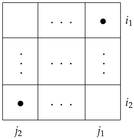
Two cells $(i_1,j_1)$ and $(i_2,j_2)$ in permutation tableau T form a diagonal pattern if $i_1<i_2<j_1<j_2$ and $(i_2,j_1)$ is a cell of T. See Figure 4.

Figure 4. Diagonal pattern.

For example, Figure 4 illustrates a diagonal pattern formed by cells $(i_1,j_1)$ and $(i_2,j_2)$, but cells $(2,4)$ and $(5,6)$ in Figure 1 cannot form a diagonal pattern, since the right of cell $(5,6)$ is empty without any cell.

For any column $j_a,1<a\le m$, denote the row label of its $t.m.1$ by $i_1$. Assume that there exists at least one $r.r.0$, and denote the row labels of all $r.r.0$s by $i_2,i_3,\dots ,i_k$, respectively, where $i_1<i_2<i_3<\cdots <i_k$, $2\le k\le n-m$.

Definition 2. 

We call $r.r.0$ in $(i_2,j_a)$ satisfying the front-out condition if there exist one $t.m.1$ or $r.r.0$s in cells $(i_1+1,j_b),(i_1+2,j_b),\dots ,(i_2-1,j_b)$,$1\le b\le a-1$, and $(i_2,j_b)$ is a cell of T. Figure 5 illustrates the condition for $j_b=j_{a-1}$.

Figure 5. The front-out condition.

Definition 3. 

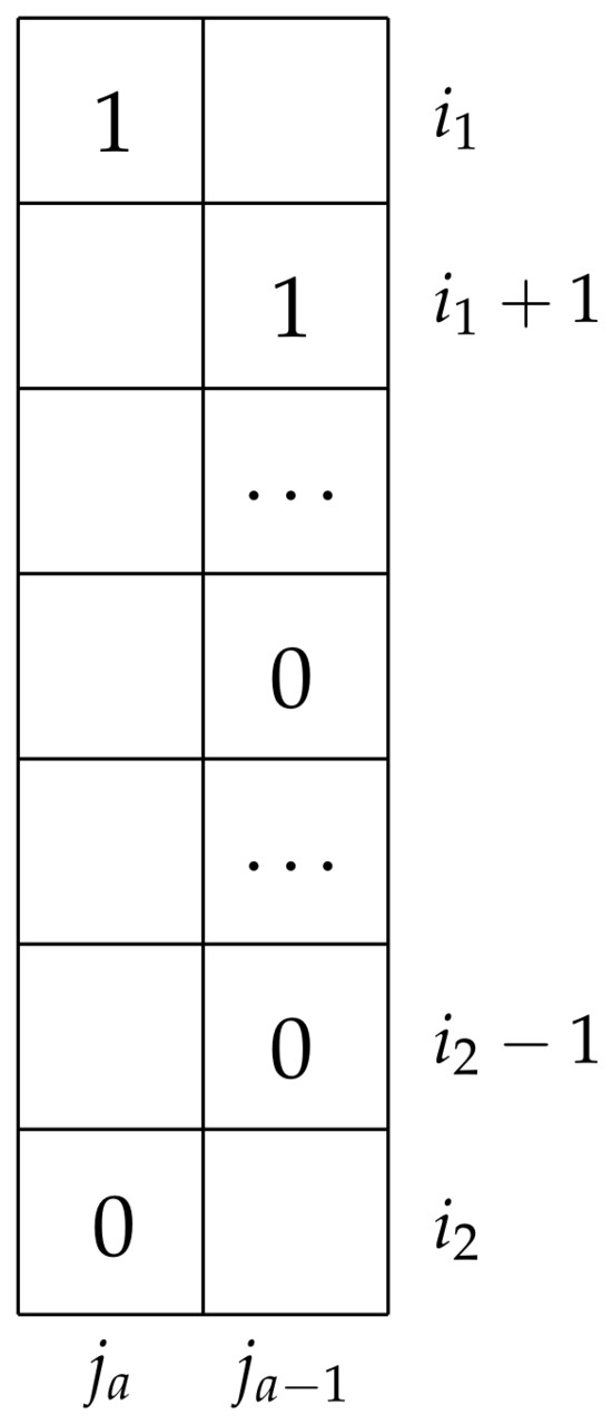
We call $r.r.0$ in $(i_2,j_a)$ satisfying the back-out condition if there exist a $t.m.1$ and possibly $r.r.0$s in cells $(i_1,j_b)$, $(i_1+1,j_b)$, …, $(i_2-1,j_b)$, $1\le b\le a-1$, and the cells meet one of the following conditions:

(a) 

There does not exist any $r.r.0$ under cell $(i_2,j_a)$ in column $j_a$, and $(i_2,j_{a-1})$ is a cell of T;

(b) 

There are $r.r.0$s under cell $(i_2,j_a)$ in column $j_a$ but cannot form a diagonal with $(t,j_{a-1})$, or t is the row label of the possible cells in column $j_{a-1}$, where $i_1\le t\le i_2-1$;

(c) 

There exists at least one cell filled with an $r.r.0$ in row i and column $j_b$, $i_2<i<i_3$, and cell $(i_3,j_{a-1})$ is in T.

Figure 6 illustrates the back-out condition when $j_b=j_{a-1}$.

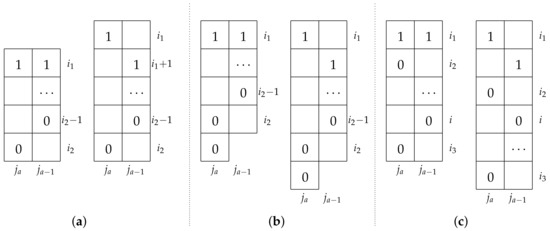
Figure 6. Six cases of the back-out condition. (a) Case 1, (b) Case 2, (c) Case 3.

Note that if the $r.r.0$ in cell $(i_2,j_a)$ satisfies the back-out condition, this means that only one of the three conditions above is met.

Definition 4. 

The ceiling index of any cell $(i,j)$ filled with a $t.m.1$ or an $r.r.0$ in T is defined as row label i.

Definition 5. 

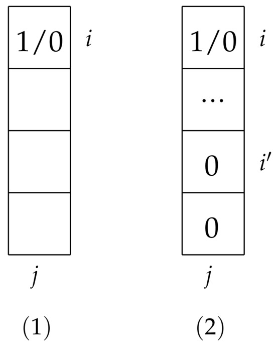
The floor index of cell $(i,j)$ filled with a $t.m.1$ or an $r.r.0$ in T is defined as column label j if there does not exist any $r.r.0$ below cell $(i,j)$ in column j; see Figure 7(1). Otherwise, its floor index is defined as row lable $i^{\prime }$ of cell $(i^{\prime },j)$, where cell $(i^{\prime },j)$ is filled with an $r.r.0$, $i^{\prime }>i$, and $|i^{\prime }-i|$ is minimum. See Figure 7(2).

Figure 7. Two cases of the floor index.

3. Marking Algorithms for Permutation Tableaux

In this section, we mainly introduce a marking algorithm and two statistics for permuatation tableaux called the row index and column index.

3.1. Column Marking Algorithm

Let T be a permutation tableau of length n with u rows and v columns, where $n\ge 4,v\ge 2$, and $n=u+v$. Denote the column labels of T by $j_1$, $j_2$, …, $j_v$, where $j_1<j_2<\cdots <j_v$. We introduce the column marking algorithm for permutation tableaux. We carry out the marking process to column $j_1$, $j_2$, …, $j_v$ in order, and we will mark some cells in these columns with one or some •s based on the positional relationship between actually present $r.r.0$s and $t.m.1$s in these columns.

For any column $j_a$, $1<a\le v$, we label its $t.m.1$ and possible $r.r.0$s by observing the positional relationships of $t.m.1$s and $r.r.0$s in column $j_a$ and columns $j_{a-1},j_{a-2},\dots ,j_1$, respectively.

Here, we take $j_a$ and $j_k$$(1\le k\le a-1)$ to illustrate the marking process of the $t.m.1$ and $r.r.0$s in $j_a$. Denote the row label of $t.m.1$ in column $j_a$ by $i_1$. First, if the $t.m.1$s in columns $j_a$ and $j_k$ form a diagonal pattern, then add a • in cell $(i_1,j_a)$. If there does not exist any $r.r.0$ in column $j_a$, we do nothing. Otherwise, assume that there is at least one $r.r.0$ in this column, and denote the row labels of those $r.r.0$s by $i_2,\dots ,i_f,i_1<i_2<\cdots <i_f$.

Second, we consider the mark of cell $(i_2,j_a)$. If there exist $t.m.1$ or $r.r.0$s in cells $(i_1+1,j_k),(i_1+2,j_k),\dots ,(i_2-1,j_k)$, i.e., the $r.r.0$ in cell $(i_2,j_a)$ satisfies the front-out condition, then add a • in cell $(i_2,j_a)$. If the $r.r.0$ in cell $(i_2,j_a)$ satisfies one of the back-out conditions, then add a • to cell $(i_2,j_a)$.

The number of •s in cell $(i_2,j_a)$ is called the column index of cell $(i_2,j_a)$ about column $j_k$, which is denoted by $C[(i_2,j_a);j_k]$. Next, we apply the same method to analyze the marks of cells $(i_3,j_a),(i_4,j_a),\dots ,(i_f,j_a)$, respectively, and obtain their column indices $C[(i_3,j_a);j_k]$, $C[(i_4,j_a);j_k]$, …, $C[(i_f,j_a);j_k]$. At this point, we have completed the column marking algorithm on column $j_a$ corresponding to column $j_k$.

By the same way, we apply the column marking algorithm to column $j_a$ corresponding to any column $j_k$, $k=a-2,\dots ,1$. Finally, the column marking algorithm of column $j_a$ is completed. Repeat the above process to the columns of T from $j_2$ to $j_v$. Then, the column marking algorithm for T is terminated.

Define

$$C\left[(i_2,j_a)\right]=\sum _{k=1}^{a-1}C[(i_2,j_a);j_k],C\left[j_a\right]=\sum _{t=1}^{f}C\left[(i_t,j_a)\right]$$

as the column index of cell $(i_2,j_a)$ and column $j_a$, respectively.

Definition 6. 

Let $\mathbb{N}$ be the set of non-negative integers and $\mathcal{Ƭ}$ be the set of permutation tableaux. Define a funciton F from $\mathcal{Ƭ}$ to $\mathbb{N}$ such that for any $T\in \mathcal{Ƭ}$,

$$F\left(T\right)=\sum _{q=2}^{v}C\left[j_q\right],$$

where the value of $F\left(T\right)$ is called the column index of T.

3.2. Row Marking Algorithm

Let T be a permutation tableau of length n with u rows and v columns, where $n\ge 4,v\ge 2$, and $n=u+v$. Denote the row labels of T by $i_1,i_2,\dots ,i_u,i_1<i_2<\cdots <i_u$. We carry out the marking process to row $i_2$, $i_3$, …, $i_u$ in order. Assume that there exists a cell $(i_b,j)$ containing a $t.m.1$ or an $r.r.0$ for any $1<b\le u$. According to Definition 4, its ceiling index is $i_b$, and we denote its floor index by t. If there exist exactly k cells in T filled with either a $t.m.1$ or an $r.r.0$, each of whose ceiling index is less than $i_b$ and floor index is greater than t, then add k ∗s to cell $(i_b,j)$, where $k\ge 0$. Define the row index of cell $(i_b,j)$ as k, which is denoted by $N\left[(i_b,j)\right]=k$.

Repeat the process for the other cells filled with either a $t.m.1$ or an $r.r.0$ in row $i_b$ and and obtain their row indices. Let $N\left[i_b\right]$ be the total number of ∗s in row $i_b$. After we obtain the row index of each row in T, the row marking algorithm for T is completed.

Definition 7. 

Let $\mathbb{N}$ be the set of non-negative integers and $\mathcal{Ƭ}$ be the set of permutation tableaux. Define a funciton G from $\mathcal{Ƭ}$ to $\mathbb{N}$ such that for any $T\in \mathcal{Ƭ}$,

$$G\left(T\right)=\sum _{b=2}^{u}N\left[i_b\right],$$

where the value of $G\left(T\right)$ is called the row index of T.

3.3. An Example

Here, we provide an example to further illustrate the two algorithms discussed above. Let $T_1$ be the permutation tableau in Figure 8. First, let us apply the column marking algorithm on $T_1$.

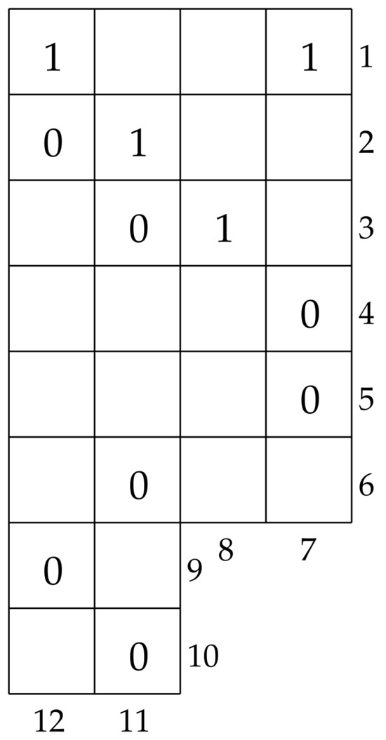
Figure 8. A permutation tableau $T_1$ of length 12.

According to the column marking algorithm, we possibly mark the cells containing $t.m.1$s and $r.r.0$s in columns $8,11,12$ from right to left in order.

For column 8, we only add a • to cell $(3,8)$, since the 1s in cells $(3,8)$ and $(1,7)$ form a diagonal pattern. Let $C\left[\right(3,8);7]=1$; see Figure 9(1). For columns 11 and 8, firstly note that cell $(6,11)$ satisfies the back-out condition, so add a • to the cell and let $C\left[\right(6,11);8]=1$. For columns 11 and 7, cells $(2,11)$ and $(1,7)$ form a diagonal pattern, where this implies that $C\left[\right(2,11);7]=1$. Because cell $(6,11)$ satisfies both the front-out condition and the back-out condition, add two •s to $(6,11)$ and obtain $C\left[\right(6,11);7]=2$. See Figure 9(2). Similarly, for column 12, we have $C\left[\right(9,12);11]=2,C\left[\right(2,12);7]=1$. See Figure 9(3). Finally, we obtain

$$\begin{array}{cc}\hfill F\left(T_1\right)& =C\left[7\right]+C\left[8\right]+C\left[11\right]+C\left[12\right]\hfill \\ \hfill & =0+C\left[\right(3,8);7]+\left(C\right[(6,11);8]+C[(2,11);7]+C[(6,11);7\left]\right)\hfill \\ \hfill & +\left(C\right[(9,12);11]+C[(2,12);7\left]\right)\hfill \\ \hfill & =0+1+4+3\hfill \\ \hfill & =8.\hfill \end{array}$$

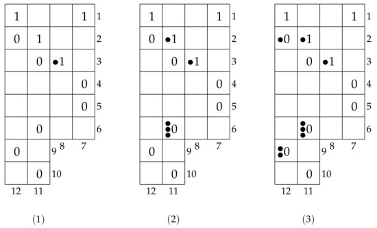
Figure 9. The column marking algorithm of $T_1$.

On the other hand, we carry out the row marking algorithm on $T_1$. According to the row marking algorithm, we possibly mark the cells containing $t.m.1$s and $r.r.0$s in rows $2,3,4,5,6,9,10$ from top to bottom in order. For row 2, we just add an ∗ to cell $(2,11)$, becasue its ceiling index is 2, which is greater than the ceiling index of $(1,7)$, and its floor index is 3, which is less than the floor index of $(1,7)$. Let $N\left[\right(2,11);1]=1$. See Figure 10$\left(1\right)$. Similarly, for row 3, add one ∗ to $(3,11)$, and add one ∗ to $(3,8)$. Note that $N\left[\right(3,11);2]=1$, and $N\left[\right(3,8);2]=1$; see Figure 10(2). For row 4, add three ∗s to $(4,7)$, and let $N\left[\right(4,7);2]=1$ and $N\left[\right(4,7);3]=2$; see Figure 10(3). For row 5, add two ∗s to $(5,7)$. Note that $N\left[\right(5,7);2]=1$, and $N\left[\right(5,7);3]=1$; see Figure 10(4). Row 6 and 9 do not satisfy the row marking condition and are not marked. For row 10, add one ∗ to $(10,11)$, and let $N\left[\right(10,11);9]=1$; see Figure 10(5). Finally, we obtain

$$\begin{array}{cc}\hfill G\left(T_1\right)& =N\left[1\right]+N\left[2\right]+N\left[3\right]+N\left[4\right]+N\left[5\right]+N\left[6\right]+N\left[9\right]+N\left[10\right]\hfill \\ \hfill & =0+N\left[\right(2,11);1]+\left(N\right[(3,8);2]+N[(3,11);2\left]\right)+\left(N\right[(4,7);2]+N[(4,7);3\left]\right)\hfill \\ \hfill & +\left(N\right[(5,7);2]+N[(5,7);3\left]\right)+0\hfill \\ \hfill & +0+N\left[\right(10,11);9]\hfill \\ \hfill & =0+1+2+3+2+0+0+1\hfill \\ \hfill & =9.\hfill \end{array}$$

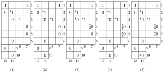
Figure 10. The row marking algorithm of $T_1$.

4. Transformations on Linked Partitions

In this section, we introduce two transformations on linked partitions, called tugging and rebound, and a recursive generating procedure.

Definition 8. 

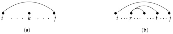
For a linked parition τ, if there exist a singleton k and an arc $(i,j)$ such that $i<k<j$, then we call k a tuggable singleton of arc $(i,j)$, as shown in Figure 11a. If there exist an origin r, a destination t, and an arc $(i,j)$ such that $i<r<t<j$, where both r and t are contained in the same block B and $t=max\left(B\right)$, then we call r a tuggable origin of arc $(i,j)$, as shown in Figure 11b.

Figure 11. Different types of tuggable vertices.

Both tuggable singletons and tuggable origins are called tuggable vertices. Arc $(i,j)$ is called a tuggable arc.

Definition 9. 

If there exist arcs $(i,j)$ and $(i^{\prime },j^{\prime })$ satisfying $i^{\prime }\le i<j<j^{\prime }$, then we say that arc $(i^{\prime },j^{\prime })$ covers arc $(i,j)$. The number of arcs covering arc $(i,j)$ is called the level of arc $(i,j)$, which is denoted by ${\ell }_{(i,j)}$.

Definition 10. 

For any arcs $(i,j)$ and $(i^{\prime },j^{\prime })$, if ${\ell }_{(i,j)}>{\ell }_{(i^{\prime },j^{\prime })}$ or ${\ell }_{(i,j)}={\ell }_{(i^{\prime },j^{\prime })}$ but $i<i^{\prime }$, then we consider arc $(i,j)$ as having a higher level than arc $(i^{\prime },j^{\prime })$, which is denoted by $(i,j)\succ (i^{\prime },j^{\prime })$. We call $\alpha =[{\alpha }_1,{\alpha }_2,\dots ,{\alpha }_k]$ the arc sequence of τ if the ${\alpha }_t$s are all its arcs, $1\le t\le k$, and ${\alpha }_1\succ {\alpha }_2\succ \cdots \succ {\alpha }_k$.

For example, as shown in Figure 2, linked parition $\tau$ has two tuggable singletons 2 and 4 and a unique tuggable origion 6. Moreover, ${\ell }_{(1,3)}={\ell }_{(6,7)}=1$ and $(1,3)\succ (6,7)$; likewise, ${\ell }_{(1,5)}={\ell }_{(3,8)}=0$ and $(1,5)\succ (3,8)$. So, the arc sequence of $\tau$ is

$$\alpha =[{\alpha }_1,{\alpha }_2,{\alpha }_3,{\alpha }_4]=[(1,3),(6,7),(1,5),(3,8)].$$

Definition 11. 

Given a linked parition of τ, if there exists a tuggable vertice k of any arc $(i,j)$, then we remove arc $(i,j)$ from τ and add arcs $(i,k)$ and $(k,j)$. Denote the resulting graph by ${\tau }^{\prime }$. The transformation from τ to ${\tau }^{\prime }$ is denominated as a tugging operation on arc $(i,j)$ at vertice k.

${\tau }^{\prime }$ is a linked partition because each vertex is a right-hand endpoint of at most one arc. The procedure of carrying out the tugging operation on arcs at any one of the tuggable vertices in $\tau$ or doing nothing is called a tugging transformation to $\tau$. Note that k is a transition of ${\tau }^{\prime }$, that is to say, it must not be a tuggable vertex of ${\tau }^{\prime }$.

As illustrated in Figure 12, ${\tau }_1$ is obtained from performing a tugging transformation to $\tau$ in Figure 2: firstly, we tug arc $(1,3)$ at tuggable singleton 2, tug arc $(1,5)$ at tuggable singleton 4, and finally do nothing for arc $(3,8)$; however, 6 is its tuggable origin.

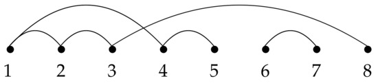
Figure 12. The result ${\tau }_1$ of performing tugging transformations to $\tau$.

Next, we introduce the inverse transformation of tugging transformation for linked partitions.

Definition 12. 

Given a linked parition of ${\tau }^{\prime }$, suppose there exists a transition k connecting arcs $(i,k)$ to $(k,j)$, where both k and j are in block B, $k=min\left(B\right)$, and $j=max\left(B\right)$; we remove arcs $(i,k)$ and $(k,j)$ from ${\tau }^{\prime }$ while adding arc $(i,j)$. Denote the resulting graph by ${\tau }^{″}$. The transformation from ${\tau }^{\prime }$ to ${\tau }^{″}$ is denominated as a rebound operation on arcs $(i,k)$ and $(k,j)$ at transition k.

It is not difficult to find that ${\tau }^{″}$ is also a linked partition. The procedure of performing a single rebound operation on arcs at any one of transitions in a linked partition or doing nothing is called a rebound transformation to $\tau$. As illustrated in Figure 13, ${\tau }_2$ is obtained from performing rebound transformations to ${\tau }_1$ in Figure 12 at transitions 2, 3, and 4 in order.

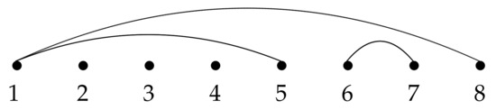
Figure 13. The result ${\tau }_2$ of performing rebound transformation to ${\tau }_1$.

The tugging procedure is the way to perform the tugging transformation to set partitions of $\left[n\right]$, thus giving linked partitions a nice recursive structure. Next, we define this tugging procedure, and we present a generation table for linked partitions.

A set partition $\pi$ of $\left[n\right]$ is a collection of disjoint nonempty subsets of $\left[n\right]$, that is,

$$\pi =\left\{B_1,B_2,\dots ,B_m\right\},$$

where the $B_i$s are called blocks, $i=1,2,\dots ,m$, and whose union is $\left[n\right]$.

We adopt the same linear representation for set partitions. Given that $\pi$ is a set partition of $\left[n\right]$, i.e., $\pi$ does not have any transition, then we perform the tugging transformation to $\pi$ once. The result ${\pi }^{\prime }$ satisfies that either ${\pi }^{\prime }=\pi$ or ${\pi }^{\prime }$ is a linked partition, and it has its own possible tuggable vertex. We could repeat the above process for ${\pi }^{\prime }$. Furthermore, given set partitions ${\pi }_1$, ${\pi }_2$, and ${\pi }_1\ne {\pi }_2$, exerting a tugging transformation on ${\pi }_1$ and ${\pi }_2$, respectively, the result of linked partitions ${\pi }_1^{\prime }$ and ${\pi }_2^{\prime }$ must be different from each other.

On the contraty, given a linked partition $\tau$, we can obtain set partitions by exerting rebound transformations at all of the transitions. Thus, the following conclusion is provided.

Theorem 1. 

Any linked partition of $\left[n\right]$ can be produced from some set partition of $\left[n\right]$ by means of a tugging transformation.

In Figure 14, we demonstrate that linked partitions of $\{1,2,3,4\}$ can be generated from the set partitions of $\{1,2,3,4\}$. It is evident that linked partitions with labels $b,c$, and d are generated from the same set partition with label a, repectively; on the other hand, when applying the tugging transformation to the set partition with label a by considering different tuggable verices or doing this once or twice, we obtain different linked partitions. It implies that there does not exist any bijective correspondence between the set of linked partitions of $\left[n\right]$ and the set of set partitions of $\left[n\right]$, but we can construct all of the linked partitions based on the set partitions.

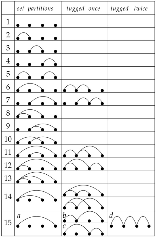
Figure 14. Generating table of linked partitions of $\{1,2,3,4\}$.

5. Main Theorem

Review that Chen, Liu, and Wang [6] proved a bijection $\phi$ between linked partitions and permutation tableaux. Combining bijection $\phi$ with marking algorithms, we are led to the main result that $cr\left(\tau \right)$ and $ne\left(\tau \right)$ in any linked partition $\tau$ can be indicated by a linear function of the number of different markers in $\phi \left(\tau \right)$.

Theorem 2 

(Chen, Liu, and Wang [6]). For $n\ge 1$ and $1\le k\le n$, there is a bijection φ between a linked partition of $\left[n\right]$ with k blocks and a permutation tableau T of length n with k rows.

Here, we review the map $\phi$ from permutation tableaux to linked partitions. Let $T\in PT\left(n\right)$. After that, let us construct a linked partition $\tau$ of $\left[n\right]$ such that $T=\phi \left(\tau \right)$. First, we draw n vertices in a horizontal line labeled by $1,2,\dots ,n$ from left to right; for any $k=1,2,\dots ,m$, we connect vertex $i_k$ to $i_{k+1}$ with an arc, where $i_{m+1}=j$. For the column labeled with j, let $(i_1,j)$ be the cell filled with a $t.m.1$, and let $(i_2,j),(i_3,j),\dots ,(i_m,j)$ be the cells filled with the $r.r.0$s. Afterwards, repeat the above process for all columns. Then, we have the desired linked partition.

For example, the linked partition ${\tau }_1$ corresponding to the bijective relationship with the permutation tableaux $T_1$ in Figure 8 is shown as follows.

Then, it is not difficult to have the following result.

Proposition 1. 

Let τ be a linked partition and $T=\phi \left(\tau \right)$ be the correspending permutation tableau:

(1)

If τ is a set partition, then there does not exist any $r.r.0$ in T.

(2)

If there exists a tuggable vertex k of an arc $(i,j)$ in τ, then performing the tugging transformation to k is equivalent to adding an $r.r.0$ to cell $(k,j)$ of T.

Furthermore, based on Theorem 1 and the definition of permutation tableaux, we have the following theorems.

Theorem 3. 

Permutation tableaux of length n can be generated from the permutation tableaux containing just $t.m.1$s by doing nothing or adding $r.r.0$s in the cells satisfying the following three conditions simultaneously:

(a) 

The $r.r.0$s can only be added below the $t.m.1$s.

(b) 

There does not exist any $r.r.0$ with $t.m.1$s above (in the same column) and a $t.m.1$ to the left (in the same row).

(c) 

Each row contains only one $r.r.0$.

Based on the bijection $\phi$ between linked paritions and permutation tableaux in Theorem 2, we have the following conclusion.

Theorem 4. 

Let τ be a linked partition of $\left[n\right]$ and $cr\left(\tau \right)=m$, where $ne\left(\tau \right)=\ell$. If permutation tableau $T=\phi \left(\tau \right)$, then $F\left(T\right)=m$, and $G\left(T\right)=\ell$.

The interpretation of bijection $\phi$ implies that applying the tugging transformation to some arcs in a linked partition $\tau$ corresponds to the process of adding $r.r.0$s in permutation tableau $T=\phi \left(\tau \right)$. Moreover, judging whether certain cells meet the front-out condition, the back-out condition, or from a diagonal pattern in T, we determine whether a new crossing is generated after tugging an arc in $\tau$. Comparing the size relationship between the ceiling index and the floor index of two cells in T determines whether the corresponding arcs in $\tau$ form a nesting or not. Then by applying the column and row marking algorithm in T, respectively, one can thoroughly identify the crossings and nestings in $\tau$ and finally obtain $cr\left(\tau \right)$ and $ne\left(\tau \right)$ from the total numer of •s and ∗s. Hence, we have the desired theorem.

There is a bijection between ${\tau }_1$ shown in Figure 15 and $T_1$ shown in Figure 8. It is not difficult to comprehend that $cr\left({\tau }_1\right)$ = 8 and $ne\left({\tau }_1\right)$ = 9. Based on the row and column marking algorithms of the permutation tableaux, we know that $G\left(T_1\right)$ = 9 and $F\left(T_1\right)$ = 8. As stated in our Theorem 4, we understand that $F\left(T_1\right)$ = $cr\left({\tau }_1\right)$ and $G\left(T_1\right)$ = $ne\left({\tau }_1\right)$.

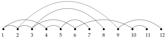
Figure 15. The linear representation of ${\tau }_1=\{1,2,4\}\{2,3,9\}\{3,6,8\}\{4,5\}\{5,7\}\{6,10\}\{9,12\}\{10,11\}$.

References

- Steingrímsson, E.; Williams, L. Permutation tableaux and permutation patterns. J. Combin. Theory Ser. A 2007, 114, 211–234. [Google Scholar] [CrossRef][Green Version]
- Corteel, S.; Kim, J.S. Combinatortics on permutation tableaux of type A and type B. Eur. J. Comb. 2011, 32, 563–579. [Google Scholar] [CrossRef][Green Version]
- Dykema, K.J. Multilinear Function Series and Transforms in Free Probability Theory. Adv. Math. 2007, 208, 251–407. [Google Scholar] [CrossRef]
- Chen, W.Y.C.; Wu, S.Y.J.; Yan, C.H. Linked Partitions and Linked Cycles. Eur. J. Comb. 2008, 29, 1408–1426. [Google Scholar] [CrossRef]
- Chen, W.Y.C.; Deng, E.Y.P.; Du, R.R.X.; Stanley, R.P.; Yan, C.H. Crossings and nestings of matchings and partitions. Trans. Am. Math. Soc. 2007, 359, 1555–1575. [Google Scholar] [CrossRef]
- Chen, W.Y.C.; Liu, L.H.; Wang, C.J. Linked Partitions and Permutation Tableaux. Electron. J. Comb. 2013, 20, 1823–1831. [Google Scholar] [CrossRef] [PubMed]
- Chen, W.Y.C.; Guo, P.L.; Pang, S.X.M. Vacillating Hecke Tableaux and Linked Partitions. Math. Z. 2015, 281, 661–672. [Google Scholar] [CrossRef]
- Buch, A.S.; Kresch, A.; Shimozono, M.; Tamvakis, H.; Yong, A. Stable Grothendieck polynomials and K-theoretic factor sequences. Math. Ann. 2008, 340, 359–382. [Google Scholar] [CrossRef][Green Version]
Disclaimer/Publisher’s Note: The statements, opinions and data contained in all publications are solely those of the individual author(s) and contributor(s) and not of MDPI and/or the editor(s). MDPI and/or the editor(s) disclaim responsibility for any injury to people or property resulting from any ideas, methods, instructions or products referred to in the content. |
© 2025 by the authors. Licensee MDPI, Basel, Switzerland. This article is an open access article distributed under the terms and conditions of the Creative Commons Attribution (CC BY) license (https://creativecommons.org/licenses/by/4.0/).