Flexible Job Shop Dynamic Scheduling and Fault Maintenance Personnel Cooperative Scheduling Optimization Based on the ACODDQN Algorithm

Abstract

In order to address the impact of equipment fault diagnosis and repair delays on production schedule execution in the dynamic scheduling of flexible job shops, this paper proposes a multi-resource, multi-objective dynamic scheduling optimization model, which aims to minimize delay time and completion time. It integrates the scheduling of the workpieces, machines, and maintenance personnel to improve the response efficiency of emergency equipment maintenance. To this end, a self-learning Ant Colony Algorithm based on deep reinforcement learning (ACODDQN) is designed in this paper. The algorithm searches the solution space by using the ACO, prioritizes the solutions by combining the non-dominated sorting strategies, and achieves the adaptive optimization of scheduling decisions by utilizing the organic integration of the pheromone update mechanism and the DDQN framework. Further, the generated solutions are locally adjusted via the feasible solution optimization strategy to ensure that the solutions satisfy all the constraints and ultimately generate a Pareto optimal solution set with high quality. Simulation results based on standard examples and real cases show that the ACODDQN algorithm exhibits significant optimization effects in several tests, which verifies its superiority and practical application potential in dynamic scheduling problems.

1. Introduction

With the accelerated transformation of global manufacturing into automation and intelligence, the Flexible Job Shop Problem [1] (FJSP) has become an important research direction in the field of production management optimization. The deep integration of the new generation of information technology, especially cloud computing [2], the Internet of Things [3], digital twin [4], and other key technologies, has driven manufacturing systems to a high degree of automation and flexibilization [5]. However, the traditional static flexible job shop scheduling model faces many dynamic challenges in practical applications, mainly including random arrivals and process changes at the order level, abnormal disturbances and parameter fluctuations at the equipment level, and real-time response requirements at the system level. In a dynamic environment, the traditional FJSP model often shows limitations regarding response lag and optimization failure, which makes it challenging to meet the demand for efficient scheduling in modern manufacturing systems. Therefore, the dynamic scheduling of flexible job shops (DFJSP) [6] problem has gradually become a key research topic in the field of intelligent manufacturing.

The flexible job shop scheduling problem (FJSP) has been studied extensively before, covering a wide range of types such as standard FJSPs, distributed FJSPs, and uncertain FJSPs. These studies usually decompose the FJSP into two main subproblems, namely operation sequence (OS) and machine assignment (MA) [7]. Existing studies show that the main optimization objectives of the FJSP are mainly focused on minimizing completion time. However, the traditional optimization objectives are often challenging to meet due to the complexity of the actual production environment, so the study of dynamic FJSP (DFJSP) problems with multiple resource constraints and multi-objective optimization is of great significance [8]. In recent years, scholars have conducted in-depth research on the dynamic scheduling problem of multi-objective flexible job shops and proposed a variety of optimization methods. For example, Yue et al. [9] proposed a two-stage double-depth Q-network (TS-DDQN) algorithm to solve the dynamic scheduling problem that includes new workpiece insertion and machine failures, aiming to optimize the total delay time and machine utilization; Zhang et al. [10] designed a two-stage algorithm based on a convolutional network for the study of the dynamic flexible job shop scheduling problem that takes into account machine failures, aiming to optimize completion time minimization and improve scheduling robustness; Gao et al. [11] combined the improved Jaya algorithm with local search heuristics to optimize the re-scheduling process of DFJSP, which achieves the minimization of completion time and the improvement of scheduling stability; Luan et al. [12] proposed an improved chimpanzee optimization algorithm for solving a multi-objective flexible job shop scheduling problem; Lv et al. [13] used the AGE- MOEA algorithm to solve a dynamic scheduling problem under emergency order insertion and multiple machine failures, optimizing completion time and total energy consumption; and Yuan et al. [14] used a deep reinforcement learning algorithm to solve a multi-objective dynamic flexible job shop scheduling problem considering the insertion of new workpieces, and achieved the minimization of multiple objectives such as completion time.

With the depth of research, scholars have gradually come to recognize the important role of human factors in production scheduling; especially in the complex dynamic scheduling environment, the synergy between human and machine resources is crucial to optimizing the scheduling performance. Therefore, incorporating human factors into the scheduling system can not only construct a more accurate and comprehensive scheduling model, but also improve the robustness of rescheduling, thus effectively improving production management efficiency [15]. Based on this, some scholars have begun to explore the multi-objective flexible job shop dynamic scheduling (DFJSP) problem involving the dual resources of humans and machines. For example, Zhang et al. [16] used an improved non-dominated sorting genetic algorithm (INSGA-II) to solve the energy-saving optimization problem of a flexible job shop considering both machine and worker scheduling and the optimization objectives, including the total energy consumption, completion time, and delay time; Li et al. [17] proposed a genetic algorithm based on the Improved Hybridized Producer–Consumer Framework (IPFGA) for solving a multi-objective DFJSP problem that considers the workers’ scheduling. Scheduling: Sun et al. [18] proposed a two-level nested Ant Colony Algorithm for the DFJSP problem involving both worker and machine tool scheduling to optimize the quality of critical jobs and minimize completion time; Mokhtari et al. [19] used a hybrid artificial bee colony (HABCO) algorithm to study the human–computer interface. Although existing studies have considered the factors of worker scheduling, few studies have delved into the problem of scheduling maintenance personnel after a machine failure, especially in dynamic scheduling scenarios, where the occurrence of machine failures often leads to significant changes in the production scheduling plan, and the timely response and reasonable scheduling of the maintenance personnel are of great importance for production recovery.

In terms of solution methods for the dynamic scheduling problem of flexible job shops, the current research focuses on two main categories: local search heuristic algorithms and meta-heuristic algorithms [20]. Local search heuristic algorithms, such as Variable Neighborhood Search (VNS) and Taboo Search (TS), optimize the quality of the solution through neighborhood search, while meta-heuristic algorithms, such as the Genetic Algorithm (GA), Particle Swarm Optimization (PSO), Artificial Bee Colony Algorithm (ABC), and Ant Colony Optimization (ACO) Algorithm, carry out a global search to enhance the scheduling optimization effect through the mechanism of group intelligence or bio-inspiration [21]. Due to the powerful global search capability of meta-heuristic algorithms, they have been widely used to solve DFJSP problems. Long et al. [22] proposed a self-learning artificial bee colony (SLABC) algorithm for solving dynamic scheduling problems considering job insertion; Chen et al. [23] proposed a modified Ant Colony Optimization (PACO) Algorithm for solving the DFJSP problem; and Liang et al. [24] devised a genetic algorithm (GA) to cope with the dynamic scheduling problem considering machine failure interference. Although these heuristic-based algorithms have been successful to a certain extent, with the increasing complexity of the flexible job shop scheduling problem, mainly when multiple resources and multiple objectives are involved, the traditional algorithms can hardly satisfy the demand of intelligent production in terms of solution rate and accuracy. Therefore, it is imperative to explore more efficient algorithms to cope with complex dynamic scheduling problems.

In recent years, deep reinforcement learning (DRL) has been widely applied to solve DFJSP problems as an optimization method with high potential. For example, Chen et al. [25] used the Rainbow Deep Q-Network (Rainbow DQN) to solve a flexible job shop dynamic scheduling problem considering shop floor heterogeneity and workpiece insertion, aiming to minimize the total weighted delay and total energy consumption; Peng et al. [26] designed a two-stage Efficient Modulo Algorithm (EMA) for solving a distributed job shop scheduling problem with flexible machining time, which resulted in the minimization of energy consumption and processing time; Su et al. [27] proposed a graph reinforcement learning (GRL) approach to solve the multi-objective flexible job shop scheduling problem (MOFJSP) and generated a high-quality Pareto solution set by decomposing the multi-objective problem into different sub-problems based on preferences; and Liu et al. [28] used an actor-critic reinforcement learning algorithm to solve job shop scheduling problems. Wang et al. [29] used the PPO algorithm to solve the dynamic job shop scheduling problem considering machine failures and workpiece reworking; Luo et al. [30] constructed a bi-hierarchical deep Q-network (THDQN), which solves the complex and variable dynamic job shop scheduling problem and optimizes the average utilization rate of the machine and the total tardiness rate; Liu et al. [31] used a two-loop deep Q-network approach to solve a flexible job shop dynamic scheduling problem considering emergency order insertion; Palacio et al. [32] used a Q-learning algorithm to optimize a real manufacturing scenario of assembling light switches, achieving the goal of Makespan minimization; Gui et al. [33] used the DDPG algorithm to train a policy network, compounding a single dispatch rule into an optimal dispatch rule and solving for the average machine utilization and lateness; Zhang et al. [34] designed a dual two-depth Q-network algorithm to solve the dynamic scheduling problem of a flexible job shop with consideration of transportation time. Although deep reinforcement learning (DRL) has made some progress in the dynamic scheduling of flexible job shops, the algorithms face efficiency and accuracy challenges when dealing with complex scheduling problems. Therefore, this paper proposes an innovative scheduling method combining deep reinforcement learning and heuristic algorithms, aiming to solve multi-objective, multi-resource, and human–machine collaborative scheduling problems and provide an efficient solution for dynamic scheduling in intelligent production. Table 1 summarizes the differences between the above studies and this study.

Table 1. Summary of the existing literature.

Work	State	Dynamic Event	Objective	Algorithm	Problem
Chen et al. (2024) [25]	Discrete	Job random arrival	Total tardiness; Total energy consumption	Rainbow DQN	FJSP
Peng et al. (2025) [26]	Discrete	Random processing time; Variable production	Makespan; Total energy consumption	Efficient meme algorithm (EMA)	FJSP
Su et al. (2024) [27]	Discrete	Random processing time	Makespan; Maximum load; Machine workload	GRL	FJSP
Liu et al. (2020) [28]	Discrete	Machine breakdowns; Random processing time	Makespan	Deep deterministic policy gradient	JSP
Wang et al. (2021) [29]	Discrete	Machine breakdowns; Random processing time	Makespan	PPO	JSP
Luo et al. (2021) [30]	Continuous	Random job insertion	Makespan; Total tardiness; Average machine utilization	THDQN	JSP
Liu et al. (2020) [31]	Discrete	Machine breakdowns; Emergency Orders	Makespan	Actor-Critic	JSP
Palacio et al. (2022) [32]	Discrete	Machine breakdowns; Emergency Orders	Makespan	Q-learning	JSP
Gui et al. (2023) [33]	Continuous	Random processing time; Job random arrival	Mean tardiness	Deep deterministic policy gradient	FJSP
Zhang et al. (2024) [34]	Discrete	Job random arrival	Mean tardiness	Dueling double-depth Q-network	FJSP
This paper	Continuous	Job random arrival; Random processing time; Machine breakdowns	Minimum tardiness; Makespan	ACODDQN	FJSP

In this paper, the ACO and DDQN algorithms are combined to propose an efficient method to solve the multi-resource and multi-objective flexible job shop dynamic scheduling problem (MMO-DFJSP), namely the Adaptive Ant Colony Algorithm based on reinforcement learning (ACODDQN). The algorithm combines the global search capability of the Ant Colony Optimization (ACO) Algorithm with the adaptive learning characteristics of the double-depth Q-network (DDQN), aiming to cope with the scheduling optimization problem in complex dynamic environments, so as to achieve the dual minimization of delay time and completion time. Specifically, the main contributions of this paper include (1) constructing a multi-resource, multi-objective dynamic scheduling optimization model covering workpieces, machines, and maintenance personnel, which entirely takes into account the complexity of the production system and achieves the minimization of both delay time and completion time; (2) designing four kinds of composite scheduling rules based on workpieces, machines, and maintenance personnel, which improve the flexibility of the scheduling scheme through adaptive scheduling strategies and enhance the ability to cope with complex production environments. (3) A self-learning Ant Colony Algorithm based on deep reinforcement learning (ACODDQN) is proposed, which combines the global search capability of the Ant Colony Optimization (ACO) Algorithm with the intelligent decision-making mechanism of the double-depth Q-network (DDQN), significantly improves the algorithm’s adaptivity and optimization capability in dynamic scheduling problems, and provides more efficient scheduling decision support for complex production systems.

The rest of the paper is organized as follows: Section 2 describes the multi-objective flexible job shop dynamic scheduling problem and constructs a mathematical model. Section 3 introduces the ACODDQN algorithm. Section 4 analyzes the extended calculus further and provides examples using the algorithm. Section 5 concludes the paper.

2. Problem Description and Model Construction

2.1. Problem Description

The multi-constrained flexible job shop dynamic scheduling problem can be described as follows: the job shop has $n$ workpieces, $m$ machines, and $w$ maintenance personnel; each workpiece contains $n_i$ processes; each process has the corresponding machinable machine set and the corresponding processing time set; the ability of each maintenance personnel is different; and the time used for fault maintenance of the same machine is also different. Maintenance activities should not be interrupted during machine processing, and processing activities should not be carried out while maintenance is in progress. Under the conditions of workpiece constraint, machine constraint, and maintenance personnel constraint, the optimal machine combination is determined for each workpiece, and the most suitable maintenance personnel is assigned to the faulty machine.

The multi-constrained, multi-objective dynamic scheduling problem is studied based on workpiece, machine, and maintenance personnel. The research goal is to minimize the completion and delay times. In order to better solve the problem, the following hypotheses are given:

(1)

All workpieces, machines, and workers are available at 0;

(2)

There are order constraints between the operations of a job;

(3)

Maintenance personnel for different machine fault maintenance times is known;

(4)

At the same time, a machine can only process one process, and a maintenance worker can only carry out one maintenance activity;

(5)

Once started, unless machine failure occurs, no interruption is allowed until the operation is complete;

(6)

When the machine fails, the machine will be shut down immediately;

(7)

The repair time of the damaged machine is known;

(8)

The machine processing and maintenance process cannot be interrupted;

(9)

Do not consider transport time in the workpiece processing.

2.2. Model Establishment

The parameter settings are shown in Table 2. The mathematical model of MMO-DFJSP is established as follows.

Table 2. Main variables.

Notation	Description
Indexes:
$i$	Job index, $i$ $\mathsf{\in }$ {1,2,…,$n$}
$j$	Operational index, $j$ $\mathsf{\in }$ {1,2,…,$n_i$}
$k$	Machine index, $k$ $\mathsf{\in }$ {1,2,…,$m$}
$w$	Maintenance personnel index, $w$ $\mathsf{\in }$ {1,2,…,$q$}
Parameters:
$n$	Total number of jobs
$m$	Total number of machines
$n_i$	Number of operations of job $i$
$q$	Number of maintenance personnel
$J_i$	The $i^{th}$ job
$O_{ij}$	The $j^{th}$ operation of job $J_i$
$(t_{ij}^k{)}_s$	Process $O_{ij}$ machining start time of machine $k$
${(t_{ij}^k)}_f$	Procedure $O_{ij}$ machining end time of machine $k$
$t_{ij}$	Processing time of the workpiece $O_{ij}$
${{(t}_w^k)}_s$	Maintenance worker $w$ at the beginning of machine $k$ maintenance
${{(t}_w^k)}_f$	Maintenance worker $w$ at the end of machine $k$ maintenance
$t_w^k$	Time required for maintenance personnel $w$ to repair machine $k$
$p_k$	Last time machine $k$ can be processed
$m_k$	Machine $k$ last serviceable time
$m_w$	Worker $w$ recent repairable moments
$T_k$	Machine $k$ continuous working time
$C$	Production cycle time
$D_i$	Deadline completion time of job $i$
$D{T}_i$	Delay time of job $i$
$C_i$	Completion time of job $i$
$U{P}_i$	Urgency of job $i$, $U{P}_i$ ∈ [1,3]
Decision variables:
$X_{ijpsk}$	1 if machine $k$ preferentially process operation $O_{ij}$ and 0 otherwise
$X_{wkg}$	1 if Maintenance worker $w$ repairs machine $k$ first and 0 otherwise
$X_{ijk}$	1 if operation $O_{ij}$ fails on machine $k$ and 0 otherwise

The objective function is as follows:

Minimum delay time:

$$f_1=\min D{T}_{sum}=\min {\displaystyle \sum }_{i=1}^{n}D{T}_i$$

(1)

Minimize maximum completion time:

$$f_2=\min \left(\max C_i\right)$$

(2)

Constraint condition:

Workpieces are processed in a sequential order:

$$\begin{array}{c}(t_{ij}^k{)}_f-(t_{ij-1}^g{)}_f\ge t_{ij}^k(\forall i=1,2,\dots ,n;j=2,\dots ,n_i;k=1,2,\dots ,m;g=1,2,\dots ,m)\end{array}$$

(3)

The machine can perform only one process task at a time:

$$\begin{array}{c}(t_{ps}^k{)}_f\ge {(t_{ij}^k)}_f+X_{ijpsk}\times t_{ij}^k+t_{cm}^k(\forall i,p=1,2,\dots ,n;j,s=1,2,\dots ,n_i;k=1,2,\dots ,m;X_{ijpsk}=0 or 1)\end{array}$$

(4)

Maintenance personnel can only perform one maintenance activity at a time:

$$\begin{array}{c}(t_{ij}^k{)}_f\ge {(t_w^k)}_f+X_{wkg}\times t_{cm}^k\end{array}(\forall i=1,2,\dots ,n;j=1,2,\dots ,n_i;k=1,2,\dots ,m;w=1,2,\dots ,q;X_{wkg}=0 or 1)$$

(5)

Each operation can only be prioritized on one machine:

$${\displaystyle \sum }_{k=1}^m{X}_{ijpsk}=1\left(\forall i,p=1,2,\dots ,n;j,s=1,2,\dots ,n_i\right)$$

(6)

Maintenance personnel can only repair one machine at a time:

$${\displaystyle \sum }_{k=1}^m{X}_{wkg} \le 1\left(\forall w=1,2,\dots ,q,g=1,2,\dots ,m\right)$$

(7)

Failure occurs when machine $k$ is selected to process the operation:

$$X_{ijk }\le X_{ijpsk}\left(\forall i,p=1,2,\dots ,n;j,s=1,2,\dots ,n_i;k=1,2,\dots ,m\right)$$

(8)

Maintenance personnel can only repair malfunctioning machines:

$$X_{wkg }\le {\displaystyle \sum }_{i=1}^n{\displaystyle \sum }_{j=1}^{n_i}{X}_{ijk}\left(\forall w=1,2,\dots ,q;g,k=1,2,\dots ,m\right)$$

(9)

Starting moment of machining on machine $k$ for process $j$ of workpiece $i$:

$$\begin{array}{c}(t_{ij}^k{)}_s=\max \left\{{(t_{ij-1}^g)}_f,p_k\right\}\end{array}(\forall i=1,2,\dots ,n;j=1,2,\dots ,n_i;k=1,2,\dots ,m;g=1,2,\dots ,m)$$

(10)

Time worker $w$ starts maintenance activity on machine $k$:

$$\begin{array}{c}(t_w^k{)}_s=\max \left\{m_w,m_k\right\}\end{array}$$

(11)

Completion time of the workpiece:

$$C_i={\displaystyle \sum }_{j=1}^{n_i}{\displaystyle \sum }_{k=1}^m{t}_{ij}^k+{\displaystyle \sum }_{j=1}^{n_i}{\displaystyle \sum }_{k=1}^m(X_{ijk}\times t_w^k)$$

(12)

Deadline completion time of job $i$

$$\overline{t_{ij}}={\mathrm{mean}}_{k\in m}{t}_{ij}^k$$

(13)

$$D_i={\left(t_{ij}^k\right)}_s+({{\displaystyle \sum }}_{j=1}^{n_i}\overline{t_{ij}})\times U{P}_i$$

(14)

Total delay time of job $i$

$$\begin{array}{c}D{T}_i=\max \left(C_i-D_i\right)\end{array}$$

(15)

2.3. Dynamic Scheduling Strategy

An event-driven rescheduling strategy is proposed to solve the problem of production schedule disruption caused by equipment failure in flexible job shop scheduling (FJSP). Taking machine failure as the event-driven triggering condition, it identifies the faulty machine and the time of failure in real time and dynamically adjusts the production schedule in combination with the scheduling cycle. The self-learning Ant Colony Algorithm (ACODDQN) is used to optimize the allocation of unfinished parts and maintenance personnel. The specific process is shown in Figure 1.

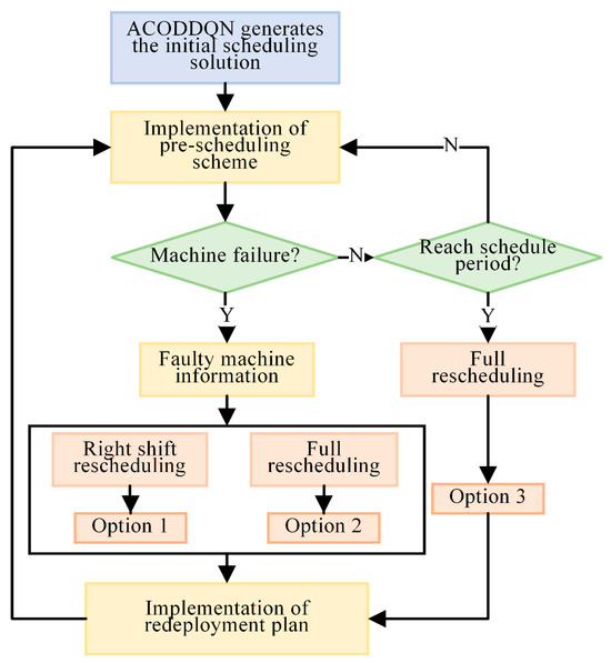
Figure 1. Rescheduling strategy.

3. ACODDQN for MMO-DFJSP

The dynamic scheduling of flexible job shops is an NP-hard problem, and the Ant Colony Optimization (ACO) Algorithm [35,36] has been widely used to solve this problem. However, ACO has slow convergence and poor robustness in large-scale and dynamic environments. Deep reinforcement learning (DRL), especially the double-depth Q-network, DDQN [37,38], has demonstrated its potential to deal with complex scheduling problems by learning the optimal policy through interacting with the environment. However, it still faces the problem of slow convergence speed. To cope with these challenges, this paper proposes a self-learning Ant Colony Algorithm (ACODDQN) that combines ACO and DDQN, which integrates the advantages of global search and local optimization to solve complex scheduling problems more efficiently.

3.1. ACO Algorithm

The Ant Colony Optimization (ACO) Algorithm is a colony intelligence bionic algorithm derived from the process of simulating the foraging behavior of ants. In solving the dynamic flexible job shop scheduling problem (DFJSP), ACO explores the scheduling solution space by mimicking the behavior of ants looking for food. Each ant selects the machine and execution order of each process in the solution space, thus forming a complete scheduling solution. The core idea of ACO is to guide the search process through pheromone updating and collaboration among ants to gradually approach the global optimal solution. The specific algorithm flow is shown in Figure 2.

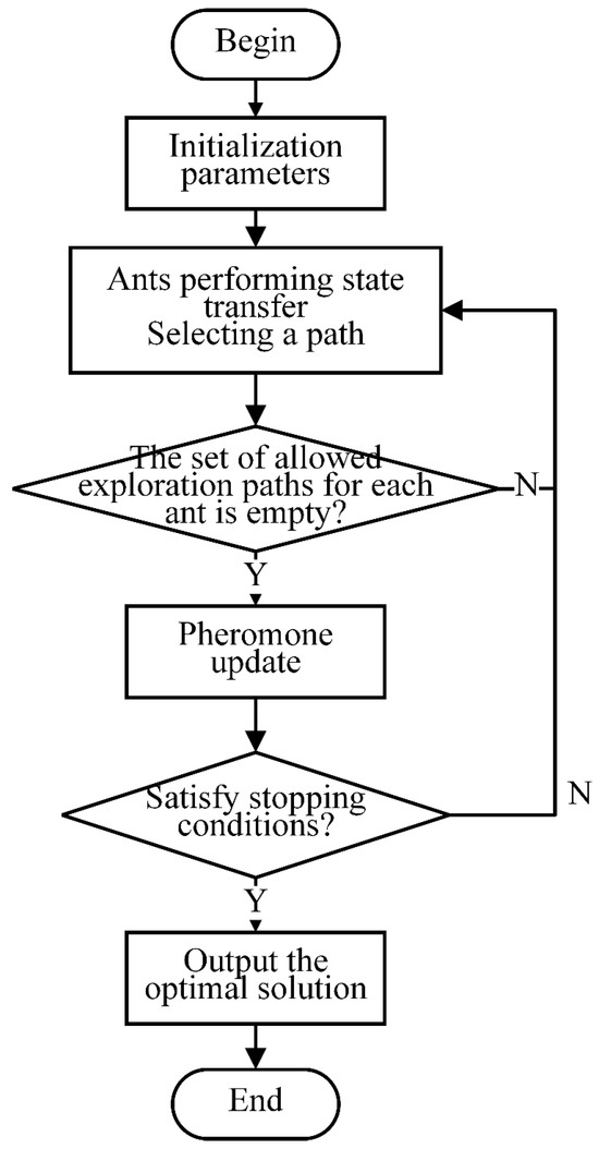
Figure 2. Flowchart of the ACO Algorithm.

3.2. DDQN Algorithm

The DDQN algorithm is a deep reinforcement learning algorithm based on value functions, which aims to solve the high estimation problem in the traditional DQN algorithm. By introducing the goal network mechanism, the DDQN algorithm first evaluates the advantages and disadvantages of action selection, selects them, and then uses the goal network to estimate the goal Q-value. This approach effectively avoids overestimation in solving the multi-objective flexible job shop scheduling problem by decoupling the computation of action selection and target Q-value, thus reducing model bias.

When solving the large-scale multi-objective flexible job shop scheduling problem, the DDQN algorithm optimizes the scheduling strategy by continuously learning the intelligence. Its pseudo-code, shown in Algorithm 1, describes the key steps and update rules throughout the algorithm.

Algorithm 1. DDQN Algorithm
Input: D-empty reply: $\theta$-initial network parameters;${\theta }^{\prime }$ copy of $\theta$; Nb-training batch size; Nr-reply buffer maximum size; $N^{\prime }$-target network replacement freq. Output: Parameters of network
1:	for episode e ∈ {1,2,…,M}, do
2:	Initializing frame sequence x ←()
3:	for t ∈ {0,1,…}, do
4:	Set state s←x, sample action a~${\pi }_b$
5:	Sample next frame $x^t$ from environment $\epsilon$ given (s,a), receive reward r, append $x^t$ to x
6:	if |x| > Nf, then delete oldest frame $x_{tmin}$ from x end
7:	Set s’←x, add transition tuple (s,a,r,s’) to d
8:	Replace the oldest tuple if |D| ≥ Nr
9:	Sample a min-batch of Nb tuples (s,a,r,s’) to Unif (D)
10:	Construct target values, one for each of the Nb tuples
11:	Define amax(s’,$\theta$) = argmaxa. Q (s’; a’; $\theta$)
12:	$y_r=\left\{\begin{array}{c} r , if s is terminal\\ r+\gamma Q(s’, a^{max }(s’;\theta );\theta ’), otherwise\end{array}\right.$
13:	Do gradient decent step with loss ${\left|\right|{\gamma }_i-Q(s,a;\theta )\left|\right| }^2$
14:	Replace target parameters ${\theta }^{\prime }$←$\theta$ every N’ steps
15:	end
16:	end

3.3. ACODDQN Algorithm

The core idea of the ACODDQN algorithm is to combine the Ant Colony Optimization (ACO) Algorithm with the double-depth Q-network (DDQN), which performs an iterative search in the solution space through the pheromone-guided and updating mechanism and gradually approaches the optimal scheduling scheme. Meanwhile, the DDQN algorithm optimizes the parameters in the ACO through reinforcement learning to cope with the dynamic changes and challenges in the complex flexible job shop scheduling problem.

3.3.1. ACODDQN Algorithm Framework

The ACODDQN algorithm framework is shown in Figure 3. The steps of the ACODDQN algorithm are detailed below:

Step 1: Initialize algorithm parameters. To provide the base settings for algorithm execution, initialize the pheromone matrix in the ACO Algorithm and the DDQN parameters.

Step 2: The ant colony searches the solution space. The Ant Colony Algorithm explores the solution space, selects the next visited node by transferring the probability, constructs the path, and keeps searching until it traverses all the nodes and records the ants’ exploration path.

Step 3: State space construction. Record the feasible solution for the ant exploration path in the state space of the DDQN algorithm.

Step 4: Pheromone update with non-dominated sorting. Rank the solutions by non-dominated sorting and assign different ranks to update the pheromone, strengthen the selection of high-quality solutions, and optimize the pheromone guidance.

Step 5: Iteration with DDQN training. Determine whether the preset number of iterations has been reached. If not, use DDQN to train the ant colony path and select N feasible solutions to continue the search.

Step 6: Feasible solution division. Assign valid feasible solutions based on uniform weights to ensure the diversity of the solution set.

Step 7: Monte Carlo feasibility validation. Verify the feasibility of the solutions using Monte Carlo simulation methods to ensure that they satisfy the scheduling constraints.

Step 8: Output Pareto optimal solution set. Output a valid Pareto optimal solution set that provides a balanced solution to the multi-objective scheduling problem.

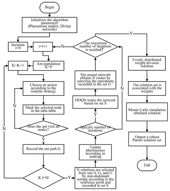
Figure 3. Flowchart of the ACODDQN algorithm.

3.3.2. Ant Colony Search Solution Space

In the ACODDQN algorithm, ants explore the solution space by simulating natural foraging behavior. The process can be described as follows:

(1) Initialization: Set the initial number of ants to 0 and gradually increase it. Each ant represents a solution explorer and adopts a roulette selection strategy to choose the next node among the unvisited nodes. The probability of selection is jointly determined by pheromone concentration and heuristic information;

(2) Node selection and taboo table update: The ants perform node selection based on the roulette selection strategy and add the visited nodes to the taboo table to avoid repeated visits. The taboo table is updated instantly after each node selection to ensure the diversity of path exploration;

(3) Path completion and recording: The ants select nodes until all nodes are visited and path exploration is completed. After path completion, path G and its quality metrics (e.g., path length or objective value) are recorded, and the path is used as part of the current solution to provide a reference for subsequent optimization and decision-making.

3.3.3. Non-Dominant Sort

In the previous section, the use of an ant colony to explore the solution space has been proposed. Next, non-dominated ordering will be used to evaluate the merits of the generated solutions, so as to ensure that the solution set can effectively cover the Pareto front, which is designed as follows:

(1) Solution set generation: Each time, a set of solutions is generated through an ant exploration process, each generated by ants under a roulette selection strategy. Specifically, the ants choose the decisions of artifact scheduling (artifact $i$ is assigned to machine $k$), machine assignment (machine $k$ is used in the order), and repairer scheduling (repairer $w$ repairs machine $k$). Each solution corresponds to a specific scheduling scheme involving the start and end times of tasks and the assignment of repair tasks.

(2) Dominance relations and ordering: The dominance relations between each pair of solutions are computed, and a non-dominated ordering of the solution set is performed to classify the solution set into multiple classes. The solutions in the solution set are ranked based on the Pareto front and their congestion is evaluated, which is mainly ranked for each objective, and the distance d between the solution and the neighboring solutions is calculated as follows:

$$Crowding degree\left(Q\right)={\displaystyle \sum }_i{\displaystyle \frac{d_i}{d_{max}}}$$

(16)

where $d_i$ is the distance on target $i$ and $d_{max}$ is the maximum distance on that target dimension.

(3) Selection of optimal solution: The optimal solution is selected based on the non-dominated ranking and the degree of congestion. To ensure the quality and diversity of solutions, preference is given to solutions with a low dominance rank (closer to the Pareto front) and higher congestion.

3.3.4. Pheromone Update Mechanism

In the ACODDQN algorithm, the definition of state space and action space provides the basis for learning and decision-making for intelligence. However, the pheromone update mechanism becomes crucial in optimizing the scheduling strategy further and improving the algorithm’s search efficiency and convergence speed. The pheromone is not only related to the quality of path selection, but also needs to be updated with the Q-value in the DDQN algorithm to achieve an effective combination of ACO and DDQN. This mechanism is designed to enhance the role of pheromones in guiding the DDQN learning process and optimize the overall search strategy.

First, to adapt the pheromone update to the dynamic search progress of the algorithm, we designed the adaptive evaporation rate mechanism. This mechanism dynamically adjusts the evaporation rate according to the algorithm’s current search progress to make the pheromone evaporation more reasonable. Its calculation formula is as follows:

$$p\left(t\right)=p_0\times \left(1-{\displaystyle \frac{t}{T_{\max }}}\right)$$

(17)

$P_0$ is the initial evaporation rate; $T_{\max }$ is the maximum number of iterations; and $t$ is the current number of iterations.

Next, we design the adaptive pheromone increment mechanism to better guide the ants in selecting quality paths. This mechanism adjusts the pheromone increment through the Q-value learning progress in the DDQN algorithm to improve the quality of path selection. Its increment calculation formula is as follows:

$$\Delta {\tau }_{ij}(t)={\displaystyle \frac{Q}{L_{ij}}}\times \left(1+a\times Q\left(s,a\right)\right)$$

(18)

$Q\left(s,a\right)$ is the Q-value of the DDQN as state s and action a; $a$ is a constant, used to adjust the degree of influence of the Q-value on pheromone increment; and $L_{ij}$ is the path mass.

In order to further enhance the pheromone guidance, the mechanism of forward and reverse pheromone updating was adopted. During forward updating, ants tend to choose the path with a higher pheromone concentration. After each Q-value update, the pheromone will be adjusted in the reverse direction according to the change in the Q-value. Its updating formula is as follows:

$${\tau }_{ij}(t+1)=(1-p\left(t\right))\times t_{ij}\left(t\right)+\Delta {\tau }_{ij}\left(t\right)\times (1+\beta \times \Delta Q\left(s,a\right))$$

(19)

$\Delta Q\left(s,a\right)$ is the change in the Q-value of state s and action a in DDQN and $\beta$ is a constant used to regulate the effect of changes in the Q-value on pheromone renewal.

In summary, the final pheromone update mechanism can be expressed as follows:

$${\tau }_{ij}(t+1)=(1-p\left(t\right))\times t_{ij}(t)+{\displaystyle \frac{Q}{L_{ij}}}\times \left(1+a\times Q\left(s,a\right)\right)\times (1+\beta \times \Delta Q\left(s,a\right))$$

(20)

Through the above design, the pheromone updating mechanism can dynamically reflect the superior and inferior paths in the search process and simultaneously combine with the feedback mechanism of the Q-value to further optimize the search strategy and accelerate convergence.

3.3.5. DDQN Framework

To further optimize the scheduling strategy, the DDQN algorithmic framework is designed in this section to enhance the learning capability and improve the optimization of the solutions generated by the ACO Algorithm.

(1)

State set

In the solution space exploration phase of the ACO Algorithm (Section 3.3.2), the ants generate the initial scheduling solution through a roulette wheel selection strategy. To ensure the effectiveness of subsequent optimization, the ACODDQN framework introduces a state space design. The quality of scheduling decisions relies on accurately perceiving the current production state. By computing real-time shop floor processing information, we construct state feature vectors reflecting the production environment to minimize the delay and completion times. The state features include the average completion time, the standard deviation of completion time, the average delay time, and the standard deviation of delay time of the workpiece.

$$C_{ave}={\displaystyle \frac{{{\displaystyle \sum }}_{i=1}^N{C}_i}{N}}$$

(21)

$$C_{std}=\sqrt{{\displaystyle \frac{{{\displaystyle \sum }}_{i=1}^N{\left(C_i-C_{ave}\right)}^2}{N}}}$$

(22)

$${DT}_{ave}={\displaystyle \frac{{{\displaystyle \sum }}_{i=1}^N{DT}_i}{N}}$$

(23)

$${DT}_{std}=\sqrt{{\displaystyle \frac{{{\displaystyle \sum }}_{i=1}^N{\left({DT}_i-{DT}_{ave}\right)}^2}{N}}}$$

(24)

Equations (21)–(24) represent the four state characteristics. Equation (21) represents the average completion time of all artifacts and Equation (22) represents the standard deviation of the completion time of all artifacts. Equation (23) represents the average delay time of all artifacts and Equation (24) represents the standard deviation of the delay time of all artifacts.

(2)

Action state

In the aforementioned non-dominated sorting (Section 3.3.3), we ensured the distribution of different solutions in the Pareto front by sorting the generated solution set. In order to cope with complex production environments, the DDQN framework needs to optimize the action selection further for the initial solutions generated by the ACO Algorithm. To this end, we designed composite scheduling rules in the DDQN framework for the selection of workpieces, machines, and maintenance workers, respectively: one, two, and two scheduling rules for workpieces, machines, and maintenance workers, and four composite scheduling rules are formed by different combinations, as shown in Table 3, aiming to optimize the dynamic scheduling and co-scheduling of the maintenance workers for machine failures.

Table 3. Combined strategies of four composite scheduling rules.

Composite Scheduling Rule	Job Scheduling Rule	Machine Scheduling Rule	Maintenance Worker Scheduling Rule
Rule1	J1	M1	W1
Rule2	J1	M2	W1
Rule3	J1	M1	W2
Rule4	J1	M2	W2

The workpiece scheduling rule J1 follows the first-in-first-out (FIFO) principle.

Machine scheduling rule M1 selects the earliest available machine and M2 selects the machine with the longest idle time.

Maintenance worker scheduling rule W1 selects the maintenance worker with the longest idle time and W2 selects the available worker with the shortest maintenance time.

(3)

Reward

In the pheromone update mechanism (Section 3.3.4), the concentration of pheromones reflects the quality of the current solution and guides the generation of subsequent solutions. In the DDQN framework, the reward function is designed to enhance the scheduling optimization further. In order to solve the multi-objective optimization problem (minimizing the delay time and completion time), this paper proposes a systematic reward function design scheme combining a weighted reward function, multi-objective optimization, and a penalty mechanism, aiming to balance the optimization effects of different objectives and ensure the feasibility and efficiency of the solution.

Firstly, in order to balance the two objectives of delay time $DT\left(s,a\right)$ and completion time $C_{\max }\left(s,a\right)$ in the optimization process, this paper uses the weighted sum method to design the reward function in the following form:

$$R^{*}\left(s,a\right)=w_1\times DT\left(s,a\right)+w_2\times C_{\max }\left(s,a\right)$$

(25)

where $w_1$ and $w_2$ are the weighting coefficients of delay time and completion time, respectively, and satisfying $w_1$ + $w_2$ = 1 ensures a balanced contribution of the two objectives in the optimization process.

In order to avoid the impact of imbalance between the objectives due to different magnitudes, the delay time and completion time are normalized in this paper and mapped to a uniform range of values. The normalized reward function is of the following forms:

$$D{T}^{\prime }\left(s,a\right)={\displaystyle \frac{DT}{\max \left(DT\right)}}$$

(26)

$${C^{\prime }}_{\max }\left(s,a\right)={\displaystyle \frac{C_{\max }}{\max \left(C_{\max }\right)}}$$

(27)

$$R^{\prime }\left(s,a\right)=w_1\times D{T}^{\prime }\left(s,a\right)+w_2\times {C^{\prime }}_{\max }\left(s,a\right)$$

(28)

In order to ensure the feasibility of the solution process and to avoid the generation of invalid solutions, a penalty mechanism is designed in this paper. If the scheduling scheme increases the delay or completion time, the penalty mechanism guides the model away from non-compliant solutions through negative rewards. The following formula calculates the penalty term:

$$R_{penalty}\left(s,a\right)=-\alpha \times (D{T}^{\prime }\left(s,a\right)+{C^{\prime }}_{\max }\left(s,a\right))$$

(29)

where $\alpha$ is a penalty coefficient that adjusts the strength of the negative reward to ensure that the model avoids ineffective or inefficient scheduling schemes.

Combining the above designs, the final reward function takes the following form:

$$R\left(s,a\right)=w_1\times D{T}^{\prime }\left(s,a\right)+w_2\times {C^{\prime }}_{\max }\left(s,a\right)+R_{penalty}\left(s,a\right)$$

(30)

This function can balance the two objectives of delay time and completion time in the optimization process and, at the same time, improve the quality of the scheduling solution by constraining the solutions that do not meet the constraints through a penalty mechanism.

3.3.6. Feasible Solution Optimization

In the ACODDQN algorithm, a diversity partition mechanism of uniform weight distribution is adopted to ensure the diversity of the solution set and avoid local optimization. First, the feasible solutions are divided into subsets based on uniform weight allocation to ensure that the solution set is evenly distributed in the target space (such as delay and completion time). By calculating the crowding degree, the solution with a high crowding degree is preferentially retained to avoid local clustering. The dynamic weight adjustment formula is as follows:

$$w_{new}=w_{old}+\alpha \times \left(d_{target}-d_{current}\right)$$

(31)

where $d_{target}$ is the density of the target distribution, $d_{current}$ is the density of the current solution set, and $\alpha$ is the adjustment coefficient.

Finally, through the elite retention mechanism combined with non-dominated sorting, the top N high-quality solutions are retained to enter the next iteration to ensure the quality and diversity of the solution set. This mechanism effectively improves the algorithm’s global search ability.

3.3.7. Pareto Optimal Solution Set Generation and Output

In the ACODDQN algorithm, the solution of level 1 is extracted by non-dominant sorting, and the redundant solution is eliminated by combining the crowding sorting to ensure the universality and uniform distribution of the Pareto frontier. The Pareto optimal solution set is stored in a tree structure, where the key is the target vector (e.g., delay time, completion time), and the value is the corresponding scheduling scheme. Through this process, ACODDQN effectively outputs a set of Pareto optimal solutions that meet the needs of multi-objective optimization.

4. Experiment and Discussion

4.1. Extension Examples

The simulation experiment is implemented in the Matlab (Matlab2020a) language environment. Due to the lack of a general benchmark considering maintenance personnel resources in DFJSP problems, to verify the performance of the ACODDQN algorithm, this study conducted a test by extending the existing MK01-15 [39] benchmark example. The proposed model combined dynamic production scheduling with maintenance personnel’s maintenance of faulty machines. The added machine failure and maintenance personnel-related parameters for the MK01-15 test set are as follows:

(1) It is known that there are $k$ machines, $w$ maintenance personnel, and a production cycle $C$. For each machine $k$, determine its downtime;

(2) The maintenance personnel determine the maintenance time, and the maintenance time is $T_{repair}~N\left[{\mu }_w,{\sigma }_w\right]$. If $T_k$≤$T_{current}$, the faulty machine $k$ is determined to be repaired by the maintenance worker $w$, $T_{repair,w,k}~N\left[{\mu }_w,{\sigma }_w\right]$;

(3) The dynamic scheduling of the whole system is carried out via real-time simulation to ensure that the maintenance personnel can deal with machine failure when it occurs and meet the maintenance personnel’s ability and machine’s maintenance requirements.

Considering the above factors, the extended example is MWK01-15, in which the processing time, maintenance time, and workpiece urgency fluctuate within a specific range. The extended example is shown in Table 4.

Table 4. Parameters of numerical instances.

Instance	${\mathit{t}}_{\mathit{w}}^{\mathit{k}}$	${\mathit{n}}_{\mathit{i}}$	$\mathit{m}$	$\mathit{q}$	${\mathit{t}}_{\mathit{ij}}$	${\mathit{t}}_{\mathit{w}}^{\mathit{k}}$	$\mathit{U}{\mathit{P}}_{\mathit{i}}$
MWK01	10	6	10	3	[1, 25]	[1, 18]	[1, 3]
MWK02	10	6	10	5	[1, 25]	[1, 18]	[1, 3]
MWK03	15	9	8	3	[1, 19]	[1, 20]	[1, 3]
MWK04	15	14	15	5	[1, 35]	[1, 20]	[1, 3]
MWK05	15	15	10	5	[4, 29]	[1, 24]	[1, 3]
MWK06	15	9	4	3	[1, 19]	[2, 24]	[1, 3]
MWK07	20	5	10	3	[1, 21]	[2, 29]	[1, 3]
MWK08	20	7	10	5	[1, 21]	[1, 31]	[1, 3]
MWK09	20	9	15	3	[4, 27]	[1, 27]	[1, 3]
MWK10	20	12	15	5	[5, 39]	[4, 30]	[1, 3]
MWK11	30	9	6	3	[10, 29]	[2, 28]	[1, 3]
MWK12	30	7	10	5	[10, 29]	[2, 28]	[1, 3]
MWK13	30	15	15	5	[10, 29]	[1, 27]	[1, 3]
MWK14	30	9	15	5	[10, 29]	[1, 24]	[1, 3]
MWK15	30	11	25	5	[10, 29]	[3, 16]	[1, 3]

4.2. Parameter Settings

For the ACODDQN algorithm, most of these parameters are random variables that fluctuate within a fixed range, so the optimal values of the parameters need to be determined. In this paper, we use Taguchi experiments to determine the optimal parameter values for the ACODDQN algorithm, which mainly involves the relevant parameters of the ACO and DDQN algorithms, with five levels set for each factor. The parameter design is shown in Table 5.

Table 5. Orthogonal test parameters.

Parameter	Parameter Level
	1	2	3	4	5
$m$	100	125	150	175	200
$\rho$	0.1	0.2	0.3	0.4	0.5
$\alpha$	0.01	0.02	0.03	0.04	0.05
$\gamma$	0.7	0.75	0.8	0.85	0.9
$\epsilon$	0.1	0.2	0.3	0.4	0.5

In Table 4, $m$ represents the ant colony number; $\rho$ is pheromone volatilization rate; $\alpha$ is the learning rate; $\gamma$ is the discount factor; and $\epsilon$ is the greed rate.

The orthogonal test in this paper is based on five levels and five factors, so the L25 (5^5) orthogonal table is chosen. According to the orthogonal test parameter table, MWK10 was selected as the main example of the orthogonal test, and the ACODDQN algorithm changed the relevant parameter values. Each parameter value was run 20 times to obtain 20 different solution sets under this parameter. Then, the 20 solution sets were combined, and their Pareto frontier was determined as the optimal solution under this set of parameters. At the same time, the HV index of the solution set is selected as the comprehensive evaluation index of the orthogonal experiment. In order to observe the experimental results more clearly, the HV values of the five levels of the same factor were summed and averaged, defined as the influence factor of the factor on the example. The resulting graph was drawn, as shown in Figure 4. It can be seen from Figure 4 that when the number of ants ($m$ = 175) significantly increased the HV value, it was helpful to explore the solution space fully. A low pheromone volatilization rate ($\rho$ = 0.1) maintains a high HV value and avoids premature convergence. Smaller learning rates ($\alpha$ = 0.03) guarantee stable convergence. The discount factor ($\gamma$ = 0.85) balances short- and long-term goals to improve performance. The low greed ratio ($\epsilon$ = 0.1) ensures that the algorithm is stable and avoids over-reliance on the current optimal solution. The final optimal parameters are as follows: $m$ = 175, $\rho$ = 0.1, $\alpha$ = 0.03, $\gamma$ = 0.85, $\epsilon$ = 0.1.

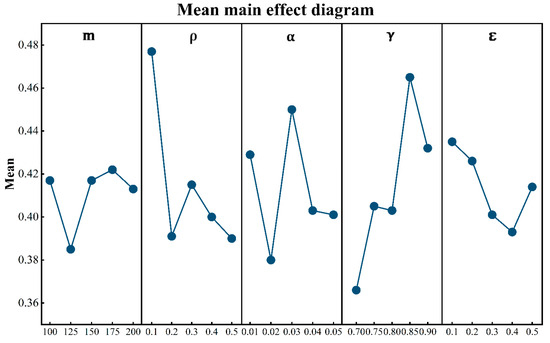
Figure 4. Main parameters SNR line chart.

4.3. Evaluation Indicators

The SP, IGD, and HV [40] indexes comprehensively evaluate the multi-objective solution set’s uniformity, convergence, and diversity.

$$SP(N)=\sqrt{{\displaystyle \frac{{{\displaystyle \sum }}_i^N(\overline{d_i }-d_i{)}^2}{\left|N-1\right|}}}$$

(32)

where $d_i$ is the manhattan distance between two points and $N$ is the population size. The smaller the SP value, the more uniform the distribution of the solutions and the better the diversity of the solutions.

$$IGD(P,P^{*})={\displaystyle \frac{{{\displaystyle \sum }}_{x\in p^{*}}dis(x,P)}{\left|P^{*}\right|}}$$

(33)

where $P$ is the solution set of the ACODDQN algorithm, $P^{*}$ the uniform sampling set of true Pareto fronts, and $dis(x,P)$ the Euclidean distance between $P^{*}$ and $P$. Smaller values of IGD represent the better quality of the solution set composite.

$$HV=\delta \times (U_{i=1}^{\left|S\right|}{V}_i)$$

(34)

where $\delta$ denotes the Lebesgue measure and $\left|S\right|$ is used to measure the volume. denotes the number of non-dominated solution sets, and $V_i$ denotes the hypervolume formed by the reference point and the ith solution in the solution set. Larger values of HV indicate the better homogeneity and diversity of the algorithm’s results.

4.4. The Experimental Results of the Extended Example

4.4.1. Comparison with the Composite Scheduling Rule

This paper compares the ACODDQN algorithm with four compound scheduling rules in detail. The optimal results are marked in bold through 20 independent runs of 15 extended examples and the average processing of each evaluation index, and relevant statistical results are obtained (Table 6). As seen from Table 6, compared with the composite scheduling rule, the ACODDQN algorithm performs best in SP, IGD, and HV. In these three indexes, the ACODDQN algorithm (93.3%, 93.3%, and 100%) is superior to the other four compound scheduling rules, which proves that the ACODDQN algorithm has apparent advantages in convergence, uniformity, and diversity compared with other scheduling rules. The average time of 20 runs of the ACODDQN algorithm and four composite scheduling rules in 15 extended calculation examples is shown in Table 7, and the shortest time is marked in bold. It can be seen from Table 7 that the ACODDQN algorithm shows the shortest running time in the calculation examples of different scales. This shows that the ACODDQN algorithm has substantial solution accuracy and a significant advantage in computing efficiency.

Table 6. Comparative analysis of average SP, IGD, and HV scores for ACODDQN and composite scheduling rules.

Instance	SP					IGD					HV
	ACO DDQN	Rule1	Rule2	Rule3	Rule4	ACO DDQN	Rule1	Rule2	Rule3	Rule4	ACO DDQN	Rule1	Rule2	Rule3	Rule4
MWK 01	0.001	0.156	0.244	0.223	0.278	0.001	0.173	0.283	0.2492	0.249	0.317	0.127	0.073	0.098	0.012
MWK 02	0.006	0.178	0.307	0.299	0.418	0.008	0.214	0.318	0.324	0.415	0.412	0.221	0.084	0.178	0.061
MWK 03	0.018	0.217	0.317	0.264	0.348	0.015	0.231	0.321	0.279	0.377	0.426	0.201	0.101	0.165	0.081
MWK 04	0.087	0.124	0.245	0.199	0.268	0.111	0.278	0.387	0.294	0.476	0.578	0.312	0.088	0.211	0.045
MWK 05	0.017	0.188	0.276	0.264	0.412	0.027	0.215	0.298	0.278	0.465	0.319	0.117	0.064	0.071	0.012
MWK 06	0.168	0.248	0.324	0.345	0.398	0.174	0.141	0.364	0.304	0.534	0.468	0.121	0.041	0.072	0.019
MWK 07	0.075	0.126	0.208	0.167	0.345	0.108	0.147	0.212	0.188	0.378	0.371	0.146	0.073	0.119	0.038
MWK 08	0.001	0.148	0.274	0.211	0.442	0.003	0.167	0.289	0.241	0.454	0.314	0.146	0.069	0.112	0.013
MWK 09	0.078	0.124	0.278	0.225	0.354	0.115	0.197	0.307	0.259	0.394	0.617	0.412	0.217	0.316	0.110
MWK 10	0.001	0.124	0.279	0.188	0.317	0.001	0.121	0.297	0.226	0.324	0.407	0.201	0.062	0.123	0.032
MWK 11	0.112	0.176	0.236	0.185	0.318	0.128	0.189	0.243	0.198	0.337	0.509	0.347	0.124	0.173	0.081
MWK 12	0.112	0.098	0.247	0.164	0.324	0.117	0.197	0.378	0.241	0.489	0.462	0.217	0.114	0.162	0.046
MWK 13	0.224	0.288	0.398	0.327	0.412	0.245	0.317	0.408	0.387	0.489	0.586	0.317	0.114	0.265	0.072
MWK 14	0.115	0.228	0.364	0.308	0.378	0.167	0.291	0.378	0.322	0.408	0.496	0.328	0.102	0.267	0.041
MWK 15	0.116	0.317	0.402	0.379	0.409	0.218	0.347	0.466	0.461	0.507	0.617	0.318	0.106	0.217	0.071

Table 7. Average running time of ACODDQN algorithm and four compound scheduling rules.

T/s	Instance	MWK01	MWK02	MWK03	MWK04	MWK05	MWK06	MWK07	MWK08	MWK09	MWK10	MWK11	MWK12	MWK13	MWK14	MWK15
	ACO DDQN	52	55	68	63	67	73	81	59	76	68	72	75	86	89	95
	Rule1	62	69	77	98	107	112	134	176	136	116	136	199	279	185	221
	Rule2	72	85	103	136	175	178	196	335	229	207	346	319	514	346	389
	Rule3	69	77	79	104	120	157	180	246	161	176	196	208	364	264	251
	Rule4	89	109	145	180	214	267	349	368	346	380	426	657	616	765	796

4.4.2. Comparing Algorithms

In order to verify the performance of the proposed ACODDQN algorithm for solving the MMO-DFJSP model, 15 extended examples were used to compare the ACODDQN algorithm with MOPSO [41], IGWO [42], NSGA-II [43], DDQN [44], PPO [45], and GA [46]. The optimal results are marked in bold through 20 independent runs of 15 extended examples and the average processing of each evaluation index, and relevant statistical results are obtained (Table 8 and Table 9). As can be seen from Table 8, in both the SP and IGD indexes, the ACODDQN algorithm outperformed the other six algorithms in thirteen experiments (86.7%). As can be seen from Table 9, among the HV indicators, the ACODDQN algorithm outperformed the other six algorithms in thirteen experiments (93%), indicating that the ACODDQN algorithm has obvious advantages in terms of convergence, diversity, and coverage. In order to more intuitively show the average performance of the SP, IGD, and HV indicators of each algorithm in solving extended examples, the indicators of three extended examples, MWK02, MWK05, and MWK10, are drawn as box diagrams (Figure 5). As can be seen from Figure 5, compared with the other six algorithms, the ACODDQN algorithm has the lowest mean value of the SP and IGD indicators and the highest mean value of the HV indicators, and the index range fluctuated less, indicating that ACODDQN is superior to other algorithms in terms of solution quality and stability. In addition, the average time of twenty runs between the ACODDQN algorithm and six comparison algorithms in fifteen extended examples was counted, and the shortest time was marked in bold, as shown in Table 10. It can be seen from Table 10 that with the expansion of the scale of extended examples, the running time gap between the ACODDQN algorithm and the other six comparison algorithms gradually increased. Moreover, the ACODDQN algorithm always shows the shortest running time in all the extended examples, which fully proves the excellent solving efficiency of the ACODDQN algorithm.

Table 8. Comparison of average SP and IGD scores between ACODDQN and six algorithms.

Instance	SP							IGD
	ACO DDQN	IGWO	NSGA II	PPO	MO PSO	DDQN	GA	ACO DDQN	IGWO	NSGA II	PPO	MO PSO	DDQN	GA
MWK01	0.065	0.131	0.211	0.074	0.251	0.083	0.327	0.018	0.226	0.266	0.185	0.325	0.203	0.350
MWK02	0.050	0.335	0.431	0.332	0.497	0.347	0.525	0.239	0.408	0.430	0.393	0.384	0.396	0.411
MWK03	0.059	0.181	0.225	0.051	0.371	0.102	0.245	0.111	0.263	0.292	0.152	0.329	0.196	0.367
MWK04	0.036	0.211	0.294	0.047	0.336	0.119	0.406	0.198	0.386	0.456	0.124	0.561	0.213	0.536
MWK05	0.024	0.220	0.388	0.164	0.447	0.229	0.438	0.195	0.345	0.472	0.247	0.497	0.346	0.521
MWK06	0.049	0.147	0.199	0.025	0.281	0.088	0.334	0.146	0.257	0.280	0.197	0.313	0.213	0.282
MWK07	0.041	0.154	0.253	0.072	0.331	0.102	0.293	0.134	0.212	0.273	0.177	0.395	0.193	0.369
MWK08	0.080	0.362	0.476	0.198	0.532	0.299	0.554	0.156	0.446	0.501	0.202	0.540	0.340	0.465
MWK09	0.090	0.176	0.292	0.104	0.334	0.133	0.345	0.189	0.454	0.521	0.192	0.589	0.221	0.581
MWK10	0.176	0.355	0.471	0.279	0.517	0.351	0.504	0.288	0.438	0.473	0.344	0.502	0.367	0.393
MWK11	0.237	0.567	0.669	0.315	0.712	0.472	0.694	0.399	0.578	0.672	0.347	0.734	0.486	0.674
MWK12	0.109	0.324	0.377	0.269	0.407	0.312	0.427	0.156	0.356	0.398	0.277	0.426	0.341	0.455
MWK13	0.205	0.331	0.341	0.247	0.411	0.267	0.431	0.232	0.342	0.359	0.261	0.435	0.279	0.410
MWK14	0.167	0.378	0.381	0.222	0.415	0.271	0.365	0.188	0.394	0.416	0.264	0.507	0.289	0.448
MWK15	0.116	0.345	0.388	0.269	0.416	0.305	0.430	0.136	0.367	0.411	0.297	0.465	0.324	0.402

Table 9. Comparison of average HV scores between ACODDQN and six algorithms.

Instance		MWK01	MWK02	MWK03	MWK04	MWK05	MWK06	MWK07	MWK08	MWK09	MWK10	MWK11	MWK12	MWK13	MWK14	MWK15
HV	ACO DDQN	0.611	0.347	0.371	0.624	0.581	0.390	0.281	0.513	0.327	0.142	0.417	0.191	0.137	0.288	0.131
	IGWO	0.234	0.013	0.191	0.012	0.214	0.017	0.098	0.311	0.059	0.038	0.119	0.046	0.076	0.124	0.056
	NSGAII	0.107	0.004	0.051	0.01	0.205	0.012	0.083	0.137	0.035	0.023	0.084	0.008	0.036	0.107	0.035
	PPO	0.552	0.135	0.262	0.261	0.476	0.390	0.136	0.528	0.182	0.117	0.323	0.129	0.124	0.214	0.112
	MOPSO	0.004	0.006	0.032	0.004	0.365	0.012	0.081	0.134	0.027	0.017	0.042	0.005	0.026	0.082	0.032
	DDQN	0.495	0.111	0.214	0.207	0.101	0.312	0.123	0.352	0.192	0.054	0.317	0.092	0.101	0.195	0.081
	GA	0.003	0.001	0.018	0.006	0.093	0.002	0.095	0.115	0.030	0.029	0.044	0.025	0.021	0.131	0.035

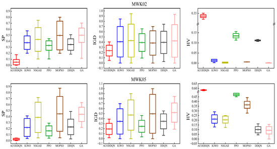
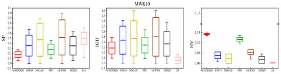
Figure 5. Boxplots of average SP, IGD, and HV metrics for MWK02, MWK05, and MWK10 instances.

Table 10. Average running time of ACODDQN and six algorithms.

Instance		MWK01	MWK02	MWK03	MWK04	MWK05	MWK06	MWK07	MWK08	MWK09	MWK10	MWK11	MWK12	MWK13	MWK14	MWK15
T/s	ACO DDQN	52	55	68	63	67	73	81	59	76	68	72	75	86	89	95
	IGWO	56	57	94	72	88	147	153	68	162	105	160	163	162	161	188
	NSGA II	73	76	108	96	100	172	200	91	212	124	196	206	212	193	228
	PPO	81	104	162	136	142	236	241	124	294	180	246	270	294	239	305
	MOPSO	96	82	121	109	110	210	159	99	164	132	189	178	164	168	197
	DDQN	102	105	122	121	117	227	235	130	265	129	214	239	265	205	265
	GA	152	166	183	172	160	246	267	143	302	135	236	251	301	246	368

In order to further analyze the performance advantages of the ACODDQN algorithm in solving dynamic scheduling problems, four extended examples of MWK01, MWK02, MWK04, and MWK10 were selected in this paper, and the key parameters ($m$, $i$, $w$, and ${UP}_i$) in each example are shown. The ACODDQN algorithm and six other algorithms were used to run these four extended examples twenty times independently, average the target values of the twenty times, and finally draw the results, as shown in Figure 6. As seen from Figure 6, among the four extended examples shown, the ACODDQN algorithm shows significant advantages for the two optimization objectives of minimizing delay time and completion time, which makes it superior compared to other comparison algorithms. This result proves that the ACODDQN algorithm can effectively reduce the delay time in production scheduling and significantly shorten overall completion time. Thus, the system’s overall scheduling efficiency can be improved.

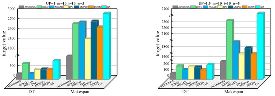
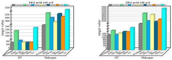
Figure 6. Comparison of average objective values for ACODDQN and six algorithms across MWK01, MWK02, MWK04, and MWK10 instances.

4.5. Case Experiments

4.5.1. Case Description

In order to verify the effectiveness of the ACODDQN algorithm in solving multi-objective dynamic scheduling problems, this study selected a manufacturing flexible processing plant as an example. In the production process of this workshop, machine failure will affect the overall scheduling. Figure 7 shows the plant’s assembly process flow chart. According to the flow, this paper simplifies the workpiece processing information to a 10 × 6 flexible job scheduling problem, as shown in Table 11. Table 12 provides the maintenance time information for machines that can be serviced by maintenance personnel. A 10 × 6 × 3 multi-objective flexible job shop scheduling problem is formed by incorporating maintenance personnel scheduling into a flexible job shop scheduling problem. This example further verifies the effectiveness and advantages of the ACODDQN algorithm in solving dynamic scheduling problems.

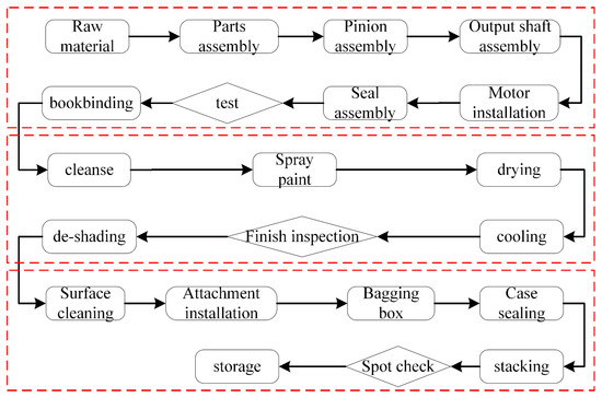
Figure 7. Assembly and processing flowchart.

Table 11. Processing machine information.

Ji	Oij	m1	m2	m3	m4	m5	m6	Ji	Oij	m1	m2	m3	m4	m5	m6
J1	O11	-	-	-	22	16	-	J6	O61		27	16		15
	O12	12	-	21	29	16	-		O62		13	25	28		26
	O13	19	21	-	28	18	-		O63	26	26		27	20	13
	O14	17	-	-	-	23	17	J7	O71	-	20	22	17	-	18
J2	O21	21	28	-	-	19	16		O72	15		19		28
	O22	-	15	21		20	-		O73		14		24	16	27
	O23	25	19	18	53	-	26	J8	O81	28	25		21		20
J3	O31	24		20	22	22	25		O82		19	28		19
	O32			21		23	23		O83	20			22		18
	O33	23	17		19			J9	O91		17	25	24		29
	O34		32	28		29	21		O92	20		21	25	22
J4	O41			18	16	21			O93		18		16		18
	O42		21		24	26	17		O94	21		25		29	23
	O43		27		18	20	22	J10	O101		20		18	24
J5	O51	23	24	17		21	17		O10.2	15	18	19	18	16	22
	O52	30		12	23	25	26		O10.3	14			12		16
	O53		22		18		19		O10.4		23	24		27
	O54	21	26	23		27			O10.5	22		17	18		19

Table 12. Repairable machine information.

	Mi	m1	m2	m3	m4	m5	m6
Wi
W1			12		18		15
W2		8	13	16		19	24
W3		9	15	12	16	22

4.5.2. Case Solving and Analysis

In this study, by considering the influence of machine fault as a dynamic disturbance factor on the production process, the ACODDQN algorithm and six comparison algorithms are used to solve the production scheduling problem based on the scheduling information of the workpiece, machine tool, and maintenance personnel. The optimization goal is to minimize latency and completion time. In the experiment, the ACODDQN algorithm was optimized for 100 iterations with 6 other comparison algorithms, and its performance was evaluated by drawing the target value change curve of each algorithm in the iteration process (Figure 8). The results show that compared with the other six algorithms, the ACODDQN algorithm not only achieves the optimal initial solution with minimum delay and completion times, but also achieves the optimal solution with the fastest convergence speed, which indicates that ACODDQN has a stronger solving ability and stability when solving complex production scheduling problems.

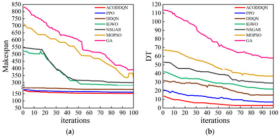
Figure 8. Objective value iteration diagram of the algorithm: (a) Minimize the completion time iteration curve; (b) minimize the delay time iteration curve.

In order to further demonstrate the response effect of the rescheduling mechanism of the ACODDQN algorithm when machine failure occurs, a Gantt diagram of the assembly manufacturing process solved using the ACODDQN algorithm is drawn. The Gantt chart for the initial scheduling shows that the total completion time was 150 min (Figure 9), and that within 60–90 min, machine 2 was temporarily shut down due to a power outage, while machine 3 stopped working due to the wear of mechanical components. Currently, the ACODDQN algorithm’s rescheduling mechanism enables the rescheduling of the processes O10.4 and O2.3 affected by the fault. Specifically, the correct shift scheduling and all rescheduling policies are applied; the unfinished operation O2.3 after the failure of machine 3 is moved right to the available machine 2. In contrast, the unstarted operation O10.4 before the failure of machine 2 is scheduled for the available machine 3. After failure, all processes have been reasonably rescheduled to achieve the minimum completion target. Finally, as shown in Figure 10, the Gantt diagram after the fault repair has a total completion time of 145 min, which is 5 min less than the initial scheduling time, ensuring the regular operation of the factory. At the same time, maintenance workers 1 and 3 are reasonably scheduled to repair machine 2 and machine 3, respectively, and the maintenance arrangement is shown in Figure 11. The results show that although machine fault interrupts production, the production process can be quickly resumed, and the completion time is shorter than the initial scheme thanks to reasonable scheduling and the fault maintenance arrangement of the ACODDQN algorithm, which further verifies the effectiveness and advantages of the ACODDQN algorithm in dynamic scheduling problems.

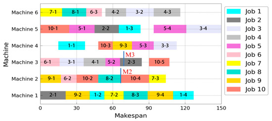
Figure 9. Initial scheduling Gantt chart.

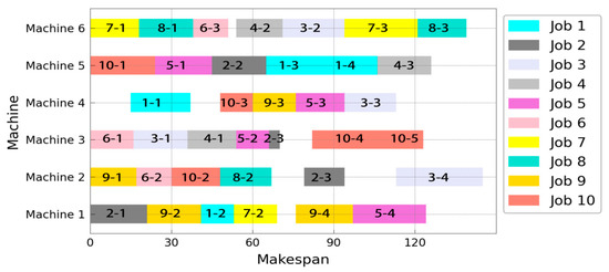
Figure 10. Gantt chart of rescheduling after failure.

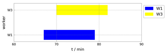
Figure 11. Gantt chart of maintenance worker scheduling.

5. Conclusions

This study proposes a self-learning Ant Colony Algorithm based on deep reinforcement learning (ACODDQN) for the problem of brutal production plan execution due to equipment failure in the dynamic scheduling of a flexible job shop problem (DFJSP). The algorithm integrates the advantages of Ant Colony Optimization (ACO) and the double-depth Q-network (DDQN), explores the solution space through the ACO search mechanism, and combines with non-dominated sorting to screen high-quality solutions to improve the global quality of the solutions and convergence efficiency. Meanwhile, the pheromone updating mechanism dynamically adjusts the search strategy based on the environmental feedback to ensure the adaptability of the optimization direction and avoid the trap of local optimums. The DDQN framework’s introduction further enhances the algorithm’s learning ability, so it has better decision stability and adaptability when coping with stochasticity and unexpected events (e.g., machine failures) in the scheduling environment. In addition, the algorithm locally adjusts the candidate solutions through the feasible solution optimization mechanism to ensure that they satisfy the constraints. It generates the Pareto optimal solution set under the multi-objective optimization framework, which provides high-quality optimization solutions for complex dynamic scheduling problems. The experimental results show that the ACODDQN algorithm exhibits good adaptability and solution performance in minimizing completion and delay times.

This study does not consider the impact of the travel time of maintenance personnel and other potential wastes on the scheduling results, and future studies can take these factors into account to better reflect the actual scheduling scenario.

References

- Niu, H.; Wu, W.; Zhang, T.; Shen, W.; Zhang, T. Adaptive salp swarm algorithm for solving flexible job shop scheduling problem with transportation time. J. Zhejiang Univ. 2023, 57, 1267–1277. [Google Scholar]
- Guo, H.Z.; Wang, Y.T.; Liu, J.J.; Liu, C. Multi-UAV Cooperative Task Offloading and Resource Allocation in 5G Advanced and Beyond. IEEE Trans. Wirel. Commun. 2024, 23, 347–359. [Google Scholar] [CrossRef]
- Tariq, A.; Khan, S.A.; But, W.H.; Javaid, A.; Shehryar, T. An IoT-Enabled Real-Time Dynamic Scheduler for Flexible Job Shop Scheduling (FJSS) in an Industry 4.0-Based Manufacturing Execution System (MES 4.0) (vol 12, pg 49653, 2024). IEEE Access 2024, 12, 118941. [Google Scholar] [CrossRef]
- Wang, J.; Liu, Y.; Ren, S.; Wang, C.; Ma, S. Edge computing-based real-time scheduling for digital twin flexible job shop with variable time window. Robot. Comput.-Integr. Manuf. 2023, 79, 102435. [Google Scholar] [CrossRef]
- Cheng, D.; Lou, S.; Zheng, H.; Hu, B.; Hong, Z.; Feng, Y.; Tan, J. Industrial Exoskeletons for Human-Centric Manufacturing: Challenges, Progress, and Prospects. Comput. Integr. Manuf. Syst. 2024, 30, 4179. [Google Scholar]
- Jiang, Q.; Wei, J. Real-time Scheduling Method for Dynamic Flexible Job Shop Scheduling. J. Syst. Simul. 2024, 36, 1609–1620. [Google Scholar]
- Gen, M.; Lin, L.; Ohwada, H. Advances in Hybrid Evolutionary Algorithms for Fuzzy Flexible Job-shop Scheduling: State-of-the-Art Survey. In Proceedings of the ICAART (1), Online, 4–6 February 2021; pp. 562–573. [Google Scholar]
- Dauzère-Pérès, S.; Ding, J.; Shen, L.; Tamssaouet, K. The flexible job shop scheduling problem: A review. Eur. J. Oper. Res. 2024, 314, 409–432. [Google Scholar] [CrossRef]
- Yue, L.; Peng, K.; Ding, L.S.; Mumtaz, J.; Lin, L.B.; Zou, T. Two-stage double deep Q-network algorithm considering external non-dominant set for multi-objective dynamic flexible job shop scheduling problems. Swarm Evol. Comput. 2024, 90, 13. [Google Scholar] [CrossRef]
- Zhang, G.H.; Lu, X.X.; Liu, X.; Zhang, L.T.; Wei, S.W.; Zhang, W.Q. An effective two-stage algorithm based on convolutional neural network for the bi-objective flexible job shop scheduling problem with machine breakdown. Expert Syst. Appl. 2022, 203, 12. [Google Scholar] [CrossRef]
- Gao, K.; Yang, F.; Li, J.; Sang, H.; Luo, J. Improved jaya algorithm for flexible job shop rescheduling problem. IEEE Access 2020, 8, 86915–86922. [Google Scholar] [CrossRef]
- Luan, F.; Tang, B.; Li, Y.; Liu, S.Q.; Yang, X.; Masoud, M.; Feng, B. Solving multi-objective green flexible job shop scheduling problem by an improved chimp optimization algorithm. J. Intell. Fuzzy Syst. 2024, 46, 7697–7710. [Google Scholar] [CrossRef]
- Lü, Y.; Xu, Z.; Li, C.; Li, L.; Yang, M. Comprehensive Energy Saving Optimization of Processing Parameters and Job Shop Dynamic Scheduling Considering Disturbance Events. J. Mech. Eng. 2022, 58, 242–255. [Google Scholar]
- Yuan, E.D.; Wang, L.J.; Song, S.J.; Cheng, S.L.; Fan, W. Dynamic scheduling for multi-objective flexible job shop via deep reinforcement learning. Appl. Soft Comput. 2025, 171, 13. [Google Scholar] [CrossRef]
- Jimenez, S.H.; Trabelsi, W.; Sauvey, C. Multi-Objective Production Rescheduling: A Systematic Literature Review. Mathematics 2024, 12, 3176. [Google Scholar] [CrossRef]
- Zhang, H.; Xu, J.; Tan, B.; Xu, G. Dual Resource Constrained Flexible Job Shop Energy-saving Scheduling Considering Delivery Time. J. Syst. Simul. 2023, 35, 734–746. [Google Scholar]
- Li, X.; Xing, S. Dynamic scheduling problem of multi-objective dual resource flexible job shop based on improved genetic algorithm. In Proceedings of the 43rd Chinese Control Conference, CCC 2024, Kunming, China, 28–31 July 2024; pp. 2046–2051. [Google Scholar]
- Sun, A.; Song, Y.; Yang, Y.; Lei, Q. Dual Resource-constrained Flexible Job Shop Scheduling Algorithm Considering Machining Quality of Key Jobs. China Mech. Eng. 2022, 33, 2590–2600. [Google Scholar]
- Mokhtari, G.; Abolfathi, M. Dual Resource Constrained Flexible Job-Shop Scheduling with Lexicograph Objectives. J. Ind. Eng. Res. Prod. Syst. 2021, 8, 295–309. [Google Scholar]
- Jiang, B.; Ma, Y.J.; Chen, L.J.; Huang, B.D.; Huang, Y.Y.; Guan, L. A Review on Intelligent Scheduling and Optimization for Flexible Job Shop. Int. J. Control Autom. Syst. 2023, 21, 3127–3150. [Google Scholar] [CrossRef]
- Turkyilmaz, A.; Senvar, O.; Unal, R.; Bulkan, S. A research survey: Heuristic approaches for solving multi objective flexible job shop problems. J. Intell. Manuf. 2020, 31, 1949–1983. [Google Scholar] [CrossRef]
- Long, X.; Zhang, J.; Zhou, K.; Jin, T. Dynamic self-learning artificial bee colony optimization algorithm for flexible job-shop scheduling problem with job insertion. Processes 2022, 10, 571. [Google Scholar] [CrossRef]
- Chen, F.; Xie, W.; Ma, J.; Chen, J.; Wang, X. Textile Flexible Job-Shop Scheduling Based on a Modified Ant Colony Optimization Algorithm. Appl. Sci. 2024, 14, 4082. [Google Scholar] [CrossRef]
- Liang, Z.Y.; Zhong, P.S.; Zhang, C.; Yang, W.L.; Xiong, W.; Yang, S.H.; Meng, J. A genetic algorithm-based approach for flexible job shop rescheduling problem with machine failure interference. Eksploat. I Niezawodn. 2023, 25, 13. [Google Scholar] [CrossRef]
- Chen, Y.; Liao, X.J.; Chen, G.Z.; Hou, Y.J. Dynamic Intelligent Scheduling in Low-Carbon Heterogeneous Distributed Flexible Job Shops with Job Insertions and Transfers. Sensors 2024, 24, 2251. [Google Scholar] [CrossRef]
- Peng, N.; Zheng, Y.; Xiao, Z.; Gong, G.; Huang, D.; Liu, X.; Zhu, K.; Luo, Q. Multi-objective dynamic distributed flexible job shop scheduling problem considering uncertain processing time. Clust. Comput. 2025, 28, 185. [Google Scholar] [CrossRef]
- Su, C.; Zhang, C.; Wang, C.; Cen, W.; Chen, G.; Xie, L. Fast Pareto set approximation for multi-objective flexible job shop scheduling via parallel preference-conditioned graph reinforcement learning. Swarm Evol. Comput. 2024, 88, 101605. [Google Scholar] [CrossRef]
- Liu, C.-L.; Chang, C.-C.; Tseng, C.-J. Actor-critic deep reinforcement learning for solving job shop scheduling problems. IEEE Access 2020, 8, 71752–71762. [Google Scholar] [CrossRef]
- Wang, L.; Hu, X.; Wang, Y.; Xu, S.; Ma, S.; Yang, K.; Liu, Z.; Wang, W. Dynamic job-shop scheduling in smart manufacturing using deep reinforcement learning. Comput. Netw. 2021, 190, 107969. [Google Scholar] [CrossRef]
- Luo, S.; Zhang, L.; Fan, Y. Dynamic multi-objective scheduling for flexible job shop by deep reinforcement learning. Comput. Ind. Eng. 2021, 159, 107489. [Google Scholar] [CrossRef]
- Liu, Y.; Shen, X.; Gu, X.; Peng, T.; Bao, J.; Zhang, D. Dual-System Reinforcement Learning Approach for Dynamic Scheduling in Flexible Job Shops. J. Shanghai Jiao Tong Univ. 2022, 56, 1262–1275. [Google Scholar] [CrossRef]
- Palacio, J.C.; Jiménez, Y.M.; Schietgat, L.; Van Doninck, B.; Nowé, A. A Q-Learning algorithm for flexible job shop scheduling in a real-world manufacturing scenario. Procedia CIRP 2022, 106, 227–232. [Google Scholar] [CrossRef]
- Gui, Y.; Tang, D.; Zhu, H.; Zhang, Y.; Zhang, Z. Dynamic scheduling for flexible job shop using a deep reinforcement learning approach. Comput. Ind. Eng. 2023, 180, 109255. [Google Scholar] [CrossRef]
- Zhang, L.; Yan, Y.; Yang, C.; Hu, Y. Dynamic flexible job-shop scheduling by multi-agent reinforcement learning with reward-shaping. Adv. Eng. Inform. 2024, 62, 102872. [Google Scholar] [CrossRef]
- Huang, X.; Zhang, X.; Ai, Y. ACO integrated approach for solving flexible job-shop scheduling with multiple process plans. Comput. Integr. Manuf. Syst. 2018, 24, 558–569. [Google Scholar]
- Zhang, G.; Yan, S.; Lu, X.; Zhang, H. Improved Hybrid Multi-Objective Ant Colony Algorithm for Flexible Job Shop Scheduling Problem with Transportation and Setup Times. Appl. Res. Comput. 2023, 40, 3690–3695. [Google Scholar] [CrossRef]
- Lu, S.J.; Wang, Y.Q.; Kong, M.; Wang, W.Z.; Tan, W.M.; Song, Y.X. A Double Deep Q-Network framework for a flexible job shop scheduling problem with dynamic job arrivals and urgent job insertions. Eng. Appl. Artif. Intell. 2024, 133, 22. [Google Scholar] [CrossRef]
- Meng, F.; Guo, H.; Yan, X.; Wu, Y.; Zhang, D.; Luo, L. Solving Flexible Job Shop Joint Scheduling Problem Based on Multi-Agent Reinforcement Learning. Comput. Integr. Manuf. Syst. 2024, 30, 1–29. [Google Scholar] [CrossRef]
- Meng, L.L.; Zhang, C.Y.; Ren, Y.P.; Zhang, B.; Lv, C. Mixed-integer linear programming and constraint programming formulations for solving distributed flexible job shop scheduling problem. Comput. Ind. Eng. 2020, 142, 13. [Google Scholar] [CrossRef]
- Tang, H.; Xiao, Y.; Zhang, W.; Lei, D.; Wang, J.; Xu, T. A DQL-NSGA-III algorithm for solving the flexible job shop dynamic scheduling problem. Expert Syst. Appl. 2024, 237, 121723. [Google Scholar] [CrossRef]
- Zain, M.Z.B.; Kanesan, J.; Chuah, J.H.; Dhanapal, S.; Kendall, G. A multi-objective particle swarm optimization algorithm based on dynamic boundary search for constrained optimization. Appl. Soft Comput. 2018, 70, 680–700. [Google Scholar] [CrossRef]
- Nadimi-Shahraki, M.H.; Taghian, S.; Mirjalili, S. An improved grey wolf optimizer for solving engineering problems. Expert Syst. Appl. 2021, 166, 25. [Google Scholar] [CrossRef]
- Yuan, Y.; Xu, H. Multi objective Flexible Job Shop Scheduling Using Memetic Algorithms. IEEE Trans. Autom. Sci. Eng. 2015, 12, 336–353. [Google Scholar] [CrossRef]
- Luo, S. Dynamic scheduling for flexible job shop with new job insertions by deep reinforcement learning. Appl. Soft Comput. 2020, 91, 17. [Google Scholar] [CrossRef]
- Zhang, M.; Lu, Y.; Hu, Y.X.; Amaitik, N.; Xu, Y.C. Dynamic Scheduling Method for Job-Shop Manufacturing Systems by Deep Reinforcement Learning with Proximal Policy Optimization. Sustainability 2022, 14, 5177. [Google Scholar] [CrossRef]
- Li, X.; Gao, L. An effective hybrid genetic algorithm and tabu search for flexible job shop scheduling problem. Int. J. Prod. Econ. 2016, 174, 93–110. [Google Scholar] [CrossRef]
Disclaimer/Publisher’s Note: The statements, opinions and data contained in all publications are solely those of the individual author(s) and contributor(s) and not of MDPI and/or the editor(s). MDPI and/or the editor(s) disclaim responsibility for any injury to people or property resulting from any ideas, methods, instructions or products referred to in the content. |
© 2025 by the authors. Licensee MDPI, Basel, Switzerland. This article is an open access article distributed under the terms and conditions of the Creative Commons Attribution (CC BY) license (https://creativecommons.org/licenses/by/4.0/).