Completely Smooth Lower-Order Penalty Approach for Solving Second-Order Cone Mixed Complementarity Problems

Abstract

In this paper, a completely smooth lower-order penalty method for solving a second-order cone mixed complementarity problem (SOCMCP) is studied. Four distinct types of smoothing functions are taken into account. According to this method, SOCMCP is approximated by asymptotically completely smooth lower-order penalty equations (CSLOPEs), which includes penalty and smoothing parameters. Under mild assumptions, the main results show that as the penalty parameter approaches positive infinity and the smooth parameter monotonically decreases to zero, the solution sequence of asymptotic CSLOPEs converges exponentially to the solution of SOCMCP. An algorithm based on this approach is developed, and numerical experiments demonstrate its feasibility. The performance profile of four specific smooth functions is given. The final results show that the numerical performance of CSLOPEs is better than that of a smooth-like lower-order penalty method.

1. Introduction

This paper focuses on the second-order cone mixed complementarity problem (SOCMCP) [1], which is to find the vectors $x\in {\mathrm{I}\mathrm{R}}^m$ and $y\in {\mathrm{I}\mathrm{R}}^n$ such that

$$\begin{array}{c}\hfill y\in \mathcal{K},F(x,y)\in \mathcal{K},y^{T}F(x,y)=0,G(x,y)=0,\end{array}$$

(1)

where $F:\mathrm{I}{\mathrm{R}}^{m+n}\to {\mathrm{I}\mathrm{R}}^n$ and $G:\mathrm{I}{\mathrm{R}}^{m+n}\to {\mathrm{I}\mathrm{R}}^m$ are vector-valued functions that are continuously differentiable, and $\mathcal{K}\subset {\mathrm{I}\mathrm{R}}^n$ represents a Cartesian product of second-order cones (SOCs), also known as Lorentz cones [2]. That is to say,

$$\begin{array}{c}\hfill \mathcal{K}={\mathcal{K}}^{n_1}\times \dots \times {\mathcal{K}}^{n_r}\end{array}$$

(2)

where $r,n_1,\dots ,n_r\ge 1$, $n_1+\dots +n_r=n$ and ${\mathcal{K}}^{n_i}\subset {\mathrm{I}\mathrm{R}}^{n_i}(i=1,\dots ,r)$ is the $n_i$-dimensional SOC, i.e.,

$$\begin{array}{c}\hfill {\mathcal{K}}^{n_i}=\left\{(x_1;x_2)|x_1\in \mathrm{I}\mathrm{R},x_2\in {\mathrm{I}\mathrm{R}}^{n_i-1},x_1\ge \left|\right|x_2\left|\right|\right\},\end{array}$$

where $\left|\right|·\left|\right|$ denotes the Euclidean norm, and $(x_1;x_2)$ denotes ${(x_1,x_2^T)}^T$ (the semicolon denotes the concatenation of two column vectors). If $n_i=1$, ${\mathcal{K}}^1$ denotes $\mathrm{I}{\mathrm{R}}_{+}$, which is a set of non-negative real numbers. It is evident that $\mathcal{K}$ constitutes a closed, convex, and self-dual cone within $\mathrm{I}{\mathrm{R}}^n$.

SOCMCP (1) has a strong connection with convex second-order cone programming (SOCP) and encompasses a diverse array of issues. If x and $G(x,y)=0$ are removed from (1), then SOCMCP will be simplified as the second-order cone nonlinear complementarity problem (SOCNCP), which is to find $y\in {\mathrm{I}\mathrm{R}}^n$ such that

$$\begin{array}{c}\hfill y\in \mathcal{K},F(y)\in \mathcal{K},y^{T}F(y)=0.\end{array}$$

(3)

Specifically, when the mapping F is only regarded as an affine function, SOCNCP (3) can be reduced to the second-order cone linear complementarity problem (SOCLCP). Meanwhile, if $n_1=\dots =n_r=1$ in (2), then $\mathcal{K}$ reduces to a non-negative quadrant $\mathrm{I}{\mathrm{R}}_{+}^n$, and SOCMCP, SOCNCP, and SOCLCP reduce to the normal mixed nonlinear complementarity problem (MNCP), nonlinear complementarity problem (NCP), and linear complementarity problem (LCP), respectively.

Over the past two decades, SOCP and the generalized second-order cone complementarity problem (SOCCP) have found extensive applications in engineering design, finance, mechanics, economics, management science, control, and other fields (see [3,4,5,6]). The convex SOCP encompasses quadratically constrained convex quadratic programs, convex quadratic programs, linear programs, and other related problems. SOCP and SOCCP are collectively called second-order cone optimization. Various algorithms have been introduced to address second-order cone optimization problems, including the interior-point method [3,4,7], smoothing Newton method [2,8,9], semismooth Newton method [10,11], smoothing regularization method [1], matrix splitting method [12,13], and merit function method [14,15,16]. While the effectiveness of some methods has seen substantial improvement in recent years, numerous complementary problem challenges still necessitate the development of effective and precise numerical techniques.

It is well known that penalty function algorithms play a significant role in solving constrained optimization problems [17,18,19,20]. The $l_1$ penalty function and the generalized lower-order penalty functions possess numerous advantageous properties, which have garnered significant attention from scholars [17,18,19,20]. In [21], Wang and Yang introduced a power penalty function algorithm for solving LCP. This approach transforms LCP into asymptotically nonlinear equations. The authors demonstrate that, under certain mild assumptions, the sequence of solutions to the asymptotically nonlinear equations converges exponentially to the solution of LCP, when the penalty parameter approaches positive infinity. In [22,23], Huang and Wang employed the power penalty function algorithm to solve NCP and MNCP. By transforming these problems into asymptotically nonlinear equations, they demonstrated that, under certain assumptions, the sequence of solutions to these nonlinear equations converges exponentially. In [24,25], the power penalty algorithm is utilized to solve SOCLCP and SOCNCP, building upon the foundations established in [21,22]. In [26], Chen and Mangasarian introduced a smoothing method, which will be elaborated on in Section 3. This method generates the plus and minus functions via convolution. Building upon the foundations laid in [26], the methodologies in [24,25] were further refined and expanded upon in [27,28]. In these latter works, a smoothing method that generates plus and minus functions through convolution was applied to the power penalty algorithm, enabling its application to SOCLCP and SOCNCP. However, it is important to note that the power penalty algorithm constitutes merely a specialized instance of the broader class of generalized lower-order penalty algorithms. In solving SOCP, SOCMCP (1) offers a more versatile and appropriate framework for tackling the Karush-Kuhn-Tucker (KKT) conditions associated with general SOCP. Furthermore, SOCMCP fundamentally belongs to the category of asymmetric cone complementarity problems, thereby distinguishing it from both SOCLCP and SOCNCP.

In [29], Hao et al. indicated that SOCMCP (1) can be seen as a ‘customized’ complementarity problem tailored to SOCP. They employed the power penalty algorithm to transform SOCMCP into the lower-order penalty equations (LOPEs)

$$\begin{array}{c}\hfill \left({\displaystyle \genfrac{}{}{0pt}{}{G(x,y)}{F(x,y)}}\right)-\alpha \left({\displaystyle \genfrac{}{}{0pt}{}{0}{{(P_{\mathcal{K}}(-y))}^{\sigma }}}\right)=0,\end{array}$$

(4)

where $\alpha \ge 1$ is a penalty parameter, $\sigma \in (0,1]$ is a power parameter, and $P_{\mathcal{K}}(-y)$ is the projection of $-y$ on $\mathcal{K}$ (which will be introduced in (12)). Under certain assumptions, both the LOPEs (4) and SOCMCP (1) possess unique solutions. The convergence analysis reveals that, as $\alpha \to +\infty$, $\left\{(x_{\alpha };y_{\alpha })\right\}$ converges exponentially to the solution of SOCMCP (1), where $(x_{\alpha };y_{\alpha })$ is the solution of the power penalty Equation (4) associated with the penalty parameter $\alpha$.

In [30], Hao employed the smoothing method of generating positive and negative functions through convolution in [26] to construct the smooth function ${\Phi }^{-}(\mu ,y)$ of the projection function $P_{\mathcal{K}}(-y)$, and transformed SOCMCP(1) into the smooth-like lower order penalty equations (SLOPEs)

$$\begin{array}{c}\hfill \left({\displaystyle \genfrac{}{}{0pt}{}{G(x,y)}{F(x,y)}}\right)-\alpha \left({\displaystyle \genfrac{}{}{0pt}{}{0}{{({\Phi }^{-}(\mu ,y))}^{\sigma }}}\right)=0,\end{array}$$

(5)

where $\alpha \ge 1$ is a penalty parameter, $\sigma \in (0,1]$ is a power parameter, and $\mu$ is a smoothing parameter. Under this criterion, according to the convergence analysis, when the penalty parameter $\alpha \to +\infty$ and the smooth parameter $\mu \to 0$, the solution sequence of asymptotic SLOPEs (5) converges to the solution of SOCMCP (1) at an exponential rate. Under certain assumptions, the solutions of SLOPEs(5) and SOCMCP(1) are unique. In [30], four smooth functions provided by [27] are used to solve SLOPEs(5). In the process of designing the algorithm for solving, a simple criterion is given to estimate the parameter $\mu$. When $y_{\mu ,\alpha }\notin \mathcal{K}$, the parameter $\mu$ is sufficiently small; when $y_{\mu ,\alpha }\in \mathcal{K}$, the parameter $\mu$ is not small enough and a smaller parameter $\mu$ should be chosen.

In this paper, the method presented in [30] will undergo further enhancements and extensions. First, when the index $\sigma$ of SLOPEs (5) is not equal to 1, SLOPEs (5) are not smooth at individual points. On this basis, when considering the case where the index $\sigma$ of SLOPEs (5) is equal to 1, it facilitates the transformation of SOCMCP (1) into completely smooth lower-order penalty equations. Second, the algorithm presented in [30] provides a simple criterion for estimating the parameter $\mu$. In this paper, we will try to solve the completely smooth lower-order penalty equations without adding this criterion in the algorithm. Furthermore, we will allow the parameters $\mu$ and $\alpha$ to vary concurrently within the steps of the algorithm. Finally, by employing the four specific smooth functions introduced in [31,32], we construct a completely smooth lower-order penalty algorithm, which is subsequently solved using the smooth Newton method. Numerical experiments have been conducted on the examples presented in [29,33,34], and the results of these experiments are analyzed. These results show that the method is feasible.

The remainder of the article is structured as follows: In Section 2, we present some foundational knowledge essential for understanding the subsequent discussions. In Section 3, we structure a smooth approximation method tailored for a specific class of lower-order penalty equations. In Section 5, we investigate the completely smooth lower-order penalty equations aimed at solving SOCMCP (1), along with an analysis of their convergence properties. In Section 6, we construct corresponding algorithms, implement them, and display their numerical experimental results. Finally, we conclude with a summary of our findings. In this paper, for any $p>1$, notation $\left|\right|·{\left|\right|}_p$ denotes norm $l_p$. In particular, it is a Euclidean norm $\left|\right|·\left|\right|$ when $p=2$.

2. Preliminary Results

This section presents the fundamental operations pertaining to a single SOC block ${\mathcal{K}}^n$, and these results can be seamlessly extended to a general case $\mathcal{K}$ (2). For any $x=(x_1;x_2)\in \mathrm{I}\mathrm{R}\times {\mathrm{I}\mathrm{R}}^{n-1}$, $y=(y_1;y_2)\in \mathrm{I}\mathrm{R}\times {\mathrm{I}\mathrm{R}}^{n-1}$, their Jordan product [4,33,34] is defined as

$$\begin{array}{c}\hfill x\circ y=(x^{T}y;y_1{x}_2+x_1{y}_2).\end{array}$$

(6)

The Jordan product is commutative, as $x\circ y=y\circ x$. Additionally, the vector $e={(1,0,\dots ,0)}^T\in {\mathrm{I}\mathrm{R}}^n$ serves as the identity element, satisfying $x\circ e=x$ for any x. Here, $x^2$ denotes $x\circ x$, and $x+y$ represents the standard vector addition. Some basic concepts [2,4,32,33,34,35] of the Jordan product are listed below.

Proposition 1.

For any $x=(x_1;x_2)\in \mathrm{I}\mathrm{R}\times {\mathrm{I}\mathrm{R}}^{n-1}$, $y=(y_1;y_2)\in \mathrm{I}\mathrm{R}\times {\mathrm{I}\mathrm{R}}^{n-1}$ with the Jordan product (6), then:

(a) 

The Jordan product does not satisfy associativity for $n>2$ in general, but it does satisfy power associativity, i.e., $x\circ (x\circ x)=(x\circ x)\circ x$.

(b) 

For any positive integer k, the power of the element is recursively defined as $x^k=x\circ x^{k-1}$, and when $x\ne 0$, $x^0=e$ is defined.

(c) 

For any positive integers m and n, $x^{m+n}=x^m\circ x^n$ holds.

(d) 

The inverse of x is denoted as $x^{-1}$, satisfying $x\circ x^{-1}=e$.

(e) 

If $x\in \mathit{int}{\mathcal{K}}^n$, then for any positive integer k, the inverse of $x^k$ is denoted as $x^{-k}={(x^k)}^{-1}$.

(f) 

When $n>2$, the Jordan product about ${\mathcal{K}}^n$ does not satisfy the closure in general; i.e., there are $x,y\in {\mathcal{K}}^n$, $x\circ y\notin {\mathcal{K}}^n$.

(g) 

The trace is $\mathit{tr}(x)=2x_1$. The determinant is $\mathit{det}(x)=x_1^2-{\left|\right|x_2\left|\right|}^2$.

(h) 

When $x\in {\mathcal{K}}^n$, the square root exists, denoted as $x^{1/2}$, and the square root is unique, satisfying $x^{1/2}\in {\mathcal{K}}^n$, ${(x^{1/2})}^2=x$.

(i) 

The absolute value vector of x is denoted by $\left|x\right|$ satisfying $\left|x\right|={(x^2)}^{1/2}$. Clearly $x^2={\left|x\right|}^2$.

By the properties of SOC, for any $x,y\in {\mathcal{K}}^n$, $⟨x,y⟩=0$ if and only if $x\circ y=0$. Therefore, the complementary conditions can be equivalently expressed through Jordan products.

Subsequently, we present the spectral factorization of vectors belonging to ${\mathrm{I}\mathrm{R}}^n$ in relation to ${\mathcal{K}}^n$ [2,32,34,35]. For any vector $x=(x_1;x_2)\in \mathrm{I}\mathrm{R}\times {\mathrm{I}\mathrm{R}}^{n-1}$, the vector can be decomposed as

$$\begin{array}{c}\hfill x={\lambda }_1(x)u_x^{(1)}+{\lambda }_2(x)u_x^{(2)},\end{array}$$

(7)

where ${\lambda }_1(x),{\lambda }_2(x)$ are the spectral values of x, and $u_x^{(1)},u_x^{(2)}$ are the spectral vectors of x. They are respectively given by

$$\begin{array}{c}\hfill {\lambda }_i(x)=x_1+{(-1)}^i\left|\right|x_2\left|\right|,u_x^{(i)}=\left\{\begin{array}{cc}{\displaystyle \frac{1}{2}}(1;{(-1)}^i{\displaystyle \frac{x_2}{\left|\right|x_2\left|\right|}}),\hfill & \mathrm{if}\left|\right|x_2\left|\right|\ne 0,\hfill \\ {\displaystyle \frac{1}{2}}(1;{(-1)}^i\omega ),\hfill & \mathrm{if}\left|\right|x_2\left|\right|=0,\hfill \end{array}\right.i=1,2,\end{array}$$

(8)

where $\omega$ is any unit vector in ${\mathrm{I}\mathrm{R}}^{n-1}$. Obviously, ${\lambda }_1(x)\le {\lambda }_2(x),e=u_x^{(1)}+u_x^{(2)}$, and the spectral decompositions (7) and (8) are unique when $x_2\ne 0$. The following will list some basic properties of spectral decomposition [2,32,35].

Proposition 2.

For any $x=(x_1;x_2)\in \mathrm{I}\mathrm{R}\times {\mathrm{I}\mathrm{R}}^{n-1}$ with spectral decompositions (7) and (8), then

(a) 

$u_x^{(1)}\circ u_x^{(2)}=0$, $\left|\right|u_x^{(1)}\left|\right|=\left|\right|u_x^{(2)}\left|\right|=1/\sqrt{2}$.

(b) 

$u_x^{(i)}\circ u_x^{(i)}=u_x^{(i)},i=1,2$.

(c) 

${\lambda }_1(x),{\lambda }_2(x)$ are non-negative (positive) if and only if $x\in {\mathcal{K}}^n(x\in \mathit{int}{\mathcal{K}}^n)$.

For the sake of brevity and clarity, we often express the spectral decomposition of x simply as $x={\lambda }_1{u}^{(1)}+{\lambda }_2{u}^{(2)}.$ Spectral decompositions (7) and (8) and Proposition 2 offer a highly valuable tool for analyzing power functions in the context of Jordan product. For example, we have $x^2=({\lambda }_1{u}^{(1)}+{\lambda }_2{u}^{(2)})\circ ({\lambda }_1{u}^{(1)}+{\lambda }_2{u}^{(2)})={\lambda }_1^2{u}^{(1)}+{\lambda }_2^2{u}^{(2)}$ for any $x\in {\mathrm{I}\mathrm{R}}^n$, so $x^2\in {\mathcal{K}}^n$. On the contrary, for any $x\in {\mathcal{K}}^n$, according to spectral decompositions (7) and (8), we know $0\le {\lambda }_1\le {\lambda }_2$. Let $\omega =\sqrt{{\lambda }_1}{u}^{(1)}+\sqrt{{\lambda }_2}{u}^{(2)}$, then ${\omega }^2=x$. By the uniqueness of the square root, we have  $x^{1/2}=\sqrt{{\lambda }_1}{u}^{(1)}+\sqrt{{\lambda }_2}{u}^{(2)}$. These results indicate that when squaring or taking the square root of a vector, only the spectral value of the vector needs to undergo the respective operation, while the corresponding spectral vector remains unchanged.

By utilizing spectral decompositions (7) and (8), we can extend a scalar function $\widehat{f}:\mathrm{I}\mathrm{R}\to \mathrm{I}\mathrm{R}$ to a vector-valued function within the SOC space associated with ${\mathcal{K}}^n(n\ge 1)$ [2,32,36], which is given by

$$\begin{array}{c}\hfill f(x)=\widehat{f}({\lambda }_1(x))u_x^{(1)}+\widehat{f}({\lambda }_2(x))u_x^{(2)},\forall x=(x_1;x_2)\in \mathrm{I}\mathrm{R}\times {\mathrm{I}\mathrm{R}}^{n-1},\end{array}$$

(9)

where ${\lambda }_1(x),{\lambda }_2(x)$ and $u_x^{(1)},u_x^{(2)}$ are the spectral values and spectral vectors related to x, respectively, as shown in (8).

For any $x\in {\mathrm{I}\mathrm{R}}^n$, under the Euclidean norm, the nearest point of x onto ${\mathcal{K}}^n$ is called the projection of x, denoted by $P_{{\mathcal{K}}^n}(x)$, i.e., $P_{{\mathcal{K}}^n}(x)\in {\mathcal{K}}^n$ and satisfying

$$\begin{array}{c}\hfill \left|\right|x-P_{{\mathcal{K}}^n}(x)\left|\right|=\min \left\{\left|\right|x-y\left|\right||y\in {\mathcal{K}}^n\right\}.\end{array}$$

Clearly, when $n=1$, a projection function reduces to ${\left[t\right]}_{+}=\max \left\{0,t\right\}$.

The subsequent lemma demonstrates that $\left|x\right|$ and $P_{{\mathcal{K}}^n}(x)$ have the form of (9) (see [2], Proposition 3.3).

Lemma 1.

For any $x=(x_1;x_2)\in \mathrm{I}\mathrm{R}\times {\mathrm{I}\mathrm{R}}^{n-1}$ with spectral factorizations (7) and (8), then

(a) 

$\left|x\right|={(x^2)}^{1/2}=|{\lambda }_1|u^{(1)}+\left|{\lambda }_2\right|u^{(2)}$.

(b) 

The representation of the projection functions for x onto ${\mathcal{K}}^n$ can be expressed as

$$\begin{array}{c}\hfill P_{{\mathcal{K}}^n}(x)=(x+|x|)/2={\left[{\lambda }_1\right]}_{+}{u}^{(1)}+{\left[{\lambda }_2\right]}_{+}{u}^{(2)},\end{array}$$

(10)

where for any scalar $\alpha \in \mathrm{I}\mathrm{R}$, ${\left[\alpha \right]}_{+}=\mathit{max}\left\{0,\alpha \right\}$.

Analogous to the concept of projection functions on ${\mathcal{K}}^n$, for any vector x with spectral factorizations (7) and (8), we define [8]

$$\begin{array}{c}\hfill {\overline{P}}_{{\mathcal{K}}^n}(x)={\left[{\lambda }_1\right]}_{-}{u}^{(1)}+{\left[{\lambda }_2\right]}_{-}{u}^{(2)},\end{array}$$

(11)

where ${\left[{\lambda }_i\right]}_{-}=\max \left\{0,-{\lambda }_i\right\},i=1,2$. Clearly, ${\overline{P}}_{{\mathcal{K}}^n}(x)$ represents the projection functions of $-x$ on ${\mathcal{K}}^n$, and $x=P_{{\mathcal{K}}^n}(x)-{\overline{P}}_{{\mathcal{K}}^n}(x),P_{{\mathcal{K}}^n}(x),{\overline{P}}_{{\mathcal{K}}^n}(x)\in {\mathcal{K}}^n,P_{{\mathcal{K}}^n}(x)\circ {\overline{P}}_{{\mathcal{K}}^n}(x)=0$.

The analysis of the aforementioned single SOC block can be extended to general situations (2). Specifically, for any $x=(x_1;\dots ;x_r)\in {\mathrm{I}\mathrm{R}}^{n_1}\times \dots \times {\mathrm{I}\mathrm{R}}^{n_r},y=(y_1;\dots ;y_r)\in {\mathrm{I}\mathrm{R}}^{n_1}\times \dots \times {\mathrm{I}\mathrm{R}}^{n_r}$, their Jordan product is defined as

$$x\circ y=(x_1\circ y_1;\dots ;x_r\circ y_r).$$

Let $P_{\mathcal{K}}(x)$ and ${\overline{P}}_{\mathcal{K}}(x)$ respectively denote the projection functions of x and $-x$ onto $\mathcal{K}$; then

$$\begin{array}{c}\hfill P_{\mathcal{K}}(x)=(P_{{\mathcal{K}}^{n_1}}(x_1);\dots ;P_{{\mathcal{K}}^{n_r}}(x_r)),{\overline{P}}_{\mathcal{K}}(x)=({\overline{P}}_{{\mathcal{K}}^{n_1}}(x_1);\dots ;{\overline{P}}_{{\mathcal{K}}^{n_r}}(x_r)),\end{array}$$

(12)

where $P_{{\mathcal{K}}^{n_i}}(x_i)$ and ${\overline{P}}_{{\mathcal{K}}^{n_i}}(x_i)$ for $i=1,\dots ,r$ respectively denote the projection functions of $x_i$ and $-x_i$ onto the single SOC block ${\mathcal{K}}^{n_i}$.

3. C–M Smooth Function of the Projection Function

In this section, we will introduce a method proposed by Chen and Mangasarian [26], which involves utilizing convolution to generate smooth functions from the plus function ${\left[t\right]}_{+}=\max \left\{0,t\right\}$ and the minus function ${\left[t\right]}_{-}=\max \left\{0,-t\right\}$. To begin, we define the piecewise continuous function $d(t)$, termed the density (kernel) function [26], which satisfies

$$\begin{array}{c}\hfill d(t)\ge 0,{\int }_{-\infty }^{+\infty }d(t)\mathrm{d}t=1.\end{array}$$

(13)

Next, we define $\widehat{s}(\mu ,t)={\displaystyle \frac{1}{\mu }}d({\displaystyle \frac{t}{\mu }})$, where $\mu$ is a positive parameter. If ${\int }_{-\infty }^{+\infty }\left|t\right|d(t)\mathrm{d}t<+\infty$, then there forms a smoothing approximation of ${\left[t\right]}_{+}$, i.e.,

$$\begin{array}{c}\hfill {\varphi }^{+}(\mu ,t)={\int }_{-\infty }^{+\infty }{(t-s)}_{+}\widehat{s}(\mu ,s)\mathrm{d}s={\int }_{-\infty }^t(t-s)\widehat{s}(\mu ,s)\mathrm{d}s\approx {\left[t\right]}_{+}.\end{array}$$

(14)

The subsequent proposition delineates the properties of ${\varphi }^{+}(\mu ,t)$. For a detailed proof, refer to Proposition 2.2 in [26].

Proposition 3.

Suppose that $d(t)$ is a density function that satisfies (13) and $\widehat{s}(\mu ,t)={\displaystyle \frac{1}{\mu }}d({\displaystyle \frac{t}{\mu }})$ for positive parameter μ. If $d(t)$ is the piecewise continuous function, and satisfies ${\int }_{-\infty }^{+\infty }\left|t\right|d(t)\mathrm{d}t<+\infty$, then ${\varphi }^{+}(\mu ,t)$ (14) exhibits the following properties:

(a) 

${\varphi }^{+}(\mu ,t)$ is continuously differentiable.

(b) 

$-D_2\mu \le {\varphi }^{+}(\mu ,t)-{\left[t\right]}_{+}\le D_1\mu$, where

$$D_1={\int }_{-\infty }^0\left|t\right|d(t)\mathrm{d}t,D_2=\mathit{max}\left\{{\int }_{-\infty }^{+\infty }td(t)\mathrm{d}t,0\right\}.$$

(c) 

${\displaystyle \frac{\partial }{\partial t}}{\varphi }^{+}(\mu ,t)$ is bounded and satisfying $0\le {\displaystyle \frac{\partial }{\partial t}}{\varphi }^{+}(\mu ,t)\le 1$.

Under the assumptions of this proposition, according to Proposition 3(b), we have

$$\begin{array}{c}\hfill \underset{\mu \to 0^{+}}{lim}{\varphi }^{+}(\mu ,t)={\left[t\right]}_{+}.\end{array}$$

(15)

By applying the aforementioned method for generating smooth functions to ${\left[t\right]}_{-}=\max \left\{0,-t\right\}$, we obtain

$$\begin{array}{c}\hfill {\varphi }^{-}(\mu ,t)={\int }_{-\infty }^{-t}(-t-s)\widehat{s}(\mu ,-s)\mathrm{d}s={\int }_t^{+\infty }(s-t)\widehat{s}(\mu ,s)\mathrm{d}s\approx {\left[t\right]}_{-}.\end{array}$$

(16)

Analogous to Proposition 3, the following properties hold for ${\varphi }^{-}(\mu ,t)$.

Proposition 4.

Let $d(t)$ and $\widehat{s}(\mu ,t)$ be as stated in Proposition 3; then the function ${\varphi }^{-}(\mu ,t)$ (16) has the following properties:

(a) 

${\varphi }^{-}(\mu ,t)$ is continuously differentiable.

(b) 

$-D_2\mu \le {\varphi }^{-}(\mu ,t)-{\left[t\right]}_{-}\le D_1\mu$, where

$$D_1={\int }_0^{+\infty }\left|t\right|d(t)\mathrm{d}t,D_2=\mathit{max}\left\{{\int }_{-\infty }^{+\infty }td(t)\mathrm{d}t,0\right\}.$$

(c) 

${\displaystyle \frac{\partial }{\partial t}}{\varphi }^{-}(\mu ,t)$ is bounded and satisfying $-1\le {\displaystyle \frac{\partial }{\partial t}}{\varphi }^{-}(\mu ,t)\le 0.$

Similar to Proposition 3, for Proposition 4(b), we have

$$\begin{array}{c}\hfill \underset{\mu \to 0^{+}}{lim}{\varphi }^{-}(\mu ,t)={\left[t\right]}_{-}.\end{array}$$

(17)

From (15) and (17), it can be seen that the functions ${\varphi }^{+}(\mu ,t)$ and ${\varphi }^{-}(\mu ,t)$ defined by (14) and (16) are smooth functions of ${\left[t\right]}_{+}$ and ${\left[t\right]}_{-}$, respectively.

According to [31,32], the four specific smooth functions of ${\left[t\right]}_{-}$ are

$$\begin{array}{c}\hfill {\varphi }_1^{-}(\mu ,t)=\left\{\begin{array}{cc}0,\hfill & t>\mu ,\hfill \\ {\displaystyle \frac{1}{16{\mu }^3}}(-t^4+6t^2{\mu }^2+3{\mu }^4-8{\mu }^{3}t),\hfill & -\mu \le t\le \mu ,\hfill \\ -t,\hfill & t<-\mu ,\hfill \end{array}\right.\end{array}$$

(18)

$$\begin{array}{c}\hfill {\varphi }_2^{-}(\mu ,t)={\displaystyle \frac{1}{2}}(t·\mathrm{erf}({\displaystyle \frac{t}{\sqrt{2}\mu }})+\sqrt{{\displaystyle \frac{2}{\pi }}}\mu e^{-{\displaystyle \frac{t^2}{2{\mu }^2}}})-{\displaystyle \frac{t}{2}},\mathrm{erf}={\displaystyle \frac{2}{\sqrt{\pi }}}{\int }_0^t{e}^{-{\mu }^2}\mathrm{d}u,\end{array}$$

(19)

$$\begin{array}{c}\hfill {\varphi }_3^{-}(\mu ,t)=\left\{\begin{array}{cc}0,\hfill & t\ge \mu ,\hfill \\ {\displaystyle \frac{\mu }{2}}[\ln (1+{({\displaystyle \frac{t}{\mu }})}^2)+1-\ln 2]-{\displaystyle \frac{t}{2}},\hfill & -\mu <t<\mu ,\hfill \\ -t,\hfill & t<-\mu ,\hfill \end{array}\right.\end{array}$$

(20)

$$\begin{array}{c}\hfill {\varphi }_4^{-}(\mu ,t)={\displaystyle \frac{1}{2}}{({\mu }^2+t^2)}^{{\displaystyle \frac{1}{2}}}-{\displaystyle \frac{t}{2}},\end{array}$$

(21)

where the corresponding kernel functions are

$$\begin{array}{c}\hfill d_1(t)=\left\{\begin{array}{cc}{\displaystyle \frac{3}{4}}(1-t^2),\hfill & -1\le t\le 1,\hfill \\ 0,\hfill & \mathrm{otherwise},\hfill \end{array}\right.\end{array}$$

$$\begin{array}{c}\hfill d_2(t)={\displaystyle \frac{1}{\sqrt{2\pi }}}{e}^{-{\displaystyle \frac{t^2}{2}}},\end{array}$$

$$\begin{array}{c}\hfill d_3(t)=\left\{\begin{array}{cc}{\displaystyle \frac{1-t^2}{{(1+t^2)}^2}},\hfill & -1<t<1,\hfill \\ 0,\hfill & \mathrm{otherwise},\hfill \end{array}\right.\end{array}$$

$$\begin{array}{c}\hfill d_4(t)={\displaystyle \frac{1}{2{(t^2+1)}^{\frac{3}{2}}}}.\end{array}$$

In [30], Hao et al. propose four smooth functions, of which the smooth function closest to ${\left[t\right]}_{-}$ is

$$\begin{array}{c}\hfill {\varphi }_5^{-}(\mu ,t)=\left\{\begin{array}{cc}0,\hfill & t\ge {\displaystyle \frac{\mu }{2}},\hfill \\ {\displaystyle \frac{1}{2\mu }}{(-t+{\displaystyle \frac{\mu }{2}})}^2,\hfill & -{\displaystyle \frac{\mu }{2}}<t<{\displaystyle \frac{\mu }{2}},\hfill \\ -t,\hfill & t\le -{\displaystyle \frac{\mu }{2}},\hfill \end{array}\right.\end{array}$$

(22)

where the corresponding kernel functions are

$$d_5(t)=\left\{\begin{array}{cc}1,\hfill & -{\displaystyle \frac{1}{2}}\le t\le {\displaystyle \frac{1}{2}},\hfill \\ 0,\hfill & \mathrm{otherwise}.\hfill \end{array}\right.$$

For the smoothing functions (18) to (22), they satisfy Proposition 4. The images of ${\left[t\right]}_{-}$ and ${\varphi }_i^{-}(\mu ,t),i=1,2,3,4,5$ at $\mu =0.5$ are shown in Figure 1.

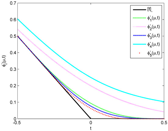
Figure 1. Graphs of ${\left[t\right]}_{-}$ and ${\varphi }_i^{-}(\mu ,t),i=1,2,3,4,5$ with $\mu =0.5$.

From Figure 1, it can be seen that, for a fixed parameter $\mu >0$, function ${\varphi }_3^{-}(\mu ,t)$ is the closest function to ${\left[t\right]}_{-}$ among all ${\varphi }_i^{-}(\mu ,t),i=1,2,3,4,5$. In fact, for a fixed parameter $\mu >0$ and all $t\in \mathrm{I}\mathrm{R}$, we have

$$\begin{array}{c}\hfill {\varphi }_4^{-}(\mu ,t)\ge {\varphi }_2^{-}(\mu ,t)\ge {\varphi }_1^{-}(\mu ,t)\ge {\varphi }_3^{-}(\mu ,t)\ge {\varphi }_5^{-}(\mu ,t)\ge {\left[t\right]}_{-}.\end{array}$$

In this paper, based on the SOC vector-valued function (9), the smooth functions (18)–(22) are applied to the projection function ${(P_{\mathcal{K}}(-y))}^{\sigma }$ in (4) to form a completely smooth lower-order penalty equation, which will be introduced in (27), and then an algorithm is constructed to solve SOCMCP (1).

For any $x=(x_1;\dots ;x_r)\in {\mathrm{I}\mathrm{R}}^{n_1}\times \dots \times {\mathrm{I}\mathrm{R}}^{n_r}$, construct a smoothing function for the projection function $P_{\mathcal{K}}(x),{\overline{P}}_{\mathcal{K}}(x)$ associated with $\mathcal{K}={\mathcal{K}}^{n_1}\times \dots \times {\mathcal{K}}^{n_r}$. First, utilizing the smoothing functions defined by (14) and (16), we will explore the construction of a smoothing function for the projection function $P_{{\mathcal{K}}^{n_i}}(x_i),{\overline{P}}_{{\mathcal{K}}^{n_i}}(x_i)$ related to a single SOC block ${\mathcal{K}}^{n_i}(i=1,\dots ,r)$, where $P_{{\mathcal{K}}^{n_i}}(x_i)$ and ${\overline{P}}_{{\mathcal{K}}^{n_i}}(x_i)$ are given by (10) and (11), respectively. The spectral values and spectral vectors of $x_i\in {\mathrm{I}\mathrm{R}}^{n_i}(i=1,\dots ,r)$ with respect to ${\mathcal{K}}^{n_i}$ are ${\lambda }_1(x_i),{\lambda }_2(x_i)$ and $u_{x_i}^{(1)},u_{x_i}^{(2)}$, respectively. We define a vector-valued function

$$\begin{array}{c}\hfill {\Phi }_i^{+}(\mu ,x_i)={\varphi }^{+}(\mu ,{\lambda }_1(x_i))u_{x_i}^{(1)}+{\varphi }^{+}(\mu ,{\lambda }_2(x_i))u_{x_i}^{(2)},\end{array}$$

(23)

$$\begin{array}{c}\hfill {\Phi }_i^{-}(\mu ,x_i)={\varphi }^{-}(\mu ,{\lambda }_1(x_i))u_{x_i}^{(1)}+{\varphi }^{-}(\mu ,{\lambda }_2(x_i))u_{x_i}^{(2)},\end{array}$$

(24)

where $\mu \in {\mathrm{I}\mathrm{R}}_{++}$ is a smoothing parameter. According to [37], ${\Phi }_i^{+}(\mu ,x_i),{\Phi }_i^{-}(\mu ,x_i)$ is smooth on $\mathrm{I}{\mathrm{R}}_{++}\times {\mathrm{I}\mathrm{R}}^{n_i}$, and 

$$\begin{array}{c}\hfill \underset{\mu \to 0^{+}}{lim}{\Phi }_i^{+}(\mu ,x_i)={\left[{\lambda }_1(x_i)\right]}_{+}{u}_{x_i}^{(1)}+{\left[{\lambda }_2(x_i)\right]}_{+}{u}_{x_i}^{(2)}=P_{{\mathcal{K}}^{n_i}}(x_i),\end{array}$$

$$\begin{array}{c}\hfill \underset{\mu \to 0^{+}}{lim}{\Phi }_i^{-}(\mu ,x_i)={\left[{\lambda }_1(x_i)\right]}_{-}{u}_{x_i}^{(1)}+{\left[{\lambda }_2(x_i)\right]}_{-}{u}_{x_i}^{(2)}={\overline{P}}_{{\mathcal{K}}^{n_i}}(x_i).\end{array}$$

Finally, we construct smooth functions for projection functions $P_{\mathcal{K}}(x)$ and ${\overline{P}}_{\mathcal{K}}(x)$ related to a general cone (2). Define a vector-valued function ${\Phi }^{+},{\Phi }^{-}:\mathrm{I}{\mathrm{R}}_{++}\times {\mathrm{I}\mathrm{R}}^n\to {\mathrm{I}\mathrm{R}}^n$ as

$$\begin{array}{c}\hfill {\Phi }^{+}(\mu ,x)=({\Phi }_1^{+}(\mu ,x_1);\dots ;{\Phi }_r^{+}(\mu ,x_r)),\end{array}$$

(25)

$$\begin{array}{c}\hfill {\Phi }^{-}(\mu ,x)=({\Phi }_1^{-}(\mu ,x_1);\dots ;{\Phi }_r^{-}(\mu ,x_r)),\end{array}$$

(26)

where ${\Phi }_i^{+}(\mu ,x_i),{\Phi }_i^{-}(\mu ,x_i)(i=1,\dots ,r)$ are defined by (23) and (24), respectively. In order to facilitate the proof of subsequent convergence analysis, by [27], Lemma 3.2, we have

$${\Phi }^{+}(\mu ,x)\in \mathcal{K},{\Phi }^{-}(\mu ,x)\in \mathcal{K}.$$

Based on the above smoothing idea, a completely smooth lower-order penalty equation can be established to solve SOCMCP (1). This will be described in the next section.

4. Completely Smooth Lower-Order Penalty Approach and Convergence Analysis

This section will introduce a completely smooth lower-order penalty method for solving SOCMCP (1), and it will also provide a comprehensive convergence analysis. In the following text, unless otherwise specified, $\mathcal{K}$ is always represented as (2). We consider the completely smooth lower-order penalty equations (CSLOPEs)

$$\begin{array}{c}\hfill \left({\displaystyle \genfrac{}{}{0pt}{}{G(x,y)}{F(x,y)}}\right)-\alpha \left({\displaystyle \genfrac{}{}{0pt}{}{0}{{\Phi }^{-}(\mu ,y)}}\right)=0,\end{array}$$

(27)

where $\alpha \ge 1$ is a penalty parameter, $\mu \in (0,1)$ is a smoothing parameter, and ${\Phi }^{-}(\mu ,y)$ is defined as (26). If $y\in \mathcal{K}$ is violated, then the penalty term $\alpha {\Phi }^{-}(\mu ,y)$ in (27) penalizes the ‘negative’ part of y. With a penalty parameter $\alpha \to +\infty$ and a smooth parameter $\mu \to 0^{+}$, it will force y to approach $\mathcal{K}$. In (27), it is straightforward to observe that $F(x,y)\in \mathcal{K}$ always holds because $\alpha {\Phi }^{-}(\mu ,y)\in \mathcal{K}$. We expect the solution sequence of (27) to tend towards the solution of (1). To achieve this, let

$$\begin{array}{c}\hfill \mathbb{F}(x,y)=(G(x,y);F(x,y)),\mathbb{K}=\mathrm{I}{\mathrm{R}}^m\times \mathcal{K},\end{array}$$

(28)

where $\mathcal{K}$ is defined in (2), and let us make the following assumptions.

Assumption 1.

The function $\mathbb{F}(x,y)$ is $\xi$-monotone on $\mathrm{I}{\mathrm{R}}^{m+n}$; i.e., there exist constants $\beta >0$ and $\xi >1$, such that

$$\begin{array}{c}\hfill {((x;y)-(\overline{x};\overline{y}))}^T(\mathbb{F}(x,y)-\mathbb{F}(\overline{x},\overline{y}))\ge \beta {\left|\right|(x;y)-(\overline{x};\overline{y})\left|\right|}^{\xi },\forall (x;y),(\overline{x};\overline{y})\in {\mathrm{I}\mathrm{R}}^{m+n}.\end{array}$$

(29)

It is apparent that a function that is strongly monotonic must also be a $\xi$-monotonic function, though the opposite is not guaranteed. Under Assumption 1, we will undertake an analysis of convergence.

First, we consider the uniqueness of the solutions SOCMCP (1) and CSLOPEs (27). Using Proposition 1.1.3 and Theorem 2.2.3 from [5], Section 3.1 of [29] demonstrates that SOCMCP (1) can be equivalently transformed into a variational inequality. In the case of continuity and $\xi$-monotone, variational inequalities have a unique solution. Therefore, under Assumption 1, SOCMCP (1) is uniquely solvable.

In [30], SLOPEs (5) consider the approximate smooth case of $\sigma \in (0,1]$. In this paper, we further explore the completely smooth case where $\sigma =1$ based on that. Therefore, the remaining results in this section are similar to the propositions and theorems in [30].

Proposition 5.

For any smoothing parameter $\mu \in (0,1)$, the function ${\Phi }^{-}(\mu ,y)$ is defined as (26); then $-{\Phi }^{-}(\mu ,y)$ about y is monotone on $\mathrm{I}{\mathrm{R}}^n$, i.e.,

$$\begin{array}{c}\hfill {(y-y^{\prime })}^T({\Phi }^{-}(\mu ,y)-{\Phi }^{-}(\mu ,y^{\prime }))\le 0,\forall y,y^{\prime }\in {\mathrm{I}\mathrm{R}}^n.\end{array}$$

(30)

According to Proposition 5, for any parameter $\alpha \ge 1,\mu \in (0,1)$, function $-\alpha {\Phi }^{-}(\mu ,y)$ is monotone on $\mathrm{I}{\mathrm{R}}^n$. Suppose that

$$\begin{array}{c}\hfill \Psi (x,y)=\mathbb{F}(x,y)-\alpha (0;({\Phi }^{-}(\mu ,y))).\end{array}$$

(31)

Due to the fact that nonlinear equations can be regarded as unconstrained variational inequalities, the uniqueness solutions of CSLOPEs (27) can be considered through variational inequalities.

Proposition 6.

Under Assumption 1, for any parameter $\alpha \ge 1,\mu \in (0,1)$; then CSLOPEs (27) have a unique solution.

Proposition 7.

For any $\alpha \ge 1$, when μ is sufficiently small, the solution of CSLOPEs (27) is bounded. Specifically, there exists a positive constant M that does not depend on $(x_{\mu ,\alpha };y_{\mu ,\alpha })$, $\mu ,\alpha$, such that $\left|\right|(x_{\mu ,\alpha };y_{\mu ,\alpha })\left|\right|\le M$.

Proposition 8.

For any $\alpha \ge 1$, when μ is sufficiently small, there exists a positive constant C that does not depend on $(x_{\mu ,\alpha };y_{\mu ,\alpha }),\alpha ,\mu$, such that

$$\begin{array}{c}\hfill \left|\right|{\Phi }^{-}(\mu ,y_{\mu ,\alpha })\left|\right|\le {\displaystyle \frac{C}{\alpha }}.\end{array}$$

(32)

Theorem 1.

Suppose that $(x^{*};y^{*})$ is the solution of SOCMCP (1); then for any $\alpha \ge 1$ and sufficiently small μ, $(x_{\mu ,\alpha };y_{\mu ,\alpha })$ is the solution of CSLOPEs (27). Then there exists a positive constant C that does not depend on $(x^{*};y^{*}),(x_{\mu ,\alpha };y_{\mu ,\alpha }),\mu ,\alpha$, such that

$$\begin{array}{c}\hfill \left|\right|(x^{*};y^{*})-(x_{\mu ,\alpha };y_{\mu ,\alpha })\left|\right|\le {\displaystyle \frac{C}{{\alpha }^{1/\xi }}}.\end{array}$$

(33)

5. Algorithm and Numerical Experiments

In this section, we construct a completely smooth lower-order penalty algorithm for solving SOCMCP (1) based on Theorem 1. Additionally, we present several numerical experiments to demonstrate its effectiveness.

Algorithm 1 offers a completely smooth lower-order penalty method for solving SOCMCP (1). In the following sections, we will present several numerical examples to demonstrate the effectiveness of Algorithm 1. In numerical experiments, the smooth functions (18)–(21) are employed, and all nonlinear equations are solved using the smoothing Newton method. For each numerical example, $\mathtt{IP}(x^{(0)};y^{(0)})$ denotes the initial point, $\mathtt{Iter}$ denotes the number of iterations, $\mathtt{CPU}(s)$ records the time taken to calculate the problems, and $\mathtt{Err}$ denotes $\left|\right|(\tilde{x};\tilde{y})-(x^{*};y^{*})\left|\right|$, where $(\tilde{x};\tilde{y})$ denotes the approximate optimal solution obtained through Algorithm 1, and $(x^{*};y^{*})$ denotes the exact solution of the problem. For all subsequent numerical examples presented hereinafter, unless otherwise stated, we adopt a termination criterion of $\mathtt{eps}=1\times {10}^{-6}$. In the numerical experiment table, ‘-’ indicates that the results could not be obtained (due to matrix singularity or other reasons). All the numerical experiments in this paper were run in MATLAB 2012a.

Algorithm 1: Completely Smooth Lower-Order Penalty Algorithm

Step 0 For a continuous differentiable vector-valued function $(G(x,y);F(x,y))$, it is that which satisfies Assumption 1, where $G:{\mathrm{I}\mathrm{R}}^{m+n}\to {\mathrm{I}\mathrm{R}}^m$, $F:{\mathrm{I}\mathrm{R}}^{m+n}\to {\mathrm{I}\mathrm{R}}^n$, and the block form of F is $F=(F_1;\dots ;F_r)$, $F_i:{\mathrm{I}\mathrm{R}}^{m+n}\to {\mathrm{I}\mathrm{R}}^{n_i}(i=1,\dots ,r)$, and the block form of variable y is $y=(y_1;\dots ;y_r)$, $y_i\in {\mathrm{I}\mathrm{R}}^{n_i}(i=1,\dots ,r)$. Setting $(\tilde{x};\tilde{y})=0$$\in {\mathrm{I}\mathrm{R}}^{m+n}$. Step 1 If $G(0)=0$, $F(0)\in \mathcal{K}$, go to step5; else, go to step2. Step 2 For the penalty parameter $\alpha \ge 1$, the smoothing parameter $\mu \in (0,1)$, the error bound $\mathtt{eps}$, and the multiple parameters $c_1>1$ and $c_2<1$, select an initial point $(x^{(0)};y^{(0)})$, where $y^{(0)}=(y_1^{(0)};\dots ;y_r^{(0)})\in {\mathrm{I}\mathrm{R}}^{n_1}\times \dots \times {\mathrm{I}\mathrm{R}}^{n_r}$ with $y_i^{(0)}=(y_{i1}^{(0)};y_{i2}^{(0)})\in \mathrm{I}\mathrm{R}\times {\mathrm{I}\mathrm{R}}^{n_i-1}(i=1,\dots ,r)$ by taking $y_{i2}^{(0)}\ne 0$ while $y_{i1}^{(0)}<0$. Step 3 For the parameters $\alpha ,\mu$ and the initial point $(x^{(0)};y^{(0)})$, solve the nonlinear equations $$(G(x,y);F(x,y))-\alpha (0;{\Phi }^{-}(\mu ,y))=0;$$ setting $(x_{\mu ,\alpha };y_{\mu ,\alpha })$ denotes the solution of this nonlinear equations. Let $$\mathtt{Tol}=|y_{\mu ,\alpha }^{T}F(x_{\mu ,\alpha },y_{\mu ,\alpha })|+||G(x_{\mu ,\alpha },y_{\mu ,\alpha })\left|\right|.$$ Step 4 If $\mathtt{Tol}\le \mathtt{eps}$, set $(\tilde{x};\tilde{y})=(x_{\mu ,\alpha };y_{\mu ,\alpha })$, go to step5; else, let $(x^{(0)};y^{(0)})=$$(x_{\mu ,\alpha };y_{\mu ,\alpha })$, $\alpha =c_1\alpha$, and $\mu =c_2\mu$, go to step3. Step 5 The vector $(\tilde{x};\tilde{y})$ serves as the approximate optimal solution for SOCMCP (1); stop.

Example 1.

Consider SOCMCP (1) on ${\mathcal{K}}^3$, where $x\in \mathrm{I}\mathrm{R}$, $y={(y_1,y_2,y_3)}^T\in {\mathcal{K}}^3$ and

$$G(x,y)=x+2y_1-2y_2-y_3-2=0,F(x,y)=\left(\begin{array}{c}0.07y_1^3-4\\ 0.04y_2^3-3.93\\ 0.03y_3^3-5.72\end{array}\right)\in {\mathcal{K}}^3.$$

This example is derived from [29]. The function $G(x,y)$ is a linear function, and $F(x,y)$ is $\xi$-monotonic but not strongly monotonic due to $F(x,y)$, which is composed of a cubic term and a constant term. According to [29], the precise solution for Example 1 is $x^{*}=2,y^{*}={(5,3,4)}^T$. The effect of individual parameter $\mu ,\alpha$ changes on the numerical results is considered below. Taking the initial point $(x^{(0)};y^{(0)})={(1,1,1,1)}^T$, the numerical experiments were conducted following these two distinct steps:

• First, we set $\mu =1\times {10}^{-5}$ and consider various values $\alpha =70\times 7^i,i=1,\dots ,6$. The corresponding numerical results are presented in Table 1.
  Table 1. The numerical results corresponding to variations in $\alpha$ ($\mu =1\times {10}^{-4}$).

  $\mathit{\alpha }\to$		490	3430	24,010	168,070	1,176,490	8,235,430
  ${\varphi }_1^{-}$	Val	−0.0913	−0.0131	−0.0019	−2.5852 $\times {10}^{-4}$	1.2631 $\times {10}^{-4}$	2.9902 $\times {10}^{-4}$
  	Err	0.0429	0.0062	8.7999 $\times {10}^{-4}$	1.2106 $\times {10}^{-4}$	5.9144 $\times {10}^{-5}$	1.4002 $\times {10}^{-4}$
  ${\varphi }_2^{-}$	Val	−0.0913	−0.0131	−0.0019	−1.4133 $\times {10}^{-4}$	4.8279 $\times {10}^{-4}$	8.9470 $\times {10}^{-4}$
  	Err	0.0429	0.0062	8.7998 $\times {10}^{-4}$	6.6178 $\times {10}^{-5}$	2.2607 $\times {10}^{-4}$	4.1895 $\times {10}^{-4}$
  ${\varphi }_3^{-}$	Val	−0.0913	−0.0131	−0.0019	−2.6365 $\times {10}^{-4}$	8.3499 $\times {10}^{-5}$	2.5553 $\times {10}^{-4}$
  	Err	0.0429	0.0062	8.7999 $\times {10}^{-4}$	1.2346 $\times {10}^{-4}$	3.9100 $\times {10}^{-5}$	1.1965 $\times {10}^{-4}$
  ${\varphi }_4^{-}$	Val	−0.0913	−0.0131	−0.0018	1.5169 $\times {10}^{-4}$	0.0029	0.0206
  	Err	0.0429	0.0062	8.6625 $\times {10}^{-4}$	3.0870 $\times {10}^{-5}$	6.5788 $\times {10}^{-4}$	0.0047

• Second, we set $\alpha =490$ and consider various values $\mu =0.5,0.2,0.1,0.01,0.001,0.0001$. The corresponding numerical results are presented in Table 2,
  Table 2. The numerical results corresponding to variations in $\mu$ ($\alpha =490$).

  $\mathit{\mu }\to$		0.5	0.2	0.1	0.01	0.001	0.0001
  ${\varphi }_1^{-}$	Val	1.0572	0.2044	−0.0060	−0.0913	−0.0913	−0.0913
  	Err	0.4736	0.0948	0.0028	0.0429	0.0429	0.0429
  ${\varphi }_2^{-}$	Val	3.5424	0.8866	0.2429	−0.0908	−0.0913	−0.0913
  	Err	1.4652	0.3999	0.1125	0.0427	0.0429	0.0429
  ${\varphi }_3^{-}$	Val	0.8110	0.1225	−0.0354	−0.0913	−0.0913	−0.0913
  	Err	0.3669	0.0570	0.0166	0.0429	0.0429	0.0429
  ${\varphi }_4^{-}$	Val	30.3779	4.7832	1.1272	−0.0791	−0.0912	−0.0913
  	Err	4.2871	0.9511	0.2288	0.0401	0.0429	0.0429

where $\mathtt{Val}$ denotes $y_{\mu ,\alpha }^{T}F(x_{\mu ,\alpha },y_{\mu ,\alpha })$ in Table 1 and Table 2.

From these tables, we can draw the following conclusions:

• In Table 1, as the penalty parameter $\alpha$ increases, Err gradually decreases. When employing ${\varphi }_i^{-}(i=1,2,3,4)$ for solving the problem, the value of Val transitions from negative to positive. For instance, when utilizing ${\varphi }_4^{-}$ to solve, the penalty parameter $\alpha$ increases to 168,070; we observed that Val shifts from a negative to a positive value. This indicates that the penalty parameter $\alpha =$ 168,070 is already large enough, and simply increasing its value will not yield better results. At this juncture, it becomes essential to consider adopting a smaller smoothing parameter $\mu$.
• In Table 2, as the smoothing parameter $\mu$ decreases, the overall trend of $\mathtt{Err}$ exhibits a gradual decline. However, the subsequent changes are not significant, primarily due to the simple reduction in the smoothing parameter $\mu$, without taking into account the influence of penalty parameters on numerical calculations. For instance, when employing ${\varphi }_2^{-}$ for solving purposes, the value of the smoothing parameter $\mu$ changes from 0.1 to 0.01; $\mathtt{Val}$ changes from positive to negative. This indicates that the smoothing parameter $\mu =0.01$ is sufficiently small; thus further reductions will not yield improved outcomes. In fact, what is truly required at this point is an increase in the penalty parameter $\alpha$.

In Example 1, a fixed initial point was chosen to investigate the influence of various parameters on numerical experiments. In fact, when different initial points are employed, the numerical outcomes remain consistent with those presented in Table 1 and Table 2. Thus, we will not reiterate them here. The subsequent example serves to illustrate the effects of varying initial points on the numerical results.

Example 2.

For nonlinear SOCP with convex objective functions

$$\begin{array}{cc}\hfill \mathit{min}& x_1^2+2x_2^2+2x_1{x}_2-10x_1-12x_2,\hfill \\ \hfill s.t.& \left(\begin{array}{c}8-x_1+3x_2\\ 3-x_1^2-2x_1-x_2^2+2x_2\end{array}\right)\in {\mathcal{K}}^2,\hfill \end{array}$$

the KKT condition is

$$y\in {\mathcal{K}}^2,F(x,y)\in {\mathcal{K}}^2,y^{T}F(x,y)=0,G(x,y)=0,$$

where $x={(x_1,x_2)}^T,y={(y_1,y_2)}^T$,

$$F(x,y)=\left(\begin{array}{c}8-x_1+3x_2\\ 3-x_1^2-2x_1-x_2^2+2x_2\end{array}\right),G(x,y)=\left(\begin{array}{c}2x_1+2x_2-10+y_1+2(x_1+1)y_2\\ 2x_1+4x_2-12-3y_1+2(x_2-1)y_2\end{array}\right).$$

This example is derived from [29]. According to [29], the approximate optimal solution for Example 2 is $(\tilde{x};\tilde{y})\approx {(2.830835,1.637521,0.122758,0.122758)}^T$. When applying different initial points, by taking $c_1=10$, $c_2=0.1$, initial $\alpha =1000$, and proper initial $\mu =1\times {10}^{-6}$, the test results are summarized in Table 3. From Table 3, it can be seen that, for all initial points listed in the table, Example 2 can be solved by using Algorithm 1, which indicates that Algorithm 1 is not very sensitive to the initial points.

Table 3. The numerical results with different initial points ($\mu =1\times {10}^{-6},\alpha =1000$).

IP$({\mathit{x}}^{(0)};{\mathit{y}}^{(0)})$	Val$({\mathit{\varphi }}_1)$	Val$({\mathit{\varphi }}_2)$	Val$({\mathit{\varphi }}_3)$	Val$({\mathit{\varphi }}_4)$
(2,1,0,1)	-	2.0256 $\times {10}^{-7}$	-	2.0347 $\times {10}^{-7}$
${10}^{-2}$(1,1,0,1)	2.0349 $\times {10}^{-7}$	2.0384 $\times {10}^{-7}$	2.0288 $\times {10}^{-7}$	2.0251 $\times {10}^{-7}$
${10}^{12}$(2,2,1,1)	-	2.0268 $\times {10}^{-7}$	2.0367 $\times {10}^{-7}$	2.0300 $\times {10}^{-7}$
−${10}^{-3}$(2,1,0,1)	2.0366 $\times {10}^{-7}$	2.0256 $\times {10}^{-7}$	2.0348 $\times {10}^{-7}$	2.0300 $\times {10}^{-7}$
$-(2\times {10}^5,{10}^3,2\times {10}^6,1\times {10}^4)$	2.0264 $\times {10}^{-7}$	2.0347 $\times {10}^{-7}$	2.0348 $\times {10}^{-7}$	2.0391 $\times {10}^{-7}$

In the aforementioned numerical experiment, the smooth functions (18)–(21) were utilized. However, which smooth function has better numerical performance? That is to say, it is imperative to conduct a comparative analysis of the performance among the functions ${\varphi }_i^{-}(\mu ,t)(i=1,2,3,4,5)$. For this purpose, we employ the performance profile method, as introduced in [38], to evaluate and compare the performances of these functions.

Assuming that there are $n_s$ solvers from the solver set $\mathcal{S}$ and $n_p$ test problems from the test set $\mathcal{P}$, we use computation time and the number of iterations as performance metrics. Here, we adopt computation time as the primary measure. For each problem p and solver s, define

$$f_{p,s}=\mathrm{computing} \mathrm{time} \mathrm{required} \mathrm{to} \mathrm{solve} \mathrm{problem} p \mathrm{by} \mathrm{solver} s,$$

and utilize the performance ratio

$$r_{p,s}={\displaystyle \frac{f_{p,s}}{min\left\{f_{p,s}|s\in \mathcal{S}\right\}}}.$$

Assuming a parameter $r_M$ is selected such that $r_{p,s}\le r_M$ for all $p,s$, with $r_{p,s}=r_M$ if and only if solver s fails to solve problem p. The selection of $r_M$ does not influence the performance evaluation. To gain a comprehensive evaluation for each solver, we define

$${\rho }_s(\tau )={\displaystyle \frac{1}{n_p}}\mathrm{size}\left\{p\in \mathcal{P}|r_{p,s}\le \tau \right\}.$$

The function ${\rho }_s(\tau )$ represents the cumulative performance ratio, also referred to as the performance profile.

According to [30], ${\varphi }_5^{-}(\mu ,t)$ is the smooth function with the best performance. To compare the effectiveness of the smooth functions ${\varphi }_i^{-}(\mu ,t)(i=1,2,3,4)$ proposed in this paper with ${\varphi }_5^{-}(\mu ,t)$ from [30], we will consider two numerical examples, which belong to SOCP with both equality and inequality constraints and SOCP with inequality constraint. For the performance profile, the smooth functions ${\varphi }_i^{-}(\mu ,t)(i=1,2,3,4,5)$ from (18)–(22) are treated as five solvers. Additionally, 20 initial points are randomly generated as 20 test problems to evaluate the performance of these solvers on the numerical examples.

Example 3.

Consider nonlinear SOCP with equality and inequality constraints, and convex objective functions

$$\begin{array}{cc}\hfill \mathit{min}& f(z)=\mathit{exp}({(z_1-3)}^2+z_2^2+{(z_3-1)}^2+{(z_4-2)}^2+{(z_5+2)}^2),\hfill \\ \hfill s.t.& \left\{\begin{array}{c}h(z)=z_1+2z_2+3z_3-3z_4-z_5-2=0,\hfill \\ g(z)=z\in {\mathcal{K}}^5,\hfill \end{array}\right.\hfill \end{array}$$

where $z={(z_1,z_2,z_3,z_4,z_5)}^T$. The KKT conditions of this SOCP can be transformed into the following SOCMCP:

$$y={(y_1,y_2,y_3,y_4,y_5)}^T\in {\mathcal{K}}^5,$$

$$F(x,y)=2f(y){(y_1-3,y_2,y_3-1,y_4-2,y_5+2)}^T-x{(1,2,3,-3,-1)}^T\in {\mathcal{K}}^5,$$

$$y^{T}F(x,y)=0,x\in \mathrm{I}\mathrm{R},G(x,y)=y_1+2y_2+3y_3-3y_4-y_5-2=0.$$

This example is derived from [29]. According to [29], the exact optimal solution for Example 3 is $x^{*}=0,y^{*}={(3,0,1,2,-2)}^T$. Randomly selecting 20 initial points, by taking $c_1=10$, $c_2=0.1$, initial $\alpha =1000$, and initial $\mu =1\times {10}^{-6}$, the performance profile based on calculation time is shown in Figure 2.

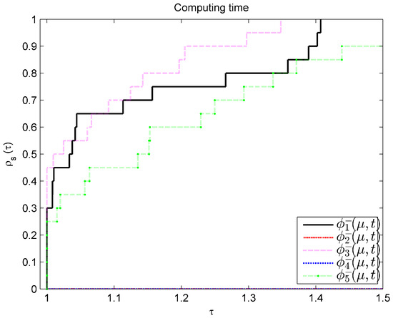
Figure 2. Performance profile of ${\varphi }_i^{-}(\mu ,t),i=1,2,3,4,5$ for Example 3.

Example 4.

Consider the following nonlinear SOCP:

$$\begin{array}{cc}\hfill \mathit{min}& \mathit{exp}(x_1-x_2)+{(x_1-x_5)}^4+{\displaystyle \frac{1}{2}}{\left|\right|x\left|\right|}^2-\sum _{i=1}^5{x}_i,\hfill \\ \hfill s.t.& \left(\begin{array}{c}{x}^{T}Mx+c^{T}x+m\\ Ax-b\end{array}\right)\in {\mathcal{K}}^n,\hfill \end{array}$$

where $x={(x_1,x_2,x_3,x_4,x_5)}^T,n=4,m=1$ and

$$\begin{array}{c}\hfill M=\left[\begin{array}{ccccc}-0.0534& 0.2689& 0.3987& 0.5193& -0.1132\\ 0.2689& -0.4283& -0.1669& -0.1164& -0.4574\\ 0.3987& -0.1669& -0.8921& 0.0996& 0.5735\\ 0.5193& -0.1164& 0.0996& -0.0612& -0.6769\\ -0.1132& -0.4574& 0.5735& -0.6769& 0.0571\end{array}\right],\end{array}$$

$$\begin{array}{c}\hfill A=\left[\begin{array}{ccccc}-0.6687& 0.3082& -0.0989& 0.8267& 0.0767\\ 0.2040& 0.3784& -0.8324& -0.6952& 0.9923\\ -0.4741& 0.4963& -0.5420& 0.6516& -0.8436\end{array}\right],\end{array}$$

$$\begin{array}{c}\hfill c={(-0.1146,-0.7867,0.9238,-0.9907,0.5498)}^T,b={(0.6346,0.7374,-0.8311)}^T.\end{array}$$

Let $y={(y_1,y_2,y_3,y_4)}^T$; then the KKT conditions for the above SOCP is SOCMCP, as follows:

$$\begin{array}{c}\hfill y\in {\mathcal{K}}^4,F(x,y)\in {\mathcal{K}}^4,y^{T}F(x,y)=0,G(x,y)=0,\end{array}$$

where

$$\begin{array}{c}\hfill F(x,y)=\left(\begin{array}{c}{x}^{T}Mx+c^{T}x+1\\ Ax-b\end{array}\right),\end{array}$$

$$\begin{array}{c}\hfill G(x,y)=\left(\begin{array}{c}\mathit{exp}(x_1-x_2)+4{(x_1-x_5)}^3+x_1-1\\ -\mathit{exp}(x_1-x_2)+x_2-1\\ x_3-1\\ x_4-1\\ -4{(x_1-x_5)}^3+x_5-1\end{array}\right)-{\left(\begin{array}{c}{(2Mx+c)}^T\\ A\end{array}\right)}^{T}y=0.\end{array}$$

This example is derived from [33]. According to [33], the approximate optimal solution for Example 4 is $(\tilde{x};\tilde{y})\approx (0.69393,0.87434,1.00356,0.40226,1.06616,0.49209,0.38664,$ ${0.24221,0.18440)}^T$. Randomly selecting 20 initial points, by taking $c_1=10$, $c_2=0.1$, initial $\alpha =1000$, and initial $\mu =1\times {10}^{-8}$, the performance profile based on calculation time is shown in Figure 3.

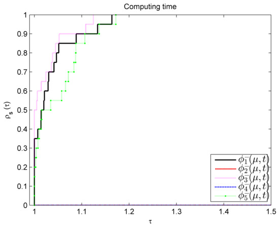
Figure 3. Performance profile of ${\varphi }_i^{-}(\mu ,t),i=1,2,3,4,5$ for Example 4.

In [33], $M\in {\mathbb{S}}^5$, $A\in \mathrm{I}{\mathrm{R}}^{(n-1)\times 5}$, $c\in \mathrm{I}{\mathrm{R}}^5$, $b\in \mathrm{I}{\mathrm{R}}^{n-1}$, and $m\in \mathrm{I}\mathrm{R}$. Randomly selecting $M,A,c,b,m$ and 20 initial points, by taking $c_1=10$, $c_2=0.1$, initial $\alpha =800$, and initial $\mu =1\times {10}^{-8}$, the performance profile based on calculation time is shown in Figure 4.

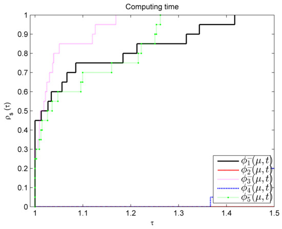
Figure 4. Performance profile of ${\varphi }_i^{-}(\mu ,t),i=1,2,3,4,5$ for Example 4.

From Figure 2, Figure 3 and Figure 4, it is evident that ${\varphi }_3^{-}(\mu ,t)$ exhibits the best performance, followed by ${\varphi }_1^{-}(\mu ,t)$ and then ${\varphi }_5^{-}(\mu ,t)$. Under the parameter selection of Examples 3 and 4, ${\varphi }_2^{-}(\mu ,t)$ and ${\varphi }_4^{-}(\mu ,t)$ cannot be solved well. Therefore, when using Algorithm 1 to solve SOCMCP, the smooth function ${\varphi }_3^{-}(\mu ,t)$ is the best choice.

In [30], the smooth-like lower-order penalty equations (SLOPEs) algorithm transforms SOCMCP (1) into smooth-like lower-order penalty equations (5) with smooth functions. We attempt to use the smooth Newton method to solve nonlinear equations when the SLOPEs index $\sigma \in (0,1]$. In Algorithm 1 of this paper, the projection function ${\left[t\right]}_{-}$ is approximated by the smooth functions ${\varphi }_i^{-}(\mu ,t)(i=1,2,3,4,5)$, and ${\varphi }_3^{-}(\mu ,t)$ is the best choice. Therefore, the performance of Algorithm 1 is compared with that of SLOPEs below, especially using the best smooth function ${\varphi }_3^{-}(\mu ,t)$.

Examples 2–4 are numerical examples that satisfy Assumption 1. In Algorithm 1 and SLOPEs, we take $c_1=10$, $c_2=0.1$, initial $\alpha =100$, and initial $\mu =1\times {10}^{-7}$. In SLOPEs, we take $\sigma =1$. The numerical performance comparison results for different termination criteria are shown in Table 4.

Table 4. Comparison results of the value of $\mathtt{Val}$.

Example	IP$({\mathit{x}}^{(0)};{\mathit{y}}^{(0)})$	eps	Algorithm 1 (${\mathit{\varphi }}_3^{-}$)			SLOPEs (${\mathit{\varphi }}_3^{-}$)
			Val	Iter	CPU (s)	Val	Iter	CPU (s)
Example 2	(2,1,0,1)	1 $\times {10}^{-6}$	2.0348 $\times {10}^{-7}$	8	0.6840	2.0349 $\times {10}^{-7}$	8	0.7050
		1 $\times {10}^{-7}$	2.4119 $\times {10}^{-8}$	9	0.6825	-	-	-
		1 $\times {10}^{-8}$	-	-	-	-	-	-
Example 3	(1,0,1,0,1,0)	1 $\times {10}^{-6}$	8.8526 $\times {10}^{-15}$	1	0.8787	8.8526 $\times {10}^{-15}$	1	0.8837
		1 $\times {10}^{-7}$	8.8526 $\times {10}^{-15}$	1	0.8604	8.8526 $\times {10}^{-15}$	1	0.8966
		1 $\times {10}^{-8}$	8.8526 $\times {10}^{-15}$	1	0.8973	8.8526 $\times {10}^{-15}$	1	0.9150
Example 4	(1,1,1,1,1,1,1,1,1)	1 $\times {10}^{-6}$	8.5625 $\times {10}^{-7}$	5	1.0551	8.5625 $\times {10}^{-7}$	5	1.1108
		1 $\times {10}^{-7}$	8.5450 $\times {10}^{-8}$	6	1.1771	8.5450 $\times {10}^{-8}$	6	1.2106
		1 $\times {10}^{-8}$	8.1203 $\times {10}^{-9}$	7	1.2264	8.1203 $\times {10}^{-9}$	7	1.2755

It can be concluded from Table 4 that, in the case of ${\varphi }_3^{-}(\mu ,t)$, Algorithm 1 has better numerical performance than the SLOPEs, which is mainly reflected in the following two aspects: (1) From the termination criteria, Algorithm 1 has higher accuracy than the SLOPEs. When the termination criterion is $1\times {10}^{-7}$, Example 2 can be solved by Algorithm 1, but cannot be solved using SLOPEs. Therefore, for more refined termination criteria, Algorithm 1 can be calculated. (2) Under the same termination criteria that can be solved, Algorithm 1 has a slight advantage over SLOPEs in iteration time. Algorithm 1 parameterizes the power to 1 on the basis of SLOPEs, further smoothing the SLOPEs. SLOPEs added a criterion to determine whether the iteration point is within the second-order cone in the algorithm steps, while Algorithm 1 simplifies this step to make the algorithm more concise. According to the results in Table 4, there is no significant difference between the values of Val of the two algorithms. From this point of view, Algorithm 1 does have better numerical performance than SLOPEs.

The numerical comparisons above are based on termination criteria. Since Examples 1 and 3 have exact solutions, the numerical performances of Algorithm 1 and SLOPEs are compared by using the distance between the numerical solutions and the exact solutions as a new termination criterion. The new termination criterion for both algorithms is set to $1\times {10}^{-6}$. In Algorithm 1 and SLOPEs, all take $c_1=10$, $c_2=0.1$, initial $\alpha =100$, and initial $\mu =1\times {10}^{-7}$. In the SLOPEs, take $\sigma$ as 1. Numerical performance comparison results are shown in Table 5. From the degree to which the numerical solution is close to the exact solution, it can be seen that Algorithm 1 has better numerical performance than SLOPEs.

Table 5. Comparison results of the value of $\mathtt{Err}$.

Example	IP$({\mathit{x}}^{(0)};{\mathit{y}}^{(0)})$	Algorithm 1 (${\mathit{\varphi }}_3^{-}$)			SLOPEs (${\mathit{\varphi }}_3^{-}$)
		Err	Iter	CPU (s)	Err	Iter	CPU (s)
Example 1	(1,1,1,1)	2.1163 $\times {10}^{-7}$	7	0.7527	2.1220 $\times {10}^{-7}$	7	0.7827
Example 3	(1,0,1,0,1,0)	3.3346 $\times {10}^{-8}$	1	0.8787	3.3346 $\times {10}^{-8}$	1	0.8837

The functions in Examples 1–4 all satisfy Assumption 1 or nearly so. The following example will attempt to solve SOCP with a non-convex objective function.

Example 5.

Consider nonlinear SOCP

$$\begin{array}{cc}\hfill \mathit{min}& f(x)=e^{x_1{x}_3}+3{(x_1+x_2)}^2-\sqrt{1+{(2x_2-x_3)}^2}+{\displaystyle \frac{1}{2}}{x}_4^2+{\displaystyle \frac{1}{2}}{x}_5^2,\hfill \\ \hfill s.t.& \left\{\begin{array}{c}h(x)=-24.51x_1+58x_2-16.67x_3-x_4-3x_5+11=0,\hfill \\ g_1(x)=\left(\begin{array}{c}3x_1^3+2x_2-x_3+5x_3^2\\ -5x_1^3+4x_2-2x_3+10x_3^3\\ x_3\end{array}\right)\in {\mathcal{K}}^3,\hfill \\ g_2(x)=\left(\begin{array}{c}{x}_4\\ 3x_5\end{array}\right)\in {\mathcal{K}}^2.\hfill \end{array}\right.\hfill \end{array}$$

The KKT conditions of this SOCP are the following SOCMCP:

$$y\in {\mathcal{K}}^3\times {\mathcal{K}}^2,F(x,y)\in {\mathcal{K}}^3\times {\mathcal{K}}^2,y^{T}F(x,y)=0,G(x,y)=0,$$

where $y={(y_1,y_2,y_3,y_4,y_5)}^T,x={(x_1,x_2,x_3,x_4,x_5,x_6)}^T$,

$$\begin{array}{c}\hfill F(x,y)=\left(\begin{array}{c}3x_1^3+2x_2-x_3+5x_3^2\\ -5x_1^3+4x_2-2x_3+10x_3^3\\ x_3\\ x_4\\ 3x_5\end{array}\right),\end{array}$$

$$\begin{array}{c}\hfill G(x,y)=\left(\begin{array}{c}{x}_3{e}^{x_1{x}_3}+6(x_1+x_2)-9x_1^2{y}_1+15x_1^2{y}_2+24.51x_6\\ 6(x_1+x_2)-{\displaystyle \frac{2(2x_2-x_3)}{\sqrt{1+{(2x_2-x_3)}^2}}}-2y_1-4y_2-58x_6\\ x_1{e}^{x_1{x}_3}+{\displaystyle \frac{2x_2-x_3}{\sqrt{1+{(2x_2-x_3)}^2}}}-(10x_3-1)y_1-(30x_3^2-2)y_2-y_3+16.67x_6\\ x_4-y_4+x_6\\ x_5-3y_5+3x_6\\ -24.51x_1+58x_2-16.67x_3-x_4-3x_5+11\end{array}\right).\end{array}$$

This example is derived from [34]. Since the objective function of the nonlinear SOCP is non-convex, $(G(x,y);F(x,y))$ does not satisfy $\xi$-monotonicity. For different initial points, we attempt to solve Example 5 using Assumption 1 with ${\varphi }_3^{-}$, taking $c_1=10$, $c_2=0.1$, initial $\alpha =100$, and initial $\mu =1\times {10}^{-7}$. For the initial points ${10}^4{(1,1,1,0,1,1,1,0,1,1,1)}^T$ or ${10}^{-7}{(1,1,1,1,1,0,1,0,1,0,1)}^T$, the approximate optimal solution is $(0.12916,-0.11255,-0.06336,0.00957,0.00957,-0.09046,-0.04491,$ 0.63661${,0,0,0.00957)}^T$, which is consistent with the computational results in [34]. However, for the initial points $-{10}^4{(1,1,1,1,1,0,1,0,1,0,1)}^T$ or ${(1,1,1,1,1,1,0,1,0,1,0)}^T$, the numerical solution is $(5.32406,5.17849,-1.23647,0.38361,-0.38361,0.51653,0.09572,$ 0.12991${,0.86311,0.28770,-0.47951)}^T$. It can be observed that this solution is also a local optimal solution of the original SOCP. This indicates that Assumption 1 is also applicable to some SOCMCPs that are not $\xi$-monotone.

6. Conclusions

Based on the completely smooth lower-order penalty equations (CSLOPEs) (27), this paper proposes a completely smooth lower-order penalty method for solving SOCMCP (1). As the main result, Theorem 1 proves that, under Assumption 1, the solution sequence of CSLOPEs (27) converges to the solution of SOCMCP (1) at an exponential rate. In the numerical experiments, five smooth functions corresponding to ${\varphi }_i^{-}(\mu ,t),i=1,2,3,4,5$ are considered. The numerical experimental results show that ${\varphi }_3^{-}(\mu ,t)$ has better numerical performance. Meanwhile, the accuracy of Algorithm 1 is generally higher than that of SLOPEs, and Algorithm 1 is also applicable to some SOCMCPs without Assumption 1.

References

- Hayashi, S.; Yamashita, N.; Fukushima, M. A combined smoothing and regularization method for monotone second-order cone complementarity problems. Siam J. Optim. 2005, 15, 593–615. [Google Scholar] [CrossRef]
- Fukushima, M.; Luo, Z.Q.; Tseng, P. Smoothing functions for second-order-cone complementarity problems. Siam J. Optim. 2002, 12, 436–460. [Google Scholar] [CrossRef]
- Lobo, M.S.; Vandenberghe, L.; Boyd, S.; Lebret, H. Applications of second order cone programming. Linear Algebra Its Appl. 1998, 284, 193–228. [Google Scholar] [CrossRef]
- Alizadeh, F.; Goldfarb, D. Second-order cone programming. Math. Program. 2003, 95, 3–51. [Google Scholar] [CrossRef]
- Facchinei, F.; Pang, J.S. Finite-Dimensional Variational Inequalities and Complementarity Problems; Springer: New York, NY, USA, 2003. [Google Scholar]
- Wilmott, P.; Dewynne, J.; Howison, S. Option Pricing: Mathematical Model and Computation; Oxford Financial Press: Oxford, UK, 1993. [Google Scholar]
- Monteiro, R.D.C.; Tsuchiya, T. Polynomial convergence of primal–dual algorithms for the second-order cone programs based on the MZ-family of directions. Math. Program. 2000, 88, 61–83. [Google Scholar] [CrossRef]
- Chen, X.D.; Sun, D.; Sun, J. Complementarity functions and numerical experiments for second-order cone complementarity problems. Comput. Optim. Appl. 2003, 25, 39–56. [Google Scholar] [CrossRef]
- Huang, Z.H.; Ni, T. Smoothing algorithms for complementarity problems over symmetric cones. Comput. Optim. Appl. 2010, 45, 557–579. [Google Scholar] [CrossRef]
- Kanzow, C.; Ferenczi, I.; Fukushima, M. On the local convergence of semismooth Newton methods for linear and nonlinear second-order cone programs without strict complementarity. Siam J. Optim. 2009, 20, 297–320. [Google Scholar] [CrossRef]
- Pan, S.; Chen, J.S. A damped Gauss-Newton method for the second-order cone complementarity problem. Appl. Math. Optim. 2009, 59, 293–318. [Google Scholar] [CrossRef]
- Hayashi, S.; Yamaguchi, T.; Yamashita, N.; Fukushima, M. A matrix-splitting method for symmetric affine second-order cone complementarity problems. J. Comput. Appl. Math. 2005, 175, 335–353. [Google Scholar] [CrossRef]
- Zhang, L.H.; Yang, W.H. An efficient matrix splitting method for the second-order cone complementarity problem. Siam J. Optim. 2014, 24, 1178–1205. [Google Scholar] [CrossRef]
- Chen, J.S.; Tseng, P. An unconstrained smooth minimization reformulation of the second-order cone complementarity problem. Math. Program. 2005, 104, 293–327. [Google Scholar] [CrossRef]
- Chen, J.S. Two classes of merit functions for the second-order cone complementarity problem. Math. Methods Oper. Res. 2006, 64, 495–519. [Google Scholar] [CrossRef]
- Chen, J.S.; Pan, S. A descent method for a reformulation of the second-order cone complementarity problem. J. Comput. Appl. Math. 2008, 213, 547–558. [Google Scholar] [CrossRef]
- Di Pillo, G.; Grippo, L. An exact penalty function method with global convergence properties for nonlinear programming problems. Math. Program. 1986, 36, 1–18. [Google Scholar] [CrossRef]
- Zangwill, W.I. Nonlinear programming via penalty functions. Manag. Sci. 1967, 13, 344–358. [Google Scholar] [CrossRef]
- Han, S.P.; Mangasarian, O.L. Exact penalty functions in nonlinear programming. Math. Program. 1979, 17, 251–269. [Google Scholar] [CrossRef]
- Bertsekas, D.; Nedić, A.; Ozdaglar, A. Convex Analysis and Optimization; Athena Scientific: Belmont, MA, USA, 2003. [Google Scholar]
- Wang, S.; Yang, X. A power penalty method for linear complementarity problems. Oper. Res. Lett. 2008, 36, 211–214. [Google Scholar] [CrossRef]
- Huang, C.; Wang, S. A power penalty approach to a nonlinear complementarity problem. Oper. Res. Lett. 2010, 38, 72–76. [Google Scholar] [CrossRef]
- Huang, C.; Wang, S. A penalty method for a mixed nonlinear complementarity problem. Nonlinear-Anal.-Theory Methods Appl. 2012, 75, 588–597. [Google Scholar] [CrossRef]
- Hao, Z.; Wan, Z.; Chi, X. A power penalty method for second-order cone linear complementarity problems. Oper. Res. Lett. 2015, 43, 137–142. [Google Scholar] [CrossRef]
- Hao, Z.; Wan, Z.; Chi, X.; Chen, J. A power penalty method for second-order cone nonlinear complementarity problems. J. Comput. Appl. Math. 2015, 290, 136–149. [Google Scholar] [CrossRef]
- Chen, C.; Mangasarian, O.L. A class of smoothing functions for nonlinear and mixed complementarity problems. Comput. Optim. Appl. 1996, 5, 97–138. [Google Scholar] [CrossRef]
- Hao, Z.; Nguyen, C.T.; Chen, J.S. An approximate lower order penalty approach for solving second-order cone linear complementarity problems. J. Glob. Optim. 2022, 83, 671–697. [Google Scholar] [CrossRef]
- Chieu, T.N.; Jan, H.A.; Hao, Z.; Chen, J.S. Smoothing penalty approach for solving second-order cone complementarity problems. J. Glob. Optim. 2025, 91, 39–58. [Google Scholar]
- Hao, Z.; Wan, Z.; Chi, X.; Jin, Z.F. Generalized lower-order penalty algorithm for solving second-order cone mixed complementarity problems. J. Comput. Appl. Math. 2021, 385, 113168. [Google Scholar] [CrossRef]
- Hao, Z.; Wu, Q.; Zhao, C. Smooth-like lower order penalty approach for solving second-order cone mixed complementarity problems. J. Comput. Appl. Math. 2024, 91, 39–58. [Google Scholar]
- Nguyen, C.T.; Saheya, B.; Chang, Y.L. Unified smoothing functions for absolute value equation associated with second-order cone. Appl. Numer. Math. 2019, 135, 206–227. [Google Scholar] [CrossRef]
- Yong, L.Q. Uniformly smooth approximation function and its properties. J. Shaanxi Univ. Technol. (Natural Sci. Ed.) 2018, 34, 74–79. (In Chinese) [Google Scholar]
- Okuno, T.; Yasuda, K.; Hayashi, S. SL1QP Based algorithm with trust region technique for solving nonlinear second-order cone programming problems. Interdiscip. Inf. Sci. 2015, 21, 97–107. [Google Scholar]
- Miao, X.; Chen, J.S.; Ko, C.H. A smoothed NR neural network for solving nonlinear convex programs with second-order cone constraints. Inf. Sci. 2014, 268, 255–270. [Google Scholar] [CrossRef]
- Faraut, J.; Korányi, A. Analysis on Symmetric Cones; Clarendon Press: Oxford, UK, 1994. [Google Scholar]
- Chen, J.S. SOC Functions and their Applications. In Springer Optimization and Its Applications; Springer: Singapore, 2019; Volume 143. [Google Scholar]
- Chen, J.S.; Chen, X.; Tseng, P. Analysis of nonsmooth vector-valued functions associated with second-order cones. Math. Program. 2004, 101, 95–117. [Google Scholar] [CrossRef]
- Dolan, E.D.; Moré, J.J. Benchmarking optimization software with performance profiles. Math. Program. 2002, 91, 201–213. [Google Scholar] [CrossRef]
Disclaimer/Publisher’s Note: The statements, opinions and data contained in all publications are solely those of the individual author(s) and contributor(s) and not of MDPI and/or the editor(s). MDPI and/or the editor(s) disclaim responsibility for any injury to people or property resulting from any ideas, methods, instructions or products referred to in the content. |
© 2025 by the authors. Licensee MDPI, Basel, Switzerland. This article is an open access article distributed under the terms and conditions of the Creative Commons Attribution (CC BY) license (https://creativecommons.org/licenses/by/4.0/).