Causal Discovery from Time-Series Data with Short-Term Invariance-Based Convolutional Neural Networks

Abstract

Causal discovery from time-series data seeks to capture both intra-slice (contemporaneous) and inter-slice (time-lagged) causal relationships among variables, which are essential for many scientific domains. Unlike causal discovery from static data, the time-series setting requires longer sequences with a larger number of observed time steps. To address this challenge, we propose STIC, a novel gradient-based framework that leverages Short-Term Invariance with Convolutional Neural Networks (CNNs) to uncover causal structures. Specifically, STIC exploits both temporal and mechanistic invariance within short observation windows, treating them as independent units to improve sample efficiency. We further design two causal convolution kernels corresponding to these two types of invariance, enabling the estimation of window-level causal graphs. To justify the use of CNNs for causal discovery, we theoretically establish the equivalence between convolution and the generative process of time-series data under the assumption of identifiability in additive noise models. Extensive experiments on synthetic data, as well as an fMRI benchmark, demonstrate that STIC consistently outperforms existing baselines and achieves state-of-the-art performance, particularly when the number of available time steps is limited.

1. Introduction

Causality behind time-series data plays a significant role in various aspects of everyday life and scientific inquiry. Questions like “What factors in the past have led to the current rise in blood glucose?” or “How long will my headache be alleviated if I take that pill?” require an understanding of the relationships among observed variables, such as the relation between people’s health status and their medical interventions [1,2]. People usually expect to find periodic and invariant principles in a changing world, which we refer to as causal relationships [3,4,5]. These relationships can be represented as a directed acyclic graph (DAG), where nodes represent observed variables and edges represent causal relationships between variables with time lags. This underlying graph structure forms the factual foundation for causal reasoning and is essential for addressing such queries [6,7].

Current causal discovery approaches utilize intra-slice and inter-slice information of time-series data, leveraging techniques such as conditional independence, smooth score functions, and auto-regression. These methods can be broadly classified into three categories: Constraint-based methods [8,9,10], Score-based methods [11,12], and Granger-based methods [13,14,15]. Constraint-based methods rely on conditional independence tests to infer causal relationships between variables. These methods perform independence tests between pairs of variables under different conditional sets to determine whether a causal relation exists. However, due to the difficulty of sampling, real-world data often suffers from the limited length of observed time steps, making it challenging for statistical conditional independence tests to fully capture causal relationships [16]. Additionally, these methods often rely on strong yet unrealistic assumptions, such as Gaussian noise, when searching for statistical conditional independence [17,18]. Score-based methods regard causal discovery as a constrained optimization problem using augmented Lagrangian procedures. They assign a score function that captures properties of the causal graph, such as acyclicity, and minimize the score function to identify potential causal graphs. While these methods offer simplicity in optimization, they rely heavily on acyclicity regularization and often lack guarantees for finding the correct causal graph, potentially leading to suboptimal solutions [19]. Granger-based methods, inspired by [20,21], offer an intriguing perspective on causal discovery [22,23]. These methods utilize auto-regression algorithms under the assumption of additive noise to assess if one time series can predict another, thereby identifying causal relationships. However, they tend to exhibit lower precision when working with limited observed time steps.

To overcome the limitations of existing approaches, such as low sample efficiency in constraint-based methods, suboptimal solutions from acyclicity regularizers in score-based methods, and low precision when limited observed time steps in Granger-based methods, we propose a novel Short-Term Invariance-based Convolutional causal discovery approach (STIC). STIC leverages the properties of short-term invariance to enhance the sample efficiency and accuracy of causal discovery. More concretely, by sliding a window along the entire time-series data, STIC constructs batches of window observations that possess invariant characteristics, thereby improving sample utilization. Unlike existing score-based methods, our model does not rely on predefined acyclicity constraints to avoid local optimization. As the window observations move along the temporal chain, the structure of the window causal graph exhibits periodic patterns, demonstrating short-term time invariance. Simultaneously, the conditional probabilities of causal effects between variables remain unchanged as the window observations slide, indicating short-term invariance of the mechanism. The contributions of our work can be summarized as follows:

• We propose STIC, the Short-Term Invariance-based Convolutional causal discovery approach, which leverages the properties of short-term invariance to enhance the sample efficiency and accuracy of causal discovery.
• STIC uses the time-invariance block to capture the causal relationships among variables, while employing the mechanism-invariance block for the transform function.
• To dynamically capture the contemporaneous and time-lagged causal structures of the observed variables, we establish the equivalence between the convolution of the space-domain (contemporaneous) and time-domain (time-lagged) components, and the multivariate Fourier transform (the underlying generative mechanism) of time-series data.
• We conduct experiments to evaluate the performance of STIC on synthetic and benchmark datasets. The experimental results demonstrate that STIC achieves state-of-the-art performance on synthetic datasets, even when dealing with relatively limited observed time steps. Experiments demonstrate that our approach outperforms baseline methods in causal discovery from time-series data.

2. Background

In this section, we introduce the background of causal discovery from time-series data. Firstly, we show all symbols and their definitions in Section 2.1. Secondly, in Section 2.2, we present the problem definition and formal representation of the window causal graph. Thirdly, in Section 2.3, we introduce the concepts of short-term time invariance and mechanism invariance. Building upon these concepts, we derive an independence property specific to the window causal graph. Fourthly, in Section 2.4, we delve into the theoretical aspects of our approach. Specifically, we establish the equivalence between the convolution operation and the underlying generative mechanism of the observed time-series data. This theoretical grounding provides a solid basis for the proposed STIC approach. In Section 2.5, we introduce Granger causality, an auto-regressive approach to causal discovery from time-series data. Finally, in Section 2.6, we show the assumptions that underlie the identifiability of STIC.

2.1. Symbol Summary

Firstly, to better represent the symbols used in Section 2, we have arranged a table to summarize and display their definitions, as shown in Table 1.

Table 1. Summary of symbol definitions in Section 2.

Symbol	Description
d	The number of observed variables
T	The length of observed time steps
$X_i^t$	The observed value of the i-th variable at the t-th time step
$X_i=\{X_i^1,\dots ,X_i^T\}\in {\mathbb{R}}^T$	The observed value of i-th variable within all T time steps
$\mathcal{X}=\{X_1,\dots ,X_d\}\in {\mathbb{R}}^{d\times T}$	The observed dataset
$\tilde{\tau }$	The maximum time lag
$\mathcal{G}$	The underlying window causal graph
$\mathcal{V}$	The nodes within the graph $\mathcal{G}$
$\mathcal{E}$	The contemporaneous and time-lagged relationships among nodes $\mathcal{V}$
$\mathcal{W}\in {\mathbb{R}}^{d\times d\times (\tilde{\tau }+1)}$	The window causal matrix
$X_i\stackrel{\tau }{⟶}{X}_j$	The causal relationship with $\tau$ lags between $X_i$ and $X_j$
$P{a}_t^{\tau }(·)$	The set of parents of a variable with $\tau$ time lags at time step t
$P{a}_t^{·}(·)$	The set of parents of a variable with all time lags range from 0 to $\tilde{\tau }$ at time step t
${\underset{t}{\perp \perp }}^{\tau }$	The conditional independence with $\tau$ time lags at time step t
$P{a}_{\mathcal{G}}\left(\mathcal{X}\right)$	The relationships among $\mathcal{X}$ in the window causal graph $\mathcal{G}$
E	The noise term
f	The underlying functions among $\mathcal{X}$
$\mathcal{F}\left(\mathcal{X}\right)$	The multivariate Fourier transform of $\mathcal{X}$
$\omega$	The angular frequency
$\widehat{f},h,g$	The functions in intermediate processes
∗	The convolution operation
∝	The directly proportional relationship
${\sigma }_{\tau }^2\left(X_i\right|\mathcal{X})$	The variance of predicting $X_i$ using $\mathcal{X}$ with $\tau$ time lags

2.2. Problem Definition

Let the observed dataset denoted as $\mathcal{X}=\{X_1,\dots ,X_d\}\in {\mathbb{R}}^{d\times T}$, which consists of d observed continuous time-series variables. Each variable $X_i$ is represented as a time sequence $X_i=\{X_i^1,\dots ,X_i^T\}$ with the length of T. Each $X_i^t$ corresponds to the observed value of the i-th variable $X_i$ at the t-th time step. Each sampled $X_i^t$ is assumed to be generated by the standard structural causal model (SCM) with additive noise. Unlike graph embedding algorithms [24,25], which aim to learn time series representations, the objective of causal discovery is to uncover the underlying structure within time-series data, which represents Boolean relationships between observed variables. Furthermore, following the Consistency Throughout Time assumption [5,26,27], the objective of causal discovery from time-series data is to uncover the underlying window causal graph $\mathcal{G}$ as an invariant causal structure. The true window causal graph for $\mathcal{X}$ encompasses both intra-slice causality with 0 time lags and inter-slice causality with time lags ranging from 1 to $\tilde{\tau }$. $\tilde{\tau }$ denotes the maximum time lag. Mathematically, the window causal graph is defined as a finite directed acyclic graph (DAG) denoted by $\mathcal{G}=(\mathcal{V},\mathcal{E})$. The set $\mathcal{V}=\{X_1,...,X_d\}$ represents the nodes within the graph $\mathcal{G}$, wherein each node corresponds to an observed variable $X_i$. The set $\mathcal{E}$ represents the contemporaneous and time-lagged relationships among these nodes, encompassing all $2^{(\tilde{\tau }+1)\times d}$ possible combinations. The window causal graph is often represented by the window causal matrix, which is defined as follows.

Definition 1 

(Window Causal Matrix [28]). The window causal graph $\mathcal{G}$, capturing both contemporaneous and time-lagged causality, can be effectively represented using a three-dimensional Boolean matrix $\mathcal{W}\in {\mathbb{R}}^{d\times d\times (\tilde{\tau }+1)}$. Each entry ${\mathcal{W}}_{i,j}^{\tau }$ in the Boolean matrix corresponds to the causal relationship between variables $X_i$ and $X_j$ with τ time lags. To be more specific, if ${\mathcal{W}}_{i,j}^{\tau =0}=1$, it signifies the presence of an intra-slice causal relationship between $X_i$ and $X_j$, meaning they influence each other at the same time step. On the other hand, if ${\mathcal{W}}_{i,j}^{\tau >0}=1$, it indicates that $X_i$ causally affects $X_j$ with τ time lags.

Figure 1 provides a visual example of a window causal graph along with its corresponding matrix defined in Definition 1. As shown in Figure 1, the time-series causal relationships of the form $X_i\stackrel{\tau }{⟶}{X}_j$ can be represented as ${\mathcal{W}}_{i,j}^{\tau }=1$. Conversely, ${\mathcal{W}}_{i,j}^{\tau }=1$ in the Boolean matrix indicates that the value $X_i^t$ at any time step t influences the value $X_j^{t+\tau }$ with $\tau$ time lags later.

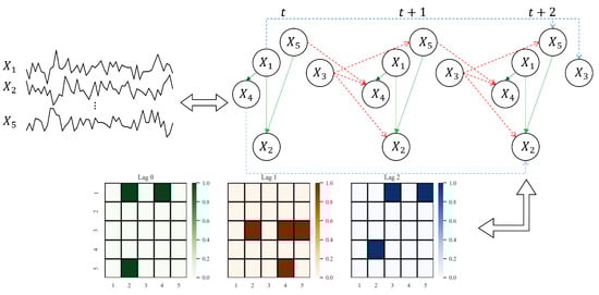
Figure 1. An example showing the correspondence among the given observed variables, the underlying window causal graph, and the window causal matrix. We consider a dataset of $d=5$ observed variables, with a true maximum lag of $\overline{\tau }=2$. In $\mathcal{W}\in {\mathbb{R}}^{5\times 5\times 3}$, for each ${\mathcal{W}}_{i,j}^{\tau }$ represents the causal effect of $X_i$ on $X_j$ with $\tau$ time lags. For example, the blue lines in window causal graph indicate the following three causal effects with time lags $\tau =2$ at any time step t, i.e., ${\mathcal{W}}_{1,3}^2=1\Rightarrow X_1\stackrel{2}{⟶}{X}_3;{\mathcal{W}}_{1,5}^2=1\Rightarrow X_1\stackrel{2}{⟶}{X}_5;{\mathcal{W}}_{4,2}^2=1\Rightarrow X_4\stackrel{2}{⟶}{X}_2$. Moreover, the red lines indicate the causal relationships with time lags $\tau =1$, i.e., ${\mathcal{W}}_{3,2}^1=1\Rightarrow X_3\stackrel{1}{⟶}{X}_2;{\mathcal{W}}_{3,4}^1=1\Rightarrow X_3\stackrel{1}{⟶}{X}_4;{\mathcal{W}}_{3,5}^1=1\Rightarrow X_3\stackrel{1}{⟶}{X}_5;{\mathcal{W}}_{5,4}^1=1\Rightarrow X_5\stackrel{1}{⟶}{X}_4$. Finally, the green lines represent contemporaneous causal relationships, i.e., ${\mathcal{W}}_{1,2}^0=1\Rightarrow X_1\stackrel{0}{⟶}{X}_2;{\mathcal{W}}_{1,4}^0=1\Rightarrow X_1\stackrel{0}{⟶}{X}_4;{\mathcal{W}}_{5,2}^0=1\Rightarrow X_5\stackrel{0}{⟶}{X}_2$.

2.3. Short-Term Causal Invariance

There has been an assertion that causal relationships typically exhibit short-term time and mechanism invariance across extensive time scales [29,30,31]. These two aspects of invariance are commonly regarded as fundamental assumptions of causal invariance in causal discovery from time-series data. In the following, we will present the definitions for these two forms of invariance.

Definition 2 

(Short-Term Time Invariance [29]). Given $\mathcal{X}\in {\mathbb{R}}^{d\times T}$, for any $X_i,X_j,\tau \ge 0$, if $X_i\in P{a}_t^{\tau }\left(X_j\right)$ at time t, then there exists $X_i\in P{a}_{t^{\prime }}^{\tau }\left(X_j\right)$ at time $t^{\prime }\ne t$ in a short period of time, where $P{a}_t^{\tau }(·)$ denotes the set of parents of a variable with τ time lags at time step t.

Short-term time invariance refers to the stability of parent-child causal relationships over time. In other words, it implies that the causal dependencies between variables remain consistent regardless of specific time points. For instance, considering Figure 1: $X_5$ is a parent of $X_4$ with time lag $\tau =1$ at t, then $X_5$ will also be a parent of $X_4$ with time lag $\tau =1$ at $t^{\prime }=t+1$; similarly, when $\tau =0$, if $X_5$ is a parent of $X_2$ at t, then $X_5$ will be a parent of $X_2$ at no matter $t^{\prime }=t+1$ or $t^{\prime }=t+2$.

Definition 3 

(Short-Term Mechanism Invariance [29]). For any $X_i$, the conditional probability distribution $P\left(X_i\right|P{a}_t^{·}\left(X_i\right))$ remains constant across the short-term temporal chain. In other words, for any time step t and $t^{\prime }$, it holds that $P\left(X_i\right|P{a}_t^{·}\left(X_i\right))=P\left(X_i\right|P{a}_{t^{\prime }}^{·}\left(X_i\right))$, where $P{a}_t^{·}\left(X_i\right)$ means the set of parents of $X_i$ with all time lags range from 0 to $\tilde{\tau }$ at time step t.

In particular, based on Definition 3, short-term mechanism invariance implies that conditional probability distributions remain constant over time. For instance, in Figure 1, we have $P{a}_t^{·}\left(X_2\right)=\{X_3,X_1,X_5\}=P{a}_{t+1}^{·}\left(X_2\right)$. Then, we have $P\left(X_2\right|P{a}_t^{·}\left(X_2\right))=P\left(X_2\right|P{a}_{t+1}^{·}\left(X_2\right))$.

Building upon the definitions of short-term time and mechanism invariance, we can derive the following theorem, which characterizes the invariant nature of independence among variables. Inspired by causal invariance [29], we further provide a detailed proof procedure as outlined below.

Theorem 1 

(Independence Property). Given $\mathcal{X}\in {\mathbb{R}}^{d\times T}$ be the observed dataset. If we have $X_i{\underset{t}{\perp \perp }}^{\tau }{X}_j|X_k,...,X_l$, then we have $X_i{\underset{t^{\prime }}{\perp \perp }}^{\tau }{X}_j|X_k,...,X_l$. ${\underset{t}{\perp \perp }}^{\tau }$ means conditional independence with τ time lags at time step t.

Proof. 

Due to the short-term time invariance of the relationships among variables and the short-term mechanism invariance of conditional probabilities, different values $X_i^t$ and $X_i^{t^{\prime }}$ of $X_i$ are mapped to the same variable $X_i$ in the window causal graph $\mathcal{G}$. Consequently, $P{a}_t^{\tau }\left(X_i\right)$ and $P{a}_{t^{\prime }}^{\tau }\left(X_i\right)$ correspond to the same variable set. Thus, if the condition $X_i{\underset{t}{\perp \perp }}^{\tau }{X}_j|X_k,...,X_l$ holds, then $X_i{\underset{\mathcal{G}}{\perp \perp }}^{\tau }{X}_j|X_k,...,X_l$ holds in the window causal graph $\mathcal{G}$, which further implies $X_i{\underset{t^{\prime }}{\perp \perp }}^{\tau }{X}_j|X_k,...,X_l$. □

This theorem establishes that the independence property remains invariant with time translation in an identifiable window causal graph. Leveraging this insight, we can transform the observed time series into window observations to perform causal discovery while maintaining the invariance conditions, as outlined in Section 3.1.

2.4. Necessity of Convolution

Granger demonstrated, through the Cramer representation and the spectral representation of the covariance sequence [20,21,32], that time-series data can be decomposed into a sum of uncorrelated components. Inspired by these representations and the concept of graph Fourier transform [33,34], we propose considering a underlying function $\mathcal{X}=f(P{a}_{\mathcal{G}}\left(\mathcal{X}\right),\mathcal{W})+E$, where $P{a}_{\mathcal{G}}\left(\mathcal{X}\right)$ denotes relationships among $\mathcal{X}$ in the window causal graph $\mathcal{G}$ and E is the noise term, to describe the generative process of the observed dataset $\mathcal{X}=\{X_1,\dots ,X_d\}\in {\mathbb{R}}^{d\times T}$, with an underlying window causal matrix $\mathcal{W}\in {\mathbb{R}}^{d\times d\times (\tilde{\tau }+1)}$. We can then decompose $f(P{a}_{\mathcal{G}}\left(\mathcal{X}\right),\mathcal{W})$ into Fourier integral forms:

$$\begin{array}{cc}\hfill \mathcal{X}& =f(P{a}_{\mathcal{G}}\left(\mathcal{X}\right),\mathcal{W})+E\hfill \\ \hfill & =\widehat{f}(s,t)+E.\hfill \end{array}$$

(1)

Here, s and t denote the spatial and temporal projections, respectively, of $f(P{a}_{\mathcal{G}}\left(\mathcal{X}\right),\mathcal{W})$. Equation (1) is derived from the observation that the contemporaneous part in time-series data corresponds to the spatial domain, while the time-lagged part corresponds to the temporal domain. Therefore, we employ the multivariate Fourier transform,

$$\begin{array}{cc}\hfill \mathcal{F}\left(\mathcal{X}\right)& ={\int \int }_{-\infty }^{\infty }\widehat{f}(x,y;s,t)e^{-i\omega (sx+ty)}dxdy\hfill \\ \hfill & \propto {\int \int }_{-\infty }^{\infty }h\left(\widehat{s}\right)g\left(\widehat{t}\right)e^{-i\omega (\widehat{s}+\widehat{t})}d\widehat{s}d\widehat{t},\hfill \end{array}$$

(2)

where $\widehat{s}$ represents the spatial domain component, $\widehat{t}$ represents the temporal domain component, and $\omega$ represents the angular frequency along with transform function $\widehat{f},h$ and g. The first line corresponds to applying the Fourier transform to both sides of Equation (1). In the second line, inspired by the Time-Independent Schrödinger Equation [35,36], we assume that $f(x,y;s,t)$ can be decomposed into the spatial and temporal domains, i.e., $\widehat{f}(x,y;s,t)=h\left(\widehat{s}\right)g\left(\widehat{t}\right)$. Next, by utilizing the convolution theorem [37] for tempered distributions, which states that under suitable conditions the Fourier transform of a convolution of two functions (or signals) is the pointwise product of their Fourier transform, i.e., $\mathcal{F}(h\ast g)=\mathcal{F}\left(h\right)·\mathcal{F}\left(g\right)$, where $\mathcal{F}(·)$ represents the Fourier transform, we convert the convolution formula into the following expression:

$$\begin{array}{cc}\hfill \mathcal{F}[h\left(\widehat{s}\right)\ast g\left(\widehat{t}\right)]& \propto \mathcal{F}\left(h\left(\widehat{s}\right)\right)·\mathcal{F}\left(g\left(\widehat{t}\right)\right)\hfill \\ \hfill & \propto {\int }_{-\infty }^{\infty }h\left(\widehat{s}\right)e^{-i\omega \widehat{s}}d\widehat{s}{\int }_{-\infty }^{\infty }g\left(\widehat{t}\right)e^{-i\omega \widehat{t}}d\widehat{t}\hfill \\ \hfill & \propto \mathcal{F}\left(\mathcal{X}\right).\hfill \end{array}$$

(3)

The first line of the Formula (3) is obtained through the convolution theorem, while the second line expands $\mathcal{F}\left(h\left(\widehat{s}\right)\right)$ and $\mathcal{F}\left(g\left(\widehat{t}\right)\right)$ using the Fourier transform. The third line is derived from Equation (2). Therefore, it indicates that the observed dataset $\mathcal{X}$ can be obtained by convolving the convolution kernel with temporal information and the spatial details, which we will deal with corresponding to the two kinds of invariance. We posit that the convolution operation precisely aligns with the functional causal data generation mechanism, i.e., $\mathcal{X}\propto h\left(\widehat{s}\right)\ast g\left(\widehat{t}\right)$. Conversely, the convolution operation can be used to analyze the generation mechanism of functional time-series data. Therefore, we will employ the convolution operation to extract the functional causal relationships within the window causal graph. In conclusion, the equivalence between the time-series causal data generation mechanism and convolution operations motivates us to incorporate convolution operations into our STIC framework.

2.5. Granger Causality

Granger causality [20,38] is a method that utilizes numerical calculations to assess causality by measuring fitting loss and variance. In this work, we build on the Granger causality. Granger causality is not necessarily SCM-based since the latter one often considers acyclicity. Under the assumptions of no unobserved variables and no instantaneous effects, ref. [39] shows identifiablility of time-invariant Granger causality [40,41]. Formally, we say that a variable $X_i$ Granger-causes another variable $X_j$ when the past values of $X_i$ at time t (i.e., $X_i^1,\dots ,X_i^{t-1}$) enhance the prediction of $X_j$ at time t (i.e., $X_j^t$) compared to considering only the past values of $X_j$. The definition of Granger causality is as follows:

Definition 4 

(Granger Causality [20]). Let $\mathcal{X}=\{X_1,\dots ,X_d\}\in {\mathbb{R}}^{d\times T}$ be a observed dataset containing d variables. If ${\sigma }_{\tau }^2\left(X_j\right|\mathcal{X})<{\sigma }_{\tau }^2\left(X_j\right|\mathcal{X}-X_i)$, where ${\sigma }_{\tau }^2\left(X_j\right|\mathcal{X})$ denotes the variance of predicting $X_j$ using $\mathcal{X}$ with τ time lags, we say that $X_i$ causes $X_j$, which is represented by ${\mathcal{W}}_{i,j}^{\tau }=1$.

In simpler terms, Granger causality states that $X_i$ Granger-causes $X_j$ if past values of $X_i$ (i.e., $X_i^{t^{\prime }}$) provide unique and statistically significant information for predicting future values of $X_j$ (i.e., $X_j^t$). Therefore, following the definition of Granger causality, we can approach causal discovery as an autoregressive problem.

2.6. Causal Identifiability

As articulated in [12], the identifiability of contemporaneous causality is derived from established results pertaining to vector autoregressive (VAR) models. In contrast, the identifiability of time-lagged causality presents more significant challenges for establishment. We make the following assumptions to ensure causal identification [42]:

• Continuous-valued series: All series are assumed to have continuous-valued observations.
• Stationarity: The statistics of the process are assumed not to change over time.
• Causal Sufficiency: No unmeasured confounders exist.
• Perfectly observed: The variables need to be observed without measurement errors.
• Known lag: The dependency on a history of lagged observations is assumed to have a known order.

Under the above assumptions, this study concentrates on two specific scenarios where identifiability is assured:

• When the errors E are non-Gaussian, identifiability in this model is a well-documented outcome of Marcinkiewicz’s theorem regarding the cumulants of the normal distribution [43,44] and independent component analysis (ICA) [45]. Notably, under faithfulness, (i) if we consider linear functions and non-Gaussian noise, one can identify the underlying directed acyclic graph [46]. (ii) if one restricts the functions to be additive in the noise component and excludes the linear Gaussian case, as well as a few other pathological function-noise combinations, one can show that $\mathcal{G}$ is identifiable [47].
• When the errors E follow a standard Gaussian distribution, specifically $E\sim \mathcal{N}(0,1)$, identifiability in this model arises as a direct consequence of Theorem 1 presented in [48], alongside the acyclicity of $\mathcal{W}$. Specifically, (iii) Gaussian structural equation models where all functions are linear, but the customarily distributed noise variables have equal variances, are again identifiable [48].

In the subsequent discussion, we will assume that one of these two conditions regarding E is satisfied.

3. Methods

In this section, we introduce STIC, which involves four components: Window Representation, Time-Invariance Block, Mechanism-Invariance Block, and Parallel Blocks for Joint Training. The process is depicted in Figure 2. Firstly, we transform the observed time series into a window representation format, leveraging Theorem 1. Next, we input the window representation into both the time-invariance block and the mechanism-invariance block ($B_t$ and $B_m$ in Figure 2). Finally, we conduct joint training using the extracted features from two kinds of parallel blocks. In particular, the time-invariance block $B_t$ generates the estimated window causal matrix $\widehat{\mathcal{W}}$. To better represent the symbols used in Section 3, we also arrange a table to summarize and show their definitions, as shown in Table 2. The subsequent subsections provide a detailed explanation of the key components of STIC.

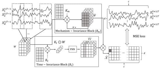
Figure 2. An illustration of the STIC framework. Let $\mathcal{X}=\{X_1,\dots ,X_d\}\in {\mathbb{R}}^{d\times T}$ be the observed dataset, representing d observed continuous time series of the same length T. First, we convert the observations of the first $T-1$ time steps, ${\mathcal{X}}^{1:T-1}=\{X_1^{1:T-1},\dots ,X_d^{1:T-1}\}\in {\mathbb{R}}^{d\times (T-1)}$, into a window representation $W\in {\mathbb{R}}^{d\times \widehat{\tau }\times c}$ using a sliding window with a predefined window length $\widehat{\tau }$ and step length 1, where $c=T-\widehat{\tau }$. Time-Invariance Block ($B_t$): In order to better discover the causal structure from $\mathcal{X}$, we use convolution kernel $K_t\in {\mathbb{R}}^{d\times \widehat{\tau }}$ to act on W, and get the common representation $K_t\odot W_{\psi }$ of $\mathcal{X}$ for each window observations $W_{\psi }$. Afterward, we pass the commonality through an FNN network to obtain a predicted window causal matrix $\widehat{\mathcal{W}}\in {\mathbb{R}}^{d\times d\times \widehat{\tau }}$. Mechanism-Invariance Block ($B_m$): To identify numerical transform in window causal graph, we use another convolution kernel $K_m\in {\mathbb{R}}^{d\times \widehat{\tau }}$ in each $B_m$ to transform W. Then we output $\overline{W}\in {\mathbb{R}}^{d\times \widehat{\tau }\times c}$ as the prediction of $f\left(W\right)$. Next, we do hadamard product of each ${\overline{W}}_{\psi }^{\tau }\in {\mathbb{R}}^d$ in $\overline{W}$ and each ${\widehat{\mathcal{W}}}^{\tau }\in {\mathbb{R}}^{d\times d}$ in $\widehat{\mathcal{W}}$ to get the predicted ${\widehat{\mathcal{X}}}^{\widehat{\tau }+\psi }$ until we get all $\widehat{\mathcal{X}}\in {\mathbb{R}}^{d\times c}$. Finally, we calculate the Mean Squared Error (MSE) loss between $\widehat{\mathcal{X}}$ and $\mathcal{X}$, and adopt gradient descent to optimize the parameters within the time-invariance and mechanism-invariance blocks.

Table 2. Summary of symbol definitions in Section 3.

Symbol	Description
$\overline{\tau }$	The predefined maximum time lag
$\widehat{\tau }$	The predefined window length, $\widehat{\tau }=\overline{\tau }+1$
$W\in {\mathbb{R}}^{d\times \widehat{\tau }\times c}$	The window representation, where $c=T-\widehat{\tau }$
$B_t$	The time-invariance block
$K_t\in {\mathbb{R}}^{d\times \widehat{\tau }}$	The convolution kernel in the time-invariance block
⊙	The Hadamard product
$\widehat{\mathcal{W}}\in {\mathbb{R}}^{d\times d\times (\overline{\tau }+1)}$	The predicted window causal matrix
$B_m$	The mechanism-invariance block
$K_m\in {\mathbb{R}}^{d\times \widehat{\tau }}$	The convolution kernel in the mechanism-invariance block
$\overline{W}\in {\mathbb{R}}^{d\times \widehat{\tau }\times c}$	The prediction of $f\left(W\right)$
$\widehat{\mathcal{X}}\in {\mathbb{R}}^{d\times c}$	The prediction of the observed dataset
$f_1:{\mathbb{R}}^{c\times d\times \widehat{\tau }}\to {\mathbb{R}}^{d\times d\times \widehat{\tau }}$	The feed-forward neural network
${\widehat{\mathcal{W}}}_{i,j}^{\tau }$	The estimated binary existence of the causal effect of $X_i$ on $X_j$ with $\tau$ time lags
p	The threshold used to eliminate edges with low probability of existence
$f_2:{\mathbb{R}}^{d\times \widehat{\tau }}\to {\mathbb{R}}^{d\times \widehat{\tau }}$	The estimated transformation function

To better understand the overall framework of STIC, we need to clarify the following points. First, the input to STIC is $\mathcal{X}=\{X_1,\dots ,X_d\}\in {\mathbb{R}}^{d\times T}$, which is the observed dataset, representing d observed continuous time series of the same length T. The output of STIC is a predicted window causal matrix $\widehat{\mathcal{W}}\in {\mathbb{R}}^{d\times d\times \widehat{\tau }}$ from the Time-Invariance Block. To obtain $\widehat{\mathcal{W}}$, we auto-regress $\mathcal{X}$ as shown in Figure 2, and we combine the Time-Invariance Block and the Mechanism-Invariance Block to train the entire STIC.

3.1. Window Representation

The observed dataset $\mathcal{X}\in {\mathbb{R}}^{d\times T}$ contains d observed continuous time series (variables) with T time steps. We also define a predefined maximum time lag as $\overline{\tau }$. To ensure that the entire causal contemporaneous and time-lagged influence is observed, we calculate the minimum length of the window that can capture this influence as $\widehat{\tau }=\overline{\tau }+1$. To construct the window observations, we select the observed values from the first $T-1$ time steps, i.e., ${\mathcal{X}}^{1:T-1}=\{X_1^{1:T-1},\dots ,X_d^{1:T-1}\}\in {\mathbb{R}}^{d\times (T-1)}$. Using a sliding window approach along the temporal chain of observations, we create window observations of length $\widehat{\tau }$ and width d, with a step size of 1. This process results in $c=T-\widehat{\tau }$ window observations $W_{\psi }$ where $\psi =1,...,c$. These window observations are referred to as the window representation W, as illustrated in Figure 3.

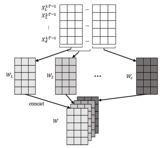
Figure 3. Window representation. First, we get c matrices $W_{\psi }$ by sliding window with predefined window length $\widehat{\tau }$ and step size 1, where each $W_{\psi }\in {\mathbb{R}}^{d\times \widehat{\tau }},\psi =1,...,c$ represents the data we observe in the window. Then, we concatenate the obtained $W_{\psi }$ together to get the final window representation $W\in {\mathbb{R}}^{d\times \widehat{\tau }\times c}$.

3.2. Time-Invariance Block

According to Definition 2, the causal relationships among variables remain unchanged as time progresses. Exploiting this property, we can extract shared information from the window representation W and utilize it to finally obtain the estimated window causal matrix $\widehat{\mathcal{W}}$. Inspired by convolutional neural networks used in causal discovery [13], we introduce an invariance-based convolutional network structure denoted as $B_t$ to incorporate temporal information within the window representation W. For each window observation $W_{\psi }\in {\mathbb{R}}^{d\times \widehat{\tau }}$, we employ the following formula to aggregate similar information among the time series within the window observations,

$$\widehat{\mathcal{W}}=f_1(K_t\odot W_1,...,K_t\odot W_c).$$

(4)

Here, shared $K_t\in {\mathbb{R}}^{d\times \widehat{\tau }}$ represents a learnable extraction kernel utilized to extract information from each window observation. The symbol ⊙ denotes the Hadamard product between matrices, and $f_1$ refers to a neural network structure. By applying the Hadamard product with the shared kernel $K_t$, the resulting output exhibits similar characteristics across the time series. Moreover, $K_t$ serves as a time-invariant feature extractor, capturing recurring patterns that appear in the input series and aiding in forecasting short-term future values of the target variable. In Granger causality, these learned patterns reflect causal relationships between time series, which are essential for causal discovery [49]. To ensure the generality of STIC, we employ a simple feed-forward neural network (FNN) $f_1:{\mathbb{R}}^{c\times d\times \widehat{\tau }}\to {\mathbb{R}}^{d\times d\times \widehat{\tau }}$ to extract shared information from each $K_t\odot W_{\psi },\psi =1,...,c$. Furthermore, we impose a constraint to prohibit self-loops in the estimated window causal matrix $\widehat{\mathcal{W}}$ when the time lag is zero. That is:

$$\begin{array}{c}\hfill {\widehat{\mathcal{W}}}_{i,j}^{\tau }=\left\{\begin{array}{ccc}\hfill 0& & \mathrm{if}i=j\mathrm{and}\tau =0\hfill \\ \hfill 0& & \mathrm{if}{\widehat{\mathcal{W}}}_{i,j}^{\tau }<p\hfill \\ \hfill 1& & \mathrm{else}\hfill \end{array}\right.,\end{array}$$

(5)

where ${\widehat{\mathcal{W}}}_{i,j}^{\tau }$ represents the estimated binary existence of the causal effect of $X_i$ on $X_j$ with a time delay of $\tau \in \{0,...,\overline{\tau }\}$, and p is a threshold used to eliminate edges with low probability of existence.

3.3. Mechanism-Invariance Block

As stated in Definition 3, the causal conditional probability relationships among the time series remain unchanged as time varies. Consequently, the causal functions between variables also remain constant over time. With this in mind, our objective in $B_m$ is to find a unified transform function $f_2:{\mathbb{R}}^{d\times \widehat{\tau }}\to {\mathbb{R}}^{d\times \widehat{\tau }}$ that accommodates all window observations. To achieve this goal, as depicted in Figure 2, we employ a convolution kernel $K_m\in {\mathbb{R}}^{d\times \widehat{\tau }}$ as $f_2$. This kernel performs a Hadamard product operation with each window $W_{\psi }\in {\mathbb{R}}^{d\times \widehat{\tau }}$ in W, where $\psi =1,...,c$. Subsequently, we employ the Parametric Rectified Linear Unit (PReLU) activation function [50] to obtain the output ${\overline{W}}_{\psi }\in {\mathbb{R}}^{d\times \widehat{\tau }}$,

$${\overline{W}}_{\psi }=PReLU(K_m\odot W_{\psi }).$$

(6)

Each ${\overline{W}}_{\psi }$ represents the transformed matrix obtained from the window observation $W_{\psi }$ by a unified transform function $f_2$ implemented with convolution kernel $K_m$. Each ${\overline{W}}_{\psi }$ is finally used to predict ${\widehat{\mathcal{X}}}^{\widehat{\tau }+\psi }$. Note that this transform function $f_2$ can also be composed of N different but equal dimensional kernels $K_m^1,...,K_m^N\in {\mathbb{R}}^{d\times \widehat{\tau }}$, which are nested to perform complex nonlinear transformations. After $f_2$, the value inside the window $W_{\psi }\in {\mathbb{R}}^{d\times \widehat{\tau }}$ is then pressed for $\widehat{\mathcal{W}}$-selected column summation to predict ${\widehat{\mathcal{X}}}^{\widehat{\tau }+\psi }\in {\mathbb{R}}^d$.

3.4. Parallel Blocks for Joint Training

So far, we have obtained the estimated window causal matrix $\widehat{\mathcal{W}}$ by using $B_t$. In addition, we also obtained the transformed matrix $\overline{W}$ with $B_m$. We used convolutional neural networks in both $B_t$ and $B_m$. Their structures are similar, but their functions and purposes are different. In $B_t$, we focus on the shared underlying unified structure of all window observations. Following the Definition 2 of short-term time invariance, we choose a convolutional neural network structure with translation invariance [51,52]. We expect that $f_1$ with $K_t$ as the main component can extract the invariant structure of the window representation W. In $B_m$, we focus on the convolution kernel $K_m$, which is expected to serve as a unified transform function $f_2$ to satisfy the Definition 3 of short-term mechanism invariance and perform complex nonlinear transformations.

Based on Definition 4 described in Section 2.5, after obtaining the estimated window causal matrix and the transform functions between variables, we can combine the outputs from the time-invariance and mechanism-invariance blocks and using $\widehat{\mathcal{W}}$-selected column summation to predict $\widehat{\mathcal{X}}$. We consider that the time-invariance block facilitates the identification of parent-child relationships between variables, formalized as $\widehat{\mathcal{W}}$, while the mechanism-invariance block helps to explore the generative mechanisms, i.e., transform functions. Consequently, we can naturally combine the outputs $\widehat{\mathcal{W}}$ and $\overline{W}$. Specifically, by utilizing $\widehat{\mathcal{W}}$ and the computed ${\overline{W}}_{\psi },\psi =1,...,c$, we can ultimately obtain the estimates ${\widehat{\mathcal{X}}}^{\widehat{\tau }+\psi }$, namely $\widehat{\mathcal{W}}$-selected column summation,

$${\widehat{\mathcal{X}}}^{\widehat{\tau }+\psi }=\sum _{\tau =0}^{\overline{\tau }}{\overline{W}}_{\psi }^{\tau }\odot {\widehat{\mathcal{W}}}^{\tau }.$$

(7)

Here, we need to consider each $\tau \in \{0,...,\overline{\tau }\}$ and combine the estimated window causal matrix $\widehat{\mathcal{W}}$ with the corresponding transformed window observations ${\overline{W}}_{\psi }$ obtained through $B_m$ to obtain the values of ${\widehat{\mathcal{X}}}^{\widehat{\tau }+\psi }$. Our ultimate goal is to find a window causal matrix $\widehat{\mathcal{W}}$ that satisfies the conditions by optimizing the mean squared error loss (MSE) $\mathcal{L}$ between the predicted $\widehat{\mathcal{X}}$ and the ground truth $\mathcal{X}$ at each time point t. The final auto-regressive equation is expressed as follows:

$$\mathcal{L}=\sum _{t=\widehat{\tau }+1}^T\sum _{i=1}^d\left|\right|X_i^t-{\widehat{\mathcal{X}}}_i^t{\left|\right|}_2^2.$$

(8)

We adopt the gradient $▽\mathcal{L}$ to optimize the parameters within the time-invariance and mechanism-invariance blocks.

4. Results

In this section, we present a comprehensive series of experiments on both synthetic and benchmark datasets to verify the effectiveness of the proposed STIC. Following the experimental setup of [8,9], we compare STIC against the constraint-based approaches such as PCMCI [8], PCMCI+ [9] and ARROW [10], the score-based approaches such as VARLINGAM [11], DYNOTEARS [12], and the Granger-based approaches TCDF [13], CUTS [14] and CUTS+ [15].

Our causal discovery algorithm is implemented using PyTorch 2.4.0+cu121. The source code for our algorithm is publicly available at the following https://github.com/HITshenrj/STIC (accessed on 7 November 2025). Both the time-invariance block and mechanism-invariance block are implemented using convolutional neural networks. Firstly, we conducted experiments on synthetic datasets, encompassing both linear and non-linear cases. The methods of generating synthetic datasets for both linear and nonlinear cases will be introduced separately in Section 4.2. Secondly, we proceeded to perform experiments on benchmark datasets to demonstrate the practical value of our model in Section 4.3. Thirdly, to evaluate the sensitivity of hyper-parameters, such as the learning rate (default 1 × ${10}^{-5}$), the predefined $\overline{\tau }$ (default $0.4d$) and the threshold p (default $0.3$), we conducted ablation experiments as detailed in Section 4.4. We trained STIC with the same epoch number as other gradient-based baselines, such as DYNOTEARS [12], TCDF [13], CUTS [14], and CUTS+ [15]. This maintains the same time complexity among all gradient-based methods.

We employ two kinds of evaluation metrics to assess the quality of the estimated causal matrix: the F1 score and precision. A higher F1 score indicates a more comprehensive estimation of the window causal matrix, while a higher precision indicates the ability to identify a larger number of causal edges. In this paper, we consider causal edges with different time lags for the same pair of variables as distinct causal edges. Specifically, if there exists a causal edge from $X_i$ to $X_j$ with a time lag of ${\tau }_1$, and another causal edge from $X_i$ to $X_j$ with the time lags of ${\tau }_2$, where $i\ne j$ and ${\tau }_1\ne {\tau }_2$, we regard these as two separate causal edges. Due to the need to predefine the maximum time lag in STIC, we truncate the estimated $\widehat{\mathcal{W}}\in {\mathbb{R}}^{d\times d\times (\overline{\tau }+1)}$ to $\mathcal{W}\in {\mathbb{R}}^{d\times d\times (\tilde{\tau }+1)}$ and then compute the evaluation metrics. We handle other baselines (such as VARLINGAM, PCMCI, PCMCI+, DYNOTEARS, CUTS, CUTS+ and ARROW) requiring a predefined maximum time lag parameter in the same manner.

Specifically, assuming the predicted window causal matrix is $\widehat{\mathcal{W}}\in {\mathbb{R}}^{d\times d\times \widehat{\tau }}$, and the ground truth window causal matrix is $\mathcal{W}\in {\mathbb{R}}^{d\times d\times \widehat{\tau }}$, we calculate the F1 score and precision using Equations (9) and (10) with $1(·)$ an indicator function.

$$\mathrm{Precision}={\displaystyle \frac{{\sum }_{i,j,\tau }1({\widehat{\mathcal{W}}}_{i,j}^{\tau }\ne 0\wedge {\mathcal{W}}_{i,j}^{\tau }\ne 0)}{{\sum }_{i,j,\tau }1({\widehat{\mathcal{W}}}_{i,j}^{\tau }\ne 0)}}.$$

(9)

$$\mathrm{F}1=2·{\displaystyle \frac{\mathrm{Precision}\times \mathrm{Recall}}{\mathrm{Precision}+\mathrm{Recall}}},\mathrm{where}\mathrm{Recall}={\displaystyle \frac{{\sum }_{i,j,\tau }1({\widehat{\mathcal{W}}}_{i,j}^{\tau }\ne 0\wedge {\mathcal{W}}_{i,j}^{\tau })}{{\sum }_{i,j,\tau }1({\mathcal{W}}_{i,j}^{\tau }\ne 0)}}.$$

(10)

4.1. Baselines

We select eight state-of-the-art causal discovery methods as baselines for comparison:

• VARLINGAM [11] shows how to combine the non-Gaussian instantaneous model with autoregressive models. Such a non-Gaussian model has been proven to be identifiable without prior knowledge of the network structure. In VARLINGAM, computationally efficient methods are proposed for estimating the model, as well as methods to assess the significance of the causal influences. The source code for VARLINGAM is available at https://lingam.readthedocs.io/en/latest/tutorial/var.html (accessed on 7 November 2025).
• PCMCI [8] is a notable work that extends the PC algorithm [53] for causal discovery from time-series data. The source code for PCMCI is available at https://github.com/jakobrunge/tigramite (accessed on 7 November 2025). PCMCI divides the causal discovery process into two components: the identification of relevant sets through conditional independence tests and the direction determination. It assumes causal stationarity, the absence of contemporaneous causal links, and no hidden variables. Specifically, the PC-stable algorithm [54] is employed to remove irrelevant conditions through iterative independence tests. Furthermore, the Multivariate Conditional Independence test addresses false-positive control in highly interdependent time series scenarios.
• PCMCI+ [9] improves upon PCMCI by reducing the number of independence tests and optimizing the selection of conditional sets, resulting in superior effectiveness and efficiency in the same experimental setting. The source code is also available at https://github.com/jakobrunge/tigramite (accessed on 7 November 2025). PCMCI+ overcomes the limitation of the “no contemporaneous causal links” assumption in PCMCI. PCMCI+ expedites the selection of conditional sets by testing all time-lagged pairs conditional on only the strongest p adjacencies in each p-iteration without evaluating all p-dimensional subsets of adjacencies. Moreover, intra-slice sets are introduced to refine the determination of all structures further.
• DYNOTEARS [12] represents a groundbreaking advancement in the field of causal discovery from time-series data by transforming the combinatorial graph search problem into a continuous optimization problem. The details of this work can be found in the repository located at https://github.com/ckassaad/causal_discovery_for_time_series (accessed on 7 November 2025). This approach characterizes the acyclicity constraint as a smooth equality constraint through the minimization of a penalized loss while adhering to the acyclicity constraint.
• TCDF [13] is an outstanding work that utilizes attention-based convolutional neural networks (CNNs) to explore causal relationships between time series and the time delay between cause and effect. The code for TCDF can be accessed at https://github.com/M-Nauta/TCDF (accessed on 7 November 2025). By leveraging Granger causality, TCDF predicts one time series based on other time series and its own historical values, employing CNNs to identify and analyze causal relationships within time-series data.
• CUTS [14] is an outstanding neural Granger causal discovery algorithm for jointly imputing unobserved data points and building causal graphs by incorporating two mutually boosting modules (latent data prediction and causal graph fitting) in an iterative framework. After hallucinating and registering unstructured data, which might be of high dimension and have complex distribution, CUTS builds a causal adjacency matrix with imputed data under a sparse penalty. The code for CUTS is available at https://github.com/jarrycyx/UNN/tree/main/CUTS (accessed on 7 November 2025). CUTS is a promising step toward applying causal discovery to real-world applications with non-ideal observations.
• CUTS+ [15] is built on the Granger-causality-based causal discovery method CUTS and increases scalability through coarse-to-fine discovery and message-passing-based methods. The code for CUTS+ can be accessed at https://github.com/jarrycyx/UNN/tree/main/CUTS_Plus (accessed on 7 November 2025). CUTS+ significantly improves causal discovery performance on high-dimensional data with various types of irregular sampling.
• ARROW [10] is a causal discovery accelerator that incorporates time weaving to efficiently encode time series data to capture the dynamic trends. Following that, XOR operations are used to obtain the optimal time lag. Last, to optimize the search space for causal relationships, a pruning strategy is designed to identify the most relevant candidate variables, enhancing the efficiency and accuracy of causal discovery. The code for ARROW is available at https://github.com/XiangguanMu/arrow (accessed on 7 November 2025). In our experiments, we implement ARROW based on VARLINGAM.

4.2. Results on Synthetic Datasets

We generate synthetic datasets in the following manner. Firstly, following an additive noise model, we consider several typical challenges [8,9] with contemporaneous and time-lagged causal dependencies. We set the ground truth maximum time lag to $0.4d$ and initialize the existence of each edge in the true window causal matrix $\mathcal{W}$ with a probability of 50%. For each variable $X_i$, its relation to with its parents $P{a}_{\mathcal{G}}\left(X_i\right)$ is defined as $X_i=f_i\left(P{a}_{\mathcal{G}}\left(X_i\right)\right)+{\epsilon }_i$, where $f_i$ represents the ground truth transformation function between $X_i$’s parents $P{a}_{\mathcal{G}}\left(X_i\right)$ and $X_i$. If $X_j\in P{a}_{\mathcal{G}}^{\tau }\left(X_i\right)$, then in the ground truth causal matrix $\mathcal{W}$, ${\mathcal{W}}_{ji}^{\tau }=1$. Secondly, for linear datasets, each $f_i$ is defined by a weighted linear function, while for nonlinear datasets, each $f_i$ is defined using a weighted cosine function. We sample the weights from a uniform distribution. If a causal edge exists, the corresponding weight in the additive noise model is sampled from the interval $U(-2,-0.5]\cup [0.5,2)$ to ensure non-zero values. For non-causal edges, the weight is set to 0. The noise term ${\epsilon }_i$ follows either a standard normal distribution $\mathcal{N}(0,1)$ or is uniformly sampled from the interval $U[0,1]$. These data-generating procedures are similar to those used by the PCMCI family [8,9] and CUTS family [14,15].

In the following, we present different results on linear Gaussian datasets (Section 4.2.1), nonlinear Gaussian datasets (Section 4.2.2), and linear uniform datasets (Section 4.2.3) to demonstrate the superiority of our model. Specifically, to reduce the impact of random initialization, we conduct 10 experiments for each type of dataset and report the experimental results.

4.2.1. Results on Linear Gaussian Datasets

The data generation process for linear Gaussian datasets follows the relationship $X_i=w_{i}P{a}_{\mathcal{G}}\left(X_i\right)+{\epsilon }_i$, where ${\epsilon }_i$ is sampled from a standard normal distribution $\mathcal{N}(0,1)$. To demonstrate the capability of our model in causal discovery from time-series data on datasets of varying sizes, we compare STIC with baselines under different conditions, including different numbers of variables ($d=\{5,10,15,20\}$) and different lengths of time steps ($T=\{100,200,500,1000\}$).

The results are summarized in Figure 4. Figure 4 left presents the variation of the F1 score as the number of variables increases, while Figure 4 right shows the variation of precision with the number of variables. A comprehensive analysis of the experiments requires the joint consideration of both Figure 4 left and right. From a macroscopic perspective, our proposed STIC achieves the highest F1 scores on linear Gaussian datasets, while precision reaches the state-of-the-art levels in most cases. We will compare the performance of STIC and the baselines from two aspects of analysis:

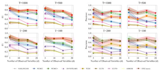
Figure 4. The results of F1 (detailed in Figure 4 (left)) and precision (detailed in Figure 4 (right)) evaluated on linear Gaussian datasets with varying numbers of variables (d) and observed time steps (T). The observed data $\mathcal{X}$ is generated by sampling d time series with T observed time steps from a linear Gaussian distribution. We consider different values of d ranging from 5 to 20 and varying observed time steps T, including 100, 200, 500, and 1000. We report the mean and standard deviation of experimental results.

Aspect 1: The relationship between the number of variables d and the model when T remains constant. When the observed time steps are fixed at $T=1000$, corresponding to the top-left graphs in Figure 4 left and right, we observe that as the number of variables increases, the F1 scores of all causal discovery methods tend to decrease. However, our proposed STIC achieves an average F1 score of 0.86, 0.77, 0.79, and 0.77, as well as an average precision of 0.80, 0.62, 0.74, and 0.72 across the four different numbers of variables, surpassing other strong baselines. By comparing the line plots in the corresponding positions of Figure 4 left and right, especially when $T=100$, corresponding to the bottom-right graphs in Figure 4 left and right, we find that our proposed STIC achieves an average F1 score of 0.76, 0.76, 0.77, 0.65 and an average precision of 0.66, 0.70, 0.77, 0.65 across the four different numbers of variables, significantly outperforming other strong baselines.

In the case of fixed observed time steps, as the number of variables increases, constraint-based approaches such as PCMCI and PCMCI+ suffer from severe performance degradation because they require significant prior knowledge to determine the threshold p, which determines the presence of causal edges. For score-based methods, the DYNOTEARS method exhibits relatively stable performance as the number of variables increases; however, it does not achieve the optimal performance among all methods. VARLINGAM, based on non-Gaussian instantaneous, cannot successfully complete the causal discovery task. Although ARROW utilizes time weaving to better capture dynamic trends, it suffers from the limitations of its base causal discovery model, resulting in a lack of improvement in F1 and precision. As for Granger-based methods, CUTS and CUTS+ often suffer from poor performance due to the inability to recognize time lags. Our proposed STIC and the TCDF method achieve competitive results in terms of F1 scores. However, our method exhibits higher precision.

We attribute this superior performance to the window representation employed in STIC. By repeatedly extracting features from observed time series in different window observations, such a representation acts as a form of data augmentation and aggregation. It enables a macroscopic view of common characteristics among multiple window observations, facilitating the learning of more accurate causal structures. Thus, our STIC model achieves optimal performance when the number of variables d changes.

Aspect 2: The relationship between the observed time steps T and the model when d remains constant. When examining the impact of observed time steps T on the models while keeping the number of variables constant, we observe that our STIC method consistently maintains an F1 score of approximately 0.7 across different values of T. However, PCMCI+ and DYNOTEARS exhibit a significant decline in their F1 scores as T decreases. For instance, at $T=1000$, PCMCI+ and DYNOTEARS perform similarly to our STIC method, but at $T=100$, their F1 scores drop to half of that achieved by our STIC method. For PCMCI, it consistently falls behind our STIC method, regardless of changes in T. While TCDF achieves a relatively consistent level of performance, it exhibits lower performance compared to our model. Furthermore, we find that after treating different time lags as distinct causal edges, the F1 scores and precisions of VARLINGAM, CUTS, CUTS+, and ARROW remain at a relatively low level.

For constraint-based approaches, PCMCI and PCMCI+ algorithms perform poorly because, as the number of samples decreases, the statistical significance of conditional independence cannot fully capture the causal relationships between variables. As for score-based methods, DYNOTEARS does not perform well on linear data. One possible reason is that DYNOTEARS heavily relies on acyclicity in its search, which may not converge to the correct causal graph. One reason why VARLINGAM and ARROW do not perform well is mainly due to the strong assumptions about data distribution. Regarding Granger-based methods, we believe that they are overly conservative and fail to accurately predict all correct causal edges.

In contrast, our STIC model is capable of predicting a greater number of causal edges, which is crucial for discovering new knowledge. This superior performance can be attributed to the design of the convolutional time-invariance block. This design enables the extraction of more causal structure features from limited observed data, allowing for a more accurate exploration of potential causal relationships, even with a small number of samples. Consequently, our STIC model effectively addresses the challenge of causal discovery in low-sample scenarios, i.e., improving sample efficiency.

4.2.2. Results on Nonlinear Gaussian Datasets

In this section, we perform experiments on nonlinear Gaussian datasets to evaluate the performance of STIC. We set the number of variables $(d=5)$ and the observed time steps $(T=1000)$. For each $X_i$, its relationship with its parents $P{a}_{\mathcal{G}}\left(X_i\right)$ is defined using the cosine function, and the noise term ${\epsilon }_i$ follows the standard normal distribution.

The performance of STIC and the baselines is visualized in Figure 5. It can be observed that STIC achieves a median F1 score of 0.44, which is higher than all baselines (VARLINGAM: 0.23, PCMCI: 0.41, PCMCI+: 0.43, DYNOTEARS: 0.22, TCDF: 0.43, CUTS: 0.24, CUTS+: 0.37, ARROW: 0.23). It can be seen that STIC achieves a higher F1 score despite having lower precision compared to the other baselines. For constraint-based methods (PCMCI and PCMCI+), one possible reason for achieving similar F1 scores with our proposed STIC is that the length of observed time steps is set to 1000, which is sufficient for statistical independence tests. Thus, the conditional independence tests can directly operate on the data without being affected by noise. Regarding score-based methods, we believe that VARLINGAM, DYNOTEARS, and ARROW employ a simple network that may not effectively capture nonlinear transformations, resulting in lower F1 scores. For Granger-based methods, although TCDF achieves a comparable F1 score to STIC (and even higher precision), the interquartile range of STIC is significantly lower. This suggests that TCDF is highly unstable, and there is considerable uncertainty in the causal discovery process. One possible reason for this is that TCDF does not incorporate window representation like STIC, which could lead to inefficient training of the convolutional neural network. We find that CUTS and CUTS+ are not very effective at causal discovery on nonlinear Gaussian datasets, and both $F1$ and precision scores are lower than those of our STIC. One possible reason is that both models rely on graph neural networks and treat learnable graph structures as estimated causal graphs. However, the graph structure in the graph neural network is full of correlational relationships rather than causal relationships, so the output graph structure does not contain only causal relationships, resulting in a decrease in both F1 and precision. We believe that the robustness of our proposed STIC lies in the mechanism-invariance block, which repeatedly verifies the functional causal relationships within each single window, effectively reducing model instability.

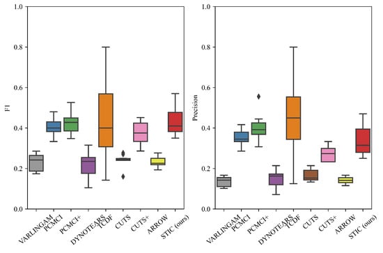
Figure 5. The results of F1 and precision evaluated on nonlinear Gaussian datasets. We fix the numbers of variables $d=5$ and observed time steps $T=1000$. We report the median and quartiles of experimental results. The diamond symbol represents outliers in a box plot that significantly differ from other values.

4.2.3. Results on Linear Uniform Datasets

The linear uniform datasets are generated with observed time steps ($T=1000$) by varying numbers of variables ($d=\{5,10,15,20\}$). For each $X_i$, $f_i$ is set as a linear function, while the noise term ${\epsilon }_i$ follows a uniform distribution $U[0,1]$.

The performance of STIC and baselines is shown in Figure 6. STIC outperforms baselines in terms of F1 score and precision in most cases, especially when the number of time series d is large. For constraint-based methods, PCMCI and PCMCI+ perform poorly in terms of F1 score and precision when the number of variables is relatively large ($d=\{10,15,20\}$). We consider that since conditional independence tests serve as strict indicators of causal relationships, they may fail due to the limited number of time steps and the presence of uniform noise. Moreover, PCMCI cannot determine intra-slice causal relationships and performs much worse than our STIC model in terms of F1 score and precision. For score-based methods, VARLINGAM, DYNOTEARS, and ARROW identify causal relationships by fitting auto-regressive coefficients between variables, treating them as estimated causal relationships. However, due to the strong influence of noise, they fail to recognise causal relationships in the linear uniform datasets. Interestingly, TCDF, which shows competitive performance compared to our STIC model in Section 4.2.1, performs particularly poorly on the linear uniform datasets. From the high precision and low F1 score of TCDF, we can deduce that the uniform distribution introduces many incorrectly estimated causal edges during the process of estimating temporal causality based on Granger causality using the past value of other variables. The F1 score and precision of CUTS and CUTS+ further support the idea that Granger causality is not well applicable to linear uniform datasets. One possible reason is that for a uniform distribution, its inverse transformation equation still exists, which leads to the performance degradation of finding causality from correlation.

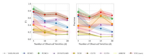
Figure 6. The results of F1 and precision evaluated on linear uniform datasets with fixed observed time steps ($T=1000$) and the number of variables (d) ranging from 5 to 20. We report the mean and standard deviation of experimental results.

4.3. Results on fMRI Benchmark Dataset

In this section, we utilize fMRI benchmark datasets, a common neuroscientific benchmark dataset called Functional Magnetic Resonance Imaging [55], to explore and discover brain blood flow patterns. The dataset comprises 28 distinct underlying brain networks, each with a varying number of observed variables ($d=\{5,10,15\}$). For each of the 28 brain networks, we observe 200 time steps for causal discovery. The results are reported in Table 3.

Table 3. The results of F1 and precision evaluated on the fMRI dataset. Regarding the average of both F1 and precision, STIC outperforms the other baselines. We report the mean and standard deviation of experimental results.

		VARLINGAM	PCMCI	PCMCI+	DYNOTEARS	TCDF	CUTS	CUTS+	ARROW	STIC (Ours)
$d=5$	F1	0.51 ± 0.042	0.38 ± 0.061	0.37 ± 0.095	0.43 ± 0.097	0.42 ± 0.081	0.35 ± 0.031	0.36 ± 0.184	0.50 ± 0.043	0.45 ± 0.029
	precision	0.35 ± 0.040	0.31 ± 0.118	0.33 ± 0.126	0.31 ± 0.131	0.44 ± 0.080	0.22 ± 0.082	0.29 ± 0.187	0.34 ± 0.039	0.70 ± 0.189
$d=10$	F1	0.31 ± 0.030	0.24 ± 0.035	0.31 ± 0.030	0.20 ± 0.049	0.42 ± 0.033	0.11 ± 0.036	0.44 ± 0.032	0.30 ± 0.089	0.47 ± 0.039
	precision	0.18 ± 0.074	0.34 ± 0.029	0.37 ± 0.027	0.33 ± 0.060	0.44 ± 0.057	0.20 ± 0.020	0.51 ± 0.034	0.18 ± 0.080	0.60 ± 0.094
$d=15$	F1	0.23 ± 0.050	0.27 ± 0.054	0.35 ± 0.084	0.19 ± 0.110	0.35 ± 0.047	0.14 ± 0.028	0.26 ± 0.142	0.23 ± 0.085	0.53 ± 0.075
	precision	0.13 ± 0.044	0.19 ± 0.043	0.20 ± 0.024	0.11 ± 0.102	0.43 ± 0.179	0.08 ± 0.040	0.26 ± 0.055	0.13 ± 0.077	0.80 ± 0.068

The results demonstrate that STIC achieves the highest average F1 scores on most observed variables, surpassing the average F1 scores of VARLINGAM, PCMCI, PCMCI+, DYNOTEARS, TCDF, CUTS, CUTS+, and ARROW. Moreover, in terms of precision, STIC achieves significantly higher precision than all other baselines. For constraint-based methods, such as PCMCI and PCMCI+, their poor performance on the fMRI datasets may be attributed to the short length of observed time steps, which affects their ability to accurately test for conditional independence. Regarding DYNOTEARS, we believe that acyclicity regularizers still limit its performance. As for VARLINGAM and ARROW, the performance reduction is mainly due to the conflict between the data distribution assumption and the real world. In comparison, our STIC model outperforms TCDF, CUTS, and CUTS+ by utilizing a window representation, which enhances the representation of observed data within each window. This enables more accurate learning of common causal features and structures across multiple windows.

Comparing the standard deviation of STIC’s F1 score under various numbers of variables, results show that it maintains a low level ($d=5$: 0.029, $d=10$: 0.039, and $d=15$: 0.075). While CUTS achieves a similar standard deviation with STIC at $d=5$, its mean F1 score is significantly lower than that of STIC. At $d=15$, although many baselines achieve lower standard deviation, even down to 0.050, one possible reason is that their F1 scores are also low, resulting in minimal variability across different data points. STIC’s F1 score can even reach twice that of the baseline in some cases, while its standard deviation remains on the same order of magnitude, demonstrating its stability.

4.4. Ablation Study

We conduct ablation experiments on the linear Gaussian datasets with the number of variables ($d=5$) to investigate the impact of different hyper-parameters on the experimental results, such as the learning rate (default: 1 × ${10}^{-5}$), the predefined maximum time lag (default: $0.4d=2$), and the threshold p (default: 0.3). Specifically, we vary the learning rate by increasing it to 1 × ${10}^{-4}$ and decreasing it to 1 × ${10}^{-6}$. We also increased the predefined maximum lag to $\overline{\tau }=3$ and $\overline{\tau }=4$, respectively, and changed the threshold to $p=0.1$ or $p=0.5$. The empirical results are summarized in Table 4.

Table 4. The results of the ablation study on the linear Gaussian datasets with the number of variables ($d=5$).

Hyper-Parameters	Value	F1	Precision
Learning Rate	lr = 1 × ${10}^{-4}$	0.77 ± 0.005	0.66 ± 0.006
	lr = 1 × ${10}^{-5}$	0.76 ± 0.008	0.66 ± 0.013
	lr = 1 × ${10}^{-6}$	0.78 ± 0.004	0.68 ± 0.016
Max Time Lag	$\overline{\tau }=2$	0.76 ± 0.008	0.66 ± 0.013
	$\overline{\tau }=3$	0.68 ± 0.004	0.53 ± 0.005
	$\overline{\tau }=4$	0.60 ± 0.003	0.45 ± 0.003
Threshold	$p=0.1$	0.43 ± 0.001	0.27 ± 0.001
	$p=0.3$	0.76 ± 0.008	0.66 ± 0.013
	$p=0.5$	0.80 ± 0.020	0.89 ± 0.019

• The learning rate lr: The experiments reveal that manipulating the learning rate, either by increasing or decreasing it, has little effect on the F1 score and precision. This finding suggests that our convolutional neural network architecture is not sensitive to changes in the learning rate, simplifying the parameter tuning process.
• The predefined maximum time lag $\overline{\tau }$: However, increasing the predefined maximum lag $\overline{\tau }$ gradually deteriorates performance. We speculate that this decline occurs because, with a longer lag, the window for observations expands, potentially causing STIC to learn multi-hop causal edges ($X_i\stackrel{{\tau }_1}{⟶}{X}_j\stackrel{{\tau }_2}{⟶}{X}_k$) as single-hop causal edges ($X_i\stackrel{{\tau }_1+{\tau }_2}{⟶}{X}_k$). Addressing this issue could be a focus for future research.
• The threshold p: Furthermore, comparing the default setting to STIC with $p=0.1$, we observe a significant decline in both F1 score and precision when the threshold is lower. When comparing the default setting to STIC with $p=0.5$, we find that while the F1 score remains relatively stable, precision notably improves when the threshold is increased. These findings indicate that reducing the threshold adversely affects the model’s ability to explore causal edges, while setting a higher threshold may cause the model to consider nearly all estimated edges as causal, resulting in increased precision but a similar F1 score. Thus, the threshold plays a pivotal role in discovering more causal edges, and a trade-off needs to be made.

4.5. Visualization

In this section, we present the causal discovery visualization results for STIC under three types of datasets: linear Gaussian datasets (Figure 7), nonlinear Gaussian datasets (Figure 8), and linear uniform datasets (Figure 9). To avoid redundancy, we display results for $d=5$ under conditions of $T=1000$. The visualization aims to specify which specific patterns STIC captures and serves as a measure of the interpretability of our model.

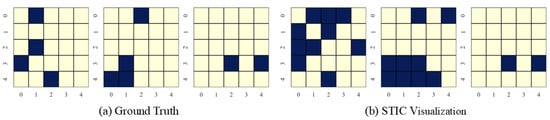
Figure 7. Visualization of experimental results on linear Gaussian datasets with the number of variables $d=5$ and observed time steps $T=1000$.

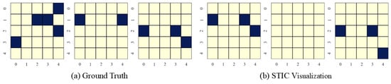
Figure 8. Visualization of experimental results on nonlinear Gaussian datasets with the number of variables $d=5$ and observed time steps $T=1000$.

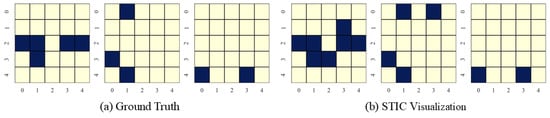
Figure 9. Visualization of experimental results on linear uniform datasets with the number of variables $d=5$ and observed time steps $T=1000$.

STIC is built on the premise that if a model can accurately predict the world, it must have learned the causal structure of the world [56,57]. The visualization results show that the time-invariance block of STIC identifies almost all true causal edges, although it may also detect a small number of spurious edges. Using the edges inferred by the time-invariance block, STIC then applies an autoregressive mechanism to compute the MSE loss between the predicted and observed time series. The interpretability of STIC is primarily reflected in the time-invariance block, as it explicitly discovers the causal graph and uses that graph as the foundation for prediction, thereby ensuring the interpretability of the entire framework.

5. Discussion

This study presents two short-term invariance-based convolutional neural networks for discovering causality from time-series data. Major findings include: (1) Our methods, based on gradients, effectively discover causality from time-series data; (2) Convolutional neural networks based on short-term invariance improve the sample efficiency of causal discovery. (3) Our proposed STIC performs significantly better than baseline causal discovery algorithms. In this section, we discuss these results in detail.

5.1. What Contributes to the Effectiveness of STIC?

5.1.1. Why Can STIC Find Causal Relationships?

Numerous gradient-based methods have been developed, such as score-based approaches (DYNOTEARS) [12], and TCDF [13], CUTS [14], and CUTS+ [15] within Granger-based approaches. Including our proposed STIC, these gradient-based methods aim to optimize the estimated causal matrix by maximizing or minimizing constrained functions. With the rapid advancement and widespread adoption of deep Neural Networks (NNs), researchers have begun employing NNs to infer nonlinear Granger causality, demonstrating the effectiveness of gradient-based methods in causal discovery [58,59,60]. In our approach, we maintain the assumptions and constrained functions of Granger causality, ensuring that our method remains effective in discovering causal relationships.

5.1.2. Why Can STIC Find the True Causality?

As time progresses, the values of observed variables change due to shifts in the statistical distribution. However, the causal relationships between the variables remain the same. For example, carbohydrate intake may lead to an increase in blood glucose, but the specific magnitude of this increase may vary depending on covariates such as body weight. The “lead” property indicates causal relationships, i.e., invariance [61,62,63,64]. In this paper, we observe that some causal relationships may also vary over time. Therefore, we make a more reasonable assumption: short-term time invariance and mechanism invariance [29,30,31]. Building on these two forms of short-term invariance, we posit that both the window causal matrix $\mathcal{W}$ and the transform function f remain unchanged in the short term. For example, within a short term (a few days), since covariates affecting blood glucose levels, such as body weight, remain nearly constant, the increase in blood glucose levels due to carbohydrate intake is also essentially constant. The short-term mechanism invariance proposed in this paper is also considered an invariant principle [65]. Building on these forms of invariance, a natural extension is the introduction of parallel time-invariance and mechanism-invariance blocks for joint training, as proposed in this paper. Through the theoretical validation of convolution in Section 2.4, we further affirm the applicability of convolution to causal discovery from time-series data. Additionally, the Granger causality is commonly employed to examine short-term causal relationships [66], further aligning with our assumptions. Under the premise of theoretical soundness and practical applicability, our STIC framework proves highly effective.

5.2. What Contributes to the Exceptional Performance of STIC?

5.2.1. High F1 Scores and Precisions

The experiments conducted on both synthetic and fMRI datasets in Section 4 demonstrate that our STIC model achieves the state-of-the-art F1 scores and precisions in most cases. We attribute the performance improvement to the incorporation of the window representation, the time-invariance block, and the mechanism-invariance block. The window representation serves as a form of data augmentation and aggregation, providing a macroscopic understanding of common features across multiple window observations, thereby facilitating the learning of more accurate causal structures. The time-invariance block extracts common features from multiple window observations, achieving effective information aggregation and enhancing sample efficiency, which enables the model to achieve high performance. The mechanism-invariance block, featuring nested convolution kernels, iteratively examines the functional transform within each individual window, allowing for complex nonlinear transformations. With improved accuracy in both causal structures and complex nonlinear transformations, STIC demonstrates exceptional performance.

5.2.2. High Sample Efficiency

The window representation, introduced in Section 3.1, facilitates the segmentation of the entire observed dataset $\mathcal{X}\in {\mathbb{R}}^{d\times T}$ into $c=T-\overline{\tau }-1$ partitions, leveraging only a predefined hyperparameter $\overline{\tau }$. Each window observation $W_{\psi }$, where $\psi =1,...,c$, is ensured to satisfy both short-term time and mechanism invariance simultaneously. This representation method, similar to batch training techniques [67,68,69], optimizes data utilization, thus enhancing sample efficiency. Moreover, another pivotal aspect contributing to sample efficiency is the novel invariance-based convolutional neural network design. This architecture enables the extraction of richer causal structure features from limited observed data, facilitating more accurate exploration of potential causal relationships even with a limited length of observed time steps. Consequently, our STIC model effectively tackles the challenge of causal discovery in low-sample scenarios, thereby improving sample efficiency.

6. Conclusions and Limitations

This paper introduces STIC, a novel method designed for causal discovery from time-series data by leveraging both short-term time invariance and mechanism invariance. STIC addresses the challenge of accessing a large amount of observed data, which is often difficult to obtain in practice due to constraints such as data collection costs and resource limitations. STIC employs sliding windows in conjunction with convolutional neural networks to incorporate these two types of invariance, and then transforms the search for the window causal matrix into a continuous autoregressive problem. Our theoretical analysis supports the compatibility between causal structures in time series and convolutional neural networks, reinforcing the rationale behind STIC’s design. Our experimental results on synthetic and benchmark datasets demonstrate the efficiency and stability of STIC, particularly when dealing with datasets of shorter observed time step lengths. It showcases the effectiveness of the short-term invariance-based approach in capturing temporal causal structures.

However, STIC is not without limitations. A key challenge lies in handling time-varying causal relationships in real-world settings. Fortunately, however, STIC is designed to work effectively even with limited time steps. This offers a practical pathway to overcome its limitations in complex temporal structures. We can segment a long time series into multiple consecutive windows, apply STIC separately to each window to uncover short-term causal relationships within that segment, and then integrate the causal graphs from all windows to reconstruct a full, potentially time-varying, causal picture. This segmented strategy enhances STIC’s flexibility and applicability in dynamic real-world scenarios with complex temporal dependencies.

References

- Zhang, J.; Cong, R.; Deng, O.; Li, Y.; Lam, K.; Jin, Q. Analyzing lifestyle and behavior with causal discovery in health data from wearable devices and self-assessments. In Proceedings of the 2024 IEEE International Conference on E-health Networking, Application & Services (HealthCom), Nara, Japan, 18–20 November 2024; IEEE: Piscataway, NJ, USA, 2024; pp. 1–6. [Google Scholar]
- Yu, J.; Koukorinis, A.; Colombo, N.; Zhu, Y.; Silva, R. Structured learning of compositional sequential interventions. Adv. Neural Inf. Process. Syst. 2024, 37, 115409–115439. [Google Scholar]
- Chan, K.Y.; Yiu, K.F.C.; Kim, D.; Abu-Siada, A. Fuzzy Clustering-Based Deep Learning for Short-Term Load Forecasting in Power Grid Systems Using Time-Varying and Time-Invariant Features. Sensors 2024, 24, 1391. [Google Scholar] [CrossRef] [PubMed]
- Jiao, Z.; Guo, C.; Luk, W. Scalable Time Series Causal Discovery with Approximate Causal Ordering. Mathematics 2025, 13, 3288. [Google Scholar] [CrossRef]
- Zheng, W.; Liu, W. Symmetry-aware transformers for asymmetric causal discovery in financial time series. Symmetry 2025, 17, 1591. [Google Scholar] [CrossRef]
- Dhruthi; Nagaraj, N.; Nellippallil Balakrishnan, H. Causal Discovery and Classification Using Lempel–Ziv Complexity. Mathematics 2025, 13, 3244. [Google Scholar] [CrossRef]
- Lu, Z.; Lu, B.; Wang, F. CausalSR: Structural causal model-driven super-resolution with counterfactual inference. Neurocomputing 2025, 646, 130375. [Google Scholar] [CrossRef]
- Runge, J.; Nowack, P.; Kretschmer, M.; Flaxman, S.; Sejdinovic, D. Detecting and quantifying causal associations in large nonlinear time series datasets. Sci. Adv. 2019, 5, eaau4996. [Google Scholar] [CrossRef] [PubMed]
- Runge, J. Discovering contemporaneous and lagged causal relations in autocorrelated nonlinear time series datasets. In Proceedings of the Conference on Uncertainty in Artificial Intelligence, PMLR, Virtual, 3–6 August 2020; pp. 1388–1397. [Google Scholar]
- Yao, Y.; Dong, Y.; Chen, L.; Kuang, K.; Fang, Z.; Long, C.; Gao, Y.; Li, T. Arrow: Accelerator for Time Series Causal Discovery with Time Weaving. In Proceedings of the Forty-second International Conference on Machine Learning, Vancouver, BC, Canada, 13–19 July 2025. [Google Scholar]
- Hyvärinen, A.; Zhang, K.; Shimizu, S.; Hoyer, P.O. Estimation of a structural vector autoregression model using non-Gaussianity. J. Mach. Learn. Res. 2010, 11, 1709–1731. [Google Scholar]
- Pamfil, R.; Sriwattanaworachai, N.; Desai, S.; Pilgerstorfer, P.; Georgatzis, K.; Beaumont, P.; Aragam, B. Dynotears: Structure learning from time-series data. In Proceedings of the International Conference on Artificial Intelligence and Statistics, PMLR, Online, 26–28 August 2020; pp. 1595–1605. [Google Scholar]
- Nauta, M.; Bucur, D.; Seifert, C. Causal discovery with attention-based convolutional neural networks. Mach. Learn. Knowl. Extr. 2019, 1, 312–340. [Google Scholar] [CrossRef]
- Cheng, Y.; Yang, R.; Xiao, T.; Li, Z.; Suo, J.; He, K.; Dai, Q. CUTS: Neural Causal Discovery from Irregular Time-Series Data. In Proceedings of the Eleventh International Conference on Learning Representations, Virtual, 25 April 2022. [Google Scholar]
- Cheng, Y.; Li, L.; Xiao, T.; Li, Z.; Suo, J.; He, K.; Dai, Q. Cuts+: High-dimensional causal discovery from irregular time-series. In Proceedings of the AAAI Conference on Artificial Intelligence, Vancouver, BC, Canada, 26–27 February 2024; Volume 38, pp. 11525–11533. [Google Scholar]
- Zhang, B.; Suzuki, J. Extending Hilbert–Schmidt Independence Criterion for Testing Conditional Independence. Entropy 2023, 25, 425. [Google Scholar] [CrossRef]
- Spirtes, P.; Zhang, K. Causal discovery and inference: Concepts and recent methodological advances. In Applied Informatics; SpringerOpen: Berlin/Heidelberg, Germany, 2016; Volume 3, pp. 1–28. [Google Scholar]
- Wang, L.; Michoel, T. Efficient and accurate causal inference with hidden confounders from genome-transcriptome variation data. PLoS Comput. Biol. 2017, 13, e1005703. [Google Scholar] [CrossRef] [PubMed]
- Zhang, A.; Liu, F.; Ma, W.; Cai, Z.; Wang, X.; Chua, T.S. Boosting Causal Discovery via Adaptive Sample Reweighting. In Proceedings of the The Eleventh International Conference on Learning Representations, Kigali, Rwanda, 1–5 May 2023. [Google Scholar]
- Granger, C.W. Investigating causal relations by econometric models and cross-spectral methods. Econom. J. Econom. Soc. 1969, 37, 424–438. [Google Scholar] [CrossRef]
- Granger, C.W.J.; Hatanaka, M. Spectral Analysis of Economic Time Series (PSME-1); Princeton University Press: Princeton, NJ, USA, 2015; Volume 2066. [Google Scholar]
- Lin, C.M.; Chang, C.; Wang, W.Y.; Wang, K.D.; Peng, W.C. Root cause analysis in microservice using neural granger causal discovery. In Proceedings of the AAAI Conference on Artificial Intelligence, Vancouver, BC, Canada, 26–27 February 2024; Volume 38, pp. 206–213. [Google Scholar]
- Han, X.; Absar, S.; Zhang, L.; Yuan, S. Root Cause Analysis of Anomalies in Multivariate Time Series through Granger Causal Discovery. In Proceedings of the Thirteenth International Conference on Learning Representations, Singapore, 24–28 April 2025. [Google Scholar]
- Boniol, P.; Tiano, D.; Bonifati, A.; Palpanas, T. k-Graph: A graph embedding for interpretable time series clustering. IEEE Trans. Knowl. Data Eng. 2025, 37, 2680–2694. [Google Scholar] [CrossRef]
- Cheng, Z.; Yang, Y.; Jiang, S.; Hu, W.; Ying, Z.; Chai, Z.; Wang, C. Time2Graph+: Bridging time series and graph representation learning via multiple attentions. IEEE Trans. Knowl. Data Eng. 2021, 35, 2078–2090. [Google Scholar] [CrossRef]
- Runge, J. Causal network reconstruction from time series: From theoretical assumptions to practical estimation. Chaos Interdiscip. J. Nonlinear Sci. 2018, 28, 075310. [Google Scholar] [CrossRef]
- Assaad, C.K.; Devijver, E.; Gaussier, E. Survey and evaluation of causal discovery methods for time series. J. Artif. Intell. Res. 2022, 73, 767–819. [Google Scholar] [CrossRef]
- Malinsky, D.; Spirtes, P. Causal structure learning from multivariate time series in settings with unmeasured confounding. In Proceedings of the 2018 ACM SIGKDD Workshop on Causal Discovery, PMLR, London, UK, 20 August 2018; pp. 23–47. [Google Scholar]
- Entner, D.; Hoyer, P.O. On causal discovery from time series data using FCI. In Probabilistic Graphical Models; Springer: Berlin/Heidelberg, Germany, 2010; pp. 121–128. [Google Scholar]
- Zhang, K.; Huang, B.; Zhang, J.; Glymour, C.; Schölkopf, B. Causal discovery from nonstationary/heterogeneous data: Skeleton estimation and orientation determination. In Proceedings of the IJCAI: Proceedings of the Conference, Melbourne, Australia, 19–25 August 2017; NIH Public Access: Bethesda, MD, USA, 2017; Volume 2017, p. 1347. [Google Scholar]
- Liu, M.; Sun, X.; Hu, L.; Wang, Y. Causal discovery from subsampled time series with proxy variables. Adv. Neural Inf. Process. Syst. 2023, 36, 43423–43434. [Google Scholar]
- Mills, T.C.; Granger, C. Granger: Spectral Analysis, Causality, Forecasting, Model Interpretation and Non-linearity. In A Very British Affair: Six Britons and the Development of Time Series Analysis During the 20th Century; Palgrave Macmillan: London UK, 2013; pp. 288–342. [Google Scholar]
- Zhang, Y.; Li, B.Z. The graph fractional Fourier transform in Hilbert space. IEEE Trans. Signal Inf. Process. Over Netw. 2025, 11, 242–257. [Google Scholar] [CrossRef]
- Li, C.X.; Yoon, C.J. Analysis of Urban Rail Public Transport Space Congestion Using Graph Fourier Transform Theory: A Focus on Seoul. Sustainability 2025, 17, 598. [Google Scholar] [CrossRef]
- Zabusky, N.J. Solitons and bound states of the time-independent Schrödinger equation. Phys. Rev. 1968, 168, 124. [Google Scholar] [CrossRef]
- Schneider, R.; Gharibnejad, H. Numerical Methods for the Time-Dependent Schrödinger Equation: Beyond Short-Time Propagators. Atoms 2025, 13, 70. [Google Scholar] [CrossRef]
- Zayed, A.I. A convolution and product theorem for the fractional Fourier transform. IEEE Signal Process. Lett. 1998, 5, 101–103. [Google Scholar] [CrossRef]
- Liu, Z.; Gao, M.; Jiao, P. Gcad: Anomaly detection in multivariate time series from the perspective of granger causality. In Proceedings of the AAAI Conference on Artificial Intelligence, Philadelphia, PA, USA, 25 February–4 March 2025; Volume 39, pp. 19041–19049. [Google Scholar]
- Peters, J.; Janzing, D.; Schölkopf, B. Elements of Causal Inference: Foundations and Learning Algorithms; The MIT Press: Cambridge, MA, USA, 2017. [Google Scholar]
- Löwe, S.; Madras, D.; Zemel, R.; Welling, M. Amortized causal discovery: Learning to infer causal graphs from time-series data. In Proceedings of the Conference on Causal Learning and Reasoning, PMLR, Eureka, CA, USA, 11–13 April 2022; pp. 509–525. [Google Scholar]
- Vowels, M.J.; Camgoz, N.C.; Bowden, R. D’ya like dags? A survey on structure learning and causal discovery. ACM Comput. Surv. 2022, 55, 1–36. [Google Scholar] [CrossRef]
- Shojaie, A.; Fox, E.B. Granger causality: A review and recent advances. Annu. Rev. Stat. Its Appl. 2022, 9, 289–319. [Google Scholar] [CrossRef]
- Marcinkiewicz, J. Sur une propriété de la loi de Gauss. Math. Z. 1939, 44, 612–618. [Google Scholar] [CrossRef]
- Ord, J.K. Characterization problems in mathematical statistics. R. Stat. Soc. J. Ser. A Gen. 2018, 138, 576–577. [Google Scholar] [CrossRef]
- Lanne, M.; Meitz, M.; Saikkonen, P. Identification and estimation of non-Gaussian structural vector autoregressions. J. Econom. 2017, 196, 288–304. [Google Scholar] [CrossRef]
- Shimizu, S.; Hoyer, P.O.; Hyvärinen, A.; Kerminen, A.; Jordan, M. A linear non-Gaussian acyclic model for causal discovery. J. Mach. Learn. Res. 2006, 7, 2003–2030. [Google Scholar]
- Hoyer, P.; Janzing, D.; Mooij, J.M.; Peters, J.; Schölkopf, B. Nonlinear causal discovery with additive noise models. In Proceedings of the Advances in Neural Information Processing Systems 21 (NIPS 2008), Vancouver, BC, Canada, 8–10 December 2008; Volume 21. [Google Scholar]
- Peters, J.; Bühlmann, P. Identifiability of Gaussian structural equation models with equal error variances. Biometrika 2014, 101, 219–228. [Google Scholar] [CrossRef]
- Nauta, M. Temporal Causal Discovery and Structure Learning with Attention-Based Convolutional Neural Networks. Master’s Thesis, University of Twente, Enschede, The Netherlands, 2018. [Google Scholar]
- Zhu, G.; Zhang, Z.; Zhang, X.Y.; Liu, C.L. Diverse Neuron Type Selection for Convolutional Neural Networks. In Proceedings of the IJCAI, Melbourne, Australia, 19–25 August 2017; pp. 3560–3566. [Google Scholar]
- Kayhan, O.S.; Gemert, J.C.v. On translation invariance in cnns: Convolutional layers can exploit absolute spatial location. In Proceedings of the IEEE/CVF Conference on Computer Vision and Pattern Recognition, Seattle, WA, USA, 14–19 June 2020; pp. 14274–14285. [Google Scholar]
- Singh, J.; Singh, C.; Rana, A. Orthogonal Transforms for Learning Invariant Representations in Equivariant Neural Networks. In Proceedings of the IEEE/CVF Winter Conference on Applications of Computer Vision, Waikoloa, HI, USA, 2–7 January 2023; pp. 1523–1530. [Google Scholar]
- Kalisch, M.; Bühlman, P. Estimating high-dimensional directed acyclic graphs with the PC-algorithm. J. Mach. Learn. Res. 2007, 8, 613–636. [Google Scholar]
- Colombo, D.; Maathuis, M.H. Order-independent constraint-based causal structure learning. J. Mach. Learn. Res. 2014, 15, 3741–3782. [Google Scholar]
- Smith, S.M.; Miller, K.L.; Salimi-Khorshidi, G.; Webster, M.; Beckmann, C.F.; Nichols, T.E.; Ramsey, J.D.; Woolrich, M.W. Network modelling methods for FMRI. Neuroimage 2011, 54, 875–891. [Google Scholar] [CrossRef] [PubMed]
- Richens, J.; Everitt, T. Robust agents learn causal world models. In Proceedings of the Twelfth International Conference on Learning Representations, Vienna, Austria, 7–11 May 2024. [Google Scholar]
- Kiciman, E.; Ness, R.; Sharma, A.; Tan, C. Causal Reasoning and Large Language Models: Opening a New Frontier for Causality. arXiv 2024, arXiv:2305.00050. [Google Scholar] [CrossRef]
- Tank, A.; Covert, I.; Foti, N.; Shojaie, A.; Fox, E.B. Neural granger causality. IEEE Trans. Pattern Anal. Mach. Intell. 2021, 44, 4267–4279. [Google Scholar] [CrossRef] [PubMed]
- Wu, A.P.; Singh, R.; Berger, B. Granger causal inference on DAGs identifies genomic loci regulating transcription. In Proceedings of the International Conference on Learning Representations, Virtual, 3–7 May 2021. [Google Scholar]
- Khanna, S.; Tan, V.Y. Economy Statistical Recurrent Units For Inferring Nonlinear Granger Causality. In Proceedings of the International Conference on Learning Representations, New Orleans, LA, USA, 6–9 May 2019. [Google Scholar]
- Magliacane, S.; Van Ommen, T.; Claassen, T.; Bongers, S.; Versteeg, P.; Mooij, J.M. Domain adaptation by using causal inference to predict invariant conditional distributions. arXiv 2018, arXiv:1707.06422. [Google Scholar] [CrossRef]
- Rojas-Carulla, M.; Schölkopf, B.; Turner, R.; Peters, J. Invariant models for causal transfer learning. J. Mach. Learn. Res. 2018, 19, 1309–1342. [Google Scholar]
- Santos, L.G.M.d. Domain Generalization, Invariance and the Time Robust Forest. Ph.D. Thesis, Universidade de São Paulo, São Paulo, Brazil, 2021. [Google Scholar]
- Li, Z.; Ao, Z.; Mo, B. Revisiting the valuable roles of global financial assets for international stock markets: Quantile coherence and causality-in-quantiles approaches. Mathematics 2021, 9, 1750. [Google Scholar] [CrossRef]
- Liu, Y.; Cadei, R.; Schweizer, J.; Bahmani, S.; Alahi, A. Towards robust and adaptive motion forecasting: A causal representation perspective. In Proceedings of the IEEE/CVF Conference on Computer Vision and Pattern Recognition, New Orleans, LA, USA, 19–24 June 2022; pp. 17081–17092. [Google Scholar]
- Ahmad, K.M.; Ashraf, S.; Ahmed, S. Is the Indian stock market integrated with the US and Japanese markets? An empirical analysis. S. Asia Econ. J. 2005, 6, 193–206. [Google Scholar] [CrossRef]
- Liang, N.Y.; Huang, G.B.; Saratchandran, P.; Sundararajan, N. A fast and accurate online sequential learning algorithm for feedforward networks. IEEE Trans. Neural Netw. 2006, 17, 1411–1423. [Google Scholar] [CrossRef]
- Li, M.; Zhang, T.; Chen, Y.; Smola, A.J. Efficient mini-batch training for stochastic optimization. In Proceedings of the 20th ACM SIGKDD International Conference on Knowledge Discovery and Data Mining, New York City, NY, USA, 24–27 August 2014; pp. 661–670. [Google Scholar]
- Hong, D.; Gao, L.; Yao, J.; Zhang, B.; Plaza, A.; Chanussot, J. Graph convolutional networks for hyperspectral image classification. IEEE Trans. Geosci. Remote Sens. 2020, 59, 5966–5978. [Google Scholar] [CrossRef]
Disclaimer/Publisher’s Note: The statements, opinions and data contained in all publications are solely those of the individual author(s) and contributor(s) and not of MDPI and/or the editor(s). MDPI and/or the editor(s) disclaim responsibility for any injury to people or property resulting from any ideas, methods, instructions or products referred to in the content. |
© 2025 by the authors. Licensee MDPI, Basel, Switzerland. This article is an open access article distributed under the terms and conditions of the Creative Commons Attribution (CC BY) license (https://creativecommons.org/licenses/by/4.0/).