Capturing Spatiotemporal Hydraulic Connectivity for Groundwater Level Prediction in Over-Exploited Aquifers: A Multi-Source Fusion Graph Learning Approach (MF-STGCN)

Abstract

Accurate prediction of shallow groundwater levels is crucial for water resource management in over-exploited regions like the North China Plain, where intensive pumping has created non-steady flow fields with strong spatial hydraulic interactions. Traditional approaches—whether physical models constrained by parameter equifinality or machine learning methods assuming spatial independence—fail to explicitly characterize aquifer hydraulic connectivity and effectively integrate multi-source monitoring data. This study proposes a Multi-source Fusion Spatiotemporal Graph Convolutional Network (MF-STGCN) that represents the monitoring well network as a hydraulic connectivity graph, employing graph convolutions to capture spatial water level propagation patterns while integrating temporal dynamics through LSTM modules. An adaptive fusion mechanism quantifies contributions of natural drivers (precipitation, evaporation) and anthropogenic extraction to water level responses. Validation using 518 monitoring stations (2018–2022) demonstrates that MF-STGCN reduces RMSE compared to traditional time series models, with improvement primarily attributed to explicit modeling of spatial hydraulic dependencies. Interpretability analysis identifies Hebi and Shijiazhuang as severe over-exploitation zones and reveals significant response lag effects in the Handan-Xingtai corridor. This study demonstrates that spatial propagation patterns, rather than single-point temporal features, are key to improving prediction accuracy in over-exploited aquifers, providing a new data-driven paradigm for regional groundwater dynamics assessment and targeted management strategies.

1. Introduction

With the acceleration of urban modernization, groundwater resource management has become a crucial issue to ensure the sustainable development of cities and maintain the balance of the ecological environment. In recent years, China’s urbanization has been rapidly advancing. Large-scale infrastructure construction and underground engineering development have had a significant impact on shallow groundwater systems. Groundwater level monitoring and early warning systems have received widespread attention [1]. However, with the increasing intensity of human activities and the frequent occurrence of extreme climate events, if groundwater level control measures are not in place, it is very easy to cause secondary disasters such as land subsidence [2], unstable building foundations [3] and damage to underground pipelines [4] and may even cause regional ecological environment deterioration. Therefore, accurately predicting the dynamic changes in shallow groundwater levels plays a key role in ensuring the safe operation of cities and the sustainable use of water resources.

Traditional methods for predicting the dynamic changes in shallow groundwater levels are mainly divided into two categories: empirical statistical models and physical mechanism models. Empirical statistical models are based on historical observation data and use statistical methods such as regression analysis and time series analysis to establish the mathematical relationship between water level changes and influencing factors [4,5]. Although these methods are easy to operate and computationally efficient, they typically focus only on the temporal variation patterns of a single point, ignoring the inherent spatial correlation and hydraulic connections of the groundwater system. They are unable to effectively capture the spatial dependencies between monitoring grids and the spatial propagation characteristics of water level changes, and lack spatial generalization capabilities, resulting in an exponential increase in computational costs. Physical mechanism models such as groundwater numerical simulation (MODFLOW) and hydrogeological conceptual models simulate the dynamic processes of aquifer systems by solving groundwater flow equations [5]. Although this type of model takes spatial continuity into account, its reliability is heavily dependent on the accuracy of hydrogeological parameters and the reasonable setting of boundary conditions. In addition, the cost of parameter acquisition is high and the calibration process is complicated [6]. Due to the strong heterogeneity of aquifers, the large spatiotemporal variability in recharge and discharge conditions, and the uncertain impact of human activities (such as overdraft and recharge), hydrogeological parameters obtained from a limited number of monitoring points often fail to represent the actual conditions of the entire study area, leading to significant deviations in model predictions. Therefore, there is an urgent need to develop new prediction methods that can simultaneously capture spatiotemporal dependencies, fully utilize multi-source data, and have good generalization capabilities to improve the accuracy and reliability of groundwater level dynamic predictions.

With the rapid development of computing technology, intelligent methods have been widely used in many fields such as finance, agriculture, and environmental science [7]. In hydrogeological research, these methods have shown great potential in solving complex groundwater dynamics prediction and water resources management problems [7]. Shallow groundwater level prediction based on intelligent optimization algorithms mainly uses intelligent optimization methods such as genetic algorithms and differential evolution algorithms combined with numerical simulation models (such as MODFLOW) to predict the dynamic changes in groundwater levels by reversely calibrating hydrogeological parameters (permeability coefficient, water supply degree, water storage coefficient, etc.,) [8,9,10]. However, these methods usually require thousands of iterations, and traditional numerical simulations have low computational efficiency, especially when dealing with unsteady flows and complex boundary conditions, resulting in high overall computational costs.

To solve this problem, some researchers proposed using machine learning proxy models to replace numerical simulations, which significantly improved computational efficiency [7,11,12]. However, most existing machine learning proxy models are still based on simplified two-dimensional groundwater flow models, and the computational requirements are still too high when dealing with three-dimensional aquifer systems with complex hydrogeological structures. This limitation makes it difficult for these methods to fully characterize the spatial heterogeneity and anisotropy of groundwater flow, and they are often only able to make predictions for local areas or single wells [13]. In addition, existing methods are unable to fully tap the rich spatiotemporal dynamic information contained in the real-time monitoring network, including the combined impact of multiple driving factors such as precipitation, evaporation, and changes in surface water levels.

On the other hand, direct groundwater level prediction methods based on machine learning (such as support vector machines, long short-term memory networks, and deep neural networks) can automatically extract water level change patterns from monitoring data. These methods are not only highly efficient but can also effectively handle the complex nonlinear response relationships of groundwater systems [14,15]. However, these data-driven methods also have limitations: most studies treat each monitoring well as an independent observation point, ignoring the spatial continuity and hydraulic connections of the groundwater flow field [16]; at the same time, most models only use a single type of monitoring data (such as only water level time series) for prediction, and fail to effectively integrate the complementary information and synergistic effects of multi-source heterogeneous data such as meteorology, hydrology, and geology. This has, to a certain extent, restricted the improvement of prediction accuracy and reliability.

Recently, scholars have conducted in-depth research on the spatiotemporal evolution characteristics of groundwater levels [17,18,19].V Nourani et al. [20] examined the use of ANNs to predict groundwater levels in a complex aquifer in northwest Iran. They tested different ANN setups and compared them with geostatistical models to develop a spatiotemporal model. The goal was to improve groundwater level modeling in challenging hydrogeological areas. JY Seo et al. [21] developed a CNN-LSTM hybrid model aimed at enhancing the accuracy of groundwater storage predictions. This model integrated data from GRACE and GRACE-FO satellites, precipitation data from TRMM, temperature and humidity information provided by GLDAS, as well as NDVI and MNDWI data from Landsat satellites. D Pagendam et al. [22] proposed a deep neural network-based method for predicting groundwater levels, enhancing the model’s interpretability and quantification of uncertainty. Focused on the Ganges Basin, they constructed a log-additive statistical model framework that included two deep neural sub-architectures, integrating spatial and spatiotemporal factors. The model effectively simulated groundwater dynamics caused by local hydrologic conditions and broader trends. This approach successfully combined the powerful capabilities of deep learning with the clarity of statistical modeling. However, despite significant progress in spatiotemporal modeling, groundwater level monitoring systems typically consist of multiple sensor devices generating multi-source data. How to effectively fuse these data while taking into account their spatial topological relationships remains an urgent problem to be solved, and there is still room for improvement in the model’s ability to express complex spatiotemporal dependencies.

To address these challenges, this study proposes a Multi-source Fusion Spatiotemporal Graph Convolutional Network (MF-STGCN) framework for intelligent prediction of shallow groundwater level dynamics. Unlike existing methods focusing on single data sources or limited spatial relationships, this study fundamentally transforms the problem formulation by explicitly modeling the monitoring well network as a hydraulic connectivity graph, where nodes represent monitoring wells and edge weights encode spatial hydraulic relationships. The core hydrological contributions of this research include the following:

(1)

Novel approach for representing aquifer hydraulic connectivity: This study introduces the application of graph convolutional networks to explicitly learn spatial water level propagation patterns, overcoming the fundamental deficiency of traditional methods that ignore aquifer system connectivity. By constructing a graph structure that reflects hydrogeological characteristics, the model can identify and utilize true hydraulic transmission pathways, avoiding the introduction of spurious spatial correlations based solely on geographic proximity.

(2)

Mechanism-based multi-source data fusion framework: An adaptive fusion mechanism is developed to quantify relative contributions of different driving factors (natural recharge versus artificial extraction) to water level responses, revealing spatiotemporal evolution patterns of recharge–discharge relationships in over-exploited regions. This mechanism not only improves prediction accuracy but also enhances model interpretability, enabling identification of dominant controlling factors in different regions and time periods.

(3)

Validation of spatial hydraulic dependency as the key to prediction improvement: Long-term time series validation across 518 stations in the North China Plain confirms that capturing spatial hydraulic dependency relationships reduces prediction error, with model interpretability analysis identifying critical over-exploitation hotspot regions and significant water level response lag effects in the Handan-Xingtai corridor. These findings demonstrate that spatial propagation patterns of groundwater levels, rather than single-point temporal features, are fundamental to improving prediction accuracy in over-exploited aquifer systems.

This research provides a new data-driven paradigm for large-scale regional groundwater level prediction with significant practical value for scientific groundwater resource management in the North China Plain, while also offering methodological reference for hydrological forecasting in other over-exploited aquifer regions globally.

2. Study Area and Methods

2.1. Workflow

To systematically evaluate the application potential of data-driven methods in shallow groundwater dynamic simulation in the North China Plain, this study constructed a deep learning model framework based on spatiotemporal graph convolutional network (STGCN), tree-based machine learning algorithm and recurrent neural network. The complete modeling workflow is shown in Figure 1.

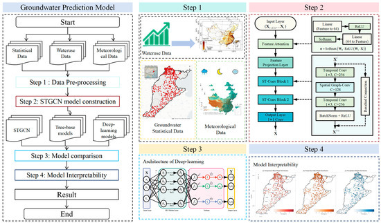
Figure 1. Groundwater level prediction flow chart.

(1)

Data acquisition: Data from groundwater monitoring wells, human water use, and meteorological data were collected from the study area to construct the original dataset.

(2)

Data preprocessing: The dataset was temporally split into training (80%) and testing (20%) subsets to evaluate model generalization. Specifically, the first 287 weeks (2018–2022) were used for training, and the remaining 72 weeks were reserved for testing, ensuring no information leakage from future observations.

(3)

Model Evaluation: Five key indicators (RMSE, MAE, R², MSE, and Pearson correlation coefficient) were used to conduct a comprehensive evaluation at both the overall and site levels, achieving a combination of macro performance evaluation and micro error diagnosis.

(4)

Interpretability analysis: By using attention mechanisms, the relative contributions of each driving factor to groundwater level prediction were quantitatively assessed, thereby providing insights into how environmental or anthropogenic factors at a specific location affect groundwater level changes.

2.2. Study Area

The North China Plain (NCP) is a large alluvial, multi-layered aquifer system located between the Taihang and Yanshan Mountains and the Bohai Bay, encompassing the provinces of Beijing, Tianjin, Shandong, Hebei, and Henan (Figure 2). Formed during Cenozoic tectonic movements, the plain consists of alternating coarse-grained fluvial sediments and fine-grained deltaic and lacustrine sediments, providing a typical scenario for studying the spatiotemporal evolution of groundwater levels under complex hydrogeological conditions. As China’s most important grain production base and densely populated area, the NCP faces severe water resource challenges. Long-term overexploitation has led to a continuous decline in shallow groundwater levels, forming multiple regional depressions. Dynamic monitoring and accurate prediction of water levels have become key scientific issues for the sustainable management of groundwater resources.

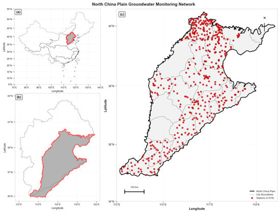
Figure 2. Overview map of the North China Plain. (a) shows the location of North China in China; (b) shows the plains area within North China; (c) shows the distribution of monitoring stations on the North China Plain.

2.3. Simulation Target and Hydrological Inputs

(1)

Groundwater level data.

Historical groundwater level data from the China Geological Environment Monitoring Center (CIGEM) covers water levels from 2005 to 2022. However, the time series records for most wells contain excessive gaps, making them unsuitable for modeling. After data quality screening, 518 observation wells with complete weekly groundwater level records spanning 359 weeks from 2018 to 2022 were selected, yielding a total of 185,962 observations for model training and evaluation. Figure 2 shows the spatial distribution of the study area and the selected observation wells in the shallow aquifer.

(2)

Water usage data

High-resolution sectoral water use data (HSWUD) can represent the spatiotemporal distribution characteristics of human water use activities (https://www.nature.com/articles/s41597-025-05400-2 (accessed on 5 November 2025)). This study uses provincial annual water use statistics, remote sensing land use data, population density distribution maps, reanalysis meteorological data, thermal power plant geographic information, and industrial enterprise micro-survey data to construct a monthly sectoral water use spatial distribution dataset with a 0.1° × 0.1° grid.

(3)

Meteorological data

ChinaMet is a comprehensive meteorological driven data product covering China (https://www.huanghe.ac.cn/metadata/21691d03-bef2-4800-924e-5614e7268b87 (accessed on 5 November 2025)), with high spatial resolution (1 km) and long time series (1980–2024). This dataset is developed using advanced data fusion techniques by integrating multi-source remote sensing observations, atmospheric reanalysis data, and field data from over 2000 surface meteorological stations. The ChinaMet dataset includes eight key meteorological elements: precipitation (pre), surface air temperature at 2 m (tmpmean), daily maximum temperature (tmpmax), daily minimum temperature (tmpmin), wind speed at 10 m (wind), relative humidity (rhu), surface pressure (pres), and potential evapotranspiration (pet).

2.4. STGCN Network Architecture

Based on the constructed graph structure, this paper proposes a comprehensive framework, MF-STGCN. As shown in Figure 3, MF-STGCN comprises four key components: data preprocessing, spatiotemporal graph construction, the STGCN module, and groundwater level prediction.

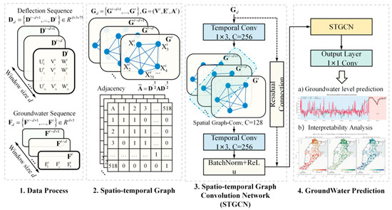
Figure 3. STGCN network structure. The framework consists of four main components: (1) Data processing of deflection and groundwater sequences with sliding window; (2) Spatio-temporal graph construction with normalized adjacency matrix; (3) Spatio-temporal graph convolution network with temporal convolution, spatial graph convolution, and residual connections; (4) Groundwater prediction module including (a) groundwater level prediction results and (b) interpretability analysis.

In the data preprocessing stage, the raw observation data from each monitoring station are organized into a structured time series, with water level measurement as the primary objective variable, supplemented by eight explanatory variables, including anthropogenic factors (irrigation water consumption, industrial water consumption, electricity consumption, and domestic water consumption) and hydrometeorological variables (potential evapotranspiration, precipitation, air pressure, and temperature). Training samples are extracted using the sliding window method, constructing an input tensor with dimensions (number of samples, 518, 12, 14), where 518 represents the number of monitoring stations, 12 represents the time step, and 14 represents the number of feature channels.

The spatiotemporal graph construction module utilizes the geographical coordinates (longitude, latitude, and altitude) of each monitoring station to construct a spatial adjacency matrix using a Gaussian kernel-weighted distance function, explicitly representing the spatial connectivity and interaction patterns between stations. The multi-source feature fusion module introduces an attention mechanism to achieve data-driven dynamic feature importance assessment and automatically learn the relative contribution of each input feature to groundwater level prediction.

The STGCN module adopts a “time–space–time” sandwich structure to collaboratively capture temporal evolution patterns and spatial propagation dynamics. Each STGCN block contains three sub-modules: (1) a temporal convolutional layer uses 1D causal convolution and gated linear units to extract temporal dependencies; (2) a spatial graph convolutional layer uses Chebyshev multinomial approximation to achieve spectral graph convolution and capture the spatial correlation encoded by the adjacency matrix; (3) a second temporal convolutional layer further refines the temporal features. The network uses batch normalization and residual connections to improve training stability and expressive power. Multiple STGCN blocks are stacked sequentially to gradually extract hierarchical spatiotemporal feature representations.

The output layer uses a fully connected layer to map the learned spatiotemporal features to groundwater level prediction values. MF-STGCN achieves end-to-end mapping from raw heterogeneous monitoring data to groundwater level prediction, and has stronger multi-source data processing and spatiotemporal modeling capabilities compared to traditional methods. Through the deep learning paradigm, the model can automatically learn complex nonlinear mapping relationships in the data, avoiding tedious manual feature engineering.

2.5. Machine Learning Algorithms

(1)

Convolutional Neural Networks (CNN)

Convolutional neural networks achieve automatic feature extraction and hierarchical representation through local connections, weight sharing, and spatial pooling [23]. Its core architecture consists of convolutional layers, pooling layers, and fully connected layers. The convolutional layer uses learnable convolution kernels to detect local features; the pooling layer downsamples features to reduce feature dimensionality and enhance translation invariance; and the fully connected layer integrates high-level features to complete the final task. The parameter sharing mechanism significantly reduces the number of model parameters and effectively mitigates overfitting.

(2)

Long Short-Term Memory (LSTM)

LSTM solves the gradient vanishing problem of traditional Recurrent neural network (RNN) through gating mechanism and memory unit, and realizes effective model of long-term dependencies [24]. It consists of three gate structures: the input gate controls the inflow of new information, the forget gate determines the retention of historical information, and the output gate adjusts the current output. The memory unit maintains stable gradient propagation through linear self-connections, enabling the network to selectively remember and forget information.

(3)

Extreme Gradient Boosting (XGBoost)

XGBoost is based on the gradient boosting decision tree, which iteratively trains weak learners to fit the residuals and forms a strong learner through weighted combination [25]. Key innovations include using second-order Taylor expansion to optimize the objective function; introducing L1/L2 regularization to prevent overfitting; implementing column sampling and row sampling to enhance generalization capabilities; and developing an efficient distributed parallel computing framework. The loss function is optimized by using a greedy algorithm to find the optimal split point and an approximate algorithm is used to process continuous features.

(4)

Random Forest (RF)

Random forest constructs multiple decorrelated decision trees through bootstrap sampling and random feature selection, and makes predictions by voting or averaging [26]. The double random mechanism effectively reduces model variance and improves generalization performance. It provides unbiased generalization error estimation through out-of-bag error, calculates feature importance for feature selection, and is robust to high-dimensional data and feature correlation.

2.6. Computational Environment

All models were implemented using Python 3.9 and PyTorch 1.12.0 frameworks. Experiments were conducted on a workstation equipped with an Intel Core i9-10900K CPU, 64 GB of RAM, and an NVIDIA GeForce RTX 3090 GPU (24 GB of VRAM), running Windows 11.

3. Results and Discussion

3.1. Time Window and Prediction Length Analysis

The time window length, as a key hyperparameter that determines the amount of effective historical information in the model input sequence, has a significant impact on the prediction performance of the STGCN model. As shown in Figure 4, this study systematically evaluated the impact of five different time window lengths (7, 12, 18, 32, and 64 weeks) on the model prediction accuracy. Experimental results show that when the input time step is extended from 7 weeks to 12–18 weeks, the model performance is stable and excellent: the RMSE and MAE both remain at low levels (RMSE: 0.2510 ± 0.2243, MAE: 0.1666 ± 0.1428), the R² value remains stable in the high range of 0.80–0.95, and the correlation coefficient is close to 1.0. In particular, under the 12-week window configuration, the model shows the best performance stability, with the smallest interquartile range of various indicators and the least outliers. However, when the time window was further extended to 32 weeks and 64 weeks, the model performance deteriorated sharply. As shown in Table 1, compared with the 7-day baseline, the 32-week input leads to a 453.71% worsening of RMSE, a 666.38% worsening of MAE, and a 1071.64% decrease in R². The performance degradation of 64-week input is even more serious, with various error indicators deteriorating by more than 400%. More importantly, the stability of the model decreases significantly over long time windows, as evidenced by a significant increase in the dispersion of the R² value and correlation coefficient, and the appearance of a large number of outliers. This phenomenon indicates that overly long historical sequences introduce redundant information and noise that are irrelevant to the current prediction task, interfering with the model’s ability to extract key spatiotemporal features. Therefore, considering both prediction accuracy and computational efficiency, a time window length of 12–18 weeks provides the optimal performance balance point for the STGCN model.

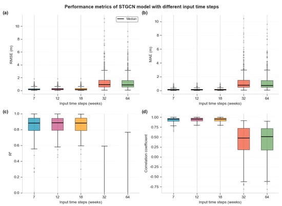
Figure 4. Analysis of the impact of different time window sizes (7, 12, 18, 32, 64). (a) Distribution of RMSE for different input time steps; (b) Distribution of MAE for different input time steps; (c) Distribution of R² for different input time steps; (d) Distribution of correlation coefficient for different input time steps.

Table 1. Performance improvement analysis (compared to 7-day input).

Input Days	RMSE (%)	MAE (%)	R2 (%)	Correlation (%)
7	Baseline	Baseline	Baseline	Baseline
12	−1.26%	−5.07%	+1.09%	+0.59%
18	+0.68%	−0.88%	+1.38%	+0.51%
32	−453.71%	−666.38%	−1071.64%	−57.44%
64	−448.56%	−655.21%	−1598.24%	55.98%

As another key factor affecting the performance of the STGCN model, the prediction time has an obvious decreasing trend in its impact on the accuracy of shallow groundwater level prediction. As shown in Figure 5, this study systematically evaluated the impact of six different prediction horizons (1, 2, 3, 4, 5, and 7 weeks) on model performance. Experimental results show that as the prediction time increases, the model performance shows a monotonically decreasing trend. Specifically, when the prediction period is one week, the model performs best, with the medians of RMSE and MAE being 0.26 m and 0.17 m, respectively, the mean R² reaching 0.8565 ± 0.1055, and the correlation coefficient as high as 0.9395 ± 0.0472, indicating that the model can accurately capture the short-term groundwater level variation characteristics. As the forecast period gradually extends to 7 weeks, all performance indicators show a significant deterioration: RMSE increases to 0.6213 ± 0.5114 m (an increase of 143%), MAE increases to 0.4395 ± 0.3610 m (an increase of 151%), R² decreases to 0.1739 ± 0.5863 (a decrease of 79.7%), and the correlation coefficient decreases to 0.6862 ± 0.1766 (a decrease of 27.0%).

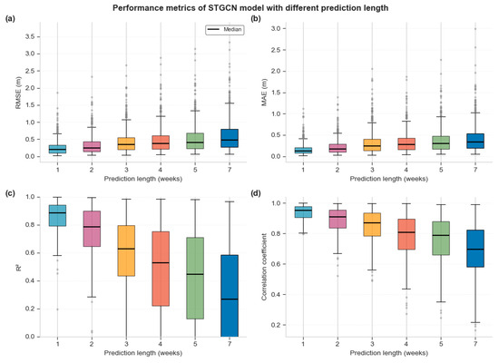
Figure 5. Impact of different prediction lengths on prediction metrics (1, 2, 3, 4, 5, 6, 7). (a) Distribution of RMSE for different prediction lengths; (b) Distribution of MAE for different prediction lengths; (c) Distribution of R²; for different prediction lengths; (d) Distribution of correlation coefficient for different prediction lengths.

It is worth noting that the attenuation of groundwater level prediction performance shows nonlinear characteristics. As shown in Table 2, within the short-term prediction range of 1–3 weeks, the performance degradation is relatively gentle, with the R² value gradually decreasing from 0.8565 to 0.5093, which remains at an acceptable level. This indicates that the model can effectively capture the short-term dynamic response characteristics of the groundwater system. However, when the prediction period exceeds 3 weeks, the performance decay accelerates significantly, and the R² values for 4–7 weeks drop sharply to 0.3694, 0.3084, and 0.1739. In addition, as the forecast period increases, the uncertainty of the model forecast increases significantly, which is manifested in the continued expansion of the standard deviation of various indicators. In particular, the standard deviation of R² is as high as 0.5863 for the 7-week forecast, indicating that the model is seriously insufficient in stability in long-term forecasts. Therefore, it is recommended to control the prediction time within 3 weeks in actual groundwater level prediction applications to ensure the reliability and practicality of the prediction results.

Table 2. Statistical summary of STGCN model performance metrics.

Prediction Metrics (Weeks)	RMSE (%)	MAE (%)	R2 (%)	Correlation (%)
	Mean ± SD	Mean ± SD	Mean ± SD	Mean ± SD
1	0.2558 ± 0.2271	0.1735 ± 0.1532	0.8565 ± 0.1055	0.9395 ± 0.0472
2	0.3361 ± 0.2914	0.2263 ± 0.1901	0.7399 ± 0.2432	0.8922 ± 0.0790
3	0.4512 ± 0.3779	0.3363 ± 0.3023	0.5093 ± 0.5407	0.8512 ± 0.1035
4	0.4889 ± 0.4060	0.3448 ± 0.2685	0.3694 ± 0.7666	0.7872 ± 0.1363
5	0.5320 ± 0.4479	0.3767 ± 0.3000	0.3084 ± 0.6721	0.7606 ± 0.1502
7	0.6213 ± 0.5114	0.4395 ± 0.3610	0.1739 ± 0.5863	0.6862 ± 0.1766

Experimental results show that the model is significantly sensitive to the amount of temporal context information and the difficulty of the prediction task. By setting a 12-week time window, the model finds the best balance between retaining sufficient historical data and avoiding the introduction of noise/redundancy. As the forecast horizon increases, forecast uncertainty naturally accumulates, leading to performance degradation, with the model showing its highest reliability in short-term forecasts (1–3 weeks).

3.2. Comparison of Model Prediction Accuracy

This study systematically evaluated the performance of the STGCN model and four benchmark models (CNN, LSTM, Random Forest, and XGBoost) in shallow groundwater level prediction in the North China Plain. As shown in Figure 6a, in the long-term series forecast from 2018 to 2022, all models can capture the overall trend of groundwater level changes, but there are significant differences in the prediction accuracy during the test period (red shaded area). From the box plot in Figure 6b, it can be seen intuitively that STGCN and LSTM are significantly better than other models in the distribution of prediction errors, showing smaller medians and more concentrated interquartile ranges. Although traditional machine learning methods (RF and XGBoost) have certain predictive capabilities, they are difficult to effectively model complex spatiotemporal dependencies; the prediction error distribution of the CNN model is the most dispersed, indicating that it has obvious limitations when processing groundwater level spatiotemporal data.

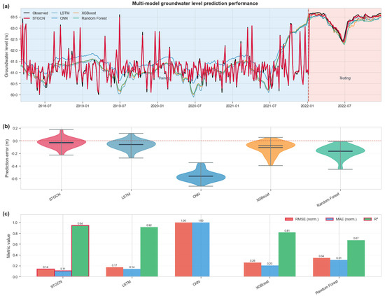
Figure 6. Performance evaluation of groundwater level prediction models in the North China Plain: time series evolution (a), error distribution (b), and overall accuracy index comparison (c).

The quantitative analysis in Table 3 and Figure 6c fully verifies the superiority of the STGCN model. In terms of prediction accuracy, the RMSE of STGCN is 0.256 ± 0.227 m, which is comparable to LSTM (0.257 ± 0.220 m), but significantly better than CNN (0.704 ± 0.725 m), RF (0.420 ± 0.358 m), and XGBoost (0.346 ± 0.378 m), with error reductions of 63.6%, 39.0%, and 26.0%, respectively. More importantly, STGCN achieves an R² index of 0.857 ± 0.106, which is higher than LSTM’s 0.839 ± 0.155, showing stronger explanatory power. It is worth noting that the correlation coefficient of STGCN is as high as 0.940 ± 0.047, which not only has the highest value but also the smallest standard deviation (0.047), which fully demonstrates that the prediction stability and reliability of the model are optimal in different monitoring wells and time periods. In contrast, although the CNN model has a higher correlation coefficient (0.926 ± 0.064), its R² value is negative (−0.986 ± 4.573), indicating that the model has a serious overfitting problem.

Table 3. Statistical summary of different model performance metrics.

Models	RMSE (%)	MAE (%)	R2 (%)	Correlation (%)
	Mean ± SD	Mean ± SD	Mean ± SD	Mean ± SD
STGCN	0.2558 ± 0.2271	0.1735 ± 0.1532	0.8565 ± 0.1055	0.9395 ± 0.0472
CNN	0.7037 ± 0.7249	0.6464 ± 0.7129	−0.9864 ± 4.5731	0.9255 ± 0.0643
LSTM	0.2571 ± 0.2204	0.1757 ± 0.1464	0.8388 ± 0.1546	0.9349 ± 0.0526
RF	0.4196 ± 0.3583	0.3157 ± 0.2893	0.5129 ± 0.9454	0.8601 ± 0.1303
XGB	0.3463 ± 0.3783	0.2159 ± 0.2227	0.3973 ± 2.3113	0.8761 ± 0.1995
STGCN	0.2558 ± 0.2271	0.1735 ± 0.1532	0.8565 ± 0.1055	0.9395 ± 0.0472

From the perspective of multi-source data fusion, STGCN effectively integrates heterogeneous data such as meteorology, hydrology, and geology through a graph neural network architecture, achieving a comprehensive characterization of the groundwater system. The comparison of various performance indicators in Figure 6c clearly demonstrates the advantages of this fusion strategy: STGCN achieves optimal or near-optimal levels in the three core indicators of RMSE (0.14 m), MAE (0.11 m), and R² (0.94). In particular, compared with LSTM that only relies on time series features, STGCN is able to capture the hydraulic connections between monitoring wells by introducing spatial topological structure learning, thereby providing more accurate regional groundwater level predictions. This spatiotemporal collaborative modeling capability is of great significance for groundwater management in large-scale regions such as the North China Plain, and provides reliable technical support for water resource allocation and drought and flood warning.

3.3. Model Interpretability: Feature Attention Weight Analysis

Through attention mechanism and feature importance analysis (Figure 7), this study reveals how the model integrates multi-source environmental variables to capture the complex dynamic characteristics of the groundwater system.

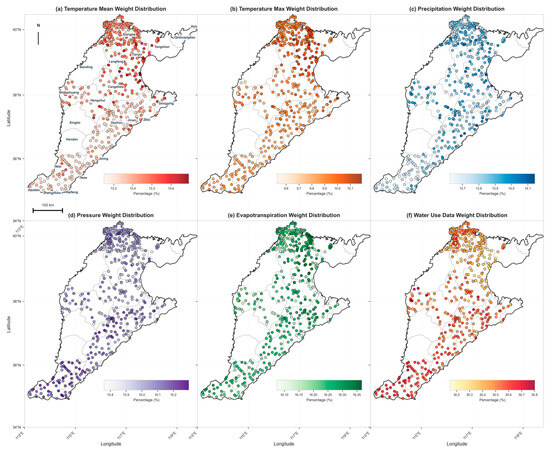
Figure 7. Spatial Distribution Map of Predictive Variables Affecting Water Levels at Groundwater Monitoring Stations in the North China Plain.

The spatial weight distribution of temperature variables (Figure 7a,b) shows significant regional heterogeneity. The average temperature attention weight shows relatively high values in the northern and central plains (13.5~3.7%), reflecting the sensitivity of groundwater systems in these regions to temperature regulation. The spatial pattern of the highest temperature weights further reinforces this pattern, especially in the central and northern parts where a clear high-value cluster is formed (9.8–0.1%), indicating that the model identifies the physical mechanism by which extreme temperature conditions regulate groundwater dynamics by affecting evapotranspiration intensity. This spatial heterogeneity reflects the model’s ability to adaptively learn the temperature-groundwater coupling relationship under different hydrogeological conditions. The spatial distribution of precipitation weights (Figure 7c) shows a relatively homogeneous characteristic, reflecting the universality of precipitation recharge as the dominant driving force of the groundwater system. The slightly higher weight values in the eastern coastal areas suggest that the model captures the rapid response characteristics of the shallow aquifer system to precipitation events. The air pressure variable (Figure 7d) shows a clear latitudinal gradient, ranging from 15.8% in the south to 16.2% in the north. This spatial pattern may reflect the differentiated impact of large-scale atmospheric circulation on regional groundwater dynamics identified by the model. The evapotranspiration weight (Figure 7e) remains relatively stable at a moderate level (16.2–16.35%) across the entire domain, and its spatial uniformity indicates that evapotranspiration, as a key pathway for groundwater discharge, is of consistent importance at the regional scale.

The most important finding is the significant spatial variability in water use data (Figure 7f). The model assigns significantly higher attention weights (>30.6%) to urbanized areas (such as those surrounding Jinan and Zhengzhou), while agricultural irrigation-dominated areas receive a moderate weight (0.4–0.5%). This spatial differentiation clearly demonstrates that the model successfully learns the nonlinear relationship between human activity intensity and groundwater response, highlighting the advantages of deep learning models in capturing the complexity of coupled social-hydrological systems.

4. Discussion

4.1. Optimal Time Configuration for Groundwater Level Prediction

The sensitivity of the STGCN model to temporal configuration parameters reveals fundamental insights into the hydrodynamic response characteristics of shallow groundwater systems. Our results suggest that the optimal time window of 12–18 weeks represents a critical time scale to balance information adequacy and noise minimization in the hydrogeological context of the North China Plain. This time frame covers the complete seasonal cycle, effectively capturing the complex precipitation-recharge dynamics while filtering out confounding interannual variability that could affect prediction accuracy.

The drastic performance drop observed when extending the time window to 32–64 weeks (RMSE drops by more than 400%) reveals a critical threshold in the “hydrogeological memory” of the groundwater system. This phenomenon can be attributed to several interrelated factors. First, the relatively high hydraulic conductivity of the shallow aquifers in the North China Plain causes the hydrological signal to dissipate rapidly, making historical data outside of seasonal timescales increasingly less relevant to the current state of the system. Second, the introduction of extended historical series introduces what we call “temporal aliasing,” where outdated hydrological patterns that have already equilibrated with the system inadvertently act as predictive noise rather than informative signals. This finding is consistent with the concept of effective information horizon in complex dynamical systems, suggesting that groundwater systems have inherent temporal boundaries beyond which historical information becomes detrimental rather than beneficial to the prediction task.

Model performance exhibits a nonlinear decay with increasing prediction horizon, reflecting the fundamental stochastic nature of groundwater dynamics over extended time scales. The relatively robust performance (R² > 0.5) within the 1–3 week prediction window indicates that short-term groundwater changes are mainly controlled by deterministic hydrogeological processes, including Darcy flow mechanics and the principle of mass conservation. However, the sharp decline in forecast ability beyond the three-week threshold reveals the emergence of cascading uncertainties. These uncertainties arise from a variety of factors: the inherent stochasticity of meteorological forcing, which increases over longer time horizons; the non-stationarity of anthropogenic factors (particularly agricultural irrigation patterns); and the potential for extreme events that fall outside the range of the model’s learned probability distribution. This observation confirms the theoretical framework of the limits of hydrological predictability, suggesting the existence of a fundamental temporal boundary beyond which deterministic predictions transition to probabilistic estimates.

4.2. Advantages of Spatiotemporal Graph Neural Networks

The advantages of the STGCN framework over traditional methods mainly stem from its ability to simultaneously simulate the temporal dynamics and spatial interdependencies of groundwater systems. While the performance improvements of STGCN compared to LSTM (2.1% improvement in R² and 31.7% reduction in standard deviation) may seem small in absolute terms, they represent a meaningful methodological advancement in groundwater modeling approaches. STGCN explicitly incorporates spatial topology through graph convolution operations, breaking through the limitations of pure temporal models and being able to capture the inherent hydraulic connectivity patterns of groundwater flow systems. This spatial awareness capability is particularly important in regional-scale water resource management, as improved forecast stability directly translates into increased confidence in decision-making.

The suboptimal performance of traditional machine learning algorithms (RF: R² = 0.513, XGBoost: R² = 0.397) highlights the fundamental inadequacy of the independence assumption in groundwater modeling. Although these methods have been proven effective in numerous prediction tasks, they fail to account for the inherent spatiotemporal autocorrelations in hydrogeological systems. The spatial continuity of hydraulic head distribution and the temporal persistence of groundwater flow patterns violate the independent and identically distributed (i.i.d.) assumptions on which these algorithms are based. Particularly noteworthy is the catastrophic failure of the CNN model (negative R² of −0.986 ± 4.573), which exposes the fundamental incompatibility between conventional convolution operations and the irregular spatial topology of the groundwater monitoring network. Unlike image data with a uniform pixel grid, groundwater monitoring wells are distributed according to hydrogeological significance and accessibility constraints, resulting in a heterogeneous spatial structure that cannot be effectively represented by standard convolution kernels.

4.3. Physical Insights from Attention Weight Analysis

The spatial distribution patterns of feature attention weights provide unprecedented quantitative insights into the hierarchical control mechanisms of groundwater dynamics in the North China Plain. The dominance of water consumption data in the regime of interest, especially in densely populated urban centers, quantitatively validates the hypothesis that the groundwater system in the region has shifted from natural dominance to anthropogenic control.

The unusually high weight of concern for water use in Anyang (30.6–30.7%) deserves special attention, as this likely reflects the intensive industrial and agricultural water use characteristics of the region. The spatial heterogeneity of feature importance suggests that a unified water resource management strategy for the entire North China Plain may not be optimal; instead, context-specific policies that take into account the intensity of local anthropogenic pressures should be prioritized. The model is able to automatically identify these regional differences through an attention mechanism, demonstrating its potential as a decision support tool for spatially differentiated water resources management.

The contrasting spatial patterns between the weights of lagged and real-time meteorological data reveal the complex interactions between hydrogeological properties and climate forcing mechanisms. The increase in real-time meteorological weights over the northern part of the North China Plain may reflect the characteristics of the thickness of the shallow vadose zone in these areas, which promotes rapid infiltration and immediate response of groundwater to precipitation events. In contrast, the central part of the North China Plain has a higher reliance on lagged meteorological data, indicating the presence of a thicker unsaturated zone, which leads to a significant time delay in the precipitation-recharge relationship. This spatial variation in temporal response characteristics highlights the importance of incorporating hydrogeological heterogeneity in regional-scale groundwater modeling efforts. The attention mechanism can automatically detect and quantify these spatially varying response patterns, which is a significant improvement over traditional modeling methods that often assume consistent response characteristics across large regions.

5. Conclusions

In this study, a spatiotemporal graph convolutional network (STGCN) framework based on multi-source data fusion was developed for the dynamic prediction of shallow groundwater levels in the North China Plain. By systematically integrating multi-source heterogeneous data such as meteorology, hydrology, and human activities, the study compared different prediction models, interpreted the feature attention weight distribution for enhanced interpretability, and evaluated the spatial generalization ability of the model. The systematic study yielded the following main conclusions: (1) the STGCN model significantly outperformed traditional methods in terms of prediction accuracy and stability, with RMSE reduced to 0.256 ± 0.227 m and R² reaching 0.857 ± 0.106. Compared with benchmark models such as CNN, random forest, and XGBoost, the error was reduced by 26–64%; (2) the 12–18 week time window is identified as the optimal length of historical information, which can fully capture the characteristics of the seasonal hydrological cycle while avoiding the introduction of noise information that is decoupled from the current system state; (3) the model showed the highest reliability (R² > 0.5) in short-term predictions of 1–3 weeks, while the uncertainty of predictions increased significantly after 3 weeks, revealing the time threshold of groundwater system predictability; (4) the attention mechanism analysis quantitatively confirmed that human activities have become the dominant factor in the groundwater dynamics in the North China Plain. The average weight of water resource utilization data reached the highest level and was more prominent in densely populated areas, while the influence of meteorological factors showed significant spatial heterogeneity.

This study provides important technical support for sustainable groundwater management in the North China Plain and other water-scarce areas. The optimal time configuration parameters identified by the model can directly guide the optimization design of the monitoring network and the formulation of data collection strategies; the spatially differentiated feature importance analysis provides a scientific basis for formulating water resources management policies tailored to local conditions; and the high reliability of short-term predictions enables their direct application in real-time water resources scheduling and drought and flood warning systems. In addition, the method framework established in this study has good scalability and can be extended to other environmental prediction problems with networked monitoring systems by adjusting the graph structure definition and feature engineering.

However, this study still has several limitations that provide directions for future research. The degradation of long-term prediction performance needs to be addressed through physical constraints or hybrid modeling approaches; coupled prediction of multi-layer aquifer systems has not yet been achieved; and the model’s ability to migrate across regions requires further verification. Future research should focus on exploring cutting-edge technologies such as physical information neural networks, uncertainty quantification, and causal inference to build a more robust, interpretable, and physically consistent groundwater prediction system.

References

- Fernández-Ortega, J.; Barberá, J.A.; Andreo, B. Real-time karst groundwater monitoring and bacterial analysis as early warning strategies for drinking water supply contamination. Sci. Total Environ. 2024, 912, 169539. [Google Scholar] [CrossRef]
- Ouyang, L.; Zhao, Z.; Zhou, D.; Cao, J.; Qin, J.; Cao, Y.; He, Y. Study on the relationship between groundwater and land subsidence in Bangladesh Combining GRACE and InSAR. Remote Sens. 2024, 16, 3715. [Google Scholar] [CrossRef]
- Hemid, E.M.; Kántor, T.; Tamma, A.A.; Masoud, M.A. Effect of groundwater fluctuation, construction, and retaining system on slope stability of Avas Hill in Hungary. Open Geosci. 2021, 13, 1139–1157. [Google Scholar] [CrossRef]
- Dai, Z.; Peng, L.; Qin, S. Experimental and numerical investigation on the mechanism of ground collapse induced by underground drainage pipe leakage. Environ. Earth Sci. 2024, 83, 32. [Google Scholar] [CrossRef]
- Leaf, A.T.; Fienen, M.N. Modflow-setup: Robust automation of groundwater model construction. Front. Earth Sci. 2022, 10, 903965. [Google Scholar] [CrossRef]
- Fiorese, G.D.; Balacco, G.; Bruno, G.; Nikolaidis, N. Hydrogeological modelling of a coastal karst aquifer using an integrated SWAT-MODFLOW approach. Environ. Model. Softw. 2025, 183, 106249. [Google Scholar] [CrossRef]
- Yeganeh, A.; Ahmadi, F.; Wong, Y.J.; Shadman, A.; Barati, R.; Saeedi, R. Shallow vs. deep learning models for groundwater level prediction: A multi-piezometer data integration approach. Water Air Soil Pollut. 2024, 235, 441. [Google Scholar] [CrossRef]
- Farshad, H.; Shourian, M.; Salehi, M.J. Entropy-based groundwater quality monitoring network design using a simulation–optimization approach by coupling genetic algorithm, MODFLOW and MT3DMS. J. Hydroinform. 2025, 27, 159–177. [Google Scholar] [CrossRef]
- Saqr, A.M.; Nasr, M.; Fujii, M.; Yoshimura, C.; Ibrahim, M.G. Optimal Solution for Increasing Groundwater Pumping by Integrating MODFLOW-USG and Particle Swarm Optimization Algorithm: A Case Study of Wadi El-Natrun, Egypt. In Proceedings of the International Conference on Environment Science and Engineering, Beijing, China, 2–5 September 2022; pp. 59–73. [Google Scholar]
- Kontos, Y.N.; Rompis, I.; Karpouzos, D. Optimal pollution control and pump-and-fertilize strategies in a nitro-polluted aquifer, using Genetic Algorithms and Modflow. Agronomy 2023, 13, 1534. [Google Scholar] [CrossRef]
- Rohde, M.M.; Biswas, T.; Housman, I.W.; Campbell, L.S.; Klausmeyer, K.R.; Howard, J.K. A machine learning approach to predict groundwater levels in California reveals ecosystems at risk. Front. Earth Sci. 2021, 9, 784499. [Google Scholar] [CrossRef]
- Malakar, P.; Mukherjee, A.; Bhanja, S.N.; Ray, R.K.; Sarkar, S.; Zahid, A. Machine-learning-based regional-scale groundwater level prediction using GRACE. Hydrogeol. J. 2021, 29, 1027–1042. [Google Scholar] [CrossRef]
- Nourani, V.; Khodkar, K.; Gebremichael, M. Uncertainty assessment of LSTM based groundwater level predictions. Hydrol. Sci. J. 2022, 67, 773–790. [Google Scholar] [CrossRef]
- Liu, W.; Yu, H.; Yang, L.; Yin, Z.; Zhu, M.; Wen, X. Deep learning-based predictive framework for groundwater level forecast in arid irrigated areas. Water 2021, 13, 2558. [Google Scholar] [CrossRef]
- Deng, Y.; Ye, X.; Du, X. Predictive modeling and analysis of key drivers of groundwater nitrate pollution based on machine learning. J. Hydrol. 2023, 624, 129934. [Google Scholar] [CrossRef]
- Wei, A.; Chen, Y.; Li, D.; Zhang, X.; Wu, T.; Li, H. Prediction of groundwater level using the hybrid model combining wavelet transform and machine learning algorithms. Earth Sci. Inform. 2022, 15, 1951–1962. [Google Scholar] [CrossRef]
- Jalalkamali, A. Using of hybrid fuzzy models to predict spatiotemporal groundwater quality parameters. Earth Sci. Inform. 2015, 8, 885–894. [Google Scholar] [CrossRef]
- Nourani, V.; Mousavi, S. Spatiotemporal groundwater level modeling using hybrid artificial intelligence-meshless method. J. Hydrol. 2016, 536, 10–25. [Google Scholar] [CrossRef]
- Sakizadeh, M.; Mohamed, M.M.A.; Klammler, H. Trend analysis and spatial prediction of groundwater levels using time series forecasting and a novel spatio-temporal method. Water Resour. Manag. 2019, 33, 1425–1437. [Google Scholar] [CrossRef]
- Nourani, V.; Mogaddam, A.A.; Nadiri, A.O. An ANN-based model for spatiotemporal groundwater level forecasting. Hydrol. Process. 2008, 22, 5054–5066. [Google Scholar] [CrossRef]
- Seo, J.Y.; Lee, S.-I. Predicting changes in spatiotemporal groundwater storage through the integration of multi-satellite data and deep learning models. IEEE Access 2021, 9, 157571–157583. [Google Scholar] [CrossRef]
- Pagendam, D.; Janardhanan, S.; Dabrowski, J.; MacKinlay, D.J. A log-additive neural model for spatio-temporal prediction of groundwater levels. Spat. Stat. 2023, 55, 100740. [Google Scholar] [CrossRef]
- Li, Z.; Liu, F.; Yang, W.; Peng, S.; Zhou, J. A survey of convolutional neural networks: Analysis, applications, and prospects. IEEE Trans. Neural Netw. Learn. Syst. 2021, 33, 6999–7019. [Google Scholar] [CrossRef]
- Hochreiter, S.; Schmidhuber, J. Long short-term memory. Neural Comput. 1997, 9, 1735–1780. [Google Scholar] [CrossRef] [PubMed]
- Chen, T.; Guestrin, C. Xgboost: A Scalable Tree Boosting System. In Proceedings of the 22nd ACM SIGKDD International Conference on Knowledge Discovery and Data Mining, San Francisco, CA, USA, 13–17 August 2016; pp. 785–794. [Google Scholar]
- Breiman, L. Random forests. Mach. Learn. 2001, 45, 5–32. [Google Scholar] [CrossRef]
Disclaimer/Publisher’s Note: The statements, opinions and data contained in all publications are solely those of the individual author(s) and contributor(s) and not of MDPI and/or the editor(s). MDPI and/or the editor(s) disclaim responsibility for any injury to people or property resulting from any ideas, methods, instructions or products referred to in the content. |
© 2025 by the authors. Licensee MDPI, Basel, Switzerland. This article is an open access article distributed under the terms and conditions of the Creative Commons Attribution (CC BY) license (https://creativecommons.org/licenses/by/4.0/).