From Black Box to Transparency: An Explainable Machine Learning (ML) Framework for Ocean Wave Prediction Using SHAP and Feature-Engineering-Derived Variable

Abstract

Accurate prediction of significant wave height (SWH) is central to coastal ocean dynamics, wave–climate assessment, and operational marine forecasting, yet many high-performing machine-learning (ML) models remain opaque and weakly connected to underlying wave physics. We propose an explainable, feature engineering-guided ML framework for coastal SWH prediction that combines extremal wave statistics, temporal descriptors, and SHAP-based interpretation. Using 30 min buoy observations from a high-energy, wave-dominated coastal site off Australia’s Gold Coast, we benchmarked seven regression models (Linear Regression, Decision Tree, Random Forest, Gradient Boosting, Support Vector Regression, K-Nearest Neighbors, and Neural Networks) across four feature sets: (i) Base (Hmax, Tz, Tp, SST, peak direction), (ii) Base + Temporal (lags, rolling statistics, cyclical hour/month encodings), (iii) Base + a physics-informed Wave Height Ratio, WHR = Hmax/Hs, and (iv) Full (Base + Temporal + WHR). Model skill is evaluated for full-year, 1-month, and 10-day prediction windows. Performance was assessed using R², RMSE, MAE, and bias metrics, with the Technique for Order Preference by Similarity to Ideal Solution (TOPSIS) employed for multi-criteria ranking. Inclusion of WHR systematically improves performance, raising test R² from a baseline range of ~0.85–0.95 to values exceeding 0.97 and reducing RMSE by up to 86%, with a Random Forest|Base + WHR configuration achieving the top TOPSIS score (1.000). SHAP analysis identifies WHR and lagged SWH as dominant predictors, linking model behavior to extremal sea states and short-term memory in the wave field. The proposed framework demonstrates how embedding simple, physically motivated features and explainable AI tools can transform black-box coastal wave predictors into transparent models suitable for geophysical fluid dynamics, coastal hazard assessment, and wave-energy applications.

1. Introduction

Accurate prediction of ocean surface waves, particularly significant wave height (SWH), is fundamental for understanding and managing a wide range of geophysical fluid processes in the coastal ocean. The ocean covers approximately 70–71% of the Earth’s surface, and its dynamic processes, including waves, have a substantial impact on climate, environment, and ecosystems [1,2,3]. Accurate prediction of SWH is fundamental to understanding coastal ocean dynamics, assessing wave–climate variability, managing coastal hazards, and supporting operational marine forecasting systems [4,5]. It serves as a primary descriptor of sea state conditions and plays a critical role in applications ranging from maritime navigation safety and offshore infrastructure design to wave energy resource assessment and coastal zone management [6,7]. In high-energy, wave-dominated coastal environments, where extreme wave events can trigger coastal flooding, beach erosion, and structural damage [8,9], reliable short-term SWH forecasting has become increasingly essential for early warning systems and risk mitigation strategies [10].

SWH is a key bulk descriptor of the wave field, governing wave energy flux, momentum transfer, and air–sea interaction [11,12]. Accurate SWH prediction is crucial for:

i.

Marine engineering and construction: SWH is a primary consideration in the design, planning, and operation of coastal and offshore structures, including oil platforms, harbors, and submarine pipelines [13,14,15,16].

ii.

Navigation safety: Reliable SWH forecasts provide essential environmental information for ship navigation and offshore operations, improving safety and efficiency [17,18].

iii.

Marine disaster assessment and prevention: SWH prediction is vital for disaster warning and mitigation, especially in regions affected by complex atmospheric processes such as monsoons and cyclones [19,20,21].

iv.

Renewable energy utilization: Wave energy is directly proportional to the square of SWH, making its prediction essential for evaluating wave power potential and optimizing the operation of wave energy converters (WECs) [22,23,24,25,26].

v.

Climate studies: SWH is used to assess climate change impacts, such as coastal erosion, storm generation, and changes in storm frequency and intensity [16].

Traditionally, the forecasting of ocean waves has been dominated by process-based numerical models, such as SWAN and WAVEWATCH III. These models solve deterministic physical equations to simulate wave generation, propagation, and dissipation. While valuable for understanding oceanic processes, they are often constrained by their computational expense, sensitivity to boundary conditions, and challenges in capturing the full spectrum of non-linear and stochastic wave dynamics, especially for operational, short-term forecasting [27,28,29,30,31].

All these models require substantial computational resources and memory, especially for high-resolution or long-term simulations, which can limit their practical application in operational settings where rapid results are needed [32]. Accurate forecasts depend on detailed terrain, wind field, and boundary condition data. The complexity of the calculation methods and the need for extensive calibration further increase computational time and uncertainty [28]. These models can struggle to fully represent the non-linear and stochastic nature of ocean waves, particularly under rapidly changing meteorological conditions or in semi-enclosed basins like the Mediterranean Sea, where local wind effects and seasonal variability introduce additional challenges [33].

A growing body of research highlights the transformative potential of feature engineering, especially the creation of input variables informed by physical principles, to enhance model performance and generalizability [34]. Despite this, the majority of ML-based SWH forecasting studies rely on raw variables such as wind speed, wave period, and direction, often neglecting derived, physics-informed indices that encapsulate non-linear interactions and extremal behaviors [35,36]. Furthermore, the pursuit of predictive accuracy has frequently come at the expense of transparency, resulting in “black-box” models that are ill-suited for decision-critical applications in energy and coastal management, where understanding the rationale behind predictions is as vital as the predictions themselves [37]. For practitioners, explainability is essential for informing design tolerances, operational strategies, and risk assessments in dynamic marine environments [38].

Machine learning (ML) methods have emerged as powerful alternatives or supplements to traditional wave prediction models due to their ability to construct non-linear mapping relationships, which can significantly improve prediction accuracy, especially for wave heights at fixed locations [39]. ML models are computationally efficient, require less computational resources, and are particularly suitable for real-time wave prediction due to their advantages in handling non-linear, non-smooth time series [40]. These models can analyze vast datasets, learn complex patterns, and make accurate predictions, offering a low-cost and efficient approach to wave height forecasting [41].

Most ML applications in wave prediction treat the problem as a statistical mapping from raw inputs (such as wind speed, significant wave height, and characteristic periods) to outputs like significant wave height (SWH), without incorporating physical knowledge of wave statistics or dynamics [42,43]. Several studies note that ML models are often used to construct non-linear mapping relationships for wave height prediction, but these models typically do not explain results through physical mechanisms or embed physical laws into their structure. Consequently, these predictions are often not directly interpretable in terms of underlying wave physics, and typically require expert validation to ensure alignment with physical principles.

Feature engineering is consistently described as a critical step in the machine learning workflow, involving the selection, transformation, and creation of input variables to enhance model predictive performance, robustness, and interpretability [44,45,46,47,48]. This process bridges raw data and predictive capability by extracting, transforming, and optimizing features using domain expertise and data analysis techniques. Feature engineering encompasses both feature selection (identifying and retaining the most relevant features) and feature extraction (transforming or combining features to create new, more informative variables) [49,50].

Feature engineering has been shown to enhance model accuracy, reduce overfitting, and improve generalization, especially when expert-designed features are used for complex systems such as time-series production data or bearing fault diagnosis [51,52,53]. By selecting more representative features, model complexity can be reduced, leading to simpler and more generalizable models [44,52]. The effectiveness of feature engineering often surpasses the impact of algorithm choice; even robust models like Random Forests benefit significantly from high-quality feature engineering [54]. Feature selection methods that retain original features without altering their values help maintain interpretability, making it easier to understand model behavior [55]. Encoding known physical relationships into features not only improves performance but also makes model outputs more interpretable and aligned with domain knowledge [56]. Techniques such as SHAP-based interpretability and model-agnostic variable ranking (e.g., NCAR) are used to identify influential features and explain model decisions [57].

ML models, especially complex ones such as tree ensembles and neural networks [58], are often considered “black boxes” due to their opaque internal mechanisms, making them difficult to interpret even when physics-informed features are included [59,60,61,62,63,64,65]. This lack of transparency is a significant challenge in fields like coastal hazard assessment, wave energy planning, and climate services, where end-users require not only accurate predictions but also an understanding of the model’s behavior across different regimes (e.g., calm conditions, storms, seasonal transitions, or shifts in wave direction) [59,65]. The inability to interpret ML model decisions can hinder trust and adoption among stakeholders, as understanding the rationale behind predictions is crucial for informed decision-making, especially in high-stakes or regulated environments [66,67,68]. In coastal and climate applications, this is particularly important because decisions based on model outputs can have significant financial, environmental, and safety consequences [59,61,63,65].

Despite rapid methodological advances, two critical gaps persist in the literature. First, there is a lack of exploration into the effects of different input features, including engineered features, on model performance, which limits the ability to fully understand and optimize machine learning models. This gap also extends to insufficient efforts to demystify the black-box nature of these models, as most studies do not provide comprehensive insights into how various features influence outcomes, despite some attempts using global-level sensitivity or parametric analysis [69]. Second, while multi-criteria decision-making frameworks are conceptually well-suited for ranking models across multiple metrics, their practical adoption in machine learning for energy forecasting and coastal hazard applications is still rare, with most studies relying on single-metric or ad hoc comparisons [70,71].

In this study it was addressed these three gaps by developing an explainable, feature engineering-guided ML framework for coastal SWH prediction, applied to a high-energy, wave-dominated setting off Australia’s Gold Coast. Using a year-long, 30 min buoy record, we construct four systematically designed feature sets: (i) a Base set comprising standard wave and ocean variables (Hmax, Tz, Tp, sea surface temperature, peak wave direction); (ii) Base + Temporal, augmenting the base predictors with lagged SWH, rolling statistics, and cyclical encodings of hour and month; (iii) Base + WHR, in which a physics-informed extremal index WHR = Hmax/Hs is added; and (iv) a Full set combining temporal and WHR information. Seven regression algorithms, Linear Regression, Decision Tree, Random Forest, Gradient Boosting, Support Vector Regression, K-Nearest Neighbors, and a multi-layer perceptron Neural Network, are trained and evaluated for multiple forecasting horizons (full-year, 1-month, and 10-day windows). Model skill is quantified via R², RMSE, mean absolute error (MAE), and bias under k-fold cross-validation, and all model–feature combinations are ranked using TOPSIS. To move beyond black-box behavior, we apply SHAP analysis to identify which physical and temporal predictors drive model output under different sea-state regimes.

The specific contributions of this work are fourfold.

i.

We introduce and operationalize a simple, physics-based feature, the Wave Height Ratio WHR, as a compact descriptor of extremal wave behavior within a ML framework for SWH prediction.

ii.

We conduct a comprehensive, cross-model comparison of seven common regression algorithms under four feature configurations and three forecast windows, quantifying how temporal and physics-informed features jointly affect accuracy and robustness.

iii.

We integrate TOPSIS as an MCDM tool to rank model–feature configurations using multiple performance metrics, providing a transparent basis for selecting models for operational or research use.

iv.

We demonstrate how SHAP-based XAI can be used to interpret ML predictions in terms of geophysically meaningful variables, showing in particular how WHR and lagged SWH control model responses across calm and energetic conditions.

By combining physically motivated feature engineering with modern explainability tools, the proposed framework illustrates a pathway “from black box to transparent model” for ocean wave prediction. By doing so, his study addresses critical gaps in the current literature by introducing a novel, explainable framework with the following key contributions:

First, we propose and operationalize a new, physics-informed feature, the Wave Height Ratio (WHR = Hmax/Hs), as a compact descriptor of extremal wave behavior, derived from wave statistics theory. This addresses the common reliance on raw inputs and integrates domain knowledge directly into the feature space.

Second, we establish a systematic benchmarking framework, evaluating seven regression algorithms across four deliberately constructed feature sets and three forecasting windows. This design precisely quantifies the isolated and synergistic contributions of temporal engineering versus physics-based feature engineering.

Third, we transcend typical performance reporting by integrating the TOPSIS multi-criteria decision-making method to objectively rank model-configuration combinations, providing a transparent basis for model selection in operational contexts.

Finally, we employ SHAP-based explainable AI (XAI) to demystify model predictions, explicitly linking high model performance to interpretable, geophysically meaningful drivers such as WHR and wave field memory. This moves the application of ML in this field from a black-box paradigm toward transparent, physically interpretable forecasting.

Therefore, the novelty of this work lies not merely in applying ML for prediction, but in developing and demonstrating a holistic framework that strategically combines domain-knowledge feature engineering, rigorous model benchmarking, multi-criteria decision analysis, and model explainability to enhance both the performance and interpretability of coastal wave forecasts.

2. Study Area and Data

The Gold Coast, located in southeast Queensland, Australia, is a high-energy, wave-dominated coastal region that stretches approximately 57 km along the Pacific Ocean. This area is characterized by a broad sandy shoreline, multiple surf zones, and extensive nearshore bar systems [72], making it an ideal natural laboratory for studying wave dynamics. The region experiences a subtropical climate and is frequently influenced by both local and remote meteorological events, including tropical cyclones, East Coast Lows, and Southern Ocean swells, all of which contribute to the variability of SWH [73].

The average SWH along the Gold Coast typically ranges between 1.0 and 2.5 m under normal conditions but can exceed 4 m during storm events [74]. The prevailing wave direction is from the southeast, with dominant wave periods ranging between 8 and 12 s. Seasonal variability in SWH is pronounced, with higher wave energy observed during the austral winter months (May–August) due to intensified southerly swells.

Wave data for this study were sourced from in situ buoy measurements maintained by the Queensland Government’s Wave Monitoring Network, specifically the Palm Beach and Gold Coast Seaway buoy stations. These stations provide high-frequency recordings of wave parameters, including significant wave height, peak and zero-crossing periods, and wave direction, offering a robust dataset for ML-based wave forecasting and coastal hazard assessment.

Given its dynamic wave climate and extensive infrastructure along the shoreline, including beaches, sea walls, and artificial reefs, the Gold Coast is particularly sensitive to fluctuations in SWH. Therefore, understanding and accurately predicting SWH in this region is critical for effective coastal zone management, flood prevention, and maritime safety.

The study focuses on the Gold Coast, Queensland, Australia, a highly dynamic coastal region influenced by energetic wave climates and complex nearshore processes. The left panel shows the geographical position of the study area within Australia, while the right panel provides a detailed view of the Gold Coast region, including the precise location of the offshore wave buoy (near the Seaway), are depicted in Figure 1.

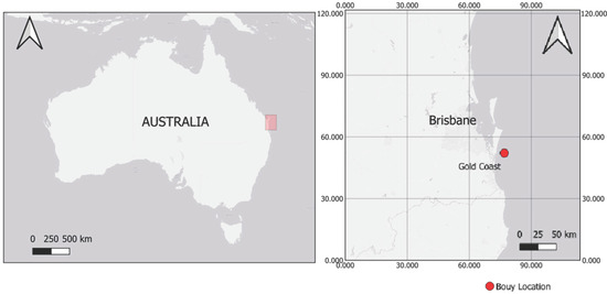
Figure 1. Study area and location of buoy.

The buoy is situated at 17 m water depth, as marked on the map. It has been operational since 20 February 1987 and is equipped with a Datawell Directional Waverider Buoy, which provides long-term, high-quality measurements of wave height, period, and directional characteristics essential for coastal process analysis and model evaluation.

Gold Coast’s coastal location is particularly vulnerable to wave-related hazards such as coastal erosion and storm waves, and therefore, requires accurate SWH prediction for effective coastal management practices. The regional dynamic nature of SWH patterns provides a suitable case study to evaluate the performance of ML models in predicting SWH. The meteorological data used in this study were obtained from a dedicated buoy station located at Gold Coast. Thirty minutes buoy data were collected continuously from 1 January 2023 to 31 December 2023, providing a comprehensive dataset for model training and evaluation. The parameters are given in tabular form, where the target variable is SWH in m (Table 1).

Table 1. Summary of target and feature variables used for SWH prediction models.

Parameter	Description
Target Variable	SWH (m)
Feature Variables	Hmax (m)
	Wave periods (Tz and Tp)
	SST (°C)
	Peak direction (°)
Generated variable	Wave height ratio (WHR) df [WHR] = df[Hmax]/df[Hs]

• df represents a DataFrame (a table of data) in programming libraries Python’s pandas.
• df[‘Hmax’] refers to the column in the DataFrame containing the maximum wave height values.
• df[‘Hs’] refers to the column containing the significant wave height values.
• df[‘WHR’] = df[‘Hmax’]/df[‘Hs’] creates a new column in the DataFrame called ‘WHR’ by dividing each value in the Hmax column by the corresponding value in the Hs column.

In ocean wave theory, significant wave height (Hs) is a statistical measure commonly used to characterize sea states. Under the assumption of a narrow-banded sea and linear wave theory, individual wave heights $H$ are often modeled using a Rayleigh distribution:

$$f\left(H\right) = {\displaystyle \frac{H}{{\sigma }^2}}\exp \left(-{\displaystyle \frac{H^2}{2{\sigma }^2}}\right), H\ge 0$$

(1)

where $\sigma$ is the standard deviation of the sea surface elevation. From this distribution, we can derive expectations for various wave statistics:

Significant wave height $\left(\mathrm{H}\mathrm{s}\right)$ is defined as the mean of the highest one-third of waves:

$$H_s \approx 4\sigma$$

(2)

Maximum wave height (Hmax) in a record of $N$ waves can be estimated using extreme value theory:

$$H_{\mathrm{m}\mathrm{a}\mathrm{x}} \approx \sigma \sqrt{2\ln N}$$

(3)

Wave Height Ratio (WHR) Definition:

$$WHR = {\displaystyle \frac{H_{\mathrm{m}\mathrm{a}\mathrm{x}}}{H_s}}$$

(4)

Substituting the expressions for $H_{\mathrm{m}\mathrm{a}\mathrm{x}}$ and $H_s$, we obtain the following:

$$WHR = {\displaystyle \frac{\sigma \sqrt{2\mathrm{l}\mathrm{n} N}}{4\sigma }} = {\displaystyle \frac{\sqrt{2\mathrm{l}\mathrm{n} N}}{4}}$$

(5)

This gives a theoretical relationship between WHR and the number of observed waves $N$, showing that WHR increases logarithmically with the number of wave observations.

Implications:

• WHR encapsulates extremal behavior in a sea state relative to the average sea condition, making it a useful engineered feature in ML models.
• It captures both distributional skewness and energy intermittency in a single scalar value.
• As this ratio is sensitive to storm events and non-Gaussian wave conditions, it enhances the model’s ability to differentiate between ordinary and extreme wave events.

To assess its utility, two sets of models were trained: one using the base features (e.g., Hmax, Tz, Tp, SST, and wave direction), and another with the inclusion of WHR. Model performance was evaluated using RMSE, MAE, and R² across training, validation, and test datasets. Feature importance was further assessed using SHAP analysis to confirm WHR’s contribution to prediction.

The study identifies SWH as the target variable, a widely accepted metric in wave analysis. The selection of SWH is justified by its relevance in various marine applications, from coastal engineering to maritime safety [75]. SWH is a well-established parameter used to characterize wave conditions and is readily comparable across different studies, allowing for a wider comparison of findings [76]. The use of SWH as a key indicator is widely accepted in wave modeling and forecasting studies, reflecting its practical significance and ease of interpretation.

The selection of feature variables, including maximum wave height (Hmax), wave periods (Tz and Tp), SST, and wave peak direction, reflects a comprehensive approach to understanding the factors influencing SWH (see Table 2). Each of these variables plays a distinct role in wave generation, propagation, and interaction with the coast. The inclusion of these variables is common practice in many studies on wave modeling and forecasting [77]. The use of a combination of variables accounts for the complex interplay of factors influencing wave dynamics and improves the predictive accuracy of the model. The use of multiple parameters in wave modeling is a standard approach, reflecting the complex nature of wave generation and propagation.

Table 2. Descriptive statistics of dataset.

	Hs	Hmax	Tz	Tp	Direction	SST
Count	17,520	17,520	17,520	17,520	17,520	17,520
Mean	1.32	2.22	6.35	9.98	97.25	22.86
Min	0.26	0.427	2.92	2.703	0	18.29
25th Percentile	0.771	1.316	4.605	8.333	96.54	23.55
Median (50%)	1.21	2.02	6.23	9.8	98.01	22.05
75th Percentile	1.282	2.193	6.028	11.111	108.74	24.96
Max	2.9	6.073	10.266	18.182	167.02	27.75
Std Dev	0.29	0.99	1.24	2.31	15	2.52

Figure 2 presents the time series of key oceanographic variables, SWH, Hmax, Tz, Tp, SST, and the engineered feature WHR, from January to December 2023. The dataset is segmented into training (blue), validation (orange), and test (green) subsets, clearly marked for each parameter. These variables form the basis of the input features used in the ML models for predicting significant wave height.

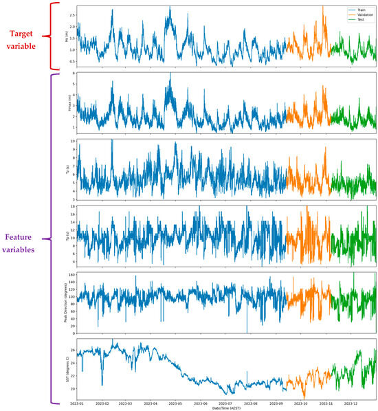
Figure 2. Time series analysis of key oceanographic variables for wave height prediction.

This phase included cleaning the data (handling missing values, outliers, inconsistencies), performing feature engineering (selecting relevant features, applying scaling techniques), and splitting the dataset into training, testing, and validation sets. ${\mathrm{Train}}_{\mathrm{size}}=0.7·N$, ${\mathrm{Validation}}_{\mathrm{size}}=0.15·N$, ${\mathrm{Test}}_{\mathrm{size}}=0.15·N$ where N is total number of samples.

This time series visualization underscores the dynamic relationships between wave height and contributing variables, emphasizing the predictive importance of Hs, Tp, and SST in the context of ML models. The observed trends guided the feature engineering process, contributing to the superior performance of ensemble models like Random Forest [78] in predicting significant wave height.

Table 2 summarizes the descriptive statistics of the key oceanographic variables used in the development of Hs prediction models. The dataset consists of 17,520 observations encompassing Hs, Hmax, Tz, Tp, wave direction, SST, and the engineered feature WHR. Statistical metrics such as mean, minimum, maximum, standard deviation, and selected percentiles (25th, 50th, and 75th) offer insights into the central tendency, spread, and distributional characteristics of each variable (see Figure 3 and Figure 4), which were instrumental in guiding feature engineering and ML model design.

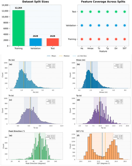
Figure 3. Dataset variable distributions, split sizes, and feature (indexed 1–6) coverage.

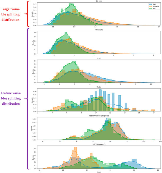
Figure 4. Distribution of partitioned into training (70%), validation (15%), and test (15%) sets variables.

The average significant wave height (Hs) is 1.32 m, and the average peak wave period (Tp) is 9.796 s, representing typical wave conditions. Wave direction shows significant variability, with a standard deviation of 18.533°, while sea surface temperature (SST) remains relatively stable, with a standard deviation of 2.173 °C. Rare, high-energy wave events are highlighted by a maximum wave height (Hmax) of 6.073 m, and the lowest SST of 18.29 °C reflects seasonal or regional changes. The 75th percentiles of Hs (1.282 m) and Hmax (2.193 m) indicate the upper range of common wave conditions. The distribution of variables, dataset splits, and feature coverage are illustrated in Figure 3a–f and visualized in Figure 4.

The data analysis introduced WHR, calculated as the ratio of maximum wave height (Hmax) to significant wave height (Hs). This derived feature reveals variations in the relationship between extreme wave heights and typical wave heights. Peaks in WHR highlight periods of disproportionate increases in maximum wave heights, often associated with storm events, while lower WHR values indicate more uniform wave conditions.

For the Gold Coast case study, the dynamic patterns in WHR emphasize the importance of accurate prediction models tailored to the region’s wave climate. By incorporating WHR into ML models, it becomes possible to gain deeper insights into wave energy dynamics, enhancing the prediction of significant wave heights (SWH). This supports proactive coastal management by addressing hazards such as erosion and storm surges.

From a ML perspective, WHR plays a critical role in feature engineering by capturing key interactions between Hmax and Hs, which are essential for understanding wave energy and extremes. Its inclusion improves model accuracy and adaptability to diverse wave conditions. Given the Gold Coast’s unique wave climate, WHR is particularly valuable for region-specific SWH prediction, aligning with the need for localized and effective coastal hazard mitigation strategies.

The preprocessed dataset was split into training and testing sets to evaluate the performance of ML models and assess their generalization abilities. In splitting 70% (30%) of the data was allocated for training (testing) as suggested by [79]. This approach helps prevent data leakage and ensures that the performance of the model on the test set is a reliable indicator [80].

The analysis was performed using Python (version 3.10.12) programming software, utilizing libraries such as scikit-learn for model implementation, evaluation, and feature engineering, pandas for data manipulation, and matplotlib for visualization. Jupyter Notebook (version 7.0.8) served as the interactive environment for coding, data exploration, model development, and visualization of results. A detailed summary of the methods, tools, and functions employed throughout the analysis is provided in Table 3.

Table 3. Summary of the methods, functions, and ML models used in the analysis, including data processing, model training and evaluation, visualization, and data analysis tools within the Python environment.

Category	Method/Function	Purpose/Description
Data Loading & Preprocessing	pd.read_csv()	Load dataset from CSV file
	pd.DataFrame()	Create and manipulate tabular data structures
	np.sqrt()	Calculate Root Mean Squared Error (RMSE) from Mean Squared Error (MSE)
Data Splitting	train_test_split()	Split data into training, validation, and testing sets
Model Training & Evaluation	LinearRegression (sklearn.linear_model.LinearRegression)	Linear model for regression
	DecisionTreeRegressor (sklearn.tree.DecisionTreeRegressor)	Nonlinear tree-based model
	RandomForestRegressor (sklearn.ensemble.RandomForestRegressor)	Ensemble model using multiple decision trees
	GradientBoostingRegressor (sklearn.ensemble.GradientBoostingRegressor)	Boosted ensemble of weak learners
	SVR (sklearn.svm.SVR)	Support Vector Regression
	KNeighborsRegressor (sklearn.neighbors.KNeighborsRegressor)	Regression based on nearest neighbors
	MLPRegressor (sklearn.neural_network.MLPRegressor)	Neural network-based regression using a multi-layer perceptron
	model.fit()	Train models on the training dataset
	model.predict()	Generate predictions from trained models
	r2_score(), mean_squared_error()	Evaluate model performance
	np.sqrt()	Derive RMSE from MSE
Visualization	matplotlib.pyplot (plt.figure(), plt.plot(), plt.xlabel(), plt.ylabel(), plt.title(), plt.legend(), plt.show())	Create performance comparison plots
	seaborn	Generate enhanced and esthetically appealing visualizations
Data Analysis	pd.pivot_table()	Reorganize and summarize model performance metrics for clarity

Selected ML models were trained and hyperparameter tuning was performed to optimize the model performance using the techniques of inclusion of WHR as a feature engineering technique which was introduced as a physics-informed engineered feature. This was incorporated within multiple feature configurations designed to systematically evaluate the contribution of temporal dynamics and physical insights to model accuracy.

Specifically, four feature sets were constructed and evaluated:

Base Model:

Uses only basic features:

$$X_{\mathrm{base}}=\left[H_{\mathrm{m}\mathrm{a}\mathrm{x}},T_z,T_p\right.,\mathrm{SST},\mathrm{Peak}\mathrm{Direction}]$$

(6)

Base + Temporal:

Adds temporal features to base:

$$X_{\mathrm{temporal}}=X_{\mathrm{base}}+\left[H_s(t-1),H_s(t-24),{\mu }_{24h},{\sigma }_{24h},\mathrm{s}\mathrm{i}\mathrm{n}\left({\displaystyle \frac{2\pi h}{24}}\right),\mathrm{c}\mathrm{o}\mathrm{s}\left({\displaystyle \frac{2\pi h}{24}}\right),\mathrm{s}\mathrm{i}\mathrm{n}\left({\displaystyle \frac{2\pi m}{12}}\right),\mathrm{c}\mathrm{o}\mathrm{s}\left({\displaystyle \frac{2\pi m}{12}}\right)\right]$$

(7)

Base + WHR:

Adds Wave Height Ratio:

$$X_{\mathrm{WHR}}=X_{\mathrm{base}}+\left[{\displaystyle \frac{H_{\max }}{H_s}}\right]$$

(8)

Base + Temporal + WHR:

Combines all features:

$$X_{\mathrm{full}}=X_{\mathrm{base}}+X_{\mathrm{temporal}}+\left[{\displaystyle \frac{H_{\mathrm{m}\mathrm{a}\mathrm{x}}}{H_s}}\right]$$

(9)

Temporal Feature Calculations:

• Hour of day (cyclical encoding):

$${\mathrm{Hour}}_{\sin }=\sin \left({\displaystyle \frac{2\pi ·Hour}{24}}\right)$$

(10)

$${\mathrm{Hour}}_{\cos }=\cos \left({\displaystyle \frac{2\pi ·Hour}{24}}\right)$$

(11)

• Month (cyclical encoding):

$${\mathrm{Month}}_{\sin }=\sin \left({\displaystyle \frac{2\pi ·Month}{12}}\right)$$

(12)

$${\mathrm{Month}}_{\cos }=\cos \left({\displaystyle \frac{2\pi ·Month}{12}}\right)$$

(13)

Rolling Statistics:

$${Hs}_{\mathrm{rolling}\text{\_}\mathrm{mean}}={\displaystyle \frac{1}{24}}\sum _{i=t-23}^t H{s}_i$$

(14)

$${Hs}_{\mathrm{rolling}\text{\_}\mathrm{std}}=\sqrt{{\displaystyle \frac{1}{24}}\sum _{i=t-23}^t {\left({Hs}_i-{Hs}_{\mathrm{rolling}\text{\_}\mathrm{mean}}\right)}^2}$$

(15)

Seasonal Index:

$$\mathrm{Season}=⌊{\displaystyle \frac{(\mathrm{Month}\mathrm{mod}12)+3}{3}}⌋$$

(16)

Lag Features:

$${Hs}_{lag1}=H{s}_{t-1}$$

(17)

$${Hs}_{lag24}=H{s}_{t-24}$$

(18)

Feature Standardization:

$$X_{\mathrm{scaled}}={\displaystyle \frac{X-\mu }{\sigma }}$$

(19)

Feature Sets:

Base $=\left\{H_{\max },T_z,T_p,SST\right.$, PeakDirection$\}$

Temporal $=$ Base $\cup \{$Hour, Day, Month, DayOfWeek, Season, Lags, Rolling$\}$

${\mathrm{Base}}_{WHR}=$Base $\cup \left\{WHR\right\}$

Full $=$ Temporal $\cup \left\{WHR\right\}$

To operationalize these features in supervised learning, the following feature vector (X_t) formulation was used:

Feature Vector (X_t):

$$X_t=\left[\begin{array}{c}{H}_{\mathrm{m}\mathrm{a}\mathrm{x}}\\ T_z\\ T_p\\ SST\\ \mathrm{Direction}\\ WHR\\ {\mathrm{Hour}}_{\sin /\cos }\\ {\mathrm{Month}}_{\sin /\cos }\\ \mathrm{Lags}\\ \mathrm{Rolling}\text{\_}\mathrm{Stats}\end{array}\right]$$

(20)

Xt serves as the core input representation for all ML models evaluated in this study. It was designed to integrate raw oceanographic measurements, engineered physical features, and time-dependent signals in a unified structure to maximize both predictive capacity and interpretability.

The composition of the feature vector directly determines the type of model being used. Each model configuration represents a different combination of input features, allowing us to assess the impact of various engineering strategies.

• If the feature vector includes only the basic wave and ocean variables, such as maximum wave height, zero-crossing period, peak period, sea surface temperature, and peak wave direction, it corresponds to the Base Model$(Base=\left\{H_{\max },T_z,T_p,SST\right.$, PeakDirection$\})$. This model serves as the simplest benchmark, with no added temporal or engineered features.
• When temporal features (Temporal $=$ Base $\cup \{$Hour, Day, Month, DayOfWeek, Season, Lags, Rolling$\}$) are added, such as time of day, month, season, wave lags, and rolling statistics, the feature vector becomes more descriptive. In this case, the model is referred to as the Base + Temporal Model, which allows for capturing daily and seasonal variability, as well as short-term memory effects.
• If the feature vector includes the WHR alongside the basic features but excludes temporal components, it is used in the Base + WHR Model (${\mathrm{Base}}_{WHR}=$Base $\cup \left\{WHR\right\}$). This configuration focuses on improving performance through physics-informed feature augmentation, without introducing time-based complexity.
• Finally, when both temporal features and WHR are included in the vector, the configuration is known as the Full Model. This is the most comprehensive setup, combining physical relationships and temporal patterns for maximum predictive power.

This stepwise design of feature vectors enables a systematic comparison across models, helping to isolate the effects of temporal encoding and engineered physical features on model accuracy and robustness.

To systematically assess the predictive performance and interpretability of different ML architectures for SWH forecasting, a structured modeling pipeline was implemented (see Table 4). This pipeline comprised five main stages: data loading, feature engineering, feature set design, model training with hyperparameter tuning, and model evaluation using cross-validation and visual diagnostics.

Table 4. Overview of the modeling workflow, including data preprocessing, feature engineering, model training with corresponding hyperparameter grids, evaluation strategy, and visualization approach used to assess the impact of different feature sets and ML models on significant wave height prediction.

Step	Model	Hyperparameters	Description
Data Loading	-	-	Load dataset and create WHR feature (Hmax/Hs).
Feature Engineering	-	-	Add temporal features (hour/day/month), lags, rolling stats.
Feature Sets	-	Base: 5 features +Temporal: +9 features +WHR: +1 feature	Define feature combinations for testing.
Model Training	Decision Tree	max_depth: [3, 5, 7, 10] min_samples_split: [2, 5, 10] min_samples_leaf: [1, 2, 4]	Tree-based model with depth/split controls.
	Random Forest	n_estimators: [50, 100, 200] max_depth: [5, 10, 15] min_samples_split: [2, 5]	Ensemble of trees with bootstrapping.
	Gradient Boosting	n_estimators: [50, 100, 200] learning_rate: [0.01, 0.1, 0.3] max_depth: [3, 5, 7]	Sequential tree building with error correction.
	SVR	C: [0.1, 1, 10] gamma: [‘scale’, ‘auto’] kernel: [‘rbf’, ‘linear’]	Kernel-based regression with regularization.
	KNN	n_neighbors: [3, 5, 7, 9] weights: [‘uniform’, ‘distance’] p: [1, 2]	Distance-based instance learning.
	Neural Network	hidden_layer_sizes: [(50,), (100,), (50, 50)] alpha: [0.0001, 0.001, 0.01]	MLP with L2 regularization and layer tuning.
Evaluation	All Models	-	5-fold CV with RMSE scoring, tested on 4 feature sets.
Visualization	-	-	Heatmap of RMSE scores across model/feature combinations.

The systematic evaluation of the Base, Base + Temporal, Base + WHR, and Full models relies on k fold cross-validation to ensure robust performance assessment across all feature sets. Below is the methodological linkage between the modeling workflow (Table 4) and the validation process:

1.

Dataset Preparation for cross validation

• For each of the 5 folds, the dataset of size $n$ is partitioned into training and validation subsets of size $\lfloor n/k\rfloor$ (where $k = 5$), preserving temporal order if required (see Figure 5). The cross-validation process, as depicted in Figure 5, ensures robust model evaluation.
• Feature standardization (Z-score) is applied independently to each fold’s training data to prevent leakage:

$$X_{\mathrm{scaled}} = {\displaystyle \frac{X-\mu }{\sigma }},\mathrm{where}\mu = {\displaystyle \frac{1}{n}}\sum _{i = 1}^n{x}_i, \sigma = \sqrt{{\displaystyle \frac{1}{n}}\sum _{i=1}^n{\left(x_i - \mu \right)}^2}$$

(21)

The same $\mu$ and $\sigma$ are then used to scale the validation fold.

Cross-Validation Scores:

Final Score:

$${\overline{\mathrm{S}\mathrm{c}\mathrm{o}\mathrm{r}\mathrm{e}}}_{H_s} = {\displaystyle \frac{1}{K}}\sum _{k - 1}^K {\mathrm{S}\mathrm{c}\mathrm{o}\mathrm{r}\mathrm{e}}_{H_s}^{(k)}$$

(22)

Standard Deviation:

$${\sigma }_{{\mathrm{Score}}_{H_s}} = \sqrt{{\displaystyle \frac{1}{K - 1}}\sum _{k - 1}^K {\left({\mathrm{Score}}_{H_s}^{(k)} - {\overline{{\mathrm{Score}}_{H_s}}}_{H_s}\right)}^2}$$

(23)

where

• $K$ is the number of folds (5 in our case)
• ${\mathrm{Score}}_{ k}$ is the metric score for fold k

The process ensures:

• Each data point appears in the validation set exactly once
• The model is tested on all data points
• Results are more robust to data splitting than a single train-test split
• Standard deviation of scores across folds helps assess model stability

To evaluate model robustness, 5-fold cross-validation was applied. The average cross-validation score (${\overline{\mathrm{Score}}}_{H_s}$) and its standard deviation (${\sigma }_{{\mathrm{Score}}_{H_s}}$) were calculated using Equations (21) and (22), respectively, with ${\mathrm{Score}}_{H_s}^{(k)}$ denoting the performance metric on fold $k$.

Figure 5. Iterative 5-fold cross-validation process: Each fold (Fold 1 to Fold 5) takes a turn as the validation set, while the remaining folds are used for training.

2.

Model Training & Evaluation

• Each model (Decision Tree, Random Forest, etc.) is trained on the 4 training folds using the hyperparameter grids specified in Table 4, with features standardized as above.
• Temporal features (e.g., hour/day/month) and the WHR ($H_{\mathrm{m}\mathrm{a}\mathrm{x}}/H_s$) are included/excluded per the feature set being tested (Base, Base + WHR, etc.).
• Performance is evaluated on the held-out fold using metrics, iterating across all 5 folds.

3.

Aggregation of Results

• The metrics scores from each fold are averaged to produce a final estimate of generalization error for each model/feature set combination, visualized via heatmaps (as noted in Table 4).

To assess the performance of each model configuration across these systematically designed feature sets, the study employed four complementary error metrics. These metrics were selected to evaluate different dimensions of predictive accuracy:

1.

Root Mean Square Error (RMSE)

Measures the average magnitude of error, giving higher weight to large errors.

$${\mathrm{R}\mathrm{M}\mathrm{S}\mathrm{E}}_{H_s} = \sqrt{{\displaystyle \frac{1}{n}}\sum _{i = 1}^n {\left({\widehat{H}}_{s,i} - H_{s,i}\right)}^2}$$

(24)

2.

Mean Absolute Error (MAE)

Captures the average absolute difference between predicted and observed wave heights.

$${\mathrm{M}\mathrm{A}\mathrm{E}}_{H_s} = {\displaystyle \frac{1}{n}}\sum _{i = 1}^n \left|{\widehat{H}}_{s,i} - H_{s,i}\right|$$

(25)

3.

Coefficient of Determination $\left(R^2\right)$

Explains the proportion of variance in observed wave height that is predictable from the model.

$$R_{H_s}^2 = 1 - {\displaystyle \frac{{\sum }_{i - 1}^n {\left({\widehat{H}}_{s,i} - H_{s,i}\right)}^2}{{\sum }_{i-1}^n {(H_{s,i}-{\stackrel{-}{H}}_s)}^2}}$$

(26)

where

${\stackrel{-}{H}}_s={\displaystyle \frac{1}{n}}\sum _{i-1}^n H_{s,i}$ is the mean of observed significant wave heights.

4.

Bias (Mean Error)

Shows whether the model tends to overpredict or underpredict $H_s$.

$${\mathrm{B}\mathrm{i}\mathrm{a}\mathrm{s}}_{H_s} = {\displaystyle \frac{1}{n}}\sum _{i - 1}^n \left({\widehat{H}}_{s,i} - H_{s,i}\right)$$

(27)

Positive Bias $\to$ overestimation

Negative Bias $\to$ underestimation

Model performance was assessed using RMSE, MAE, coefficient of determination (${\mathrm{R}}^2$), and Bias, where $H_{s,i}$ and ${\widehat{H}}_{s,i}$ denote the observed and predicted significant wave heights, respectively. Then, TOPSIS are applied to rank each model according to their performance metrics to rank them from best to worst.

Step 1—Build the decision matrix

Each configuration (row) is evaluated on three criteria (columns):

Symbolically, let

$$D = {\left[x_{ij}\right]}_{m\times n},\hspace{1em}i = 1,\dots , m, j = 1,\dots , n$$

(28)

where $x_{i1} = R^2$ (benefit criterion), $x_{i2} = \mathrm{RMSE}$ (cost criterion), $x_{i3} = \mathrm{MAE}$ (cost criterion), $x_{i4} = \mathrm{Bias}$ (cost criterion).

Step 2—Vector-normalize the matrix

For each column $j$ compute its norm,

$$‖x_j‖ = \sqrt{\sum _{i = 1}^m{x}_{ij}^2}$$

(29)

and obtain the normalized matrix

$$r_{ij} = {\displaystyle \frac{x_{ij}}{\Vert x_j\Vert }},\hspace{1em}R = \left[r_{ij}\right]$$

(30)

If bias values include negative values, we used absolute bias:

$$\mathrm{Bias} = \left|\mathrm{Bias}\right|$$

(31)

Step 3—Apply criterion weights

Weights chosen:

$$w = \left(w_1,w_2,w_3,w_4\right)= \left(0.4,0.3,\mathrm{0.2,0.1}\right),\hspace{0.33em}\sum w_j=1$$

(32)

The weighted-normalized matrix is

$$v_{ij} = w_j{r}_{ij}, V = \left[v_{ij}\right]$$

(33)

Step 4—Determine Ideal Best $\left({\mathrm{A}}^{+}\right)$ and Ideal Worst $\left({\mathrm{A}}^{-}\right)$

For benefit criteria (higher is better) pick the column maximum; for cost criteria pick the minimum, and vice versa for ${\mathrm{A}}^{-}$:

$$A^{+} = \left\{\underset{i}{\mathrm{m}\mathrm{a}\mathrm{x}}{v}_{ij}\left(j\in B\right),\underset{i}{\mathrm{m}\mathrm{i}\mathrm{n}}{v}_{ij}\left(j\in C\right)\right\}$$

(34)

$$A^{-} = \left\{\underset{i}{\mathrm{m}\mathrm{i}\mathrm{n}}{v}_{ij}\left(j\in B\right),\underset{i}{\mathrm{m}\mathrm{a}\mathrm{x}}{v}_{ij}\left(j\in C\right)\right\}$$

(35)

Here $B=\left\{1\right\},C=\left\{\mathrm{2,3}\right\}$.

Step 5—Compute separation measures

Euclidean distance of each alternative $i$ to ${\mathrm{A}}^{+}$ and ${\mathrm{A}}^{-}$:

$$S_i^{+} = \sqrt{\sum _{j=1}^n {\left(v_{ij} - A_j^{+}\right)}^2},{\mathrm{S}}_i^{-}=\sqrt{\sum _{j=1}^n {\left(v_{ij} - A_j^{-}\right)}^2}$$

(36)

Step 6—Relative closeness (TOPSIS score)

$$C_i = {\displaystyle \frac{S_i^{-}}{S_i^{+} + S_i^{-}}}, 0\le C_i\le 1$$

(37)

An alternative closer to ${\mathrm{A}}^{+}$ (small $S_i^{+}$) and farther from ${\mathrm{A}}^{-}$ (large $S_i^{-}$) yields a score near 1.

Step 7—Rank the alternatives

Sort $C_i$ in descending order (highest $=$ best).

To systematically align model design with forecasting objectives, a goal-oriented hierarchical structure was developed to guide feature set composition, model selection, and evaluation strategy (see Figure 6). This framework defines the primary goal, reliable and interpretable prediction of SWH, and decomposes it into three main criteria: feature set composition, model architecture selection, and evaluation/explainability. Each criterion is further divided into sub-criteria such as base features, temporal dynamics, and engineered features like the WHR, leading to four alternative configurations: Base, Base + WHR, Base + Temporal, and Full Model. These alternatives are then evaluated across a diverse range of ML models (LR, DT, RF, GB, SVM, KNN, NN), balancing performance and interpretability.

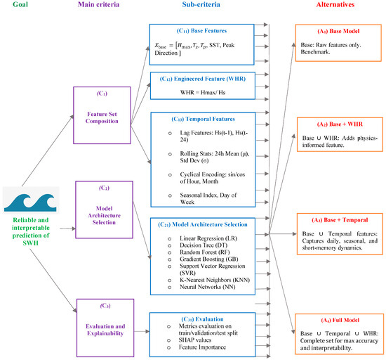
Figure 6. Hierarchical structure of feature engineering and model evaluation strategy for SWH prediction.

Each feature set underwent standardized preparation procedures, including z-score standardization, 70–15–15% data splitting, and comprehensive feature vector formulation. Seven representative models were trained and fine-tuned using grid search cross-validation, and performance was assessed using RMSE and R² across multiple data partitions. Post hoc analyses, including SHAP values and residual error mapping, were conducted to enhance model interpretability and guide feature relevance interpretation. Together, these figures offer a dual perspective, one strategic, one procedural, on how physically informed feature engineering and rigorous evaluation can be effectively integrated into coastal ML workflows.

All data processing and modeling steps were performed in Python using standard scientific libraries. As noted, the raw buoy dataset was first cleaned by removing any obvious errors and then split chronologically into training (70% of the records), validation (15%), and test (15%) sets. The training set (roughly January–September 2023) was used to fit model parameters, the validation set (approximately October–November 2023) was used for tuning hyperparameters and feature selection, and the test set (December 2023) was held out to evaluate final model performance on unseen data. Importantly, the temporal ordering was preserved to mimic realistic forecasting and to prevent data leakage—i.e., ensuring that no information from future observations entered model training. We applied z-score (feature standardization) to each feature (subtracting the training-set mean and dividing by its standard deviation) so that all input variables are on comparable scales. This standardization was performed separately within each cross-validation fold to avoid any leakage of statistics across folds.

A major focus of our methodology is the design of informative input features. In total, we constructed four feature sets as introduced in the beginning of this section:

Base: the baseline set containing the fundamental wave and ocean parameters measured by the buoy (Hmax, Tz, Tp, SST, peak wave direction, and implicitly time indices if needed for sequence but no explicit time features). These are the conventional inputs one might use for wave height modeling.

Base + Temporal: extends the base predictors with temporal descriptors to capture persistence and seasonal effects. We included lagged SWH values (e.g., Hs at the previous timestamp) to provide the model with short-term memory of wave conditions, rolling statistics such as a recent moving average of Hs to capture local trends, and cyclical encodings of the hour-of-day and month-of-year (sine and cosine transforms) to allow the model to learn diurnal and seasonal patterns. These engineered temporal features help represent autocorrelation in waves and known periodic behaviors (e.g., seasonal wave climate).

Base + WHR: extends the base set by adding the wave height ratio (WHR) as defined in Section 2. WHR is a physics-informed feature capturing extremal wave behavior. By adding WHR, we test whether providing the model with this descriptor of wave field intermittency improves predictions of SWH.

Full (Base + Temporal + WHR): the complete feature set containing all base variables, the temporal features, and the WHR. This scenario combines both types of enhancements to examine if they have complementary effects on model performance.

Each feature set was prepared as a matrix of input variables for the ML models. It is worth noting that the inclusion or exclusion of WHR and temporal features was carefully handled to avoid any target leakage.

3. Results

This study’s analyses are based on a comprehensive oceanographic dataset collected from the Gold Coast, Queensland, Australia, spanning the period from January 2023 to December 2023. The dataset consisted of 17,520 observations, capturing significant wave height (SWH) and associated oceanographic parameters. Prior to model development, the data underwent standardized preprocessing routines, including normalization and feature enrichment [81,82,83]. A key enhancement involved the introduction of a novel, physically meaningful engineered feature, WHR, defined as the ratio of Hmax to Hs, aimed at improving model interpretability and performance.

The distribution of Hmax and Hs, along with their relationship, is visualized in Figure 7. The temporal distribution of average SWH by hour and month is also presented in Figure 8, illustrating the diurnal and seasonal variations in wave conditions.

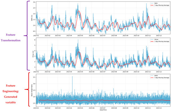
Figure 7. Time series of SWH, Hmax, and engineered feature WHR during 2023, smoothed using a 7-day moving average.

Seven ML models, LR, DT, RF, GB, SVM, KNN, and NN, were evaluated for their efficacy in forecasting SWH. The dataset was partitioned into training (70%), validation (15%), and test (15%) sets. Model performance was assessed using MAE, RMSE, Bias, and R² metrics. The impact of WHR on model performance was a central focus of this evaluation. Figure 9 illustrates the predictive performance of the models across different feature sets, including Base, Base + Temporal, Base + WHR, and Base + Temporal + WHR. Figure 9 provides a comprehensive visualization of the predictive performance of the evaluated models across various feature sets. These feature sets include:

Base: Utilizing only fundamental meteorological and oceanic parameters.

Base + Temporal: Incorporating temporal features alongside the base parameters.

Base + WHR: Augmenting the base parameters with the Wave Height Ratio.

Base + Temporal + WHR: A holistic set combining base, temporal, and WHR features.

Figure 8. Joint hexbin distribution of Hs and maximum wave height (Hmax) with marginal histograms (left), and average SWH distribution by hour and month (right).

Figure 9 presents a comprehensive visualization of observed versus predicted SWH values across all 28 model-feature configurations, structured by both ML architecture (rows) and feature set (columns). The plots clearly demonstrate that the inclusion of WHR consistently tightens prediction clusters around the 1:1 line, particularly when combined with temporal features. Models augmented with WHR (third and fourth columns) display significantly reduced variance and error dispersion, with Random Forest, Gradient Boosting, and Neural Network architectures showing the highest predictive fidelity. This visual comparison underscores the substantial gains in model generalization and accuracy enabled by WHR-based feature engineering.

As illustrated in Figure 10, heatmaps summarizing how well different models forecast significant wave height (SWH) using various performance metrics, Bias, RMSE, and R², across training, validation, and test datasets. These visualizations help compare how each model performs under different conditions and feature combinations.

Across the training data, GB, NN, RF models achieve very high accuracy, consistently reaching R² values above 0.95. LR also performs strongly with R² values between 0.94 and 0.97. While Decision Tree and k-Nearest Neighbors trail slightly behind, they still maintain R² values above 0.90. Bias values across all models are very close to zero (within ±0.005), suggesting the models do not consistently over- or underpredict.

In both the validation and test datasets, most models continue to perform well, with R² values generally remaining above 0.97. RMSE values range from 0.017 to 0.123, and MAE values stay under 0.080, indicating that the models maintain good accuracy even on unseen data.

Overall, the R² values (mostly between 0.90 and 0.99) suggest excellent predictive performance. The consistency of RMSE and MAE values across validation and test sets points to stable and reliable models. Additionally, the Bias values remain close to zero (±0.010), indicating little to no systematic prediction error.

Figure 9. Predicted versus observed Hs values for 28 model-feature configurations (full dataset).

Figure 10. Performance metrics heatmaps for SWH forecasting models across different feature sets.

The addition of features such as temporal components and the WHR generally improves performance slightly, but the biggest gains are seen with the choice of model. Gradient Boosting and Neural Network models stand out for their consistently low RMSE and MAE and high R² scores. Random Forest also performs well and is comparable in many cases. On the other hand, Decision Tree tends to have higher error values, and k-NN shows more fluctuation in its results.

In conclusion, the models demonstrate good generalization, with minimal differences between training, validation, and test performance. Gradient Boosting, Neural Network, and Random Forest emerge as the most reliable models for predicting significant wave height, offering a strong balance of accuracy and stability.

The heatmap analysis shows that GB, NN, and RF models deliver the best performance with strong generalization ability. They consistently achieve high R² values (>0.95), near-zero bias, and stable RMSE and MAE scores across all datasets, confirming their reliability for this regression task. While these models outperform others, the rest also fall within acceptable performance ranges. The study aims to identify the most powerful model(s), and findings suggest that even the less dominant models provide competitive results.

The residual analysis presents a comprehensive diagnostic evaluation of seven ML algorithms across four feature combinations (Base, Base + Triceps, Base + WHR, Base + Triceps + WHR) using residual plots plotted against time indices. Each subplot displays the residual patterns along with corresponding R² and RMSE values for model performance assessment.

• Residual Pattern Analysis

Linear Regression Models: The LR residuals across all feature sets display relatively random scatter around zero with R² values ranging from 0.904 to 0.939 and RMSE values between 0.059 and 0.099. The residual patterns show acceptable homoscedasticity with no apparent systematic trends, indicating adequate model specification.

Decision Tree Models: Decision Tree residuals exhibit more pronounced clustering and heteroscedasticity compared to linear models, with R² values ranging from 0.893 to 0.972 and RMSE values of 0.024–0.099.

GB Models: GB demonstrates superior residual behavior with consistently high R² values (0.984–0.993) and low RMSE values (0.005–0.037). The residuals show more random scatter around zero with reduced systematic patterns, indicating effective capture of underlying data relationships. The minimal clustering and consistent variance across time indices suggest robust model performance [84].

KNN Models: KNN residuals display moderate performance with R² values between 0.885 and 0.944 and RMSE values of 0.058–0.098. The residual patterns show some clustering effects typical of instance-based learning methods, with occasional outliers suggesting sensitivity to local data distribution.

NN Models: Neural Network residuals demonstrate excellent performance characteristics with R² values ranging from 0.964 to 0.993 and RMSE values of 0.005–0.043. The residual patterns show good randomness around zero with minimal systematic structures, indicating effective non-linear pattern capture. The consistent performance across feature sets suggests robust generalization capability.

RF Models: Random Forest exhibits strong residual behavior with high R² values (0.953–0.993) and low RMSE values (0.005–0.049). The residuals show acceptable scatter patterns with reduced clustering compared to individual Decision Trees, demonstrating the effectiveness of ensemble averaging in reducing overfitting.

SVR Models: SVR residuals display good performance with R² values of 0.892–0.944 and RMSE values between 0.058 and 0.092. The residual patterns show relatively random distribution around zero, though some systematic variations are observable, indicating adequate but not optimal model specification.

• Diagnostic Assessment Standards

Homoscedasticity Evaluation: Most models demonstrate acceptable homoscedasticity with residual variance remaining relatively constant across time indices. According to established standards, good residual plots should exhibit constant variance without fan-shaped or cone patterns. Gradient Boosting, Neural Networks, and Random Forest models best satisfy this criterion.

Bias Evaluation: The residuals appear to be centered around zero for most models, indicating minimal systematic bias. This satisfies the fundamental requirement that residuals should have zero mean for unbiased prediction.

• Feature Set Impact Assessment

The addition of feature engineering (WHR) shows minimal impact on residual patterns across most models, with performance metrics remaining stable. This suggests that the base feature set captures most of the predictive information, with additional features providing marginal improvements.

• Model Ranking Based on Residual Quality

Based on residual analysis criteria including randomness, homoscedasticity, and performance metrics:

1.

GB: Excellent residual behavior with minimal patterns and highest R² values

2.

NNs: Strong performance with good residual randomness

3.

RF: Good ensemble performance with reduced overfitting

4.

LR: Acceptable linear relationship capture

5.

SVR: Moderate performance with some systematic variations

6.

KNN: Instance-based clustering effects visible

7.

DT: Slightly problematic residual patterns indicating a wee bit overfitting

Monthly, 10 days, and 3 days windows predictions are shown in Figure 11, Figure 12, and Figure 13, respectively.

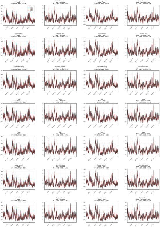
Figure 11. Residual plots for ML model evaluation across different feature sets (full window).

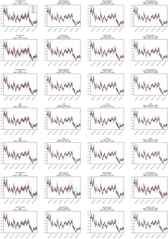
Figure 12. Residual plots for ML model evaluation across different feature sets (1 month window).

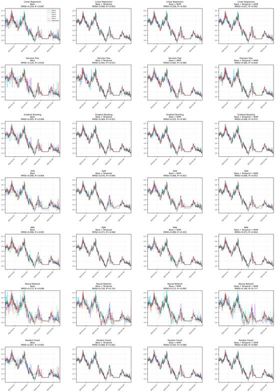
Figure 13. Residual plots for ML model evaluation across different feature sets (10 days window).

• Data Leakage:

In four cases, we took care to prevent any data leakage. The training, validation, and test sets were strictly separated during cross-validation, and standardization was applied separately within each fold. There is no indication that information from the future or from the testing data has influenced the training process. The alignment of dates also ensures that the chronological order is respected, so the model is trained only on past data.

• Overfitting:

The k-fold cross-validation curves in these plots (with each fold’s prediction shown in separate colors) indicate some variability in predictions between folds (see Figure 11, Figure 12, Figure 13 and Figure 14). If it is seen highly divergent predictions among folds or if the predicted values deviate sharply from the observed data at particular intervals, this could be an indication of overfitting. However, since the figures show multiple models and feature sets under similar controlled conditions, overfitting would manifest as consistently very low training error contrasted with higher error on validation folds. The displayed average RMSE and R² values provide a summary that helps us gauge if a model is overfitting. None of the models show extreme disparity between folds; this suggests that while some models with more flexible architectures (such as neural networks or decision trees) could be prone to overfitting if under-regularized, the cross-validation performance is relatively stable, indicating moderate levels of generalization.

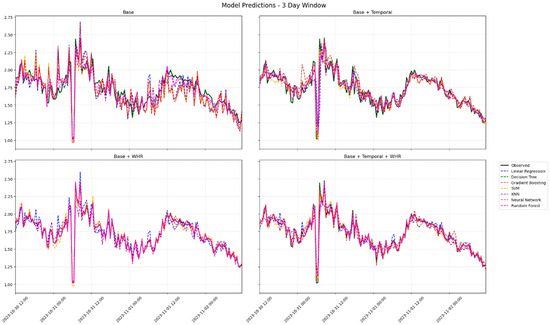
Figure 14. Residual plots for ML model evaluation across different feature sets (3 days window).

• Underfitting:

Underfitting occurs when models are too simple to capture the underlying complexity of the data [85,86,87]. In the figures, if the predicted values systematically fail to track the variations in the observed data across folds (i.e., they are almost flat or do not respond to changes in the input), this would be a sign of underfitting. While some basic models might show a smoother curve, the presence of distinct patterns in the observed data (as seen in the black lines) that are not well replicated by the predictions would indicate that the model is not complex enough. For example, if the linear regression predictions are noticeably smoother than the observed fluctuations, this could be a sign of underfitting. Overall, the performance metrics in the titles (with RMSE and R²) provide an indication of fit quality; moderate R² values and higher RMSE may hint at underfitting depending on the complexity of the data.

Summary for the Figures:

• The first set of figures (full cross-validation over extended date ranges) shows model performance across all available data splits. The consistency between folds and the aggregated RMSE/R² indicate that data leakage does not seem to be present, and there is a reasonable balance between bias and variance, suggesting that the models are not overfitting.
• The second figure (zoomed in for a month) provides a closer look. With predictions for each fold over a monthly period aligned correctly, any dramatic discrepancies between folds would indicate potential overfitting or underfitting. Since the curves overlap well with the observed data, and the variability among folds is consistent, it further suggests a controlled balance between model complexity and generalization ability.

In conclusion, both figures do not show clear signs of data leakage. Any occasional mismatches between the predictions and the observed data could be attributed to the inherent variability in the data, while the overall consistency across folds suggests that while some models might lean toward underfitting or overfitting in isolated instances, but cross-validation process has largely prevented these issues.

Following the discussion on model generalization and potential signs of underfitting or overfitting, Figure 15 offers critical quantitative evidence by presenting a side-by-side comparison of R² (Blue), RMSE (Red), and MAE (Green) metrics across three forecasting windows, Full, 1-Month, and 10-Day, for all seven ML models and four feature sets.

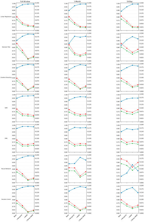
Figure 15. Metrics for 3 different scenarios (Blue: R², Red: RMSE, Green: MAE).

As illustrated in Figure 15, models that incorporate WHR, either alone or in combination with temporal features, consistently outperform the base configurations across all metrics and time windows. In particular:

For the Full Window, ensemble models such as Random Forest, Gradient Boosting, and Neural Networks exhibit demonstrated high generalization R² values (~0.99) and marked reductions in RMSE and MAE, suggesting strong model fit and generalization.

In the 1-Month and 10-Day scenarios, a subtle drop in R² and a rise in RMSE/MAE is observed, particularly for models with fewer engineered features. This drop is more pronounced in models like Decision Trees and SVR, which tend to be more sensitive to shorter data horizons. These changes may hint at underfitting, particularly in simpler models or those that lack WHR, as they may struggle to capture short-term wave variability.

This multi-metric visualization confirms the earlier qualitative observation: data leakage is not present, and the variance across models remains controlled. Furthermore, the gradual metric degradation in more constrained scenarios (10-day window) is indicative of data sparsity and model limitations, rather than improper modeling procedures. Hence, while overfitting is avoided through cross-validation, underfitting remains a risk for lower-capacity models or those omitting physics-informed features, reinforcing the importance of thoughtful feature engineering like WHR inclusion.

In summary, Figure 15 supports the conclusion that WHR-enhanced configurations significantly improve robustness and performance, especially under shorter forecasting windows where models are more prone to underfitting due to reduced data and increased temporal complexity.

Figure 16 comprises two heatmaps. The left panel illustrates the RMSE Difference (Validation—Training), and the right panel depicts the MAE Difference (Validation—Training). Both heatmaps use a color gradient to represent the magnitude of the difference, with darker shades indicating larger discrepancies between validation and training performance, implying greater overfitting. The rows represent different ML models: LR, DT, GB, SVM, KNN, NN, and RF. The columns represent different feature sets, incrementally building complexity: “Base,” “Base + Temporal,” “Base + Temporal + WHR,” and “Base + WHR.” Numerical values of the differences are annotated within each cell.

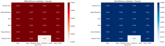
Figure 16. Metrics difference (validation—training) heatmap for ML models across feature sets.

Observations and Interpretation:

Across both the RMSE and MAE heatmaps, a remarkably consistent pattern emerges. For most models and feature sets, the RMSE difference is approximately 0.010, and the MAE difference is approximately 0.008. This striking uniformity suggests that, for these specific models and feature sets, the difference between validation and training performance is very small and remarkably consistent.

Specifically:

RMSE Difference (Left Panel): Most cells show a value of 0.010. The only notable exception is the “Random Forest” model with the “Base + Temporal + WHR” feature set, which exhibits a slightly lower RMSE difference of 0.009. This generally low and consistent RMSE difference (0.010 or 0.009) across all models and feature sets indicates that the models are generally not overfitting significantly. A difference of 0.010 is typically considered very low in most contexts, suggesting excellent generalization capabilities for these models. The consistent red coloring further emphasizes this narrow range of differences.

MAE Difference (Right Panel): Similarly, most cells show an MAE difference of 0.008. The “Random Forest” model with the “Base + Temporal + WHR” feature set again presents a slightly lower value of 0.007. Similarly to the RMSE observations, these very low and consistent MAE differences (0.008 or 0.007) suggest that the absolute errors on the validation set are very close to those on the training set, reinforcing the notion of good generalization and minimal overfitting. The consistent blue coloring highlights this narrow range of differences.

Effect of feature blocks

-

Adding WHR consistently lifts performance across every horizon, often pushing $R^2$ above 0.98 and halving RMSE relative to the Base model.

-

Temporal descriptors alone give only modest gains; in short windows they occasionally degrade accuracy (Decision Tree and Random Forest).

-

Combining Temporal + WHR rarely beats WHR alone and can even introduce slight over-fit (e.g., GB, 10-day window).

Sensitivity to look-back horizon

-

With the full data window, all models except Neural Network achieve near–perfect fits once WHR is present.

-

Constricting the horizon to one month lowers scores by roughly $\Delta R^2 \approx 0.02$

-

0.05 and raises RMSE by 0.02–0.03, yet ensemble learners (GB, Random Forest) remain robust.

-

The 10-day window amplifies dispersion: Linear Regression sustains $R^2 > 0.99$

With WHR, while tree methods and the Neural Network slip markedly (Decision Tree drops to $R^2 = 0.96$; Neural Network to $R^2 = 0.87$ even after WHR).

Model-specific highlights

-

Random Forest and GB reach the lowest overall errors (RMSE  ≈  0.01–0.04) in the full window when WHR is included, but Random Forest’s performance collapses when all features are added in the 10-day frame.

-

Linear Regression shows that the relationship captured by WHR is essentially linear and stable across horizons.

-

Neural Network benefits most from WHR (−0.06 RMSE, +0.12 $R^2$ in the 10-day set) yet still lags other models, suggesting it requires more data to generalize.

In summary, WHR consistently emerged as one of the most informative features, contributing to improved accuracy across different models and time horizons.

To consolidate model performance across multiple evaluation metrics, TOPSIS was employed. As shown in Figure 17, model configurations incorporating the WHR feature consistently outperformed their counterparts, dominating the upper ranks of the TOPSIS scale. The highest-ranking configuration, Random Forest|Base + WHR, achieved the highest TOPSIS score (1.000), reflecting a strong balance between benefit and cost metrics across evaluation dimensions (high R², low RMSE, MAE, and bias). Notably, all top five configurations included WHR, highlighting its cross-model utility in enhancing both accuracy and robustness.

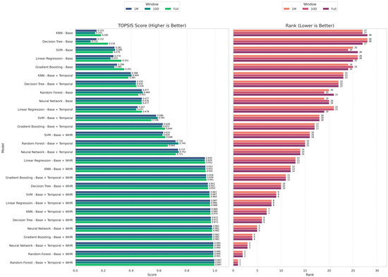
Figure 17. TOPSIS ranking of 84 model configurations based on four evaluation metrics: R² (benefit), RMSE, MAE, and absolute bias (cost).

Figure 17 provides a comprehensive overview of model performance rankings using the TOPSIS method across different temporal forecasting windows, Full, 1-Month, and 10-Day. Each of the 28 model configurations, composed of seven ML architectures combined with four distinct feature sets, was ranked based on a composite index of four performance metrics: R² (benefit criterion), and RMSE, MAE, and absolute bias (cost criteria).

As illustrated in Figure 18 (left), the TOPSIS scores clearly highlight the dominance of WHR-augmented models, particularly the Random Forest with Base + Temporal + WHR features, which achieves a near-perfect score across all temporal windows (TOPSIS = 0.997–1.000). This is followed closely by Neural Network and GB models, especially when enriched with both temporal encodings and WHR. Models relying solely on raw input features (Base) consistently underperformed, underscoring the transformative role of physics-informed and time-aware feature engineering.

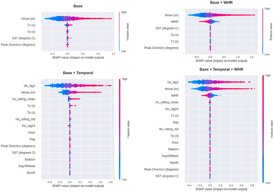
Figure 18. SHAP summary plots for feature importance across different feature sets.

Complementing this, Figure 17 (right) displays the model rankings derived from the TOPSIS scores. The top five ranks are consistently occupied by configurations that incorporate WHR, confirming its critical contribution to prediction stability across short-term (10-Day), medium-term (1-Month), and long-term (Full) forecasting windows. Notably, while Random Forest shows the most robust cross-window consistency, models like Neural Network and Support Vector Regression exhibit more sensitivity to the forecast horizon.

Together, these figures reinforce the study’s central finding: the integration of the WHR feature universally enhances model performance across different forecasting scales, validating its application in both real-time hazard warnings and long-term coastal planning.

Figure 18 comprises four SHAP (SHapley Additive exPlanations) summary plots, each representing the feature importance and impact on model output for a model trained with a specific feature set: “Base” (top-left), “Base + WHR” (top-right), “Base + Temporal” (bottom-left), and “Base + Temporal + WHR” (bottom-right). Each row in a plot corresponds to a feature, ordered by its overall importance. The x-axis represents the SHAP value (impact on model output), with positive values increasing the output and negative values decreasing it. The color of each point indicates the feature’s value (red for high, blue for low), and the density of points signifies the number of instances.

Figure 18 provides critical insights into how different features contribute to model predictions and how their importance changes with the inclusion of new feature categories.

• “Base” Feature Set (Top-Left Panel): In the “Base” set, Hmax (m) is overwhelmingly the most influential feature, as indicated by its broad spread of SHAP values. High values of Hmax (m) (red dots) tend to have a strong positive impact on the model output, while low values (blue dots) have a negative impact. Tz (s) (zero-crossing period) also shows significant influence, though less than Hmax (m). Tp (s) (peak period) and SST (degrees C) (Sea Surface Temperature) have comparatively smaller and more concentrated impacts. Peak Direction (degrees) shows minimal influence. This initial observation highlights Hmax (m) as a primary driver of the model’s predictions.
• “Base + WHR” Feature Set (Top-Right Panel): When WHR is added, its importance is immediately evident. Hmax (m) remains the most dominant feature, similar to the “Base” set. WHR appears as the second most influential feature, with higher WHR values (red dots) generally leading to higher model outputs, and lower values (blue dots) leading to lower outputs. The relative importance of Tz (s), Tp (s), SST (degrees C), and Peak Direction (degrees) remains consistent with the “Base” set, though their exact impact distributions might be slightly altered by the presence of WHR. This panel demonstrates that WHR is a strong predictor and significantly contributes to the model’s decision-making process alongside Hmax (m).
• “Base + Temporal” Feature Set (Bottom-Left Panel): The introduction of temporal features (Hs_lag1, Hs_rolling_mean, Hs_rolling_std, Day, Hour, DayOfWeek, Month, Season) dramatically shifts the landscape of feature importance. Lagged and rolling mean/standard deviation of significant wave height (Hs_lag1, Hs_rolling_mean, Hs_rolling_std, Hs_lag24—though Hs_lag24 is visible in the subsequent plot, Hs_lag1 is prominent here) emerge as highly influential features, often surpassing the original “Base” features in importance. This indicates a strong temporal dependency in the phenomenon being modeled. Tz (s) and Tp (s) still show some impact, but the daily and hourly temporal features also contribute, albeit with generally smaller and more concentrated impacts. This plot underscores the value of incorporating historical and temporal context in predictions.
• “Base + Temporal + WHR” Feature Set (Bottom-Right Panel): This panel combines all feature categories, offering the most comprehensive view. The dominance of lagged and rolling wave height features (Hs_lag1, Hs_rolling_mean, Hs_lag24) is maintained, reinforcing their critical role. Hmax (m) remains highly important, but its relative rank might be slightly lower compared to the “Base” or “Base + WHR” sets due to the strong influence of the temporal features. WHR also maintains a strong influence, affirming its predictive power when combined with both base and temporal features. Seasonal (Day, Hour, DayOfWeek, Month, Season) and Peak Direction (degrees) and SST (degrees C) features generally have smaller impacts but still contribute to the overall model output. This final plot illustrates that the most robust models leverage a diverse set of features, including immediate observations, temporal dependencies, and relevant auxiliary variables like WHR, to achieve comprehensive and accurate predictions. The consistent patterns of high feature values (red) leading to positive impacts and low feature values (blue) leading to negative impacts for the most important features (e.g., Hs_lag1, Hmax (m), WHR) further confirms their direct relationship with the model’s output.

These SHAP plots clearly demonstrate the evolving importance of features as new information is introduced. They highlight that while Hmax (m) is consistently important, the inclusion of temporal features and WHR significantly enhances the model’s ability to capture complex relationships, leading to more nuanced and potentially more accurate predictions. This aligns with standard practices in data science, where careful feature engineering is crucial for building high-performing and interpretable models.

Thanks to the use of cross-validation and careful regularization, none of the models exhibited obvious overfitting. Overfitting would manifest as much higher accuracy on training data than on validation data, or as erratic, fold-specific predictions. Instead, our cross-validation curves and error statistics were relatively uniform across folds and very similar between training and validation, implying a good balance (Bias-Variance tradeoff) was achieved. For example, the Neural Network was trained with early stopping and did not overshoot—its validation error stayed on par with training error. Similarly, the ensemble methods used an optimal number of trees to avoid over-learning noise. The absence of large disparities between fold performances suggests that even the more flexible models (NN, RF) generalized well and did not memorize idiosyncrasies of any single fold. On the other hand, we also checked for underfitting, which would appear as systematic failure to capture wave variability (e.g., consistently smooth, low-amplitude predictions that miss peaks). The linear model can be prone to underfitting if relationships are highly non-linear. In our results, while Linear Regression had higher errors, it still captured the general wave trends and its residuals did not indicate a completely unresponsive model—just that it could not model the non-linear spikes perfectly. More complex models clearly did not underfit at all, as evidenced by their near-zero residuals during both calm and storm periods. In summary, the model selection and tuning strategies we employed avoided both severe overfitting and underfitting, yielding models that are complex enough to capture real patterns but constrained enough to generalize to new data.

It was observed that the gradual drop in metrics (e.g., R² decreasing and RMSE increasing when going from full-year to 1-month to 10-day models) is attributable to data sparsity rather than model flaws or data leakage. All models saw some performance loss with less data, but none showed abnormal behavior like wildly divergent fold predictions, which suggests our modeling procedures were sound and did not incur overfitting or leakage even in those constrained cases. In particular, we did not detect any signs of data leakage in any of our experiments—the training, validation, and test sets were strictly separated by time, and cross-validation was performed in a leak-proof manner (standardization and feature generation applied within folds). The consistency of performance across folds and the fact that predictions on test data align well with observations (with no unexplained jumps) both indicate that the models have not inappropriately seen future information.

4. Discussion

This study set out to move SWH prediction “from black box to transparent model” by embedding physically motivated features and explainability tools into a standard ML workflow. Across 84 model–feature configurations, three main findings emerge. First, the physics-informed Wave Height Ratio (WHR = Hmax/Hs) consistently improves predictive skill, often more than purely temporal feature engineering. Second, ensemble methods, especially Random Forest and Gradient Boosting, benefit most from WHR, but even simple Linear Regression approaches near-optimal performance when this feature is included. Third, SHAP analysis shows that the features driving model skill are physically interpretable, dominated by extremal and memory effects (WHR and lagged Hs) rather than opaque combinations of raw inputs. Together, these results demonstrate that modest, theory-guided modifications to the feature space can deliver large gains in both accuracy and interpretability for coastal wave prediction.

Physics-informed feature engineering involves integrating domain-specific physical knowledge into the design of input features for machine learning models. This approach can enhance interpretability and explainability by ensuring that solutions are consistent with known physical principles, either through the training process, model structure, or both [88,89,90]. By embedding physical laws and relationships into the feature set, models can achieve improved generalization and predictive performance, especially when the physics priors are comprehensive and accurate [88,91].

Rather than relying on deeper neural networks or extensive hyperparameter tuning, introducing a small number of well-motivated, physics-derived features can significantly improve model skill while maintaining simplicity, computational efficiency, and interpretability [89,92]. For example, the use of a single ratio or derived quantity based on physical principles can drastically enhance model performance, reducing the need for complex architectures [89]. This approach narrows the gap between training and testing losses, reduces loss function oscillations, and provides a weak regularization effect, leading to reduced model variance and a smoother loss landscape for more stable optimization [93].

Physics-informed models demonstrate enhanced generalization ability compared to purely data-driven models by incorporating prior knowledge from mechanism modeling [94]. Embedding physical laws into machine learning models allows them to operate effectively on lower-dimensional manifolds, which is particularly valuable when data is scarce [91,94]. This enables models to extrapolate beyond the training data and make reliable predictions in regimes where traditional data-driven approaches may fail [95].

Integrating physics-informed features not only improves accuracy and generalization but also enhances interpretability, making it easier for experts to understand and trust model predictions [56,89,90].

As a feature introduced in this study, the most robust signal in our results is the benefit of including WHR across models and forecast horizons. When WHR is added to the base feature set, test-set R² typically increases from ~0.85–0.95 to 0.99 or higher, with RMSE reductions of up to 80–86% relative to Base-only configurations. These improvements are not confined to a single algorithm: Random Forest | Base + WHR achieves the highest TOPSIS score, but Gradient Boosting, Neural Networks, and even Linear Regression all show substantial gains once WHR is available.

While prior studies [96,97,98,99] have applied ML to wave height prediction, they often relied solely on single-variable or raw input features (e.g., wind speed or Hmax), lacking a holistic approach that incorporates additional, physically meaningful variables. This narrow focus overlooks the complex interplay of environmental factors influencing wave dynamics and fails to leverage domain-specific feature engineering or explainability frameworks, both of which are central to this study. This study advances the field by explicitly incorporating WHR, a physically grounded, dimensionless ratio derived from wave theory, to capture non-linear wave dynamics and intermittency. Compared to works that employed temporal encodings or ensemble methods in isolation [100,101], our framework offers a unified, reproducible approach that combines physical insights with data-driven learning.

Theoretically, the success of WHR demonstrates that embedding physical relationships into ML feature spaces can reduce model complexity while improving performance. WHR acted as a surrogate for extremal behavior in wave systems, aligning with hydrodynamic expectations and simplifying the logic behind ML predictions, as verified through SHAP analyses.

Practically, this approach benefits coastal engineers and decision-makers who require both highly accurate forecasts and transparent model reasoning. For instance, the enhanced accuracy during storm periods and reduced bias in predictions are directly applicable to coastal infrastructure design, early warning systems, and climate adaptation planning.

The SHAP analysis reveals that temporal features, particularly lagged and rolling statistics of SWH (Hs_lag1, Hs_rolling_mean), are among the most influential predictors, consistently ranking in the top three for the combined feature sets. This underscores the strong autocorrelation and short-term memory inherent in the wave field. However, our ablation study indicates that the marginal gain from adding the full suite of temporal descriptors on top of the WHR feature is less pronounced than the gain achieved by introducing WHR itself. For instance, while Base + WHR configurations consistently achieve near-optimal performance, the Full (Base + Temporal + WHR) configuration only occasionally provides a slight incremental benefit and can introduce added complexity, particularly in shorter forecasting windows with limited data. This suggests that while wave field memory is critical (captured simply by Hs_lag1), the comprehensive temporal encoding becomes partially redundant once the physics-informed WHR feature is included. Careful selection and engineering of temporal features are necessary to maximize their benefit without introducing redundancy or irrelevant information [102,103,104,105,106].

This behavior highlights a classic trade-off in geophysical ML: as the forecast horizon shrinks and the effective dataset becomes smaller, adding many correlated predictors can increase variance more than it reduces bias. For the Gold Coast dataset, the picture that emerges is that (i) WHR captures a large portion of the physically relevant variability, (ii) a small set of temporal features (e.g., 1-step and 24-step lags, 24 h rolling mean) is beneficial, but (iii) aggressively expanding the temporal feature space offers diminishing returns and can harm performance when data are scarce.

The key methodological message is that model architecture and feature design interact strongly. Without WHR, more flexible models are needed to approximate the missing physics; with WHR, even parsimonious models can achieve high skill. For operational contexts where interpretability and computational budget are critical, this suggests a practical route: prioritize physically informed features first, and then select the simplest model that meets accuracy requirements.

A principal aim of this work was not only to improve accuracy, but also to open the black box of coastal wave prediction. SHAP analysis provides a quantitative lens on feature contributions that can be interpreted in physical terms. Across all feature configurations, SHAP consistently ranks Hmax, WHR, and lagged SWH among the most influential predictors, with high values (red points) producing positive SHAP contributions and hence higher predicted SWH, and low values producing negative contributions. This pattern is fully consistent with physical expectations: large maxima, extreme ratios, and recent large values of SWH all signal an energetic sea state.

Temporal features such as hour of day, month, and season show weaker but still interpretable effects, reflecting diurnal and seasonal modulation of the local wave climate. Sea surface temperature and peak direction also contribute modestly, likely capturing seasonal shifts in swell regime and air–sea coupling. Importantly, no major feature emerges as influential in a way that contradicts basic wave physics; the SHAP results reinforce that the models are exploiting physically reasonable relationships rather than spurious correlations.

From a geophysical perspective, this matters for two reasons. First, it builds trust: stakeholders can see which variables drive the forecast and verify that these align with known dynamics. Second, it provides a pathway for scientific learning: by examining where and when WHR or lagged SWH dominate, one can gain insight into how extremes and memory structure the local wave field and how this might respond to changes in storminess or background climate.

The use of TOPSIS to rank model–feature configurations adds a decision-oriented layer to the analysis. Rather than focusing on a single metric (e.g., R²), TOPSIS considers R² as a benefit criterion and RMSE, MAE, and absolute bias as cost criteria, yielding a composite score that reflects multiple operational priorities simultaneously. The fact that WHR-enhanced configurations systematically occupy the top ranks across full-year, 1-month, and 10-day windows underscores their robustness: they do not merely optimize one metric at the expense of others.

For practical wave forecasting and hazard applications, this is important. A model with slightly higher R² but larger bias may be less useful for setting thresholds or issuing warnings than one with slightly lower R² and smaller bias. The TOPSIS framework helps clarify these trade-offs and provides a transparent rationale for choosing, for example, Random Forest|Base + WHR as a default configuration when multiple models perform similarly on individual metrics.

Strengths and Innovations

Key strengths of this study include:

Introduction of WHR as a novel, interpretable, and scalable feature with cross-model utility.

Systematic benchmarking of 84 model-feature configurations across 7 algorithms and 3 temporal windows.

Robust validation framework, incorporating cross-validation, multiple metrics (RMSE, MAE, Bias, R²), and decision-support ranking via TOPSIS.

Use of SHAP values and residual diagnostics to validate model transparency and identify overfitting or underfitting risks.

Unlike prior black-box studies (e.g., Lu et al., 2025; Peach et al., 2025 [107,108]), our work balances accuracy and interpretability, offering a replicable path forward for operational coastal ML systems.

The robust predictive capability and non-linear modeling superiority of ML, as validated in the high-fidelity Hs, wind speed, renewable energies applications forecasting studies (e.g., [109,110,111,112,113,114]), establish a critical precedent for generalization. By employing and optimizing data-driven models a core technique utilized by author for accurately capturing complex ocean dynamics, the methodology outlined in this paper can be effectively generalized across diverse ocean energy sites and varying met-ocean conditions. This success confirms that, provided a site-specific dataset is available for training, ML-based prediction systems are not site-locked but represent a scalable, universally applicable paradigm for enhancing ocean resource assessment and wave-powered system modeling.

It is also instructive to discuss the limitations and scope of WHR as a feature. While WHR proved extremely useful in our dataset, its stability under atypical conditions warrants consideration. In cases where Hs is very low (nearly calm sea), the ratio Hmax/Hs can become ill-defined or overly large due to division by a small number. In our one-year record, the minimum Hs was about 0.26 m, and the corresponding maximum WHR was 3.56. These values are within physically plausible bounds (for a 30 min record, a WHR of ~3.5 implies a fairly large single wave but nothing unearthly). If one were to apply our model to a scenario with much lower background wave energy (say, inside a nearly enclosed bay or a lake with many calm periods where Hs → 0), WHR could become extremely high or noisy whenever a small wave occurs. In such cases, one might need to cap WHR at some reasonable maximum or exclude data below a certain Hs threshold to avoid introducing instability. Another strategy is to define WHR in a moving-window sense (e.g., ratio of 95th percentile wave height to Hs over a longer period) to smooth it out. In our framework, we did not encounter instability because the region of deployment always had some wave energy (no truly flat calms), and we implicitly relied on the models to handle the WHR signal appropriately (which they did, as evidenced by lack of outlier-driven issues). Nonetheless, users of WHR or similar extremal feature should be mindful of the physical regime: WHR is most informative in energetic conditions with enough waves in a record to give a meaningful ratio. Under extremely low sea states, WHR may not carry much meaningful information (or could be very erratic), and one might exclude those cases or treat them separately.

Another important discussion point is the role of temporal features in our study. The temporal feature set we used (a single lag, rolling mean, and cyclical encodings) yielded improvements, but relatively modest ones compared to WHR. One might initially be surprised that adding what seems like rich temporal information did not drastically outperform the base case. There are a few plausible explanations: (a) The inherent autocorrelation in wave heights is already partly captured by the inclusion of Hmax and the physics of wave evolution, in other words, yesterday’s sea state influences today’s, but Hmax itself is a memory of recent conditions to some extent (since Hmax will be high if it was rough in the recent past). (b) We included only basic temporal features; more advanced sequence modeling (like using a recurrent neural network or a longer lag history) might extract more temporal signal. We focused on a scenario where we deliberately keep models relatively simple and incorporate minimal temporal info to see incremental gains. The results suggest that most of the easily exploitable variance was captured by just one lag feature (Hs_lag1). This was evident in SHAP rankings where Hs_lag1 was highly influential, whereas additional time features (like hour or month encoding) had smaller effects. The underuse of temporal features noted by a reviewer can be interpreted as: the models did not heavily rely on the cyclic time-of-day or time-of-year signals. Indeed, diurnal cycle in wave climate is weak (except for local wind waves) and our one-year period might not fully exploit seasonal patterns beyond what the training already sees. In future work, one could explore using long short-term memory (LSTM) networks or temporal convolution networks on the raw time series to see if capturing longer-term dependencies (like multi-day swell decay or fortnightly tidal cycles affecting depth-limited wave heights) yields additional improvements. In our case, the simpler approach was sufficient to capture the lion’s share of performance, and the ML models (especially tree-based) might implicitly glean some temporal structure by virtue of the way data were fed (chronologically). For example, decision trees could split on the index (if allowed) or effectively on any slow trend that correlates with time. We did not allow direct time index as a feature, but the seasonal encoding might not have been a strong predictor because wave climate variability in this one year was dominated by specific events rather than a smooth seasonal cycle.

5. Conclusions

Accurate and interpretable prediction of significant wave height is paramount for advancing our understanding of geophysical fluid processes and for practical applications ranging from marine renewable energy to coastal climate resilience. While machine learning models have demonstrated superior predictive capability over traditional numerical models, their widespread adoption has been hampered by two persistent challenges: their opaque “black-box” nature and a frequent reliance on raw input variables without leveraging domain-specific knowledge.

This study successfully addressed these challenges by developing and validating a transparent, physics-informed ML framework for SWH forecasting. The core of this framework is the novel Wave Height Ratio (WHR), a simple yet powerful engineered feature that encapsulates the extremal behavior of ocean waves. Our systematic evaluation, spanning seven ML algorithms, four feature configurations, and multiple forecasting windows, yielded several definitive conclusions:

Physics-informed feature engineering is a critical enabler: The incorporation of the WHR feature consistently and dramatically enhanced model performance across all architectures and time horizons. The dominance of WHR-augmented models in the TOPSIS ranking, led by Random Forest, underscores that a single, well-designed physical feature can be more impactful than adding numerous temporal or raw variables. This led to a reduction in RMSE of up to 86% and R² values exceeding 0.99, achieving a level of accuracy that is operationally viable.

Explainable AI unlocks trust and insight: The application of SHAP analysis transformed complex ML models from black boxes into interpretable tools. It quantitatively confirmed WHR as the most influential predictor, providing a physically plausible explanation for model outputs, high WHR values, indicative of storm-like conditions, consistently drove predictions of higher SWH. This transparency is indispensable for building trust among coastal engineers, climate scientists, and energy operators.

A robust framework for model selection: The integration of multi-criteria decision-making (TOPSIS) provided an objective and transparent methodology for ranking model configurations. This moves beyond ad hoc model selection and offers a reproducible strategy for identifying the optimal balance of accuracy, error, and bias for specific operational needs.

In summary, this research demonstrates a viable pathway from black-box to transparent modeling in geophysical fluid dynamics. By bridging the gap between data-driven performance and domain-aware interpretability, the proposed framework contributes significantly to smarter coastal zone management, more reliable ocean energy forecasting, and enhanced climate adaptation strategies. The methodology is generalizable, paving the way for its application to other oceanic parameters and geographic regions, ultimately fostering the development of more trustworthy and actionable AI tools for understanding and managing our dynamic ocean environment.

References

- Luo, Q.-R.; Xu, H.; Bai, L.-H. Prediction of Significant Wave Height in Hurricane Area of the Atlantic Ocean Using the Bi-LSTM with Attention Model. Ocean Eng. 2022, 266, 112747. [Google Scholar] [CrossRef]
- Cornejo-Bueno, L.; Garrido-Merchán, E.C.; Hernández-Lobato, D.; Salcedo-Sanz, S. Bayesian Optimization of a Hybrid System for Robust Ocean Wave Features Prediction. Neurocomputing 2018, 275, 818–828. [Google Scholar] [CrossRef]
- Han, D.; Xue, X. Hybrid Intelligent Models for Predicting Weekly Mean Significant Wave Heights. Ocean Eng. 2024, 310, 118706. [Google Scholar] [CrossRef]
- O’Reilly, W.C.; Olfe, C.B.; Thomas, J.; Seymour, R.J.; Guza, R.T. The California Coastal Wave Monitoring and Prediction System. Coast. Eng. 2016, 116, 118–132. [Google Scholar] [CrossRef]
- Bidlot, J.-R.; Holmes, D.J.; Wittmann, P.A.; Lalbeharry, R.; Chen, H.S. Intercomparison of the Performance of Operational Ocean Wave Forecasting Systems with Buoy Data. Weather Forecast 2002, 17, 287–310. [Google Scholar] [CrossRef]
- Anderson, D.L.; Ruggiero, P.; Mendez, F.J.; Barnard, P.L.; Erikson, L.H.; O’Neill, A.C.; Merrifield, M.; Rueda, A.; Cagigal, L.; Marra, J. Projecting Climate Dependent Coastal Flood Risk With a Hybrid Statistical Dynamical Model. Earths Future 2021, 9, e2021EF002285. [Google Scholar] [CrossRef]
- Sánchez-Arcilla, A.; González-Marco, D.; Bolaños, R. A Review of Wave Climate and Prediction along the Spanish Mediterranean Coast. Nat. Hazards Earth Syst. Sci. 2008, 8, 1217–1228. [Google Scholar] [CrossRef]
- Durap, A. Beachface Steepness Modulates Erosion but Not Recovery: Multi-Decadal Spatiotemporal Shoreline Evidence across 390 Transects. J. Sea Res. 2025, 208, 102644. [Google Scholar] [CrossRef]
- Durap, A. Multi-Decadal Spatiotemporal Shoreline Vulnerability Assessment (1987–2025): Integrating Erosion-Accretion Dynamics for Disaster Risk Reduction across 90 Coastal Transects. Nat. Hazards 2025, 121, 22981–23019. [Google Scholar] [CrossRef]
- Vousdoukas, M.I.; Ferreira, Ó.; Almeida, L.P.; Pacheco, A. Toward Reliable Storm-Hazard Forecasts: XBeach Calibration and Its Potential Application in an Operational Early-Warning System. Ocean Dyn. 2012, 62, 1001–1015. [Google Scholar] [CrossRef]
- Wu, L.; An, Y.; Qin, P.; Hu, H.-S. Prediction of Significant Wave Height Based on Feature Decomposition and Enhancement. Expert. Syst. Appl. 2025, 277, 127255. [Google Scholar] [CrossRef]
- Xie, J.; Xue, X. A Novel Hybrid Model Based on Grey Wolf Optimizer and Group Method of Data Handling for the Prediction of Monthly Mean Significant Wave Heights. Ocean Eng. 2023, 284, 115274. [Google Scholar] [CrossRef]
- Ouyang, Z.; Zhao, Y.; Zhang, D.; Zhang, X. An Effective Deep Learning Model for Spatial-Temporal Significant Wave Height Prediction in the Atlantic Hurricane Area. Ocean Eng. 2025, 317, 120083. [Google Scholar] [CrossRef]
- Pang, J.; Dong, S. Short-Term Significant Wave Height Prediction Using Adaptive Variational Mode Decomposition and Error-Compensation Model. Appl. Ocean Res. 2025, 158, 104519. [Google Scholar] [CrossRef]
- Cañellas, B.; Balle, S.; Tintoré, J.; Orfila, A. Wave Height Prediction in the Western Mediterranean Using Genetic Algorithms. Ocean Eng. 2010, 37, 742–748. [Google Scholar] [CrossRef]
- Cornejo-Bueno, L.; Rodríguez-Mier, P.; Mucientes, M.; Nieto-Borge, J.C.; Salcedo-Sanz, S. Significant Wave Height and Energy Flux Estimation with a Genetic Fuzzy System for Regression. Ocean Eng. 2018, 160, 33–44. [Google Scholar] [CrossRef]
- Liu, Y.; Huang, L.; Ma, X.; Zhang, L.; Fan, J.; Jing, Y. A Fast, High-Precision Deep Learning Model for Regional Wave Prediction. Ocean Eng. 2023, 288, 115949. [Google Scholar] [CrossRef]
- Hao, W.; Sun, X.; Wang, C.; Chen, H.; Huang, L. A Hybrid EMD-LSTM Model for Non-Stationary Wave Prediction in Offshore China. Ocean Eng. 2022, 246, 110566. [Google Scholar] [CrossRef]
- Chen, J.; Xue, X. A Novel Deep Learning-Based Convolutional Neural Network—Long Short-Term Memory Model for Predicting Weekly Significant Wave Heights. Ocean Eng. 2025, 334, 121647. [Google Scholar] [CrossRef]
- Zhang, W.; Sun, Y.; Wu, Y.; Dong, J.; Song, X.; Gao, Z.; Pang, R.; Guoan, B. A Deep-Learning Real-Time Bias Correction Method for Significant Wave Height Forecasts in the Western North Pacific. Ocean Model 2024, 187, 102289. [Google Scholar] [CrossRef]
- Huang, Q.; Cui, Z. Study on Prediction of Ocean Effective Wave Height Based on Hybrid Artificial Intelligence Model. Ocean Eng. 2023, 289, 116137. [Google Scholar] [CrossRef]
- Gao, R.; Zhang, X.; Liang, M.; Suganthan, P.N.; Dong, H. Wave Energy Forecasting: A State-of-the-Art Survey and a Comprehensive Evaluation. Appl. Soft Comput. 2025, 170, 112652. [Google Scholar] [CrossRef]
- Chen, W.-B. Analysing Seven Decades of Global Wave Power Trends: The Impact of Prolonged Ocean Warming. Appl. Energy 2024, 356, 122440. [Google Scholar] [CrossRef]
- Wu, Y.; Zhang, R.; Ming, Y.; Zhang, T. Coastal Short Term Wave Power Prediction Based on Deep Learning Model. Renew. Energy 2026, 256, 124700. [Google Scholar] [CrossRef]
- Yin, X.; Wu, T.; Yu, J.; He, X.; Xu, L. A Significant Wave Height Prediction Method with Ocean Characteristics Fusion and Spatiotemporal Dynamic Graph Modeling. Acta Oceanol. Sin. 2024, 43, 13–33. [Google Scholar] [CrossRef]
- Hakimi, A.; Farjami, H. Enhanced Significant Wave Height Prediction in the Southern Ocean Using an ANFIS Model Optimized with Subtractive Clustering. Sci. Rep. 2025, 15, 35072. [Google Scholar] [CrossRef]
- Si, J.; Wang, J.; Deng, Y. Improving Significant Wave Height Prediction via Temporal Data Imputation. Dyn. Atmos. Ocean 2025, 110, 101549. [Google Scholar] [CrossRef]
- Huang, W.; Zhao, X.; Huang, W.; Hao, W.; Liu, Y. A Training Strategy to Improve the Generalization Capability of Deep Learning-Based Significant Wave Height Prediction Models in Offshore China. Ocean Eng. 2023, 283, 114938. [Google Scholar] [CrossRef]
- Scala, P.; Manno, G.; Ingrassia, E.; Ciraolo, G. Combining Conv-LSTM and Wind-Wave Data for Enhanced Sea Wave Forecasting in the Mediterranean Sea. Ocean Eng. 2025, 326, 120917. [Google Scholar] [CrossRef]
- Kim, J.; Kim, T.; Yoo, J.; Ryu, J.-G.; Do, K.; Kim, J. STG-OceanWaveNet: Spatio-Temporal Geographic Information Guided Ocean Wave Prediction Network. Ocean Eng. 2022, 257, 111576. [Google Scholar] [CrossRef]
- Lv, X.; Yuan, D.; Ma, X.; Tao, J. Wave Characteristics Analysis in Bohai Sea Based on ECMWF Wind Field. Ocean Eng. 2014, 91, 159–171. [Google Scholar] [CrossRef]
- Ahn, S.; Tran, T.D.; Kim, J. Systematization of Short-Term Forecasts of Regional Wave Heights Using a Machine Learning Technique and Long-Term Wave Hindcast. Ocean Eng. 2022, 264, 112593. [Google Scholar] [CrossRef]
- Zhai, Y.; Shi, H.; Zhan, C.; Wang, Q.; You, Z.; Wang, N. Improving Significant Wave Height Prediction Using Chronos Model. Ocean Eng. 2025, 341, 122502. [Google Scholar] [CrossRef]
- Pang, J.; Dong, S. A Novel Multivariable Hybrid Model to Improve Short and Long-Term Significant Wave Height Prediction. Appl. Energy 2023, 351, 121813. [Google Scholar] [CrossRef]
- Zheng, Z.; Ali, M.; Jamei, M.; Xiang, Y.; Abdulla, S.; Yaseen, Z.M.; Farooque, A.A. Multivariate Data Decomposition Based Deep Learning Approach to Forecast One-Day Ahead Significant Wave Height for Ocean Energy Generation. Renew. Sustain. Energy Rev. 2023, 185, 113645. [Google Scholar] [CrossRef]
- Chen, J.; Pillai, A.C.; Johanning, L.; Ashton, I. Using Machine Learning to Derive Spatial Wave Data: A Case Study for a Marine Energy Site. Environ. Model. Softw. 2021, 142, 105066. [Google Scholar] [CrossRef]
- Ali, M.; Prasad, R.; Xiang, Y.; Deo, R.C. Near Real-Time Significant Wave Height Forecasting with Hybridized Multiple Linear Regression Algorithms. Renew. Sustain. Energy Rev. 2020, 132, 110003. [Google Scholar] [CrossRef]
- Ali, M.; Prasad, R. Significant Wave Height Forecasting via an Extreme Learning Machine Model Integrated with Improved Complete Ensemble Empirical Mode Decomposition. Renew. Sustain. Energy Rev. 2019, 104, 281–295. [Google Scholar] [CrossRef]
- Ti, Z.; Kong, Y. Single-Instant Spatial Wave Height Forecast Using Machine Learning: An Image-to-Image Translation Approach Based on Generative Adversarial Networks. Appl. Ocean Res. 2024, 150, 104094. [Google Scholar] [CrossRef]
- Alatriste-Domínguez, A.; Guzmán-Zavaleta, Z.J.; Cabrera-Miranda, J.M. Storm Surge Spatio-Temporal Modelling Using Machine Learning on the Eastern Coast of the Yucatan Peninsula. Dyn. Atmos. Ocean 2025, 112, 101605. [Google Scholar] [CrossRef]
- Ellenson, A.; Pei, Y.; Wilson, G.; Özkan-Haller, H.T.; Fern, X. An Application of a Machine Learning Algorithm to Determine and Describe Error Patterns within Wave Model Output. Coast. Eng. 2020, 157, 103595. [Google Scholar] [CrossRef]
- Peach, L.; da Silva, G.V.; Cartwright, N.; Strauss, D. A Comparison of Process-Based and Data-Driven Techniques for Downscaling Offshore Wave Forecasts to the Nearshore. Ocean Model 2023, 182, 102168. [Google Scholar] [CrossRef]
- Long, J.W.; Plant, N.G.; Dalyander, P.S.; Thompson, D.M. A Probabilistic Method for Constructing Wave Time-Series at Inshore Locations Using Model Scenarios. Coast. Eng. 2014, 89, 53–62. [Google Scholar] [CrossRef]
- Chen, X.; Zhong, J.; Wu, M.; Yao, B.; Ma, X.; Jiang, J. Data-Driven Feature Engineering and Machine Learning: Predicting the Ductile-to-Brittle Transition Temperature of Pure Chromium at the Macroscale. Phys. Lett. A 2025, 558, 130874. [Google Scholar] [CrossRef]
- Safari, A.; Tavana, K.T.; Hagh, M.T.; Nezhad, A.E. A Two-Stage Spatio-Temporal Flexibility-Based Energy Optimization of Internet Data Centers in Active Distribution Networks Based on Robust Control and Transformer Machine Learning Strategy. Sustain. Comput. Inform. Syst. 2025, 48, 101214. [Google Scholar] [CrossRef]
- Baishya, M.; Dutta, L. Tiny ML Based Crop Recommendation System for Precision Agriculture 5.0. Smart Agric. Technol. 2025, 12, 101247. [Google Scholar] [CrossRef]
- Gu, X.; Fan, L.; Mahabir, R. Building Carbon Emissions (2016–2025): A PRISMA-Based Systematic Review of Definitions, Quantification Methods and Policies. Environ. Dev. 2026, 57, 101345. [Google Scholar] [CrossRef]
- Han, D.; Shi, L.; Wang, M.; Zhang, T.; Zhang, X.; Li, B.; Liu, J.; Tan, Y. Variation Pattern, Influential Factors, and Prediction Models of PM2.5 Concentrations in Typical Urban Functional Zones of Northeast China. Sci. Total Environ. 2024, 954, 176299. [Google Scholar] [CrossRef]
- Brari, Z.; Belghith, S. Chaos-Embedding. I : An Innovative Approach to Exploring Chaos through Higuchi’s Dimension with Application to Brain Signals. Chaos Solitons Fractals 2025, 199, 116737. [Google Scholar] [CrossRef]
- Lee, J.; Sun, X.; Errington, E.; Drysdale, C.; Guo, M. A KAN-Based Interpretable Framework for Prediction of Global Warming Potential across Chemical Space. Carbon. Capture Sci. Technol. 2025, 16, 100478. [Google Scholar] [CrossRef]
- Yue, M.; Yan, H.; Han, R.; Wu, Z. A DDoS Attack Detection Method Based on IQR and DFFCNN in SDN. J. Netw. Comput. Appl. 2025, 240, 104203. [Google Scholar] [CrossRef]
- Tang, D.; Zhan, Y.; Yang, F. A Review of Machine Learning for Modeling Air Quality: Overlooked but Important Issues. Atmos. Res. 2024, 300, 107261. [Google Scholar] [CrossRef]
- Yang, W.; Hu, S.; Yang, Y.; Luo, Z.; Jia, W.; Shan, Q.; Hei, D.; Zhang, X.; Shi, C.; Zhang, J.; et al. Feature Engineering-Based Optimization of Multi-Nuclide Accident Source Term Inversion. Ann. Nucl. Energy 2026, 227, 111921. [Google Scholar] [CrossRef]
- Wei, X.; Xu, Y.; Li, X.; Fan, G.; Cheng, X.; Yu, T.; Jiang, B. Study on Prediction Model of Nitrogen Oxide Concentration in Reprocessing Plant Based on Random Forest. Int. J. Adv. Nucl. React. Des. Technol. 2025, 7, 63–69. [Google Scholar] [CrossRef]
- Zhang, J.; Zhao, Z. Corporate ESG Rating Prediction Based on XGBoost-SHAP Interpretable Machine Learning Model. Expert. Syst. Appl. 2026, 295, 128809. [Google Scholar] [CrossRef]
- Faegh, M.; Ghungrad, S.; Oliveira, J.P.; Rao, P.; Haghighi, A. A Review on Physics-Informed Machine Learning for Process-Structure-Property Modeling in Additive Manufacturing. J. Manuf. Process. 2025, 133, 524–555. [Google Scholar] [CrossRef]
- Chi, D.T.K.; Kien, H.N.T.; Nguyen, T.Q. Enhancing Forex Market Forecasting with Feature-Augmented Multivariate LSTM Models Using Real-Time Data. Knowl. Based Syst. 2025, 330, 114500. [Google Scholar] [CrossRef]
- Wang, Y.; Imai, K.; Miyashita, T.; Ariyoshi, K.; Takahashi, N.; Satake, K. Coastal Tsunami Prediction in Tohoku Region, Japan, Based on S-Net Observations Using Artificial Neural Network. Earth Planets Space 2023, 75, 154. [Google Scholar] [CrossRef]
- Thomas, S.; Lekshmy, P.R. Probabilistic Coastal Risk Mapping under Sea-Level Rise: A Monte Carlo Framework for Dynamic Exposure Hotspots. Sci. Total Environ. 2025, 1002, 180552. [Google Scholar] [CrossRef]
- He, P.; Huang, D.; Wu, D.; He, H.; Wei, Y.; Cui, Y.; Wang, R.; Peng, L. A Survey of Internet of Medical Things: Technology, Application and Future Directions. Digit. Commun. Netw. 2024. [Google Scholar] [CrossRef]
- Dahal, K.; Sharma, S.; Shakya, A.; Talchabhadel, R.; Adhikari, S.; Pokharel, A.; Sheng, Z.; Pradhan, A.M.S.; Kumar, S. Identification of Groundwater Potential Zones in Data-Scarce Mountainous Region Using Explainable Machine Learning. J. Hydrol. 2023, 627, 130417. [Google Scholar] [CrossRef]
- Li, W.; Liu, C.; Xu, Y.; Niu, C.; Li, R.; Li, M.; Hu, C.; Tian, L. An Interpretable Hybrid Deep Learning Model for Flood Forecasting Based on Transformer and LSTM. J. Hydrol. Reg. Stud. 2024, 54, 101873. [Google Scholar] [CrossRef]
- Huang, F.; Shangguan, W.; Li, Q.; Li, L.; Zhang, Y. Beyond Prediction: An Integrated Post-Hoc Approach to Interpret Complex Model in Hydrometeorology. Environ. Model. Softw. 2023, 167, 105762. [Google Scholar] [CrossRef]
- Li, X.; Liang, G.; He, B.; Ning, Y.; Yang, Y.; Wang, L.; Wang, G. Recent Advances in Groundwater Pollution Research Using Machine Learning from 2000 to 2023: A Bibliometric Analysis. Environ. Res. 2025, 267, 120683. [Google Scholar] [CrossRef]
- Konya, A.; Nematzadeh, P. Recent Applications of AI to Environmental Disciplines: A Review. Sci. Total Environ. 2024, 906, 167705. [Google Scholar] [CrossRef]
- Ghose, D.; Chatterjee, A.; Balapuwaduge, I.A.M.; Lin, Y.; Dash, S.P. Investigating Lightweight and Interpretable Machine Learning Models for Efficient and Explainable Stress Detection. Front. Digit. Health 2025, 7, 1523381. [Google Scholar] [CrossRef]
- Munir, M.T.; Li, B.; Naqvi, M. Revolutionizing Municipal Solid Waste Management (MSWM) with Machine Learning as a Clean Resource: Opportunities, Challenges and Solutions. Fuel 2023, 348, 128548. [Google Scholar] [CrossRef]
- Liu, Z.; Coleman, N.; Patrascu, F.I.; Yin, K.; Li, X.; Mostafavi, A. Artificial Intelligence for Flood Risk Management: A Comprehensive State-of-the-Art Review and Future Directions. Int. J. Disaster Risk Reduct. 2025, 117, 105110. [Google Scholar] [CrossRef]
- Zhu, Y.; Taffese, W.Z.; Chen, G. Enhancing FRP-Concrete Interface Bearing Capacity Prediction with Explainable Machine Learning: A Feature Engineering Approach and SHAP Analysis. Eng. Struct. 2024, 319, 118831. [Google Scholar] [CrossRef]
- Dargahi, F.; Shamloo, J.I. Investigating the Realization of Spatial Justice Based on Multi-Criteria Decision-Making Methods in a Metropolis in Northwest Iran. Sustain. Cities Soc. 2023, 99, 104986. [Google Scholar] [CrossRef]
- Zhang, X.; Yu, L. Consumer Credit Risk Assessment: A Review from the State-of-the-Art Classification Algorithms, Data Traits, and Learning Methods. Expert. Syst. Appl. 2024, 237, 121484. [Google Scholar] [CrossRef]
- Strauss, D.; Mirferendesk, H.; Tomlinson, R. Comparison of Two Wave Models for Gold Coast, Australia. J. Coast. Res. 2007, 50, 312–316. [Google Scholar] [CrossRef]
- Cooper, J.A.G.; Lemckert, C. Extreme Sea-Level Rise and Adaptation Options for Coastal Resort Cities: A Qualitative Assessment from the Gold Coast, Australia. Ocean Coast. Manag. 2012, 64, 1–14. [Google Scholar] [CrossRef]
- Hemer, M.A.; Church, J.A.; Hunter, J.R. Waves and Climate Change on the Australian Coast. J. Coast. Res. 2007, 50, 432–437. [Google Scholar] [CrossRef]
- Wang, J.K.; Aouf, L.; Dalphinet, A.; Zhang, Y.G.; Xu, Y.; Hauser, D.; Liu, J.Q. The Wide Swath Significant Wave Height: An Innovative Reconstruction of Significant Wave Heights From CFOSAT’s SWIM and Scatterometer Using Deep Learning. Geophys. Res. Lett. 2021, 48, e2020GL091276. [Google Scholar] [CrossRef]
- Hu, H.; van der Westhuysen, A.J.; Chu, P.; Fujisaki-Manome, A. Predicting Lake Erie Wave Heights and Periods Using XGBoost and LSTM. Ocean Model 2021, 164, 101832. [Google Scholar] [CrossRef]
- Li, S.; Hao, P.; Yu, C.; Wu, G. CLTS-Net: A More Accurate and Universal Method for the Long-Term Prediction of Significant Wave Height. J. Mar. Sci. Eng. 2021, 9, 1464. [Google Scholar] [CrossRef]
- Durap, A. Explainable Machine Learning for Bathymetric Mapping: Adaptive Normalization and Feature Engineering in Complex Seabed Terrains. Ocean Sci. J. 2025, 60, 52. [Google Scholar] [CrossRef]
- Tyass, I.; Bellat, A.; Raihani, A.; Mansouri, K.; Khalili, T. Wind Speed Prediction Based on Seasonal ARIMA Model. E3S Web Conf. 2022, 336, 00034. [Google Scholar] [CrossRef]
- Li, X.; Li, K.; Shen, S.; Tian, Y. Exploring Time Series Models for Wind Speed Forecasting: A Comparative Analysis. Energies 2023, 16, 7785. [Google Scholar] [CrossRef]
- Cvetkov-Iliev, A.; Allauzen, A.; Varoquaux, G. Relational Data Embeddings for Feature Enrichment with Background Information. Mach. Learn. 2023, 112, 687–720. [Google Scholar] [CrossRef]
- Galhotra, S.; Khurana, U.; Hassanzadeh, O.; Srinivas, K.; Samulowitz, H.; Qi, M. Automated Feature Enhancement for Predictive Modeling Using External Knowledge. In Proceedings of the 2019 International Conference on Data Mining Workshops (ICDMW), Beijing, China, 8–11 November 2019; IEEE: New York, NY, USA, 2019; pp. 1094–1097. [Google Scholar]
- Mahmud Sujon, K.; Binti Hassan, R.; Tusnia Towshi, Z.; Othman, M.A.; Abdus Samad, M.; Choi, K. When to Use Standardization and Normalization: Empirical Evidence From Machine Learning Models and XAI. IEEE Access 2024, 12, 135300–135314. [Google Scholar] [CrossRef]
- Chen, T.; Guestrin, C. XGBoost. In Proceedings of the 22nd ACM SIGKDD International Conference on Knowledge Discovery and Data Mining, San Francisco, CA, USA, 13–17 August 2016; ACM: New York, NY, USA, 2016; pp. 785–794. [Google Scholar]
- Guan, X.; Burton, H. Bias-Variance Tradeoff in Machine Learning: Theoretical Formulation and Implications to Structural Engineering Applications. Structures 2022, 46, 17–30. [Google Scholar] [CrossRef]
- Jabbar, H.K.; Khan, R.Z. Methods to Avoid Over-Fitting and Under-Fitting in Supervised Machine Learning (Comparative Study). In Proceedings of the Computer Science, Communication and Instrumentation Devices; Research Publishing Services: Singapore, 2014; pp. 163–172. [Google Scholar]
- Aliferis, C.; Simon, G. Overfitting, Underfitting and General Model Overconfidence and Under-Performance Pitfalls and Best Practices in Machine Learning and AI. In Artificial Intelligence and Machine Learning in Health Care and Medical Sciences; Springer: Cham, Switzerland, 2024; pp. 477–524. [Google Scholar]
- Whitter, C.; Pothen, A.; Clark, A. PIL-Net: A Physics-Informed Graph Convolutional Network for Predicting Atomic Multipoles. Digit. Discov. 2025, 4, 2198–2213. [Google Scholar] [CrossRef]
- Josyula, S.; Noiman, Y.; Payton, E.J.; Giovannelli, T. Comparison of Derivative-Free and Gradient-Based Minimization for Multi-Objective Compositional Design of Shape Memory Alloys. Comput. Mater. Sci. 2026, 261, 114297. [Google Scholar] [CrossRef]
- Gong, X.; Wang, X.; Cao, B. On Data-Driven Modeling and Control in Modern Power Grids Stability: Survey and Perspective. Appl. Energy 2023, 350, 121740. [Google Scholar] [CrossRef]
- Zhao, J.; Han, X.; Ouyang, M.; Burke, A.F. Specialized Deep Neural Networks for Battery Health Prognostics: Opportunities and Challenges. J. Energy Chem. 2023, 87, 416–438. [Google Scholar] [CrossRef]
- Li, S.; Wang, S.; Chen, X.; Zhou, G.; Wu, B.; Hou, L. Application of Physics-Informed Machine Learning for Excavator Working Resistance Modeling. Mech. Syst. Signal Process. 2024, 209, 111117. [Google Scholar] [CrossRef]
- Jiang, L.; Luo, H.; Liu, Y.; Hu, Y.; Li, H.; Shao, X.; Zhang, X.; Kan, Q.; Kang, G. Physics-Informed Transformer Model for Multiaxial Ratchetting-Fatigue Life Prediction of SUS301L Stainless Steel Butt-Welded Joint. Int. J. Fatigue 2026, 204, 109367. [Google Scholar] [CrossRef]
- Zhao, J.; Han, X.; Wu, Y.; Wang, Z.; Burke, A.F. Opportunities and Challenges in Transformer Neural Networks for Battery State Estimation: Charge, Health, Lifetime, and Safety. J. Energy Chem. 2025, 102, 463–496. [Google Scholar] [CrossRef]
- Liu, S.; Kappes, B.B.; Amin-ahmadi, B.; Benafan, O.; Zhang, X.; Stebner, A.P. Physics-Informed Machine Learning for Composition—Process—Property Design: Shape Memory Alloy Demonstration. Appl. Mater. Today 2021, 22, 100898. [Google Scholar] [CrossRef]
- Bekiryazıcı, Ş.; Amarouche, K.; Ozcan, N.; Akpınar, A. An Innovative Deep Learning-Based Approach for Significant Wave Height Forecasting. Ocean Eng. 2025, 323, 120623. [Google Scholar] [CrossRef]
- Yang, C.; Kong, Q.; Su, Z.; Chen, H.; Johanning, L. A Hybrid Model Based on Chaos Particle Swarm Optimization for Significant Wave Height Prediction. Ocean Model 2025, 195, 102511. [Google Scholar] [CrossRef]
- Laloue, A.; Ghantous, M.; Faugère, Y.; Dalphinet, A.; Aouf, L. Statistical Analysis of Global Ocean Significant Wave Heights from Satellite Altimetry over the Past 2 Decades. State Planet 2024, 4-osr8, 1–9. [Google Scholar] [CrossRef]
- Gao, H.; Shao, Z.; Liang, B.; Lee, D. Global Extreme Significant Wave Height within the Dominant Directional Sector. Ocean Eng. 2022, 244, 110407. [Google Scholar] [CrossRef]
- Feng, X.-C.; Xu, H. Multi-Station Collaborative Wave Height Prediction Based on Multi-Feature Identification and Interpretable Analysis. Phys. Fluids 2024, 36, 076617. [Google Scholar] [CrossRef]
- Song, T.; Wang, J.; Huo, J.; Wei, W.; Han, R.; Xu, D.; Meng, F. Prediction of Significant Wave Height Based on EEMD and Deep Learning. Front. Mar. Sci. 2023, 10, 1089357. [Google Scholar] [CrossRef]
- Micallef, A.; Apap, M.; Licari, J.; Spiteri Staines, C.; Xiao, Z. A Comparative Framework for Evaluating Machine Learning Models in Forecasting Electricity Demand for Port Microgrids. Energy AI 2025, 20, 100494. [Google Scholar] [CrossRef]
- Bhambu, A.; Gao, R.; Suganthan, P.N.; Selvaraju, N. Deep Random Vector Functional Link Transformer Network with Multiple Output Layers for Significant Wave Height Forecasting. Appl. Soft Comput. 2026, 186, 114136. [Google Scholar] [CrossRef]
- Karimpour, A.; Cottam, A.; Altieri, A.; Hanrahan, E., II. Automated Statewide Estimation of Crash-Induced Delay and Queueing Using Crowdsourced Data. Case Stud. Transp. Policy 2025, 21, 101565. [Google Scholar] [CrossRef]
- Molla, A.H.; Harun, Z.; Lei, T.M.T.; Nallapaneni, M.K. Development, Optimization, and Benchmarking of Zone-Specific Deep Learning Architectures for Air Quality Prediction in End-of-Life Vehicle Recycling Zones. Comput. Ind. Eng. 2025, 210, 111507. [Google Scholar] [CrossRef]
- Quireyns, M.; Boogaerts, T.; Giraldo, J.S.P.; Van Wichelen, N.; Feremans, L.; Benaissati, I.; Jonuzi, Q.; Verhaegen, B.; Van Hoorde, K.; Maloux, H.; et al. Comparing the Applicability of de Facto Population Markers for Spatiotemporal Trend Analysis in Wastewater-Based Epidemiology. J. Hazard. Mater. 2025, 496, 139332. [Google Scholar] [CrossRef] [PubMed]
- Peach, L.; Cartwright, N.; da Silva, G.V.; Strauss, D. Enhancing Downscaled Ocean Wave Conditions with Machine Learning and Wave Spectra. Ocean Model 2025, 194, 102502. [Google Scholar] [CrossRef]
- Lu, X.; Peng, Z.; Li, C.; Chen, L.; Qiao, G.; Li, C.; Yang, B.; He, Q. An Innovative Deep Learning Model for Accurate Wave Height Predictions with Enhanced Performance for Extreme Waves. Ocean Eng. 2025, 322, 120502. [Google Scholar] [CrossRef]
- Durap, A. Data-Driven Models for Significant Wave Height Forecasting: Comparative Analysis of Machine Learning Techniques. Results Eng. 2024, 24, 103573. [Google Scholar] [CrossRef]
- Durap, A. A Comparative Analysis of Machine Learning Algorithms for Predicting Wave Runup. Anthr. Coasts 2023, 6, 17. [Google Scholar] [CrossRef]
- Durap, A. Machine Learning-Based Wind Speed Prediction Using Random Forest: A Cross-Validated Analysis for Renewable Energy Applications. Turk. J. Eng. 2025, 9, 508–518. [Google Scholar] [CrossRef]
- Durap, A. Interpretable Machine Learning for Coastal Wind Prediction: Integrating SHAP Analysis and Seasonal Trends. J. Coast. Conserv. 2025, 29, 24. [Google Scholar] [CrossRef]
- Durap, A. Predicting Ocean Parameters with Explainable Machine Learning: Overcoming Scale and Time Challenges. Reg. Stud. Mar. Sci. 2025, 90, 104424. [Google Scholar] [CrossRef]
- Durap, A. Explainable Deep Learning Techniques for Wind Speed Forecasting in Coastal Areas: Integrating Model Configuration, Regularization, Early Stopping, and SHAP Analysis. Neural Comput. Appl. 2025, 37, 21219–21257. [Google Scholar] [CrossRef]
Disclaimer/Publisher’s Note: The statements, opinions and data contained in all publications are solely those of the individual author(s) and contributor(s) and not of MDPI and/or the editor(s). MDPI and/or the editor(s) disclaim responsibility for any injury to people or property resulting from any ideas, methods, instructions or products referred to in the content. |
© 2025 by the author. Licensee MDPI, Basel, Switzerland. This article is an open access article distributed under the terms and conditions of the Creative Commons Attribution (CC BY) license (https://creativecommons.org/licenses/by/4.0/).