Transcritical Bifurcation and Neimark–Sacker Bifurcation in a Discrete Predator–Prey Model with Constant-Effort Harvesting

Abstract

This study develops a semi-discretized time system from the continuous-time Rosenzweig–-MacArthur model via the method of piecewise constant argument—a discretization approach that preserves both mathematical rigor and biological interpretability. For the proposed system incorporating constant-effort harvesting on both prey and predator populations, we present rigorous quantitative derivations for the existence and local stability of non-negative equilibrium. Furthermore, we investigate complex dynamical behaviors, including transcritical and Neimark–Sacker bifurcations, induced by parameter variations. We specifically focus on calculating the first Lyapunov coefficient to determine the stability of closed orbits emerging from the Neimark–Sacker bifurcation. Numerical validation of chaotic dynamics is conducted using the computed Maximum Lyapunov Exponent spectrum. Numerical simulations not only confirm consistency with analytical results but also reveal key ecological dynamics of the system: (i) the paradox of enrichment—a classic ecological phenomenon—persists even under constant-effort harvesting; (ii) appropriate tuning of harvesting parameters enables the coexistence of prey and predator populations in a stable closed orbit, resulting in cyclic coexistence.

1. Introduction and Preliminaries

The dynamical analysis of predator–prey interactions constitutes a foundational research paradigm in theoretical ecology and applied mathematical biology, as it provides quantitative insights into species coexistence, extinction risks, and ecosystem stability [1,2,3]. Among the diverse models in this field, the Kolmogorov-type predator–prey model, widely adopted for its ecological realism, is formulated as:

$$\left\{\begin{array}{c}{\displaystyle \frac{dx}{dt}}=rx(1-{\displaystyle \frac{x}{K}})-{\displaystyle \frac{\alpha xy}{h+x}},\hfill \\ {\displaystyle \frac{dy}{dt}}={\displaystyle \frac{\alpha cxy}{h+x}}-my.\hfill \end{array}\right.$$

(1)

Owing to the seminal work of Rosenzweig and MacArthur in 1963 [1], system (1) is formally designated as the Rosenzweig–MacArthur model. This model establishes a critical link between food chain structure, food web complexity, and ecosystem dynamics. A key insight from this model is the paradox of enrichment: as the prey’s environmental carrying capacity $\left(K\right)$ exceeds a threshold, the coexistence equilibrium of predators and prey transitions from locally asymptotically stable to unstable, potentially leading to predator extinction or system collapse [2]. This phenomenon highlights the fragility of enriched ecosystems and remains a core topic in ecological theory.

In ecological modeling, population harvesting is a pivotal factor in natural resource management, as it bridges biological sustainability and economic interests. From an interdisciplinary perspective integrating ecology and resource economics, harvesting dynamics enable the exploration of bioeconomic equilibrium and strategies for achieving Maximum Sustainable Yield (MSY)—a primary goal of fisheries and wildlife management [3,4]. Meanwhile, it is a key anthropogenic intervention affecting predator–prey coexistence, such as overfishing-induced prey collapse [5], making it essential for ecological management. Motivated by this, we incorporate constant-effort harvesting into the Rosenzweig–MacArthur [6] framework to analyze its impact on system dynamics.

Recent studies have emphasized the role of harvesting in shaping predator–prey interactions [7,8,9]. In 1979, May et al. [3] categorized harvesting regimes into two canonical types: (i) constant-yield harvesting: harvested biomass is fixed, independent of population density (e.g., fixed annual fishing quotas). (ii) constant-effort harvesting: harvested biomass is proportional to population density (e.g., fixed fishing effort, where catch increases with fish abundance).

For constant-yield harvesting, based predator–prey systems, Shang et al. [7] integrated constant-yield harvesting and a monotonically increasing functional response into a Gause-type model, showing that parameter variations alter the number of limit cycles or homoclinic loops. Xiang et al. [8] analyzed a Holling-Tanner model with prey constant-yield harvesting, identifying a degenerate Bogdanov-Takens bifurcation of codimension 4 and confirming a maximum nilpotent cusp codimension of 4. Additional advances in constant-yield harvesting, related research can be found in [10,11] and their cited works.

For constant-effort harvesting-based systems [12,13,14], Lv et al. [15] studied a phytoplankton-zooplankton model with constant-effort harvesting. They demonstrated that overexploitation leads to population extinction, whereas moderate constant-effort harvesting promotes long-term population persistence, consistent with empirical observations. Makinde [16] developed a ratio-dependent predator–prey model incorporating constant-effort harvesting, demonstrating that prey-focused constant-effort harvesting can lead to the co-extinction of both species (see also [17] for extended analyses). Nonlinear harvesting mechanisms in predator–prey systems have also been explored [18,19,20].

Recall the continuous-time Rosenzweig–MacArthur system under constant-effort harvesting

$$\left\{\begin{array}{c}{\displaystyle \frac{dx}{dt}}=rx(1-{\displaystyle \frac{x}{K}})-{\displaystyle \frac{\alpha xy}{h+x}}-q_1{e}_{1}x,\hfill \\ {\displaystyle \frac{dy}{dt}}={\displaystyle \frac{\alpha cxy}{h+x}}-my-q_2{e}_{2}y,\hfill \end{array}\right.$$

(2)

where $x\left(t\right)$ and $y\left(t\right)$ respectively are the densities of prey population and predator population at any time t, and the initial values are $x\left(0\right)>0$ and $y\left(0\right)>0.$ The biological meanings of these parameters in system (2) are as follows:

• r: Intrinsic growth rate of prey;
• K: Environmental carrying capacity for prey;
• m: Natural mortality rate of predator;
• $\alpha :$ Predator attack rate on prey;
• c: Prey-to-predator conversion efficiency $(0<c<1)$;
• h: Half-saturation constant for the Holling Type II functional response (represents prey consumption saturation);
• $q_1\left(q_2\right):$ Catchability coefficients of prey and predator, respectively;
• $e_1\left(e_2\right):$ Harvesting effort applied to prey and predator, respectively.

Discrete-time models are more suitable for scenarios such as non-overlapping generations (e.g., annual insects) or pulsed population monitoring (e.g., seasonal fisheries surveys) [21,22,23]. Moreover, discrete systems often exhibit richer dynamics, such as bifurcations and chaos, compared to their continuous counterparts, while avoiding the high computational costs associated with solving complex continuous models [24,25].

Common discretization methods include the forward Euler scheme (using the step size h as a bifurcation parameter [24,25]) and fixed step discretization with $h=1$ [21,22]. However, step $h=1$ lacks biological interpretation, even if mathematically tractable. Din [23] proposed the piecewise constant argument method (semi-discretization), which retains both mathematical rigor and biological meaning (e.g., aligning with discrete generation intervals). Hence, we adopt the piecewise constant argument method to discretize system (2).

To do this, let us first simplify system (2) via dimensionless scaling to reduce parameter redundancy (from 10 to 4). Adopting the scaling ${\displaystyle \frac{x}{K}}\to x$ (normalized prey density), ${\displaystyle \frac{\alpha y}{Kr}}\to y$ (normalized predator density), $rt\to t$ (normalized time), the parameters are converted to dimensionless: $b={\displaystyle \frac{h}{K}}$ (effective half-saturation constant for a Holling type II functional response); $a={\displaystyle \frac{q_1{e}_1}{r}}$ (effective constant-effort harvesting induced mortality rate of prey); $d={\displaystyle \frac{\alpha c}{r}}$ (effective prey-to-predator conversion rate); $s={\displaystyle \frac{m+q_2{e}_2}{r}}$ (effective mortality rate of predator (combines natural and constant-effort harvesting induced mortality)). One has the following non-dimensional form of system (2):

$$\left\{\begin{array}{c}{\displaystyle \frac{dx}{dt}}=x(1-x)-{\displaystyle \frac{xy}{b+x}}-ax,\hfill \\ {\displaystyle \frac{dy}{dt}}={\displaystyle \frac{dxy}{b+x}}-sy.\hfill \end{array}\right.$$

(3)

The application of the piecewise constant argument method [26,27] to system (3) yields

$$\left\{\begin{array}{c}{x}_{t+1}=x_t{e}^{1-x_t-{\displaystyle \frac{y_t}{b+x_t}}-a},\hfill \\ y_{t+1}=y_t{e}^{{\displaystyle \frac{d{x}_t}{b+x_t}}-s},\hfill \end{array}\right.$$

(4)

where all parameters correspond to those specified in system (3), specifically,

$$a,b,d,s\in (0,\infty ).$$

In the following sections, we primarily examine the dynamical characteristics of the system described by (4).

The remainder of this article is structured as follows: Section 2 presents the existence and local stability of nonnegative equilibrium of system (4) establishes criteria for transcritical bifurcation (at trivial/semi-trivial equilibria) and Neimark–Sacker bifurcation (at coexistence equilibrium) using the Center Manifold Theorem in Section 3. Presents numerical simulations to validate theoretical results and illustrate complex dynamics (e.g., cyclic coexistence, paradox of enrichment) in Section 4. Finally, discusses ecological implications and concludes with future research directions in Section 5.

2. Existence and Stability of Equilibrium

In this section, we will enumerate all the equilibrium of system (4), including the conditions that must be satisfied for their existence. Given the biological significance of system (4), our analysis is confined to its nonnegative equilibrium. It is evident that any equilibrium point $(x,y)$ of system (4) must satisfy

$$\left\{\begin{array}{c}x=x{e}^{1-x-\frac{y}{b+x}-a},\hfill \\ y=y{e}^{\frac{dx}{b+x}-s}.\hfill \end{array}\right.$$

(5)

By solving the above system, we identify up to three nonnegative equilibria under biologically feasible conditions:

• Trivial equilibrium $O(0,0),$ which always exists;
• Semi-trivial equilibrium $E_1(x_1,0)$ exists if $0<a<1,$ with $x_1=1-a.$
• Coexistence equilibrium $E^{*}(x^{*},(b+x^{*})(1-x^{*}-a)),$ where $x^{*}={\displaystyle \frac{bs}{d-s}}$ for $d>s$ and $b<{\displaystyle \frac{(1-a)(d-s)}{s}}.$

Stability is determined via the Jacobian matrix of system (4) at an equilibrium $E(x,y):$

$$J\left(E\right)=\left(\begin{array}{cc}(1-x+\frac{xy}{{(b+x)}^2})e^{1-x-\frac{y}{b+x}-a}& \frac{-x}{b+x}{e}^{1-x-\frac{y}{b+x}-a}\\ \frac{bdy}{{(b+x)}^2}{e}^{\frac{dx}{b+x}-s}& e^{\frac{dx}{b+x}-s}\end{array}\right).$$

For discrete systems, an equilibrium is locally asymptotically stable if all Jacobian eigenvalues (multipliers) lie inside the unit circle ($\left|\lambda \right|<1$); unstable if any eigenvalue lies outside ($\left|\lambda \right|>1$); and non-hyperbolic if $\left|\lambda \right|=1$ for at least one eigenvalue [28,29,30]. Key stability results are summarized below. Specifically, this involves comparing the magnitudes of all the roots of the characteristic equation with 1 (see [26] for Lemma 4.2, a fundamental tool for eigenvalue analysis).

For the linearized stability of these equilibria of system (4), we have the following results.

Theorem 1. 

The trivial equilibrium $O(0,0)$ of system (4) is a saddle point if $0<a<1;$ non-hyperbolic if $a=1;$ a stable node if $a>1.$

Proof. 

The eigenvalues of $J\left(O\right(0,0\left)\right)$ are ${\lambda }_1=e^{1-a},$ ${\lambda }_2=e^{-s}\in (0,1),$ hence the type of $O(0,0)$ is obvious.

Theorem 2. 

For $0<a<1$ (the existence of $E_1$), the semi-trivial equilibrium $E_1(x_1,0)$ with $x_1=1-a$ exhibits dynamics that depend on the parameter d (see Table 1):

Table 1. Properties of semi-trivial equilibrium $E_1$.

Parameter Conditons		Eigenvalues	Dynamic Properties
	$0<d<{\displaystyle \frac{s(b+1-a)}{1-a}}$	$|{\lambda }_{1,2}|<1$	stable node
$0<a<1$	$d={\displaystyle \frac{s(b+1-a)}{1-a}}$	$|{\lambda }_1|<1,$${\lambda }_2=1$	non-hyperbolic
	$d>{\displaystyle \frac{s(b+1-a)}{1-a}}$	$|{\lambda }_1|<1,$$|{\lambda }_2|>1$	saddle

Proof. 

The Jacobian $J\left(E_1\right)$ has eigenvalues ${\lambda }_1=a\in (0,1),$ ${\lambda }_2=e^{{\displaystyle \frac{d(1-a)}{b+1-a}}-s}>0.$ Stability is determined by the magnitude of ${\lambda }_2,$ which is simple and here omitted. □

Theorem 3. 

For $d>s$ and $b<{\displaystyle \frac{(1-a)(d-s)}{s}}$, the coexistence equilibrium $E^{*}=\left(x^{*},(b+x^{*})(1-x^{*}-a)\right)$ of system (4) exists. The dynamics of the coexistence equilibrium $E^{*}$ depend on the parameter b (see Table 2), where $b_0={\displaystyle \frac{(1-a)(d-s)(1+d-s)}{d+s(1+d-s)}}.$

Table 2. Properties of coexistence equilibrium $E^{*}$.

Parameter Conditons		Eigenvalues	Dynamic Properties
	$0<b<b_0$	$|{\lambda }_{1,2}|>1$	unstable focus
$d>s$	$b=b_0$	$|{\lambda }_{1,2}|=1,$${\lambda }_1=\overline{{\lambda }_2}$	non-hyperbolic
	$b_0<b<{\displaystyle \frac{(1-a)(d-s)}{s}}$	$|{\lambda }_{1,2}|<1,$	stable node

Proof. 

Simplifying $J\left(E^{*}\right)$ using $y^{*}=(b+x^{*})(1-x^{*}-a)$ and $x^{*}={\displaystyle \frac{bs}{d-s}}$ yields the characteristic polynomial $F\left(\lambda \right)={\lambda }^2+p\lambda +q$, where:

$$p=-Tr\left(J\left(E^{*}\right)\right)=-2+x^{*}-{\displaystyle \frac{x^{*}(1-x^{*}-a)}{x^{*}+b}},$$

$$q=Det\left(J\left(E^{*}\right)\right)=1-x^{*}+{\displaystyle \frac{x^{*}(1-x^{*}-a)}{x^{*}+b}}+{\displaystyle \frac{bd{x}^{*}(1-x^{*}-a)}{{(x^{*}+b)}^2}}.$$

By simple calculation, one has

$$F\left(1\right)={\displaystyle \frac{bd{x}^{*}(1-x^{*}-a)}{{(x^{*}+b)}^2}}>0,$$

and

$$F(-1)=4-2x^{*}+{\displaystyle \frac{2x^{*}(1-x^{*}-a)}{x^{*}+b}}+{\displaystyle \frac{bd{x}^{*}(1-x^{*}-a)}{{(x^{*}+b)}^2}}.$$

Noticing the coexistence equilibrium $x^{*}$ satisfies $0<x^{*}<1-a<1,$ $F(-1)>0.$ By Lemma 4.2. $\left(i\right)$ in [26], we only need to consider the sign of

$$q-1=-x^{*}+{\displaystyle \frac{x^{*}(1-x^{*}-a)}{x^{*}+b}}+{\displaystyle \frac{bd{x}^{*}(1-x^{*}-a)}{{(x^{*}+b)}^2}}.$$

$$\begin{array}{cc}\hfill q-1>(=,<)0& ⟺(x^{*}+b+bd)(1-x^{*}-a)>(=,<){(x^{*}+b)}^2\hfill \\ \hfill & ⟺({\displaystyle \frac{bd}{d-s}}+bd)(1-{\displaystyle \frac{bs}{d-s}}-a)>(=,<){({\displaystyle \frac{bd}{d-s}})}^2\hfill \\ \hfill & ⟺b<(=,>){\displaystyle \frac{(1-a)(d-s)(1+d-s)}{d+s(1+d-s)}}\stackrel{\Delta }{=}{b}_0.\hfill \end{array}$$

Again,

$$-2<p<2⟺{\displaystyle \frac{(1-a)(d-s)}{d+s}}<b<{\displaystyle \frac{(1-a+4d)(d-s)}{s(1+d)}}.$$

Moreover,

$${\displaystyle \frac{(1-a)(d-s)}{d+s}}<b_0<{\displaystyle \frac{(1-a)(d-s)}{s}}<{\displaystyle \frac{(1-a+4d)(d-s)}{s(1+d)}}.$$

Hence, it follows by [Lemma 4.2. $(i.5)$, [26]] for the stability of the coexistence equilibrium $x^{*}$. Notice $q=1$ and $-2<p<2$ for $b=b_0$, which implies the eigenvalues $|{\lambda }_{1,2}|=1$ with ${\lambda }_1=\overline{{\lambda }_2}$. At this time, a Neimark–Sacker bifurcation may occur at the coexistence equilibrium $E^{*}$ of system (4). The proof is finished. □

3. Bifurcation Analysis

Using the Center Manifold Theorem and bifurcation theory [28,29,31], we analyze codimension 1 bifurcations (transcritical and Neimark–Sacker) in system (4), which correspond to qualitative shifts in ecosystem dynamics, such as species extinction, cyclic coexistence.

3.1. Transcritical Bifurcation at Trivial Equilibrium O

Transcritical bifurcation occurs when two equilibria collide and exchange stability, typically associated with “tipping points” for species persistence [32].

Theorem 4. 

For parameters in ${\mathsf{\Omega }}_1=\{(a,b,d,s)\in R_{+}^4\},$ system (4) undergoes a transcritical bifurcation at trivial equilibrium O as parameter a crosses $a_0=1$.

Proof. 

STEP 1. Define a small perturbation $a^{*}=a-1$ ($0<|a^{*}|\ll 1$) and extend system (4) to include $a^{*}$ as a state variable $a_{t+1}^{*}=a_t^{*}.$

STEP 2. Taylor expanding around $(x_t,y_t,a_t^{*})=(0,0,0)$ yields:

$$\left\{\begin{array}{cc}{x}_{t+1}=\hfill & x_t+F(x_t,y_t,a_t^{*})+o\left({\rho }_1^3\right),\hfill \\ y_{t+1}=\hfill & e^{-s}{y}_t+G(x_t,y_t,a_t^{*})+o\left({\rho }_1^3\right),\hfill \\ a_{t+1}^{*}=\hfill & a_t^{*},\hfill \end{array}\right.$$

(6)

where ${\rho }_1=\sqrt{x_t^2+y_t^2+{a_t^{*}}^2},$ and $F,G$ are polynomial terms,

$$\begin{array}{cc}\hfill F(x_t,y_t,a_t^{*})=& a_{200}{x}_t^2+a_{020}{y}_t^2+a_{002}{a_t^{*}}^2+a_{110}{x}_t{y}_t\hfill \\ \hfill & +a_{101}{x}_t{a}_t^{*}+a_{011}{y}_t{a}_t^{*}+a_{300}{x}_t^3+a_{030}{y}_t^3\hfill \\ \hfill & +a_{003}{a_t^{*}}^3+a_{210}{x}_t^2{y}_t+a_{120}{x}_t{y}_t^2+a_{021}{y}_t^2{a}_t^{*}\hfill \\ \hfill & +a_{201}{x}_t^2{a}_t^{*}+a_{102}{x}_t{a_t^{*}}^2+a_{012}{y}_t{a_t^{*}}^2+a_{111}{x}_t{y}_t{a}_t^{*},\hfill \\ \hfill G(x_t,y_t)=& b_{200}{x}_t^2+b_{020}{y_t}^2+b_{110}{x}_t{y}_t+b_{300}{x}_t^3\hfill \\ & +b_{030}{y_t}^3+b_{210}{x}_t^2{y}_t+b_{120}{x}_t{y_t}^2,\hfill \end{array}$$

$$\begin{array}{cc}\hfill a_{200}& =-1,a_{020}=0,a_{002}=0,a_{110}={\displaystyle \frac{-1}{b}},a_{101}=-1,\hfill \\ \hfill a_{011}& =0,a_{300}={\displaystyle \frac{1}{2}},a_{030}=0,a_{003}=0,a_{210}={\displaystyle \frac{(b+1)}{b^2}},\hfill \\ \hfill a_{120}& ={\displaystyle \frac{1}{2b^2}},a_{021}=0,a_{201}=1,a_{102}={\displaystyle \frac{1}{2}},a_{012}=0,a_{111}={\displaystyle \frac{1}{b}}.\hfill \\ \hfill b_{200}& =b_{020}=0,b_{110}={\displaystyle \frac{d{e}^{-s}}{b}},b_{300}=b_{030}=0,\hfill \\ \hfill b_{210}& ={\displaystyle \frac{d(d-2)}{2b^2}}{e}^{-s},b_{120}=0.\hfill \end{array}$$

STEP 3. Suppose on the center manifold

$$y_t=h(x_t,a_t^{*})=h_{20}{x}_t^2+h_{11}{x}_t{a}_t^{*}+h_{02}{a_t^{*}}^2+o\left({\rho }_3^2\right),$$

where ${\rho }_3=\sqrt{x_t^2+{a_t^{*}}^2};$ then, according to

$$\begin{array}{c}\hfill y_{t+1}=e^{-s}h(x_t,a_t^{*})+G(x_t,h(x_t,a_t^{*}),a_t^{*})+o\left({\rho }_1^3\right),\end{array}$$

$$\begin{array}{cc}\hfill h(x_{t+1},a_{t+1}^{*})=& h_{20}{x}_{t+1}^2+h_{11}{x}_{t+1}{a}_{t+1}^{*}+h_{02}{a_{t+1}^{*}}^2+o\left({\rho }_3^2\right)\hfill \\ \hfill =& h_{20}{(x_t+F(x_t,y_t,a_t^{*}))}^2+h_{11}(x_t+F(x_t,y_t,a_t^{*}))a_t^{*}\hfill \\ \hfill & +h_{02}{a_t^{*}}^2+o\left({\rho }_3^2\right)\hfill \end{array}$$

and $y_{t+1}=h(x_{t+1},a_{t+1}^{*}),$ we obtain the center manifold equation

$$\begin{array}{cc}\hfill e^{-s}h(x_t,a_t^{*})+G(x_t,h(x_t,a_t^{*}),a_t^{*})& =h_{20}{(x_t+F(x_t,y_t,a_t^{*}))}^2\hfill \\ \hfill & +h_{11}(x_t+F(x_t,y_t,a_t^{*}))a_t^{*}+h_{02}{a_t^{*}}^2+o\left({\rho }_3^2\right).\hfill \end{array}$$

By analyzing the coefficients of terms of equivalent orders in the aforementioned center manifold equation, we derive the following results

$$h_{20}=h_{11}=h_{02}=0.$$

Restricting the system (4) to this manifold gives:

$$\begin{array}{cc}\hfill x_{t+1}& =f(x_t,a_t^{*}):=x_t+F(x_t,h(x_t,a_t^{*}),a_t^{*})+o\left({\rho }_3^3\right)\hfill \\ \hfill & =x_t-x_t^2-x_t{a}_t^{*}+{\displaystyle \frac{1}{2}}{x}_t{a_t^{*}}^2+x_t^2{a}_t^{*}+{\displaystyle \frac{1}{2}}{x}_t^3+o\left({\rho }_3^3\right).\hfill \end{array}$$

STEP 4. Checking necessary conditions for the occurrence of transcritical bifurcation ([30], p. 507):

$$\begin{array}{cc}\hfill f(x_t,a_t^{*}){|}_{(0,0)}& =0,{\displaystyle \frac{\partial f}{\partial x_t}}{|}_{(0,0)}=1,{\displaystyle \frac{\partial f}{\partial a_t^{*}}}{|}_{(0,0)}=0,\hfill \\ \hfill {\displaystyle \frac{{\partial }^{2}f}{\partial x_t\partial a_t^{*}}}{|}_{(0,0)}& =-1<0,{\displaystyle \frac{{\partial }^{2}f}{\partial x_t^2}}{|}_{(0,0)}=-2<0.\hfill \end{array}$$

All conditions are satisfied, confirming transcritical bifurcation at parameter $a=1$. □

3.2. Transcritical Bifurcation at Semi-Trivial Equilibrium $E_1$

For $0<a<1$, equilibrium $E_1$ becomes non-hyperbolic when $d=d_0={\displaystyle \frac{s(b+1-a)}{1-a}}$ (see Table 1), enabling transcritical bifurcation.

Theorem 5. 

For parameters in ${\mathsf{\Omega }}_2=\{(a,b,d,s)\in {\mathbb{R}}_{+}^4\mid b\ne 4a,a<1\}$, system (4) undergoes a transcritical bifurcation at $E_1(x_1,0)$ as parameter d crosses $d_0={\displaystyle \frac{s(b+1-a)}{1-a}}$.

Proof. 

STEP 1. Transform coordinates to map $E_1$ to the origin: $u=x-x_1$, $v=y$. Define $d^{*}=d-d_0$ ($0<|d^{*}|\ll 1$) and assume $d_{n+1}^{*}=d_n^{*}=d^{*}$, which leads to the following expression:

$$\left\{\begin{array}{c}u\to (u+x_1)e^{1-(u+x_1)-{\displaystyle \frac{v}{b+u+x_1}}-a}-x_1,\hfill \\ v\to v{e}^{{\displaystyle \frac{(d_0+d^{*})(u+x_1)}{b+u+x_1}}-s},\hfill \\ d^{*}\to d^{*}.\hfill \end{array}\right.$$

(7)

STEP 2. Taylor expanding the perturbed system (7) around $(u,v,d^{*})=(0,0,0)$ up to third order, the resulting mapping is as follows:

$$\left(\begin{array}{c}u\\ v\\ d^{*}\end{array}\right)\to \left(\begin{array}{ccc}1-x_1& a_{010}& 0\\ 0& 1& 0\\ 0& 0& 1\end{array}\right)\left(\begin{array}{c}u\\ v\\ d^{*}\end{array}\right)+\left(\begin{array}{c}{f}_1(u,v,d^{*})+O\left({\rho }_4^4\right)\\ g_1(u,v,d^{*})+O\left({\rho }_4^4\right)\\ 0\end{array}\right),$$

(8)

where ${\rho }_4=\sqrt{u^2+v^2+{\left(d^{*}\right)}^2}$, $a_{010}={\displaystyle \frac{-x_1}{b+x_1}}$,

$$\begin{array}{cc}\hfill f_1(u,v,d^{*})=& a_{200}{u}^2+a_{110}uv+a_{020}{v}^2+a_{300}{u}^3+a_{210}{u}^{2}v+a_{120}u{v}^2+a_{030}{v}^3,\hfill \\ \hfill g_1(u,v,d^{*})=& b_{200}{u}^2+b_{020}{v}^2+b_{002}{\left(d^{*}\right)}^2+b_{110}uv+b_{101}u{d}^{*}+b_{011}v{d}^{*}\hfill \\ \hfill & +b_{300}{u}^3+b_{030}{v}^3+b_{003}{\left(d^{*}\right)}^3+b_{210}{u}^{2}v+b_{120}u{v}^2+b_{021}{v}^2{d}^{*}\hfill \\ \hfill & +b_{012}v{\left(d^{*}\right)}^2+b_{201}{u}^2{d}^{*}+b_{102}u{\left(d^{*}\right)}^2+b_{111}uv{d}^{*},\hfill \end{array}$$

$a_{200}={\displaystyle \frac{x_1}{2}}-1,$  $a_{110}=x_1-{\displaystyle \frac{1}{b+x_1}},$  $a_{020}={\displaystyle \frac{x_1}{2{(b+x_1)}^2}},$  $a_{300}={\displaystyle \frac{3-x_1}{6}},$

$a_{210}={\displaystyle \frac{1}{b+x_1}}({\displaystyle \frac{1+b}{b+x_1}}-{\displaystyle \frac{x_1}{2}}-{\displaystyle \frac{x_1}{{(b+x_1)}^2}}),$ $a_{120}={\displaystyle \frac{1}{{(b+x_1)}^2}}({\displaystyle \frac{1-x_1}{2}}-{\displaystyle \frac{x_1}{b+x_1}})$,

$a_{030}={\displaystyle \frac{x_1}{6{(b+x_1)}^3}},$

$b_{200}=b_{020}=b_{002}=0,$  $b_{110}={\displaystyle \frac{bs}{x_1(b+x_1)}},$  $b_{011}={\displaystyle \frac{x_1}{b+x_1}},$

$b_{101}=b_{300}=b_{030}=b_{003}=b_{120}=b_{021}=0,b_{012}={\displaystyle \frac{x_1^2}{2{(b+x_1)}^2}},$

$b_{201}=b_{102}=0,b_{210}={\displaystyle \frac{bs(2x_1+bs)}{2x_1^2{(b+x_1)}^2}}$, $b_{111}={\displaystyle \frac{b}{{(b+x_1)}^2}}({\displaystyle \frac{s}{b+x_1}}+{\displaystyle \frac{s+2}{2}})$.

Let matrix

$$T=\left(\begin{array}{ccc}1& {\displaystyle \frac{a_{010}}{x_1}}& 0\\ 0& 1& 0\\ 0& 0& 1\end{array}\right);\mathrm{then},T^{-1}=\left(\begin{array}{ccc}1& {\displaystyle \frac{-a_{010}}{x_1}}& 0\\ 0& 1& 0\\ 0& 0& 1\end{array}\right).$$

Using the transformation

$$\left(\begin{array}{c}u\\ v\\ d^{*}\end{array}\right)=T\left(\begin{array}{c}X\\ Y\\ d^{*}\end{array}\right),$$

system (8) is transformed into as follows:

$$\left(\begin{array}{c}X\\ Y\\ d^{*}\end{array}\right)\to \left(\begin{array}{ccc}1-x_1& 0& 0\\ 0& 1& 0\\ 0& 0& 1\end{array}\right)\left(\begin{array}{c}X\\ Y\\ d^{*}\end{array}\right)+\left(\begin{array}{c}{F}_1(X,Y,d^{*})+O\left({\rho }_5^4\right)\\ G_1(X,Y,d^{*})+O\left({\rho }_5^4\right)\\ 0\end{array}\right),$$

(9)

where ${\rho }_5=\sqrt{X^2+Y^2+{d^{*}}^2}$,

$F_1(X,Y,d^{*})=f_1(X+{\displaystyle \frac{a_{010}}{x_1}}Y,Y,d^{*})-{\displaystyle \frac{a_{010}}{x_1}}{g}_1(X+{\displaystyle \frac{a_{010}}{x_1}}Y,Y,d^{*})$,

$G_1(X,Y,d^{*})=g_1(X+{\displaystyle \frac{a_{010}}{x_1}}Y,Y,d^{*})$.

STEP 3. Using a linear transformation T to diagonalize the Jacobian, we isolate the center manifold

$$\begin{array}{cc}\hfill W_1^c(0,0,0)=\{(X,Y):X=H(Y,d^{*})=& h_{10}Y+h_{01}{d}^{*}+h_{20}{Y}^2+h_{11}Y{d}^{*}\hfill \\ & +h_{02}{\left(d^{*}\right)}^2+O\left({\rho }_6^3\right)\},\hfill \end{array}$$

where ${\rho }_6=\sqrt{Y^2+{\left(d^{*}\right)}^2}$, $h_{10}=h_{01}=h_{02}=0$,

$h_{20}={\displaystyle \frac{a_{010}}{x_1}}+{\displaystyle \frac{a_{010}^2}{2x_1^2}}-{\displaystyle \frac{2a_{010}^2}{x_1^3}}+{\displaystyle \frac{x_1-2a{a}_{010}}{2x_1(b+x_1)}}={\displaystyle \frac{b-4a}{2x_1{(b+x_1)}^2}}$, $h_{11}={\displaystyle \frac{-a_{010}}{x_1(b+x_1)}}={\displaystyle \frac{1}{{(b+x_1)}^2}}$.

Consequently, the mapping constrained to the center manifold $W_1^c(0,0,0)$ can be expressed as follows

$$\begin{array}{cc}\hfill Y\to G_1^{*}(Y,d^{*})=& Y+{\displaystyle \frac{(b-4a)}{2x_1{(b+x_1)}^2}}{Y}^2+{\displaystyle \frac{1}{{(b+x_1)}^2}}Y{d}^{*}+O\left({\rho }_6^3\right).\hfill \end{array}$$

STEP 4. Checking transcritical conditions ([30], p. 503):

$G_1^{*}(Y,d^{*}){|}_{(0,0)}=0$, ${\displaystyle \frac{\partial G_1^{*}}{\partial Y}}{|}_{(0,0)}=1$, ${\displaystyle \frac{\partial G_1^{*}}{\partial d^{*}}}{|}_{(0,0)}=0$,

${\displaystyle \frac{{\partial }^2{G}_1^{*}}{\partial Y\partial d^{*}}}{|}_{(0,0)}={\displaystyle \frac{1}{{(b+x_1)}^2}}>0$, ${\displaystyle \frac{{\partial }^2{G}_1^{*}}{\partial Y^2}}{|}_{(0,0)}={\displaystyle \frac{b-4a}{x_1{(b+x_1)}^2}}\ne 0$(since $b\ne 4a$).

All conditions are satisfied, confirming transcritical bifurcation at parameter $d=d_0$. □

3.3. Neimark–Sacker Bifurcation at Coexistence Equilibrium $E^{*}$

Neimark–Sacker bifurcation occurs when a non-hyperbolic equilibrium with complex conjugate eigenvalues ($\left|\lambda \right|=1$) gives rise to a closed orbit, critical for understanding cyclic species coexistence [22,27].

Theorem 6. 

For parameters in ${\mathsf{\Omega }}_3=\{(a,b,d,s)\in R_{+}^4\}$. Assume $d>s$ and $B=p^2\left(0\right)-4q\left(0\right)<0$ (complex conjugate eigenvalues). For system (4): a Neimark–Sacker bifurcation occurs at $E^{*}$ as parameter b crosses $b_0$ if $\Lambda \ne 0.$ Furthermore, the first Lyapunov coefficient θ determines closed orbit stability: if $\theta <0,$ an attracting closed orbit emerges for $b>b_0$ (stable cyclic coexistence); if $\theta >0$, a repelling closed orbit emerges for $b<b_0$ (unstable oscillations).

Proof. 

STEP 1. Transform coordinates to map $E^{*}$ to the origin: $u=x-x^{*}$, $v=y-y^{*}$. Define $b^{*}=b-b_0$ ($0<|b^{*}|\ll 1$) and linearize the perturbed system to obtain:

$$\left\{\begin{array}{c}u\to (u+\frac{s(b_0+b^{*})}{d-s})e^{1-u-\frac{s(b_0+b^{*})}{d-s}-\frac{(d-s)[v+B(\ast \left)\right]}{(u+b_0+b^{*})(d-s)+s(b_0+b^{*})}-a}-\frac{s(b_0+b^{*})}{d-s},\hfill \\ v\to (v+B(\ast ))e^{\frac{d(u(d-s)+s(b_0+b^{*}))}{u(d-s)+d(b_0+b^{*})}-s}-B(\ast ),\hfill \end{array}\right.$$

(10)

where $B(\ast )={\displaystyle \frac{d(b_0+b^{*})[(1-a)(d-s)-s(b_0+b^{*})]}{d-s}}$. Assume $A\left(b^{*}\right)=1-a-{\displaystyle \frac{s(b_0+b^{*})}{d-s}}-(1-a)(d-s)+s(b_0+b^{*}).$ Consequently, the characteristic equation associated with the linearized version of the system described in (10) at the point $(u,v)=(0,0)$ is given by

$$\begin{array}{c}{\lambda }^2+p\left(b^{*}\right)\lambda +q\left(b^{*}\right)=0,\hfill \end{array}$$

(11)

where

$$p\left(b^{*}\right)=-1+({\displaystyle \frac{s(b_0+b^{*})}{d-s}}-{\displaystyle \frac{s[(1-a)(d-s)-s(b_0+b^{*})]}{d}}-1)e^{A(\ast )},$$

$$q\left(b^{*}\right)=(1-{\displaystyle \frac{s(b_0+b^{*})}{d-s}}+{\displaystyle \frac{s(1+d-s)[(1-a)(d-s)-s(b_0+b^{*})]}{d}})e^{A(\ast )}.$$

When $b^{*}=0,$ one has

$$p\left(0\right)=-1+({\displaystyle \frac{s{b}_0}{d-s}}-{\displaystyle \frac{s[(1-a)(d-s)-s{b}_0]}{d}}-1)e^{A_0},$$

$$q\left(0\right)=(1-{\displaystyle \frac{s{b}_0}{d-s}}+{\displaystyle \frac{s(1+d-s)[(1-a)(d-s)-s{b}_0]}{d}})e^{A_0},$$

where $A_0=A\left(0\right).$ Denote

$$\begin{array}{c}\hfill B=p^2\left(0\right)-4q\left(0\right).\end{array}$$

(12)

If $B<0,$ then, when $|\ast |$ is sufficiently small, the characteristic Equation (11) has complex eigenvalues

$${\lambda }_{1,2}\left(b^{*}\right)=\alpha \left(b^{*}\right)\pm \beta \left(b^{*}\right)i,$$

where $\alpha \left(b^{*}\right)=-{\displaystyle \frac{1}{2}}p\left(b^{*}\right)$, $\beta \left(b^{*}\right)={\displaystyle \frac{1}{2}}\sqrt{4q\left(b^{*}\right)-p^2\left(b^{*}\right)}$, so

$$\left|{\lambda }_{1,2}\right(b^{*}\left)\right|=\sqrt{q\left(b^{*}\right)}.$$

Conditions (i) and (ii) ensure non-degenerate Neimark–Sacker bifurcation [29]:

$$\left(i\right){\displaystyle \frac{d|{\lambda }_{1,2}\left(b^{*}\right)|}{d{b}^{*}}}{|}_{b^{*}=0}\ne 0,$$

$$\left(ii\right){\lambda }_{1,2}^i\left(0\right)\ne 1,i=1,2,3,4.$$

By calculation, one finds

$${\displaystyle \frac{d|{\lambda }_{1,2}\left(b^{*}\right)|}{d{b}^{*}}}{|}_{b^{*}=0}={\displaystyle \frac{s\Lambda }{2\sqrt{q\left(0\right)}}},$$

where

$$\begin{array}{cc}\hfill \Lambda =& {\displaystyle \frac{s\left[s\right(1+d-s\left)\right(d-s)+d](1-d+s)(1-a)(1+d-s)}{(d-s)[d+s(1+d-s\left)\right]}}\hfill \\ \hfill & +{\displaystyle \frac{s(1+d-s)}{d}}[(1-a)(d-s)-1]\hfill \\ \hfill & -{\displaystyle \frac{s(1+d-s)(1-a)-d}{d}}-{\displaystyle \frac{2}{d-s}}.\hfill \end{array}$$

(13)

Obviously, ${\lambda }_{1,2}^i\left(0\right)\ne 1,i=1,2,3,4.$ Hence, if $\Lambda \ne 0,$ then both of the conditions (i) and (ii) are satisfied.

STEP 2. Examine the normal form of system (10) under the condition that $b^{*}=0$. Subsequently, expand system (10) with $b^{*}=0$ using a Taylor series around the point $(u,v)=(0,0)$ up to the third order, as detailed below

$$\left(\begin{array}{c}u\\ v\end{array}\right)\to \left(\begin{array}{cc}{a}_{10}& a_{01}\\ b_{10}& b_{01}\end{array}\right)\left(\begin{array}{c}u\\ v\end{array}\right)+\left(\begin{array}{c}{f}_3(u,v)+O\left({\rho }_7^4\right)\\ g_3(u,v)+O\left({\rho }_7^4\right)\end{array}\right),$$

(14)

where ${\rho }_7=\sqrt{u^2+v^2}$,

$$\begin{array}{cc}\hfill f_3(u,v)=& a_{20}{u}^2+a_{11}uv+a_{02}{v}^2+a_{30}{u}^3+a_{21}{u}^{2}v+a_{12}u{v}^2+a_{03}{v}^3,\hfill \\ \hfill g_3(u,v)=& b_{20}{u}^2+b_{11}uv+b_{02}{v}^2+b_{30}{u}^3+b_{21}{u}^{2}v+b_{12}u{v}^2+b_{03}{v}^3,\hfill \end{array}$$

$a_{10}=1+x^{*}(-1+{\displaystyle \frac{x^{*}+b_0}{x^{*}+b_0(1+d)}}),$$a_{01}={\displaystyle \frac{-x^{*}}{x^{*}+b_0}}$,

$a_{20}={\displaystyle \frac{x^{*}}{2}}-1+{\displaystyle \frac{(x^{*}+a-1)(3{x^{*}}^2+(a+2b_0-1)x^{*}-2b_0)}{2{(x^{*}+b_0)}^2}}$,

$a_{11}={\displaystyle \frac{x^{*}-1}{x^{*}+b_0}}+{\displaystyle \frac{x^{*}(x^{*}+a)}{{(x^{*}+b_0)}^2}}$, $a_{02}={\displaystyle \frac{x^{*}}{2{(x^{*}+b_0)}^2}},$

$a_{30}={\displaystyle \frac{-6(2{x^{*}}^2+(a+b_0-2)x^{*}+b_0)(x^{*}+a-1)-(2{x^{*}}^2+(a+b_0-4)x^{*}-3b_0){(2x^{*}+a+b_0-1)}^2}{6{(x^{*}+b_0)}^3}}$,

$a_{21}={\displaystyle \frac{2x^{*}+a+b_0}{{(x^{*}+b_0)}^2}}-{\displaystyle \frac{x^{*}(2x^{*}+a+b_0-1)}{6{(x^{*}+b_0)}^3}}\left((x^{*}+b_0+2)(2x^{*}+a+b_0-1)+3\right)-{\displaystyle \frac{3x^{*}(x^{*}+b_0+2)(x^{*}+a)}{6{(x^{*}+b_0)}^3}}+{\displaystyle \frac{x^{*}}{{(x^{*}+b_0)}^3}}$,

$a_{12}={\displaystyle \frac{-(2{x^{*}}^2+(a+b_0)x^{*})}{2{(x^{*}+b_0)}^3}},$

$a_{03}={\displaystyle \frac{-x^{*}}{6{(x^{*}+b_0)}^3}}$, $b_{10}={\displaystyle \frac{b_{0}d(x^{*}+b_0)}{(x^{*}+b_0(1+d))}}$, $b_{01}=1$,

$b_{20}={\displaystyle \frac{b_{0}d(x^{*}+a-1)}{(x^{*}+b_0)}}({\displaystyle \frac{d}{2}}+{\displaystyle \frac{1}{x^{*}+b_0}})$, $b_{11}={\displaystyle \frac{b_{0}d}{{(x^{*}+b_0)}^2}}$, $b_{02}=0$,

$b_{30}={\displaystyle \frac{b_{0}d(x^{*}+b_0)(x^{*}+a-1)[(b_0{d}^3-6)(x^{*}+b_0)+6b_0{d}^3]}{6a{(x^{*}+b_0)}^5}}$,

$b_{21}={\displaystyle \frac{-b_{0}d}{{(x^{*}+b_0)}^2}}({\displaystyle \frac{d}{2}}+{\displaystyle \frac{1}{x^{*}+b_0}})$, $b_{12}=b_{03}=0$.

Take matrix

$$T=\left(\begin{array}{cc}0& a_{01}\\ \beta & \alpha -a_{10}\end{array}\right),\mathrm{then}{T}^{-1}=\left(\begin{array}{cc}{\displaystyle \frac{a_{10}-\alpha }{a_{01}\beta }}& {\displaystyle \frac{1}{\beta }}\\ {\displaystyle \frac{1}{a_{01}}}& 0\end{array}\right),$$

where $\alpha =\alpha \left(0\right)=-{\displaystyle \frac{1}{2}}p\left(0\right)$, $\beta =\beta \left(0\right)={\displaystyle \frac{1}{2}}\sqrt{4q\left(0\right)-p^2\left(0\right)}$.

STEP 3. Using the transformation

$$\left(\begin{array}{c}u\\ v\end{array}\right)=T\left(\begin{array}{c}X\\ Y\end{array}\right),$$

system (14) is transformed into the following form:

$$\left(\begin{array}{c}X\\ Y\end{array}\right)\to \left(\begin{array}{cc}\alpha & -\beta \\ \beta & \alpha \end{array}\right)\left(\begin{array}{c}X\\ Y\end{array}\right)+\left(\begin{array}{c}F(X,Y)+O\left({\rho }_6^4\right)\\ G(X,Y)+O\left({\rho }_6^4\right)\end{array}\right),$$

(15)

where ${\rho }_6=\sqrt{X^2+Y^2}$,

$$\begin{array}{cc}\hfill F(X,Y)=& {\displaystyle \frac{a_{10}-\alpha }{a_{01}\beta }}{f}_3(a_{01}Y,\beta X+(\alpha -a_{10})Y)+{\displaystyle \frac{1}{\beta }}{g}_3(a_{01}Y,\beta X+(\alpha -a_{10})Y),\hfill \\ \hfill G(X,Y)=& {\displaystyle \frac{1}{a_{01}}}{f}_3(a_{01}Y,\beta X+(\alpha -a_{10})Y).\hfill \end{array}$$

Furthermore

$U_{XX}{|}_{(0,0)}={\displaystyle \frac{2a_{02}\beta (a_{10}-\alpha )}{a_{01}}}$,

$U_{XY}{|}_{(0,0)}=(a_{10}-\alpha )(a_{11}-{\displaystyle \frac{2a_{02}(a_{10}-\alpha )}{a_{01}}})$,

$U_{YY}{|}_{(0,0)}={\displaystyle \frac{2(a_{10}-\alpha )}{a_{01}\beta }}[a_{20}{a}_{01}^2+a_{11}{a}_{01}(\alpha -a_{10})+a_{02}{(\alpha -a_{10})}^2]+{\displaystyle \frac{2a_{01}}{\beta }}[b_{20}{a}_{01}+b_{11}(\alpha -a_{10})]$,

$U_{XXX}{|}_{(0,0)}={\displaystyle \frac{6a_{03}{\beta }^2(a_{10}-\alpha )}{a_{01}}},$

$U_{XXY}{|}_{(0,0)}={\displaystyle \frac{-6a_{03}\beta {(a_{10}-\alpha )}^2}{a_{01}}},$

$U_{XYY}{|}_{(0,0)}={\displaystyle \frac{6a_{03}{(a_{10}-\alpha )}^3}{a_{01}}}+2a_{01}^2{b}_{21},$

$U_{YYY}{|}_{(0,0)}={\displaystyle \frac{6(a_{10}-\alpha )}{a_{01}\beta }}[a_{01}^3{a}_{30}+a_{01}^2{a}_{21}(\alpha -a_{10})+a_{30}{(\alpha -a_{10})}^3]+{\displaystyle \frac{6}{\beta }}[a_{01}^3{b}_{30}+a_{01}^2{b}_{21}(\alpha -a_{10})]$,

$V_{XX}{|}_{(0,0)}={\displaystyle \frac{2a_{02}{\beta }^2}{a_{01}}}$, $G_{XY}{|}_{(0,0)}=a_{11}\beta +{\displaystyle \frac{2a_{02}\beta (\alpha -a_{10})}{a_{01}}}$,

$V_{YY}{|}_{(0,0)}={\displaystyle \frac{2}{a_{01}}}[a_{01}^2{a}_{20}+a_{01}{a}_{11}(\alpha -a_{10})+a_{02}{(\alpha -a_{10})}^2]$,

$V_{XXY}{|}_{(0,0)}={\displaystyle \frac{6a_{03}{\beta }^2(\alpha -a_{10})}{a_{01}}}$,

$V_{XYY}{|}_{(0,0)}={\displaystyle \frac{2\beta }{a_{01}}}[a_{01}^2{a}_{21}+a_{03}{(\alpha -a_{10})}^2]$,

$V_{YYY}{|}_{(0,0)}={\displaystyle \frac{6}{a_{01}}}[a_{01}^3{a}_{30}+a_{01}^2{a}_{21}(\alpha -a_{10})+a_{03}{(\alpha -a_{10})}^3]$.

STEP 4. Apply a linear transformation T to convert the Jacobian to rotation-scaling form, and derive $\theta$ using canonical formulas [28,30]:

$$\begin{array}{c}\theta =-\mathrm{Re}\left[{\displaystyle \frac{(1-2{\lambda }_1){\lambda }_2^2}{1-{\lambda }_1}}{\phi }_{11}{\phi }_{20}\right]-{\displaystyle \frac{1}{2}}|{\phi }_{11}{|}^2-{\left|{\phi }_{02}\right|}^2+\mathrm{Re}\left({\lambda }_2{\phi }_{21}\right),\hfill \end{array}$$

(16)

where

${\phi }_{20}={\displaystyle \frac{1}{2}}[(U_{XX}-U_{YY}+2V_{XY})+i(V_{XX}-V_{YY}-2U_{XY})]{|}_{(0,0)},$

${\phi }_{11}={\displaystyle \frac{1}{4}}[(U_{XX}+U_{YY})+i(V_{XX}+V_{YY})]{|}_{(0,0)},$

${\phi }_{02}={\displaystyle \frac{1}{8}}[(U_{XX}-U_{YY}-2V_{XY})+i(V_{XX}-V_{YY}+2U_{XY})]{|}_{(0,0)},$

${\phi }_{21}={\displaystyle \frac{1}{16}}[(U_{XXX}+U_{XYY}+V_{XXY}+V_{YYY})+i(V_{XXX}+V_{XYY}-U_{XXY}-U_{YYY})]{|}_{(0,0)}.$

□

4. Numerical Simulation

In this section, we present numerical simulations to validate theoretical results and illustrate complex dynamics.

4.1. Transcritical Bifurcation Validation

Example 1. 

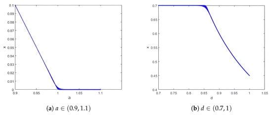
Choose the parameters $b=0.3$, $d=0.3$, $s=0.6$, with initial values $(x_0,y_0)=(1,0.1)$. We vary the prey’s effective constant-effort harvesting mortality parameter $a\in (0.9,1.1)$. From the bifurcation diagram in Figure 1a, for $a<1$, prey density persists via equilibrium $E_1$, while predator density declines to $0;$ at $a=1$, a transcritical bifurcation occurs, and prey density collapses to 0 (stable equilibrium $O(0,0)$); for $a>1$, both species go extinct (stable equilibrium $O(0,0)$). This confirms Theorem 4: $a=1$ is a critical point where the prey’s constant-effort harvesting mortality equals its intrinsic growth rate.

Figure 1. Bifurcation diagrams of system (4) at equilibrium O and $E_1,$ respectively.

Similarly, consider the parameters $b=0.3$, $a=0.3$, $s=0.6$, and the initial condition $(x_0,y_0)=(1,0.1)$. By varying the prey-to-predator conversion rate parameter $d\in (0.7,1)$, the bifurcation diagram of system (4) is shown in Figure 1b. For $d<d_0=0.857$ (where $d_0={\displaystyle \frac{s(b+1-a)}{1-a}}$), the predator density declines to 0 (stable equilibrium $E_1$). At $d=d_0$, a transcritical bifurcation occurs, and the predator density becomes positive, indicating persistence via the equilibrium $E^{*}$. For $d>d_0$, both species coexist at the stable equilibrium $E^{*}$. This validates Theorem 5: $d=d_0$ represents the minimum conversion rate required for predator persistence.

4.2. Neimark–Sacker Bifurcation

Example 2. 

Take the parameters $a=0.3$, $d=1.2$, and $s=0.6$, with initial values $(x_0,y_0)=(1,0.1)$, and vary the effective half-saturation constant b over the range $(0,0.8)$. Then, $B=p^2\left(0\right)-4q\left(0\right)=-3.4947<0$ (indicating complex eigenvalues), $\Lambda =-2.9889\ne 0$ (satisfying the transversality condition) and $\theta =-0.723<0$. Hence, a Neimark–Sacker bifurcation occurs when the effective half-saturation constant b passes through the critical value $b_0=0.3111$.

According to the phase portraits in Figure 2, for $b<b_0$ (Figure 2a–c), a repelling closed orbit surrounds the unstable equilibrium $E^{*}$, indicating population oscillations. For $b=0.3111=b_0$ (Figure 2d), $E^{*}$ is non-hyperbolic, representing a bifurcation point. For $b>b_0$ (Figure 2e,f), $E^{*}$ is stable, with no oscillations; species coexist at fixed densities. Time series for system (4) are shown in Figure 3. For $b=0.2<b_0$, the system exhibits unstable oscillations, with prey and predator densities fluctuating without convergence. For $b=0.35>b_0$, the system reaches a stable equilibrium, with densities converging to $E^{*}$. The bifurcation diagram in the $(b,x)$-plane is presented in Figure 4a, where a closed orbit emerges for $b<b_0$ and vanishes for $b>b_0$. Meanwhile, Figure 4b shows the corresponding Maximal Lyapunov Exponents for the parameter range $b\in (0,0.8)$, indicating that chaos does not occur in system (4).

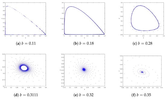
Figure 2. Phase portraits of system (4) with $a=0.3,d=1.2,s=0.6$ and different b with the initial values $(x_0,y_0)=(1,0.1)$.

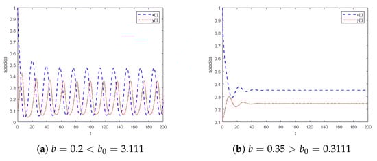
Figure 3. Time series for system (4) at $a=0.3,d=1.2,s=0.6$ and the initial value $(x_0,y_0)=(1,0.1)$.

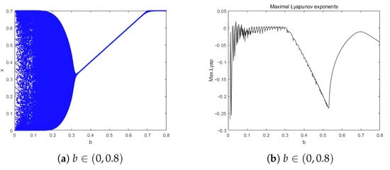
Figure 4. Bifurcation of system (4) in $(b,x)$–plane and Maximal Lyapunov Exponent.

From an ecological perspective, the paradox of enrichment persists: decreasing b (equivalent to increasing the prey carrying capacity K) destabilizes the equilibrium $E^{*}$ and induces oscillations, consistent with Rosenzweig’s original observation.

Example 3. 

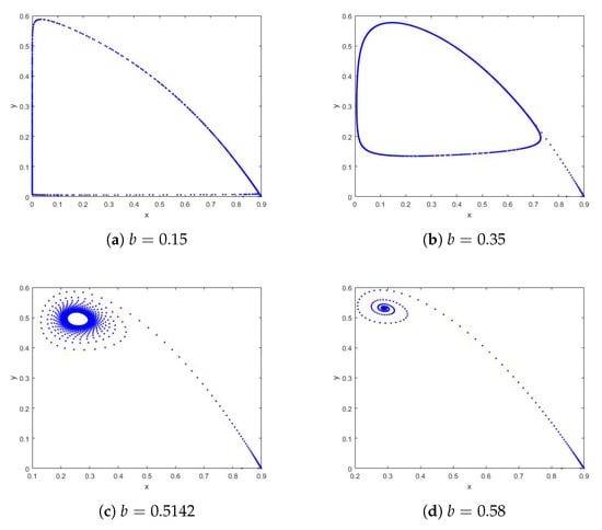
Take the parameters $a=0.1$, $d=0.3$, and $s=0.1$, with initial values $(x_0,y_0)=(0.001,0.001)$. Figure 5 shows the phase portraits of system (4) for different parameters and initial values. Figure 5a,b depict the dynamical behavior of the system, showing an unstable equilibrium $E^{*}$ with a repelling closed orbit (oscillations) for $b<b_0$. When the parameter b passes through $b_0=0.5142$, system (4) undergoes a Neimark–Sacker bifurcation, and the stability of the system at equilibrium $E^{*}$ changes accordingly. Figure 5d shows that the closed orbit shrinks and eventually disappears as the parameter b increases, resulting in a stable equilibrium $E^{*}$ (no oscillations). Similarly, the paradox of enrichment persists in system (4). This confirms that the paradox of enrichment remains intact under constant-effort harvesting, highlighting the need for cautious management of enriched ecosystems (e.g., nutrient pollution in aquatic systems).

Figure 5. Phase portraits of system (4) with $a=0.1,d=0.3,s=0.1$ and different b with the initial values $(x_0,y_0)=(0.001,0.001)$.

5. Conclusions and Management Implications

In this paper, we develop a semi-discretized Rosenzweig–MacArthur system using the piecewise constant argument method, which balances mathematical tractability with biological realism. By incorporating constant-effort harvesting on both prey and predator populations, we systematically analyze the system’s equilibrium dynamics, bifurcation behaviors, and ecological implications. Qualitative analysis reveals that the effective constant-effort harvesting induced mortality rate of prey $\left(a\right)$, the effective half-saturation constant $\left(b\right)$, the effective prey-to-predator conversion rate $\left(d\right)$, and the effective mortality rate of the predator species $\left(s\right)$ play crucial roles in determining the dynamics, especially for bifurcations, of system (4). These parameters influence both the number and stability of equilibria. We derive rigorous conditions for the existence and stability of nonnegative equilibria, including trivial, semi-trivial, and coexistence states. A transcritical bifurcation occurs at $O(0,0)$, corresponding to the prey extinction threshold $a=1$, and at $E_1(x_1,0)$, representing the predator persistence threshold $d=d_0$. Additionally, a Neimark–Sacker bifurcation arises at $E^{*}$, indicating cyclic coexistence, with the first Lyapunov coefficient quantifying the stability of the resulting closed orbit. Constant-effort harvesting parameters, defined as $a={\displaystyle \frac{q_1{e}_1}{r}}$ and $s={\displaystyle \frac{m+q_2{e}_2}{r}}$, directly affect species persistence. Maintaining $a<1$ prevents prey extinction, while setting $d>d_0$ ensures predator persistence. The paradox of enrichment persists under constant-effort harvesting—enriched ecosystems characterized by low b and high K remain susceptible to instability and oscillations. Cyclic coexistence emerges through the Neimark–Sacker bifurcation, which enables stable population cycles in the supercritical case $(\theta =-0.723<0)$, providing a plausible mechanism for observed natural dynamics such as those between lynx and hare populations.

From a biological standpoint, the key bifurcation thresholds ($a=1$, $d=d_0$, $b=b_0$) provide quantitative guidance for natural resource management and ecological regulation. The parameter $a={\displaystyle \frac{q_1{e}_1}{r}}=1$ represents the critical boundary delineating survival versus extinction for the prey population. For instance, in a crucian carp (prey)–mandarin fish (predator) system, empirical field data indicate that the intrinsic growth rate of crucian carp is $r=0.5$, corresponding to a 50% annual growth rate, while the catchability coefficient is $q_1=0.2$, standardized per fishing boat-day. When $a<1$, the critical fishing effort threshold is given by $e_1<{\displaystyle \frac{r}{q_1}}={\displaystyle \frac{0.5}{0.2}}=2.5$ boat-days per km² per year. To ensure sustainability, a seasonal fishing moratorium is implemented from March to May, coinciding with the crucian carp spawning period, and the annual fishing effort is restricted to approximately $e_1=2.0$ (e.g., 120 fishing days per year with no more than 20 boats operating daily over a 50 km² lake). Should the crucian carp population density fall below a threshold of 500 individuals per hectare, a temporary 30% reduction in fishing effort is enacted (e.g., shortening the fishing season to 80 days) to maintain a within the interval [0.6, 0.8], thereby preserving a 20–40% growth margin above the extinction threshold $a=1$.

The parameter $d=d_0$ represents the bifurcation point between decline and coexistence for predator populations. Consider a northern coastal aquaculture system involving scallop (prey)–swimming crab (predator) interactions. Scallops are the primary cultured species, while swimming crabs naturally regulate scallop overpopulation. The goal is to sustain swimming crab populations by ensuring $d>d_0$, where $d_0={\displaystyle \frac{s(b+1-a)}{1-a}}$ is the minimum prey-to-predator conversion rate required for predator persistence. For swimming crabs, the overall mortality rate is $s=0.3$ (reflecting 30% annual mortality, including natural causes and incidental fishing), the half-saturation constant is $b=0.4$, and the scallop harvesting-induced mortality rate is $a=0.2$, representing moderate harvesting that balances yield with the crabs’ food supply. The critical conversion rate is thus calculated as $d_0={\displaystyle \frac{0.3\times (0.4+1-0.2)}{1-0.2}}\approx 0.38$. To increase prey density and raise d to values between 0.4 and 0.5, exceeding $d_0$, 5000 scallop seeds per hectare are stocked annually in spring. Additionally, deploying artificial reefs at a density of one reef per 10 hectares provides shelter for crabs, thereby reducing natural mortality s and indirectly lowering the critical threshold $d_0$.

The parameter $b=b_0$ governs the transition between stability and oscillation within the system dynamics. This is exemplified by a phytoplankton (prey)–cladoceran (predator) system. Elevated nutrient inputs, notably nitrogen and phosphorus, increase the phytoplankton carrying capacity K, which in turn reduces the half-saturation constant $b={\displaystyle \frac{h}{K}}$, where h denotes the Holling Type II half-saturation constant. Such a reduction precipitates population oscillations ($b<b_0$) as a manifestation of the paradox of enrichment. Management strategies thus aim to stabilize coexistence by maintaining $b>b_0$, where the critical value is defined as $b_0={\displaystyle \frac{(1-a)(d-s)(1+d-s)}{d+s(1+d-s)}}$. For cladocerans, the conversion rate is $d=1.2$, the comprehensive mortality rate is $s=0.6$, and the phytoplankton harvesting-induced mortality rate is $a=0.3$, the latter resulting from filter-feeding fish activity. Under these conditions, the critical half-saturation constant is approximately $b_0\approx 0.31$. Ecological floating beds covering 20% of the lake surface area should be installed at the inflow points to facilitate the absorption of nitrogen and phosphorus, thereby decreasing the phytoplankton carrying capacity K. This intervention is expected to increase the parameter b from 0.25, indicative of a eutrophic state, to a range of $0.35–0.4$, surpassing the threshold value $b_0=0.31$. Additionally, the introduction of filter-feeding silver carp at a stocking density of 50 individuals per hectare is recommended to regulate phytoplankton density and prevent the parameter b from declining.

In future research, the model will focus on two key extensions and will be expanded to incorporate time-varying harvesting, including seasonal harvesting, represented by $a\left(t\right)$ for prey harvesting effort and $s\left(t\right)$ for predator harvesting-induced mortality. This extension is anticipated to yield more complex dynamical behaviors, such as quasi-periodicity, compared to models with constant-effort harvesting. Additionally, diffusion processes will be integrated into the discrete system to examine spatial pattern formation associated with spatial Turing instability and temporal Neimark–Sacker bifurcation, potentially resulting in spatiotemporal chaos characterized by chaotic dynamics across both spatial and temporal dimensions.

References

- Rosenzweig, M.L.; MacArthur, R.H. Graphical representation and stability conditions of predator-prey interactions. Am. Nat. 1963, 97, 209–223. [Google Scholar] [CrossRef]
- Upadhyay, R.K.; Roy, P.; Datta, J. Complex dynamics of ecological systems under nonlinear harvesting: Hopf bifurcation and Turing instability. Nonlinear Dyn. 2015, 79, 2251–2270. [Google Scholar] [CrossRef]
- May, R.M.; Beddington, J.R.; Clark, C.W.; Holt, S.J.; Laws, R.M. Management of multispecies fisheries. Science 1979, 205, 267–277. [Google Scholar] [CrossRef] [PubMed]
- Misra, O.P.; Babu, A.R. Modelling the effect of toxicant on a three species food-chain system with predator harvesting. Int. J. Appl. Comput. Math. 2017, 3, 71–97. [Google Scholar] [CrossRef]
- Liu, K.; Yang, W. Ecological dynamics of a delayed predator–prey model with prey refuge and nonlinear harvesting. Comput. Appl. Math. 2025, 44, 404. [Google Scholar] [CrossRef]
- Roy, D.; Ghosh, B. Dimensionally homogeneous fractional order Rosenzweig–MacArthur model: A new perspective of paradox of enrichment and harvesting. Nonlinear Dyn. 2024, 112, 18137–18161. [Google Scholar] [CrossRef]
- Shang, Z.C.; Qiao, Y.H.; Juan, L.J.; Miao, J. Bifurcation analysis in a predator–prey system with an increasing functional response and constant-yield prey harvesting. Math. Comput. Simul. 2021, 190, 976–1002. [Google Scholar] [CrossRef]
- Xiang, C.; Lu, M.; Huang, J.C. Degenerate Bogdanov-Takens bifurcation of codimension 4 in Holling-Tanner model with harvesting. J. Differ. Equ. 2022, 314, 370–417. [Google Scholar] [CrossRef]
- Bandyopadhyay, R.; Chattopadhyay, J. The impact of harvesting on the evolutionary dynamics of prey species in a prey-predator systems. J. Math. Biol. 2024, 89, 38. [Google Scholar] [CrossRef]
- Huang, J.; Gong, Y.; Ruan, S. Bifurcation analysis in a predator–prey model with constant-yield predator harvesting. Discret. Contin. Dyn. Syst. Ser. B 2013, 18, 2101–2121. [Google Scholar] [CrossRef]
- Huang, J.; Gong, Y.; Chen, J. Multiple bifurcations in a predator–prey system of Holling and Leslie type with constant-yield prey harvesting. Int. J. Bifurc. Chaos 2013, 23, 1350164. [Google Scholar] [CrossRef]
- Ahmidi, M.; Mokni, K.; Ch-Chaoui, M. Influence of Prey Harvesting on the Dynamics of a Prey–Predator System: Multi-Parameter Bifurcation Analysis. Nonlinear Dyn. 2025, 113, 31841–31870. [Google Scholar] [CrossRef]
- Biswas, S.; Bhutia, L.T.; Kar, T.K. Impact of the herd harvesting on a temporal and spatiotemporal prey–predator model with certain prey herd behaviors and density-dependent cross-diffusion. Eur. Phys. J. Plus 2024, 139, 1101. [Google Scholar] [CrossRef]
- Mortuja, M.; Chaube, M.; Kumar, S. Dynamic analysis of a predator-prey model with Michaelis-Menten prey harvesting and hunting cooperation in predators. J. Appl. Math. Comput. 2025, 71, 6207–6229. [Google Scholar] [CrossRef]
- Lv, Y.F.; Pei, Y.Z.; Gao, S.J.; Li, C.G. Harvesting of a phytoplankton–zooplankton model. Nonlinear Anal. Real World Appl. 2010, 11, 3608–3619. [Google Scholar] [CrossRef]
- Makinde, O.D. Solving ratio-dependent predator–prey system with constant effort harvesting using Adomian decomposition method. Appl. Math. Comput. 2007, 186, 17–22. [Google Scholar] [CrossRef]
- Rainj, B.G. Multistability, chaos and mean population density in a discrete-time predator–prey system. Chaos Solitons Fractals 2022, 162, 112497. [Google Scholar]
- Jiao, J.; Xiao, Y.; Jiao, H. Dynamics of a switched predator–prey breeding management model with impulsive nonlinear releasing and age-selective harvesting predator. Adv. Contin. Discret. Model. 2025, 2025, 101. [Google Scholar] [CrossRef]
- Mortuja, M.G.; Chaube, M.K.; Kumar, S. Dynamic analysis of a predator-prey system with nonlinear prey harvesting and square root functional response. Chaos Solitons Fractals 2018, 148, 111071. [Google Scholar] [CrossRef]
- Tiwari, V.; Thipathi, J.P.; Abbas, S.; Wang, J.S.; Sun, G.Q.; Jin, Z. Qualitative analysis of a diffusive Crowley–Martin predator–prey model: The role of nonlinear predator harvesting. Nonlinear Dyn. 2019, 98, 1169–1189. [Google Scholar] [CrossRef]
- Singh, A.; Sharma, V.S. Bifurcations and chaos control in a discrete-time prey–predator model with Holling type-II functional response and prey refuge. J. Comput. Appl. Math. 2023, 418, 114666. [Google Scholar] [CrossRef]
- Lei, C.; Han, X.L.; Wang, W.M. Bifurcation analysis and chaos control of a discrete-time prey-predator model with fear factor. Math. Biosci. Eng. 2022, 19, 6659–6679. [Google Scholar] [CrossRef] [PubMed]
- Din, Q. Complexity and chaos control in a discrete-time prey-predator model. Commun. Nonlinear Sci. Numer. Simul. 2017, 49, 113–134. [Google Scholar] [CrossRef]
- Dhar, J.; Singh, H.; Bhatti, H.S. Discrete-time dynamics of a system with crowding effect and predator partially dependent on prey. Appl. Math. Comput. 2015, 252, 324–335. [Google Scholar] [CrossRef]
- Hu, D.; Cao, H.J. Bifurcation and chaos in a discrete-time predator–prey system of Holling and Leslie type. Commun. Nonlinear Sci. Numer. Simul. 2015, 22, 702–715. [Google Scholar] [CrossRef]
- Ruan, M.; Li, C.; Li, X. Codimension two 1:1 strong resonance bifurcation in a discrete predator-prey model with Holling IV functional response. AIMS Math. 2022, 7, 3150–3168. [Google Scholar] [CrossRef]
- Yao, W.; Li, X. Bifurcation difference induced by different discrete methods in a discrete predator-prey model. J. Nonlinear Model. Anal. 2022, 4, 64–79. [Google Scholar]
- Winggins, S. Introduction to Applied Nonlinear Dynamical Systems and Chaos; Springer: New York, NY, USA, 2003. [Google Scholar]
- Murray, J.D. Mathematical Biology, 2nd ed.; Springer: Berlin, Germany, 1993. [Google Scholar]
- Kuzenetsov, Y.A. Elements of Applied Bifurcation Theory, 2nd ed.; Springer: New York, NY, USA, 1998. [Google Scholar]
- Min, N.; Xing, P.; Zhang, H. Role of Allee effect, hunting cooperation, and prey harvesting in a Leslie–Gower predator–prey model. Adv. Contin. Discret. Model. 2025, 2025, 96. [Google Scholar] [CrossRef]
- Ruan, M.; Li, X. Complex dynamical properties and chaos control for a discrete modified Leslie-Gower prey-predator system with Holling II functional response. Adv. Contin. Discret. Model. 2024, 2024, 30. [Google Scholar] [CrossRef]
Disclaimer/Publisher’s Note: The statements, opinions and data contained in all publications are solely those of the individual author(s) and contributor(s) and not of MDPI and/or the editor(s). MDPI and/or the editor(s) disclaim responsibility for any injury to people or property resulting from any ideas, methods, instructions or products referred to in the content. |
© 2025 by the authors. Licensee MDPI, Basel, Switzerland. This article is an open access article distributed under the terms and conditions of the Creative Commons Attribution (CC BY) license (https://creativecommons.org/licenses/by/4.0/).