Analysis of Oscillatory Behavior of Second-Order Neutral Delay Difference Equations

Abstract

The paper investigates the oscillation, zero-convergence, and solutions of second-order neutral delay difference equations containing three nonlinear delayed terms with different growth rates. By using positivity and monotonicity conditions on an auxiliary function along with divergence-type conditions on the coefficient sequences of the neutral and delayed terms, the paper establishes new criteria that guarantee oscillation or convergence of all solutions. These novel findings extend and enhance several of the existing oscillation criteria established by the literature. Suggestions for further investigation are included with illustrative examples.

1. Introduction

Difference equations constitute a fundamental tool for modelling discrete dynamical systems and serve as the natural discrete analogue of differential equations. They find widespread applications in population biology, economics, numerical analysis, control theory, and many other fields. The inclusion of delay arguments allows these equations to capture memory effects and historical dependence, making delay difference equations particularly suitable for systems where past states significantly influence the current evolution [1,2,3]. Neutral delay difference equations, in which the delay appears inside the principal difference operator, exhibit even richer dynamics and have therefore attracted considerable attention in recent years [4,5].

The present paper is devoted to the oscillatory behavior of all solutions of the second-order linear neutral delay difference equation

$$\Delta \left(m_l{\left(\Delta ({\mathrm{Y}}_l+n_l\mathrm{Y}({\eta }_l))\right)}^{\sigma }\right)+p_l{\mathrm{Y}}^{\beta }({\gamma }_l)+q_l{\mathrm{Y}}^{\mu }({\tau }_l)=0,$$

(1)

where $\sigma$, $\beta$, and $\mu$ are ratios of odd positive integers, the sequences $m_l$, $p_l$, $q_l$, and $n_l$ are positive real numbers with $|n_l|<\infty$, and the delay (and advanced) arguments satisfy ${\eta }_l\le l$, ${\gamma }_l\le l$, ${\tau }_l\le l$ with ${\lim }_{l\to \infty }{\eta }_l={\lim }_{l\to \infty }{\gamma }_l={\lim }_{l\to \infty }{\tau }_l=\infty$. Our main objective is to derive new sufficient conditions ensuring that every solution of (1) oscillates, without resorting to comparison principles. The results are established under either of the structural assumptions $(G_1){\sum }_{l=0}^{\infty }{\displaystyle \frac{1}{m_l}}=\infty \mathrm{or}(G_2){\sum }_{l=0}^{\infty }{\displaystyle \frac{1}{m_l}}<\infty$ and hold for all admissible bounded neutral coefficients $n_l$.

Difference equations play a fundamental role in the analysis of discrete dynamical systems, providing a natural framework for modeling processes that evolve at distinct time steps. They serve as the discrete counterpart of differential equations and appear in diverse applications, including population biology, economics, numerical simulations, and control theory. When delays are incorporated, difference equations capture memory effects by linking the present state of the system to its past values [1,2,3]. In particular, neutral difference equations, where delayed terms occur inside the principal difference operator, exhibit richer and more intricate dynamics. Understanding the oscillatory behavior of their solutions is essential for characterizing stability, cyclic patterns, and long-term system behavior. This motivates the development of new criteria that ensure oscillation or convergence of solutions under general structural and coefficient conditions [4,5].

Delay difference equations (DDEs) are unique in that they account for the system’s past states. By including these historical effects, DDEs allow for more accurate and effective predictions about the future behavior of the system, especially in cases where past events play a critical role in current dynamics [6,7,8]. The study of oscillation in neutral difference equations has attracted considerable attention due to their ability to model dynamic processes in which the future state depends not only on delayed values but also on delayed differences of the unknown function. Unlike ordinary or simple delay difference equations, neutral difference equations include terms where the delay appears inside the main difference operator, making their qualitative behavior more complex [9,10,11]. In recent years, researchers have focused on developing oscillation criteria for neutral difference equations under various structural assumptions. Many existing results treat cases with a single nonlinear delayed term or assume that all exponents appearing in the nonlinear terms are equal. However, real-world systems often involve several delayed components with different growth rates. This motivates the study of neutral difference equations with multiple nonlinear terms and distinct exponents, requiring more refined analytical tools and conditions to determine whether solutions oscillate or tend to zero [12,13]. The present work contributes to this direction by establishing new oscillation criteria for second-order neutral difference equations under general exponent settings and coefficient conditions. These results unify and extend previous findings for special cases of neutral difference equations and provide a broader framework applicable to systems with more complex nonlinear interactions [14,15,16].

In the qualitative theory of difference equations, oscillatory behavior is of central importance [17,18]. A nontrivial solution is said to be oscillatory if it is neither eventually positive nor eventually negative. This behavior arises naturally in numerous physical systems, including vibrating mechanical systems, electrical circuits, and interacting particle systems governed by electromagnetic forces with finite propagation speed [3,4,5,9,10,19,20,21]. When propagation delays are taken into account, and the governing physical laws are symmetric under time reversal, both delayed (retarded) and advanced terms appear in equations [11,16,22,23,24,25]. This delayed–advanced interaction has been recognized since the early work of Tetrode, Fokker, Wheeler, Feynman, and later Driver and Hoag. For general background on difference equations, refer to the monographs [6,7,12,13] and the numerous recent contributions on oscillation and non-oscillation of neutral delay difference equations, among which we particularly mention [9,10,11,22,23,24] and the references therein.

2. Main Result

Sufficient Conditions for Oscillation Criteria

Throughout the discussion, this notation is used

$$x_l={\mathrm{Y}}_l+n_l\mathrm{Y}({\eta }_l).$$

(2)

Lemma 1

([26]). Let $n_l\ge 0$. Suppose that $(G_1)$ holds. If ${\mathrm{Y}}_l$ is an eventually positive solution of (1), then the corresponding function $x_l={\mathrm{Y}}_l+n_l\mathrm{Y}({\eta }_l)$ satisfies $x_l>0$, $\Delta (x_l)>0$, $\Delta (m_l{(\Delta x_l)}^{\sigma })\le 0,$ for any large value of l, where σ is a quotient of odd positive integers.

Lemma 2

([26]). Assume that

$$P\ge 0,Q\ge 0and\theta \ge 1.Thenweget$$

$${(P+Q)}^{\theta }\le 2^{\theta -1}(P^{\theta }+Q^{\theta }).$$

(3)

If $0<\theta \le 1,$ then

$${(P+Q)}^{\theta }\le (P^{\theta }+Q^{\theta }).$$

Now, suppose that $0\le n_l\le g<\infty$, $\eta ({\gamma }_l)=\gamma ({\eta }_l)$ and $\eta ({\tau }_l)=\tau ({\eta }_l)$ for all $l>0$.

Theorem 1.

Let $\sigma =\beta =\mu$ and $(G_1)$ hold. Suppose that

$$\sum _{l=l_0}^{\infty }{2}^{1-\beta }{R}^{\mu }\left[B_l+A_l\right]=\infty ,$$

(4)

where

$$B_l=min\{p_l,p({\eta }_l)\},A_l=min\{q_l,q({\eta }_l)\}.$$

Then every solution of (1) oscillates.

Proof. 

By contradiction, assume that ${\mathrm{Y}}_l$ is a non-oscillatory solution of (1). Without loss of generality, we can assume that ${\mathrm{Y}}_l>0$ for $l\ge l_0$. Consequently there exists $l_1\ge l_0$ such that ${\mathrm{Y}}_l>0$, $\mathrm{Y}({\eta }_l)>0$, $\mathrm{Y}({\gamma }_l)>0$, and $\mathrm{Y}({\tau }_l)>0$ for $l\ge l_1$. By (1), it becomes

$$\Delta (m_l{(\Delta x_l)}^{\sigma })=-p_l{\mathrm{Y}}^{\beta }({\gamma }_l)-q_l{\mathrm{Y}}^{\mu }({\tau }_l)\le 0,notidenticallyzeroforl\ge l_1.$$

(5)

Thus, $m_l{(\Delta x_l)}^{\sigma }$ is non-increasing that is, either $\Delta x_l>0$ or $\Delta x_l<0$. According to Lemma 1, it results that $\Delta x_l>0$ for $l\ge l_2$. From (1), it is easy to see that

$$\begin{array}{cc}\hfill \Delta (m_l{(\Delta x_l)}^{\sigma })& +g^{\beta }\Delta (m({\eta }_l))(\Delta x{({\eta }_l)}^{\sigma })+p_l{\mathrm{Y}}^{\beta }({\gamma }_l)+g^{\beta }p({\eta }_l){\mathrm{Y}}^{\beta }(\gamma ({\eta }_l))+q_l{\mathrm{Y}}^{\mu }({\tau }_l)\hfill \\ & +g^{\beta }q({\eta }_l){\mathrm{Y}}^{\mu }(\tau ({\eta }_l))=0forl\ge l_1.(since\sigma =\beta =\mu ).\hfill \end{array}$$

(6)

By Lemma 2, (6) implies that

$$\Delta (m_l{(\Delta x_l)}^{\sigma })+g^{\beta }\Delta (m({\eta }_l))(\Delta x{({\eta }_l)}^{\sigma })+2^{1-\beta }{B}_l{x}^{\mu }({\gamma }_l)+2^{1-\beta }{A}_l{x}^{\mu }({\tau }_l)\le 0.$$

(7)

By Lemma 2, it follows that $x_l$ is non-decreasing and hence $x_l\ge R$ for $l\ge l_2>l_1$.

• Hence, (7) implies that

$$\Delta (m_l{(\Delta x_l)}^{\sigma })+g^{\beta }\Delta (m({\eta }_l))(\Delta x{({\eta }_l)}^{\sigma })+2^{1-\beta }{B}_l{R}^{\mu }+2^{1-\beta }{A}_l{R}^{\mu }\le 0.$$

Then there exists $l_3>l_2$ such that

$$2^{1-\beta }{B}_l{R}^{\mu }+2^{1-\beta }{A}_l{R}^{\mu }\le -\Delta (m_l{(\Delta x_l)}^{\sigma })-g^{\beta }\Delta (m({\eta }_l)(\Delta x{({\eta }_l)}^{\sigma })),$$

(8)

for $l\ge l_3$.

• Summing (8) from $l_{3}to\infty$, we obtain a contradiction to (4). This concludes the proof of the theorem. □

Theorem 2.

Let $\sigma >\beta >\mu$. If $(G_1)$ and (4) hold, then every solution of (1) oscillates.

Proof. 

By contradiction, assume that ${\mathrm{Y}}_l$ is a non-oscillatory solution of (1). Without loss of generality, we may assume that ${\mathrm{Y}}_l>0$ for $l\ge l_0$. So there exists $l_1>l_0$ such that ${\mathrm{Y}}_l>0$, $\mathrm{Y}({\eta }_l)>0$, $\mathrm{Y}({\gamma }_l)>0$ and $\mathrm{Y}({\tau }_l)>0$ for $l\ge l_1$. By using (1), it becomes

$$\Delta (m_l{(\Delta x_l)}^{\sigma })=-p_l{\mathrm{Y}}^{\beta }({\gamma }_l)-q_l{\mathrm{Y}}^{\mu }({\tau }_l)\le 0,\mathrm{not}\mathrm{identically}\mathrm{zero}\mathrm{for}\mathrm{l}\ge {\mathrm{l}}_1.$$

Thus $m_l{(\Delta x_l)}^{\sigma }$ is non-increasing that is, either $\Delta x_l>0$ or $\Delta x_l<0$. According to Lemma 1, it follows that $\Delta x_l>0$ for $l\ge l_2$. From (1), it is easy to see that

$$\begin{array}{cc}\hfill \Delta (m_l{(\Delta x_l)}^{\sigma })& +g^{\beta }\Delta (m({\eta }_l))(\Delta x{({\eta }_l)}^{\sigma })+p_l{\mathrm{Y}}^{\beta }({\gamma }_l)+g^{\beta }p({\eta }_l){\mathrm{Y}}^{\beta }(\gamma ({\eta }_l))+q_l{\mathrm{Y}}^{\mu }({\tau }_l)\hfill \\ & +g^{\beta }q({\eta }_l){\mathrm{Y}}^{\mu }(\tau ({\eta }_l))=0forl\ge l_1.(since\sigma >\beta >\mu ).\hfill \end{array}$$

(9)

By Lemma 2, (9) implies that

$$\Delta (m_l{(\Delta x_l)}^{\sigma })+g^{\beta }\Delta (m({\eta }_l))(\Delta x{({\eta }_l)}^{\sigma })+2^{1-\beta }{B}_l{x}^{\mu }({\gamma }_l)+2^{1-\beta }{A}_l{x}^{\mu }({\tau }_l)\le 0.$$

(10)

By Lemma 2, it follows that $x_l$ is non-decreasing and hence $x_l\ge R$ for $l\ge l_2>l_1$. Hence (10) implies that

$$\Delta (m_l{(\Delta x_l)}^{\sigma })+g^{\beta }\Delta (m({\eta }_l))(\Delta x{({\eta }_l)}^{\sigma })+2^{1-\beta }{B}_l{R}^{\mu }+2^{1-\beta }{A}_l{R}^{\mu }\le 0.$$

Hence there exists $l_3>l_2$ such that

$$2^{1-\beta }{B}_l{R}^{\mu }+2^{1-\beta }{A}_l{R}^{\mu }\le -\Delta (m_l{(\Delta x_l)}^{\sigma })-g^{\beta }\Delta (m({\eta }_l)(\Delta x{({\eta }_l)}^{\sigma })),$$

(11)

for $l\ge l_3$. Summing (11) from $l_{3}to\infty$, we obtain a contradiction to (4). This concludes the proof of the theorem. □

Theorem 3.

Let $\sigma <\beta <\mu$. Suppose that $(G_1)$ holds and

$$\sum _{l=l_0}^{\infty }{2}^{1-\mu }{R}^{\beta }\left[B_l+A_l\right]=\infty$$

(12)

holds. Then every solution of (1) oscillates.

Proof. 

By contradiction, assume that ${\mathrm{Y}}_l$ is a non-oscillatory solution of (1). Without loss of generality, we may assume that ${\mathrm{Y}}_l>0$ for $l\ge l_0$. So there exits $l_1>l_0$ such that ${\mathrm{Y}}_l>0$, $\mathrm{Y}({\eta }_l)>0$, $\mathrm{Y}({\gamma }_l)>0$ and $\mathrm{Y}({\tau }_l)>0$ for $l\ge l_1$.

• By using (1), it becomes

$$\Delta (m_l{(\Delta x_l)}^{\sigma })=-p_l{\mathrm{Y}}^{\beta }({\gamma }_l)-q_l{\mathrm{Y}}^{\mu }({\tau }_l)\le 0,\mathrm{not}\mathrm{identically}\mathrm{zero}\mathrm{for}\mathrm{l}\ge {\mathrm{l}}_1.$$

Thus $m_l{(\Delta x_l)}^{\sigma }$ is non-increasing that is, either $\Delta x_l>0$ or $\Delta x_l<0$. According to Lemma 1, it follows that $\Delta x_l>0$ for $l\ge l_2$. From (1), it is easy to see that

$$\begin{array}{cc}\hfill \Delta (m_l{(\Delta x_l)}^{\sigma })& +g^{\mu }\Delta (m({\eta }_l))(\Delta x{({\eta }_l)}^{\beta })+p_l{\mathrm{Y}}^{\beta }({\gamma }_l)+g^{\beta }p({\eta }_l){\mathrm{Y}}^{\beta }(\gamma ({\eta }_l))+q_l{\mathrm{Y}}^{\mu }({\tau }_l)\hfill \\ & +g^{\beta }q({\eta }_l){\mathrm{Y}}^{\mu }(\tau ({\eta }_l))=0forl\ge l_1.(since\sigma >\beta >\mu ).\hfill \end{array}$$

(13)

By Lemma 2, (13) implies that

$$\Delta (m_l{(\Delta x_l)}^{\sigma })+g^{\beta }\Delta (m({\eta }_l))(\Delta x{({\eta }_l)}^{\sigma })+2^{1-\beta }{B}_l{x}^{\mu }({\gamma }_l)+2^{1-\beta }{A}_l{x}^{\mu }({\tau }_l)\le 0.$$

(14)

By Lemma 2, it follows that $x_l$ is non-decreasing and hence $x_l\ge R$ for $l\ge l_2>l_1$. Hence, (10) implies that

$$\Delta (m_l{(\Delta x_l)}^{\sigma })+g^{\beta }\Delta (m({\eta }_l))(\Delta x{({\eta }_l)}^{\sigma })+2^{1-\beta }{B}_l{R}^{\mu }+2^{1-\beta }{A}_l{R}^{\mu }\le 0.$$

Hence, there exists $l_3>l_2$ such that

$$2^{1-\beta }{B}_l{R}^{\mu }+2^{1-\beta }{A}_l{R}^{\mu }\le -\Delta (m_l{(\Delta x_l)}^{\sigma })-g^{\beta }\Delta (m({\eta }_l)(\Delta x{({\eta }_l)}^{\sigma })),$$

(15)

for $l\ge l_3$. Summing (15) from $l_{3}to\infty$, we obtain a contradiction to (4). This concludes the proof of the theorem. □

Moreover, assume that $-1<g\le n_l\le 0$.

Theorem 4.

Let $\sigma >\beta >\mu$. Assume that $(G_1)$ holds.

$$\sum _{s=l_0}^{\infty }\left[p_s+q_s\right]=\infty$$

(16)

and

$$\sum _{s=l_0}^{\infty }\left[p({\eta }_s)+q({\eta }_s)\right]=\infty .$$

(17)

Then every solution of (1) oscillates or tends to zero as $l\to \infty$.

Proof. 

By contradiction, assume that ${\mathrm{Y}}_l$ is a non-oscillatory solution of (1). Without loss of generality, we can assume that ${\mathrm{Y}}_l>0$ for $l\ge l_0$. Consequently there exists $l_1\ge l_0$ such that ${\mathrm{Y}}_l>0$, $\mathrm{Y}({\eta }_l)>0$, $\mathrm{Y}({\gamma }_l)>0$ and $\mathrm{Y}({\tau }_l)>0$ for $l\ge l_1$. By (1), it becomes

$$\Delta (m_l{(\Delta x_l)}^{\sigma })=-p_l{\mathrm{Y}}^{\beta }({\gamma }_l)-q_l{\mathrm{Y}}^{\mu }({\tau }_l)\le 0,notidenticallyzeroforl\ge l_1.$$

(18)

Suppose that $x_l$ and $\Delta x_l$ are monotonic functions. If $\Delta x_l<0$ for $l\ge l_2$, then $\Delta (m_l{(\Delta x_l)}^{\sigma })\le 0$ implies that

$$m_l{(\Delta x_l)}^{\sigma }\le m_{l_2}{(\Delta x_{l_2})}^{\sigma },$$

That is,

$${(\Delta x_l)}^{\sigma }\le {\displaystyle \frac{m_{l_2}{(\Delta x_{l_2})}^{\sigma }}{m_l}},$$

(19)

Summing (18) from $l_{1}tol-1$,

$$x_l\le x_{l_1}+m_{l_2}^{{\displaystyle \frac{1}{\sigma }}}\Delta (x_{l_2})\sum _{s=l_1}^{l-1}{\displaystyle \frac{1}{m_s^{\frac{1}{\sigma }}}}\to -\infty asl\to \infty ,$$

which is absurd given the fact that $x_l>0$. Moreover, the contradiction mentioned above is true if $x_l<0.$ Indeed ${\mathrm{Y}}_l$ is bounded when $x_l<0$. Assume that this does not hold. Then there exists a sequence of points $\left\{t_r\right\}$ such that $t_r\to \infty$ as $r\to \infty$ and $\mathrm{Y}(t_r)=max\{{\mathrm{Y}}_l:l_3\le l\le t_r\}$. Given that $\gamma (t_r)\le t_r,$$\mathrm{Y}(\gamma (t_r))\le \mathrm{Y}(t_r)$ implies that

$$\begin{array}{cc}\hfill x(t_r)& \ge \mathrm{Y}(t_r)+g\mathrm{Y}(\gamma (t_r))\hfill \\ \hfill & =(1+g)\mathrm{Y}(t_r)(since1+g>0)\hfill \\ \hfill & \to +\infty asr\to \infty ,\hfill \end{array}$$

which is a contradiction. Consequently, ${\mathrm{Y}}_l$ is bounded and $\underset{l\to \infty }{\lim }{x}_l$ exists. As a consequence, we address the following two cases,

$$(i)x_l>0,\Delta x_l>0,(ii)x_l<0,\Delta x_l>0.$$

Case (i): In this case, $x_l\le {\mathrm{Y}}_l$ and $\underset{l\to \infty }{\lim }{m}_l\Delta x_l$ exists. Thus, (1) becomes

$$\Delta (m_l{(\Delta x_l)}^{\sigma })+p_l{\mathrm{Y}}^{\beta }({\gamma }_l)+q_l{\mathrm{Y}}^{\mu }({\tau }_l)\le 0$$

(20)

for $l\ge l_3>l_2$, since $\sigma >\beta >\mu$. Using Lemma 2, we obtain $x_l\ge R.$ Therefore (19) gives that

$$\Delta (m_l{(\Delta x_l)}^{\sigma })+p_l{R}^{\mu }+q_l{R}^{\mu }\le 0,$$

$$R^{\mu }\left[p_l+q_l\right]\le -\Delta (m_l{(\Delta x_l)}^{\sigma }).$$

(21)

Summing (20) from $l_{3}to+\infty$, we have a contradiction to (16).

• Case (ii): Let $\underset{l\to \infty }{\lim }{x}_l$ and $\underset{l\to \infty }{\lim }{x}_l=\rho$ exist we say that $\rho =0$. If not, then there exists $t<0$ and $l_3>l_2$ such that

$$x({\gamma }_l)\le x_l<t,x({\tau }_l)\le x_l<tforl\ge l_3.$$

By (1), it follows that $x_l>g\mathrm{Y}({\eta }_l)$ and hence $\mathrm{Y}(\eta ({\gamma }_l))>{\displaystyle \frac{1}{g}}x({\gamma }_l)$;

• that is,

$$\mathrm{Y}(\gamma ({\eta }_l))>({\displaystyle \frac{t}{g}})forl\ge l_3.$$

Additionally, $\mathrm{Y}(\tau ({\eta }_l))>\left({\displaystyle \frac{t}{g}}\right)$ for $l\ge l_3.$ According to (1), it can be written as

$$\Delta (m({\eta }_l))(\Delta x{({\eta }_l)}^{\sigma })+p({\eta }_l){\mathrm{Y}}^{\beta }(\gamma ({\eta }_l))+q({\eta }_l){\mathrm{Y}}^{\mu }(\tau ({\eta }_l))=0$$

for $l\ge l_3,$ we obtain

$$\Delta (m({\eta }_l))(\Delta x{({\eta }_l)}^{\sigma })+{\left({\displaystyle \frac{t}{g}}\right)}^{\mu }p({\eta }_l)+{\left({\displaystyle \frac{t}{g}}\right)}^{\mu }q({\eta }_l)\le 0.(since\sigma >\beta >\mu ).$$

(22)

Summing (22) from $l_{3}tol-1$, we get

$$\begin{array}{ll}{\left({\displaystyle \frac{t}{g}}\right)}^{\mu }\left[{\displaystyle \sum _{s=l_3}^{l-1}}p({\eta }_s)+{\displaystyle \sum _{s=l_3}^{l-1}}q({\eta }_s)\right]& \le -[\Delta (m({\eta }_l)(\Delta x{({\eta }_l)}^{\sigma }))-\Delta (m(\eta (l_3))(\Delta x{(\eta (l_3))}^{\sigma }))]\\ & <-\Delta (m({\eta }_l)(\Delta x{({\eta }_l)}^{\sigma }))<\infty asl\to \infty ,\end{array}$$

which is a contradiction to (17). Hence $\rho =0.$ Applying the same reason as before, it is easy to show that ${\mathrm{Y}}_l$ is bounded. Therefore,

$$\begin{array}{cc}\hfill 0\ge \underset{l\to \infty }{\lim }{x}_l& =\underset{l\to \infty }{\lim }sup{x}_l\hfill \\ \hfill & \ge \underset{l\to \infty }{\lim }sup(({\mathrm{Y}}_l)+g\mathrm{Y}({\eta }_l))\hfill \\ \hfill & \ge \underset{l\to \infty }{\lim }sup({\mathrm{Y}}_l)+\underset{l\to \infty }{\lim }inf(g\mathrm{Y}({\eta }_l))\hfill \\ \hfill & =\underset{l\to \infty }{\lim }sup{\mathrm{Y}}_l+g\underset{l\to \infty }{\lim }sup(\mathrm{Y}({\eta }_l))\hfill \\ \hfill & =(1+g)\underset{l\to \infty }{\lim }sup{\mathrm{Y}}_l,\hfill \end{array}$$

which implies that $\underset{l\to \infty }{\lim }sup{\mathrm{Y}}_l=0$; that is, $\underset{l\to \infty }{\lim }{\mathrm{Y}}_l=0.$ This completes the proof of the theorem. □

Theorem 5.

Let $\sigma <\beta <\mu .$ If $(G_1)$, (16) and (17) hold, then every solution of (1) oscillates or tends to zero as $l\to \infty .$

Proof. 

By contradiction, assume that ${\mathrm{Y}}_l$ is a non-oscillatory solution of (1). Without loss of generality, we can assume that ${\mathrm{Y}}_l>0$ for $l\ge l_0$. Consequently there is $l_1\ge l_0$ such that ${\mathrm{Y}}_l>0$, $\mathrm{Y}({\eta }_l)>0$, $\mathrm{Y}({\gamma }_l)>0$ and $\mathrm{Y}({\tau }_l)>0$ for $l\ge l_1$. By (1), it becomes

$$\Delta (m_l{(\Delta x_l)}^{\sigma })=-p_l{\mathrm{Y}}^{\beta }({\gamma }_l)-q_l{\mathrm{Y}}^{\mu }({\tau }_l)\le 0,notidenticallyzeroforl\ge l_1.$$

(23)

Suppose that $x_l$ and $\Delta x_l$ are monotonic functions. We consider the following four possible cases:

$$(i)x_l>0,\Delta x_l>0,(ii)x_l<0,\Delta x_l>0,$$

$$(iii)x_l>0,\Delta x_l<0,(iv)x_l<0,\Delta x_l<0.$$

Case (i): In this case, $x_l\le {\mathrm{Y}}_l$ and $\underset{l\to \infty }{\lim }{m}_l\Delta x_l$ exists. Thus, (1) becomes

$$\Delta (m_l{(\Delta x_l)}^{\sigma })+p_l{x}^{\beta }({\gamma }_l)+q_l{x}^{\mu }({\tau }_l)\le 0.(since\sigma <\beta <\mu )$$

(24)

for $l\ge l_3>l_2$. Using Lemma 2, we obtain $x_l\ge R.$ Therefore (22) results in

$$\Delta (m_l{(\Delta x_l)}^{\sigma })+p_l{R}^{\beta }+q_l{R}^{\beta }\le 0,$$

$$R^{\beta }\left[p_l+q_l\right]\le -\Delta (m_l{(\Delta x_l)}^{\sigma }).$$

(25)

Summing (23) from $l_{3}to+\infty$, we have a contradiction to (16).

• Case (ii): Let $\underset{l\to \infty }{\lim }{x}_l$ exist. Let $\underset{l\to \infty }{\lim }{x}_l=\rho$ we say that $\rho =0$. If not, then there exists $t<0$ and $l_3>l_2$ such that

$$x({\gamma }_l)\le x_l<t,x({\tau }_l)\le x_l<tforl\ge l_3.$$

By (1), it follows that $x_l>g\mathrm{Y}({\eta }_l)$ and hence $\mathrm{Y}(\eta ({\gamma }_l))>{\displaystyle \frac{1}{g}}x({\gamma }_l)$; that is,

$$\mathrm{Y}(\gamma ({\eta }_l))>({\displaystyle \frac{t}{g}})forl\ge l_3.$$

Additionally, $\mathrm{Y}(\tau ({\eta }_l))>\left({\displaystyle \frac{t}{g}}\right)$ for $l\ge l_3.$ According to (1), it can be written as

$$\Delta (m({\eta }_l))(\Delta x{({\eta }_l)}^{\sigma })+p({\eta }_l){\mathrm{Y}}^{\beta }(\gamma ({\eta }_l))+q({\eta }_l){\mathrm{Y}}^{\mu }(\tau ({\eta }_l))=0$$

For $l\ge l_3,$ we obtain

$$\Delta (m({\eta }_l))(\Delta x{({\eta }_l)}^{\sigma })+{\left({\displaystyle \frac{t}{g}}\right)}^{\mu }p({\eta }_l)+{\left({\displaystyle \frac{t}{g}}\right)}^{\mu }q({\eta }_l)\le 0.(since\sigma >\beta >\mu ).$$

(26)

Summing (26) from $l_{3}tol-1$, we get

$$\begin{array}{ll}{\left({\displaystyle \frac{t}{g}}\right)}^{\mu }\left[{\displaystyle \sum _{s=l_3}^{l-1}}p({\eta }_s)+{\displaystyle \sum _{s=l_3}^{l-1}}q({\eta }_s)\right]& \le -[\Delta (m({\eta }_l)(\Delta x{({\eta }_l)}^{\sigma }))-\Delta (m(\eta (l_3))(\Delta x{(\eta (l_3))}^{\sigma }))]\\ & <-\Delta (m({\eta }_l)(\Delta x{({\eta }_l)}^{\sigma }))<\infty asl\to \infty ,\end{array}$$

which is a contradiction to (17). Hence $\rho =0.$ Applying the same reason as before, it is easy to show that $y_l$ is bounded. Therefore,

$$\begin{array}{cc}\hfill 0\ge \underset{l\to \infty }{\lim }{x}_l& =\underset{l\to \infty }{\lim }sup{x}_l\hfill \\ \hfill & \ge \underset{l\to \infty }{\lim }sup(({\mathrm{Y}}_l)+g\mathrm{Y}({\eta }_l))\hfill \\ \hfill & \ge \underset{l\to \infty }{\lim }sup({\mathrm{Y}}_l)+\underset{l\to \infty }{\lim }inf(g\mathrm{Y}({\eta }_l))\hfill \\ \hfill & =\underset{l\to \infty }{\lim }sup{\mathrm{Y}}_l+g\underset{l\to \infty }{\lim }sup(\mathrm{Y}({\eta }_l))\hfill \\ \hfill & =(1+g)\underset{l\to \infty }{\lim }sup{\mathrm{Y}}_l,\hfill \end{array}$$

which implies that $\underset{l\to \infty }{\lim }sup{\mathrm{Y}}_l=0$ that is, $\underset{l\to \infty }{\lim }{\mathrm{Y}}_l=0.$ This completes the proof of the theorem. □

Theorem 6.

Let $\beta <\sigma <\mu$. If $(G_1)$, (16), and (17) hold, then as $l\to \infty$, all solutions to (1) oscillate or tend to zero.

Proof. 

By contradiction, assume that ${\mathrm{Y}}_l$ is a non-oscillatory solution of (1). Without loss of generality, we can assume that ${\mathrm{Y}}_l>0$ for $l\ge l_0$. Consequently there exists $l_1\ge l_0$ such that ${\mathrm{Y}}_l>0$, $\mathrm{Y}({\eta }_l)>0$, $\mathrm{Y}({\gamma }_l)>0$ and $\mathrm{Y}({\tau }_l)>0$ for $l\ge l_1$. Therefore, by (1), it becomes

$$\Delta (m_l{(\Delta x_l)}^{\sigma })=-p_l{\mathrm{Y}}^{\beta }({\gamma }_l)-q_l{\mathrm{Y}}^{\mu }({\tau }_l)\le 0,notidenticallyzeroforl\ge l_1.$$

(27)

Suppose that $x_l$ and $\Delta x_l$ are monotonic functions. We consider the following four possible cases:

$$(i)x_l>0,\Delta x_l>0,(ii)x_l<0,\Delta x_l>0,$$

$$(iii)x_l>0,\Delta x_l<0,(iv)x_l<0,\Delta x_l<0.$$

Case (i): In this case, $x_l\le {\mathrm{Y}}_l$ and $\underset{l\to \infty }{\lim }{m}_l\Delta x_l$ exists. Thus, (1) becomes

$$\Delta (m_l{(\Delta x_l)}^{\sigma })+p_l{x}^{\beta }({\gamma }_l)+q_l{x}^{\mu }({\tau }_l)\le 0.(since\sigma <\beta <\mu )$$

(28)

for $l\ge l_3>l_2$. Using Lemma 2, we obtain $x_l\ge R.$ Therefore (22) gives that

$$\Delta (m_l{(\Delta x_l)}^{\sigma })+p_l{R}^{\beta }+q_l{R}^{\beta }\le 0,$$

$$R^{\beta }\left[p_l+q_l\right]\le -\Delta (m_l{(\Delta x_l)}^{\sigma }).$$

(29)

For case (ii), ${\mathrm{Y}}_l$ is finally bounded, as shown in Theorem 4. This implies that as $l\to \infty$, ${\mathrm{Y}}_l$ converges to zero. Thus, in the case of unbounded ${\mathrm{Y}}_l$, case (ii) does not conclude. □

Theorem 7.

Assume that for all the conditions of Theorem 5, as $l\to \infty$, any bounded solution of (1) oscillates or tends to zero.

Proof. 

By contradiction, assume that ${\mathrm{Y}}_l$ is a non-oscillatory solution of (1). Without loss of generality, we assume that ${\mathrm{Y}}_l>0$ for $l\ge l_0$. Consequently there is $l_1\ge l_0$ such that ${\mathrm{Y}}_l>0$, $\mathrm{Y}({\eta }_l)>0$, $\mathrm{Y}({\gamma }_l)>0$ and $\mathrm{Y}({\tau }_l)>0$ for $l\ge l_1$. By (1), it becomes

$$\Delta (m_l{(\Delta x_l)}^{\sigma })=-p_l{\mathrm{Y}}^{\beta }({\gamma }_l)-q_l{\mathrm{Y}}^{\mu }({\tau }_l)\le 0,notidenticallyzeroforl\ge l_1.$$

(30)

Suppose that $x_l$ and $\Delta x_l$ are monotonic functions. If $\Delta x_l<0$ for $l\ge l_2$, then $\Delta (m_l{(\Delta x_l)}^{\sigma })\le 0$ implies that

$$m_l{(\Delta x_l)}^{\sigma }\le m_{l_2}{(\Delta x_{l_2})}^{\sigma },$$

That is,

$${(\Delta x_l)}^{\sigma }\le {\displaystyle \frac{m_{l_2}{(\Delta x_{l_2})}^{\sigma }}{m_l}},$$

(31)

Summing (18) from $l_{1}tol-1$,

$$x_l\le x_{l_1}+m_{l_2}^{{\displaystyle \frac{1}{\sigma }}}\Delta (x_{l_2})\sum _{s=l_1}^{l-1}{\displaystyle \frac{1}{m_s^{\frac{1}{\sigma }}}}\to -\infty asl\to \infty ,$$

which is contrary to the fact that $x_l>0$. Moreover, the contradiction mentioned above is true if $x_l<0.$ Indeed ${\mathrm{Y}}_l$ is bounded when $x_l<0$. Assume that this does not hold. Then there exists a sequence of points $\left\{t_r\right\}$ such that $t_r\to \infty$ as $r\to \infty$ and $\mathrm{Y}(t_r)=max\{\mathrm{Y}(l):l_3\le l\le t_r\}$.

• Given that $\gamma (t_r)\le t_r,$$\mathrm{Y}(\gamma (t_r))\le \mathrm{Y}(t_r)$ implies that

$$\begin{array}{cc}\hfill x(t_r)& \ge \mathrm{Y}(t_r)+g\mathrm{Y}(\gamma (t_r))\hfill \\ \hfill & =(1+g)\mathrm{Y}(t_r)(since1+g>0)\hfill \\ \hfill & \to +\infty asr\to \infty ,\hfill \end{array}$$

which is a contradiction. Consequently, ${\mathrm{Y}}_l$ is bounded and $\underset{l\to \infty }{\lim }{x}_l$ exists. As a consequence, we deal with the following two cases,

$$(i)x_l>0,\Delta x_l>0,(ii)x_l<0,\Delta x_l>0.$$

Case (i): In this case, $x_l\le {\mathrm{Y}}_l$ and $\underset{l\to \infty }{\lim }{m}_l\Delta x_l$ exists. Thus, (1) becomes

$$\Delta (m_l{(\Delta x_l)}^{\sigma })+p_l{\mathrm{Y}}^{\beta }({\gamma }_l)+q_l{\mathrm{Y}}^{\mu }({\tau }_l)\le 0,$$

(32)

for $l\ge l_3>l_2$, since $\sigma >\beta >\mu$. Using Lemma 2, we obtain $x_l\ge R.$ Therefore (19) results in

$$\Delta (m_l{(\Delta x_l)}^{\sigma })+p_l{R}^{\mu }+q_l{R}^{\mu }\le 0,$$

$$R^{\mu }\left[p_l+q_l\right]\le -\Delta (m_l{(\Delta x_l)}^{\sigma }).$$

(33)

Summing (20) from $l_{3}to+\infty$, we have a contradiction to (16). In the case $\underset{l\to \infty }{\lim }{x}_l=0$, we make use of the fact that ${\mathrm{Y}}_l$ is bounded and it occurs that

$$\begin{array}{cc}\hfill 0=\underset{l\to \infty }{\lim }{x}_l& =\underset{l\to \infty }{\lim }inf{x}_l\hfill \\ \hfill & \le \underset{l\to \infty }{\lim }inf({\mathrm{Y}}_l+h\mathrm{Y}({\eta }_l))\hfill \\ \hfill & \le \underset{l\to \infty }{\lim }sup{\mathrm{Y}}_l+\underset{l\to \infty }{\lim }inf(h\mathrm{Y}({\eta }_l))\hfill \\ \hfill & =\underset{l\to \infty }{\lim }sup{\mathrm{Y}}_l+h\underset{l\to \infty }{\lim }sup(\mathrm{Y}({\eta }_l))\hfill \\ \hfill & =(1+h)\underset{l\to \infty }{\lim }sup{\mathrm{Y}}_l,\hfill \end{array}$$

which implies that $\underset{l\to \infty }{\lim }sup{\mathrm{Y}}_l=0$ that is, $\underset{l\to \infty }{\lim }{\mathrm{Y}}_l=0.$ This completes Theorem 7 proof. □

3. Oscillation Criteria with $({\mathit{G}}_{\mathbf{2}})$

Lemma 3

([26]). Suppose that $(G_2)$ holds. Let $u_l$ be an eventually positive, $l_0\ge 0$ with $\Delta (m_l\Delta (u_l^{\sigma }))\le 0,\mathrm{not}\mathrm{identically}\mathrm{zero}$ for large l. Then the following hold:

(i) 

If $\Delta u_l>0,$ then there exists a constant $R^{\sigma }>0$ such that $u_l>R^{\sigma }{D}_{\sigma l}$ for large l.

(ii) 

If $\Delta u_l<0,$ then $u_l\ge -{(m_l{(\Delta u_l)}^{\sigma })}^{{\displaystyle \frac{1}{\sigma }}}{D}_{\sigma l},$ where

$$D_{\sigma l}=\sum _{s=l}^{\infty }{\left({\displaystyle \frac{1}{m_s}}\right)}^{{\displaystyle \frac{1}{\sigma }}}.$$

Assume that $0\le n_l\le g<\infty ,$ $\eta ({\gamma }_l)=\gamma ({\eta }_l)$ and $\eta ({\tau }_l)=\tau ({\eta }_l)$ for all $l>0$.

Theorem 8.

Let $\sigma =\beta =\mu$ and $G_2$ hold. Suppose that

$$\sum _{s=l_0}^{\infty }\left[D_{\sigma }^{\mu }({\gamma }_s)B_s+D_{\sigma }^{\mu }({\tau }_s)A_s\right]=\infty$$

(34)

and

$$\sum _{l=0}^{\infty }{\left[{\displaystyle \frac{1}{m_l}}\sum _{s=T}^{l-1}\left[D_{\sigma }^{\mu }({\gamma }_s)B_s+D_{\sigma }^{\mu }({\tau }_s)A_s\right]\right]}^{{\displaystyle \frac{1}{\mu }}}=\infty ,T>0,$$

(35)

where $B_t=min\{p_l,p({\eta }_l)\}$, $A_l=min(q_l,q({\eta }_l))$. Then every solution of (1) oscillates.

Proof. 

By contradiction, assume that ${\mathrm{Y}}_l$ is a non-oscillatory solution of (1). Without loss of generality, we assume that ${\mathrm{Y}}_l>0$ for $l\ge l_0$. Consequently there is $l_1\ge l_0$ such that ${\mathrm{Y}}_l>0$, $\mathrm{Y}({\eta }_l)>0$, $\mathrm{Y}({\gamma }_l)>0$ and $\mathrm{Y}({\tau }_l)$ for $l\ge l_1$. By (1), it becomes

$$\Delta (m_l{(\Delta x_l)}^{\sigma })=-p_l{\mathrm{Y}}^{\beta }({\gamma }_l)-q_l{\mathrm{Y}}^{\mu }({\tau }_l)\le 0,\mathrm{not}\mathrm{identically}\mathrm{zero}\mathrm{for}\mathrm{l}\ge {\mathrm{l}}_1.$$

(36)

Thus, $m_l\Delta x_l^{\sigma }$ is non-increasing; that is, either $\Delta x_l>0$ or $\Delta x_l<0$. According to Lemma 1, it follows that $\Delta x_l>0$ for $l\ge l_2$. From (1),

$$\begin{array}{cc}\hfill \Delta (m_l{(\Delta x_l)}^{\sigma })& +g^{\beta }\Delta (m({\eta }_l))(\Delta x{({\eta }_l)}^{\sigma })+p_l{\mathrm{Y}}^{\beta }({\gamma }_l)+g^{\beta }p({\eta }_l){\mathrm{Y}}^{\beta }(\gamma ({\eta }_l))+q(l){\mathrm{Y}}^{\mu }({\tau }_l)\hfill \\ & +g^{\beta }q({\eta }_l){\mathrm{Y}}^{\mu }(\tau ({\eta }_l))=0forl\ge l_1.(since\sigma =\beta =\mu ).\hfill \end{array}$$

(37)

By Lemma 2, (37) implies that

$$\Delta (m_l{(\Delta x_l)}^{\sigma })+g^{\beta }\Delta (m({\eta }_l))(\Delta x{({\eta }_l)}^{\sigma })+2^{1-\beta }{B}_l{x}^{\mu }({\gamma }_l)+2^{1-\beta }{A}_l{x}^{\mu }({\tau }_l)\le 0.$$

(38)

By Lemma 3, it follows that $x_l$ is non-decreasing and hence

$$x_l\ge R^{\sigma }{D}_{\sigma l}forl\ge l_2>l_1.$$

Hence, (38) implies that

$$\Delta (m_l{(\Delta x_l)}^{\sigma })+g^{\beta }\Delta (m({\eta }_l))(\Delta x{({\eta }_l)}^{\sigma })+2^{1-\beta }{B}_l{R}^{\mu }{D}_{\sigma }^{\mu }({\gamma }_l)+2^{1-\beta }{A}_l{R}^{\mu }{D}_{\sigma }^{\mu }({\tau }_l)\le 0.$$

Hence there exists $l_3>l_2$ such that

$$2^{1-\beta }{B}_l{R}^{\mu }{D}_{\sigma }^{\mu }({\gamma }_l)+2^{1-\beta }{A}_l{R}^{\mu }{D}_{\sigma }^{\mu }({\tau }_l)\le -\Delta (m_l{(\Delta x_l)}^{\sigma })-g^{\beta }\Delta (m({\eta }_l)(\Delta x{({\eta }_l)}^{\sigma })),$$

(39)

for $l\ge l_3$. Summing (39) from $l_{3}to\infty$, we obtain a contradiction to (34). By Lemma 3, we get that

$$x_l\ge -D_{\sigma l}{m}_l^{{\displaystyle \frac{1}{\sigma }}}\Delta x_{l}forl\ge l_2>l_1.$$

Since $m_l{(\Delta (x_l))}^{\sigma }$ is non-increasing, we can find a constant $R^{\sigma }>0$ and $l_3>l_2$ such that $m_l\Delta {(x_l)}^{\sigma }\le -R^{\sigma }$ and $x_l\ge R{D}_{\sigma l}$ for $l\ge l_3$. Summing (39) from $l_{3}tol-1$, we get

$${\displaystyle \frac{2^{1-\beta }{R}^{\mu }}{m_l}}\sum _{s=l_3}^{l-1}\left[D_{\sigma }^{\mu }({\gamma }_s)B_s+D_{\sigma }^{\mu }({\tau }_s)A_s\right]\le -\Delta (m_l{(\Delta x_l)}^{\sigma })-g^{\beta }\Delta (m({\eta }_l)(\Delta x{({\eta }_l)}^{\sigma })),$$

due to non-increasing $m_l{(\Delta x_l)}^{\sigma }$. Hence

$${\displaystyle \frac{2^{1-\beta }{R}^{\mu }}{m_l}}\sum _{s=l_3}^{l-1}\left[D_{\sigma }^{\mu }({\gamma }_s)B_s+D_{\sigma }^{\mu }({\tau }_s)A_s\right]\le -(1+g^{\beta }){(\Delta x_l)}^{\sigma }.$$

Since $\underset{l\to \infty }{\lim }{x}_l$ exists, it is evident from the inequality above that

$${\left[{\displaystyle \frac{2^{1-\beta }{R}^{\mu }}{(1+g^{\beta })}}\right]}^{{\displaystyle \frac{1}{\mu }}}\sum _{l=l_3}^{\infty }{\left[{\displaystyle \frac{1}{m_l}}\sum _{s=l_3}^{l-1}\left[D_{\sigma }^{\mu }({\gamma }_s)B_s+D_{\sigma }^{\mu }({\tau }_s)A_s\right]\right]}^{{\displaystyle \frac{1}{\mu }}}<\infty ,$$

which is contrary to (35). □

Theorem 9.

Let $\sigma <\beta <\mu$. Suppose that $(G_2)$ holds;

$$\sum _{l=l_0}^{\infty }\left[D_{\sigma }^{\mu }({\gamma }_l)B_l+D_{\sigma }^{\mu }({\tau }_l)A_l\right]=\infty ,$$

(40)

and

$$\sum _{l=0}^{\infty }{\left[{\displaystyle \frac{1}{m_l}}\sum _{s=T}^{l-1}\left[D_{\sigma }^{\mu }({\gamma }_s)B_s+D_{\sigma }^{\mu }({\tau }_s)A_s\right]\right]}^{{\displaystyle \frac{1}{\beta }}}=\infty ,T>0.$$

(41)

Then every solution of (1) oscillates.

Proof. 

By contradiction, assume that ${\mathrm{Y}}_l$ is a non-oscillatory solution of (1). Without loss of generality, we assume that ${\mathrm{Y}}_l>0$ for $l\ge l_0$. Consequently there is $l_1>l_0$ such that ${\mathrm{Y}}_l>0$, $\mathrm{Y}({\eta }_l)>0$, $\mathrm{Y}({\gamma }_l)>0$ and $\mathrm{Y}({\tau }_l)>0$ for $l\ge l_1$. By (1), it becomes

$$\Delta (m_l{(\Delta x_l)}^{\sigma })=-p_l{\mathrm{Y}}^{\beta }({\gamma }_l)-q(l){\mathrm{Y}}^{\mu }({\tau }_l)\le 0,\mathrm{not}\mathrm{identically}\mathrm{zero}\mathrm{for}\mathrm{l}\ge {\mathrm{l}}_1.$$

(42)

Thus, $m_l\Delta x_l^{\sigma }$ is non-increasing that is, either $\Delta (x_l)>0,$ or $\Delta x_l<0$. According to Lemma 1, it follows that $\Delta x_l>0$ for $l\ge l_2$. From (1),

$$\begin{array}{cc}\hfill \Delta (m_l{(\Delta x_l)}^{\sigma })& +g^{\mu }\Delta (m({\eta }_l))(\Delta x{({\eta }_l)}^{\sigma })+p_l{\mathrm{Y}}^{\beta }({\gamma }_l)+g^{\beta }p({\eta }_l){\mathrm{Y}}^{\beta }(\gamma ({\eta }_l))+q(l){\mathrm{Y}}^{\mu }({\tau }_l)\hfill \\ & +g^{\mu }q({\eta }_l){\mathrm{Y}}^{\mu }(\tau ({\eta }_l))=0forl\ge l_1.(since\sigma <\beta <\mu ).\hfill \end{array}$$

(43)

By Lemma 2, (43) implies that

$$\Delta (m_l{(\Delta x_l)}^{\sigma })+g^{\beta }\Delta (m({\eta }_l))(\Delta x{({\eta }_l)}^{\sigma })+2^{1-\mu }{B}_l{x}^{\mu }({\gamma }_l)+2^{1-\mu }{A}_l{x}^{\mu }({\tau }_l)\le 0.$$

(44)

By Lemma 3, it follows that $x_l$ is non-decreasing and hence $x_l\ge R^{\sigma }{D}_{\sigma l}$ for $l\ge l_2>l_1$. Hence (38) implies that

$$\Delta (m_l{(\Delta x_l)}^{\sigma })+g^{\beta }\Delta (m({\eta }_l))(\Delta x{({\eta }_l)}^{\sigma })+2^{1-\mu }{B}_l{R}^{\mu }{D}_{\sigma }^{\mu }({\gamma }_l)+2^{1-\mu }{A}_l{R}^{\mu }{D}_{\sigma }^{\mu }({\tau }_l)\le 0.$$

Hence there exists $l_3>l_2$ such that

$$2^{1-\mu }{B}_l{R}^{\mu }{D}_{\sigma }^{\mu }({\gamma }_l)+2^{1-\mu }{A}_l{R}^{\mu }{D}_{\sigma }^{\mu }({\tau }_l)\le -\Delta (m_l{(\Delta x_l)}^{\sigma })-g^{\beta }\Delta (m({\eta }_l)(\Delta x{({\eta }_l)}^{\sigma })),$$

(45)

for $l\ge l_3$. Summing (45) from $l_{3}to\infty$, we obtain a contradiction to (40).

• By Lemma 3, $x_l\ge -D_{\sigma l}{m}_l^{{\displaystyle \frac{1}{\sigma }}}\Delta x_l$ for $l\ge l_2>l_1$.
• Since $m_l{(\Delta (x_l))}^{\sigma }$ is decreasing, we have constant $R^{\sigma }>0$ and $l_3>l_2$ such that

$$m_l\Delta {(x_l)}^{\sigma }\le -R^{\sigma }and{x}_l\ge R{D}_{\sigma }(l)forl\ge l_3.$$

Summing (45) from $l_{3}tol-1$, we get

$${\displaystyle \frac{2^{1-\beta }{R}^{\beta }}{m_l}}\sum _{s=l_3}^{l-1}\left[D_{\sigma }^{\beta }({\gamma }_s)B_s+D_{\sigma }^{\beta }({\tau }_s)A_s\right]\le -\Delta (m_l{(\Delta x_l)}^{\sigma })-g^{\beta }\Delta (m({\eta }_l)(\Delta x{({\eta }_l)}^{\sigma })),$$

due to non-increasing $m_l{(\Delta x_l)}^{\sigma }$. Hence

$${\displaystyle \frac{2^{1-\beta }{R}^{\beta }}{m_l}}\sum _{s=l_3}^{l-1}\left[D_{\sigma }^{\beta }({\gamma }_s)B_s+D_{\sigma }^{\beta }({\tau }_s)A_s\right]\le -(1+g^{\beta }){(\Delta x_l)}^{\sigma },$$

Since $\underset{l\to \infty }{\lim }{x}_l$ exists, it is evident from the inequality above that

$${\left[{\displaystyle \frac{2^{1-\beta }{R}^{\beta }}{(1+g^{\beta })}}\right]}^{{\displaystyle \frac{1}{\beta }}}\sum _{l=l_3}^{\infty }{\left[{\displaystyle \frac{1}{m_l}}\sum _{s=l_3}^{l-1}\left[D_{\sigma }^{\beta }({\gamma }_s)B_s+D_{\sigma }^{\beta }({\tau }_s)A_s\right]\right]}^{{\displaystyle \frac{1}{\beta }}}<\infty ,$$

which is contrary to (41). □

Theorem 10.

Assume that $\sigma >\beta >\mu$ and $(G_2)$ holds. If

$$\sum _{s=l_0}^{\infty }\left[p_s{D}_{\sigma }^{\mu }{\gamma }_s+q_s{D}_{\sigma }^{\mu }{\eta }_s\right]=\infty ,$$

(46)

and

$$\sum _{\lambda =T_1}^{\infty }{\left[{\displaystyle \frac{1}{m_{\lambda }}}\sum _{s=l_0}^{\lambda -1}\left[p_s{D}_{\sigma }^{\mu }{\gamma }_s+q_s{D}_{\sigma }^{\mu }{\eta }_s\right]\right]}^{{\displaystyle \frac{1}{\mu }}}=\infty ,T_1>0,$$

(47)

then every solution of (1) oscillates or tends to zero as $l\to \infty$.

Proof. 

By contradiction, assume that ${\mathrm{Y}}_l$ is a non-oscillatory solution of (1). Without loss of generality, we may assume that ${\mathrm{Y}}_l>0$ for $l\ge l_0$. So there is $l_1>l_0$ such that ${\mathrm{Y}}_l>0$, $\mathrm{Y}({\eta }_l)>0$, $\mathrm{Y}({\gamma }_l)>0$ and $\mathrm{Y}({\tau }_l)>0$ for $l\ge l_1$.

• By using (1), it becomes

$$\Delta (m_l{(\Delta x_l)}^{\sigma })=-p_l{\mathrm{Y}}^{\beta }({\gamma }_l)-q_l{\mathrm{Y}}^{\mu }({\tau }_l)\le 0,\mathrm{not}\mathrm{identically}\mathrm{zero}\mathrm{for}\mathrm{l}\ge {\mathrm{l}}_1.$$

Suppose that $x_l$ and $\Delta x_l$ are monotonic functions. We consider the following four possible cases:

$$(i)x_l>0,\Delta x_l>0,(ii)x_l<0,\Delta x_l>0,$$

$$(iii)x_l>0,\Delta x_l<0,(iv)x_l<0,\Delta x_l<0.$$

Case (i): In this case, $x_l\le {\mathrm{Y}}_l$ and $\underset{l\to \infty }{\lim }{m}_l\Delta x_l$ exists. Thus, (1) becomes

$$\Delta (m_l{(\Delta x_l)}^{\sigma })+p_l{x}^{\mu }({\gamma }_l)+q_l{x}^{\mu }({\tau }_l)\le 0.(since\sigma >\beta >\mu )$$

(48)

for $l\ge l_3>l_2$. Using Lemma 3, we obtain $x_l\ge R^{\sigma }{D}_{\sigma l}.$ Therefore (48)

$$\Delta (m_l{(\Delta x_l)}^{\sigma })+p_l{R}^{\mu }{D}_{\sigma }^{\mu }({\gamma }_l)+q_l{R}^{\mu }{D}_{\sigma }^{\mu }({\tau }_l)\le 0,$$

$$p_l{R}^{\mu }{D}_{\sigma }^{\mu }({\gamma }_l)+q_l{R}^{\mu }{D}_{\sigma }^{\mu }({\tau }_l)\le -\Delta (m_l{(\Delta x_l)}^{\sigma }).$$

(49)

Summing (49) from $l_{3}to+\infty$, we have a contradiction to (46).

$${\displaystyle \frac{R^{\mu }}{m_l}}\sum _{s=l_3}^{l-1}\left[p_s{D}_{\sigma }^{\mu }({\gamma }_s)+q_s{D}_{\sigma }^{\mu }({\eta }_s)\right]\le -\Delta (m_l{(\Delta x_l)}^{\sigma }),$$

due to non-increasing $m_l{(\Delta x_l)}^{\sigma }$. Hence

$${\displaystyle \frac{R^{\mu }}{m_l}}\sum _{s=l_3}^{l-1}\left[p_s{D}_{\sigma }^{\mu }({\gamma }_s)+q_s{D}_{\sigma }^{\mu }({\eta }_s)\right]\le -{(\Delta x_l)}^{\sigma }.$$

Since $\underset{l\to \infty }{\lim }{x}_l$ exists, it is evident from the inequality above that

$${\left[R^{\mu }\right]}^{{\displaystyle \frac{1}{\mu }}}\sum _{l=l_3}^{\infty }{\left[{\displaystyle \frac{1}{m_l}}\sum _{s=l_3}^{l-1}\left[p_s{D}_{\sigma }^{\mu }({\gamma }_s)+q_s{D}_{\sigma }^{\mu }({\eta }_s)\right]\right]}^{{\displaystyle \frac{1}{\mu }}}<\infty ,$$

which is contrary to (47). □

Theorem 11.

Assume that $\sigma <\beta <\mu$. Assume that $(G_2)$ holds:

$$\sum _{s=l_0}^{\infty }\left[p_s{D}_{\sigma }^{\beta }{\gamma }_s+q_s{D}_{\sigma }^{\beta }{\tau }_s\right]=\infty ,$$

(50)

and

$$\sum _{\lambda =T_1}^{\infty }{\left[{\displaystyle \frac{1}{m_{\lambda }}}\sum _{s=l_0}^{\lambda -1}\left[p_s{D}_{\sigma }^{\beta }{\gamma }_s+q_s{D}_{\sigma }^{\beta }{\tau }_s\right]\right]}^{{\displaystyle \frac{1}{\mu }}}=\infty ,T_1>0,$$

(51)

hold. Then every solution of (1) oscillates or tends to zero as $l\to \infty$.

Proof. 

By contradiction, assume that ${\mathrm{Y}}_l$ is a non-oscillatory solution of (1). Without loss of generality, we may assume that ${\mathrm{Y}}_l>0$ for $l\ge l_0$. So there is $l_1>l_0$ such that ${\mathrm{Y}}_l>0$, $\mathrm{Y}({\eta }_l)>0$, $\mathrm{Y}({\gamma }_l)>0$ and $\mathrm{Y}({\tau }_l)>0$ for $l\ge l_1$. By using (1), it becomes

$$\Delta (m_l{(\Delta x_l)}^{\sigma })=-p_l{\mathrm{Y}}^{\beta }({\gamma }_l)-q_l{\mathrm{Y}}^{\mu }({\tau }_l)\le 0,\mathrm{not}\mathrm{identically}\mathrm{zero}\mathrm{for}\mathrm{l}\ge {\mathrm{l}}_1.$$

Suppose that $x_l$ and $\Delta x_l$ are monotonic functions. We consider the following four possible cases:

$$(i)x_l>0,\Delta x_l>0,(ii)x_l<0,\Delta x_l>0,$$

$$(iii)x_l>0,\Delta x_l<0,(iv)x_l<0,\Delta x_l<0.$$

Case (i): In this case, $x_l\le {\mathrm{Y}}_l$ and $\underset{l\to \infty }{\lim }{m}_l\Delta x_l$ exists. Thus, (1) becomes

$$\Delta (m_l{(\Delta x_l)}^{\sigma })+p_l{x}^{\beta }({\gamma }_l)+q_l{x}^{\beta }({\tau }_l)\le 0,$$

(52)

for $l\ge l_3>l_2$. Since $\sigma <\beta <\mu$, using Lemma 3, we obtain $x_l\ge R^{\sigma }{D}_{\sigma l}.$ Therefore (49) gives that

$$\Delta (m_l{(\Delta x_l)}^{\sigma })+p_l{R}^{\beta }{D}_{\sigma }^{\beta }({\gamma }_l)+q_l{R}^{\beta }{D}_{\sigma }^{\beta }({\tau }_l)\le 0,$$

$$p_l{R}^{\beta }{D}_{\sigma }^{\beta }({\gamma }_l)+q_l{R}^{\beta }{D}_{\sigma }^{\beta }({\tau }_l)\le -\Delta (m_l{(\Delta x_l)}^{\sigma }).$$

(53)

Summing (53) from $l_{3}to+\infty$, we have a contradiction to (50).

$${\displaystyle \frac{R^{\beta }}{m_l}}\sum _{s=l_3}^{l-1}\left[p_s{D}_{\sigma }^{\beta }({\gamma }_s)+q_s{D}_{\sigma }^{\beta }({\tau }_s)\right]\le -\Delta (m_l{(\Delta x_l)}^{\sigma }),$$

due to non-increasing $m_l{(\Delta x_l)}^{\sigma }$. Hence

$${\displaystyle \frac{R^{\beta }}{m_l}}\sum _{s=l_3}^{l-1}\left[p_s{D}_{\sigma }^{\beta }({\gamma }_s)+q_s{D}_{\sigma }^{\beta }({\tau }_s)\right]\le -{(\Delta x_l)}^{\sigma }.$$

Since $\underset{l\to \infty }{\lim }{x}_l$ exists, it is evident from the inequality above that

$${\left[R^{\beta }\right]}^{{\displaystyle \frac{1}{\mu }}}\sum _{l=l_3}^{\infty }{\left[{\displaystyle \frac{1}{m_l}}\sum _{s=l_3}^{l-1}\left[p_s{D}_{\sigma }^{\beta }({\gamma }_s)+q_s{D}_{\sigma }^{\beta }({\tau }_s)\right]\right]}^{{\displaystyle \frac{1}{\mu }}}<\infty ,$$

which is contrary to (51). □

4. Numerical Examples

In this section, two examples demonstrate the efficacy and efficiency of our theoretical findings with simulation results.

Example 1.

Consider a neutral delay difference equation of second order, which has the form

$$\Delta \left[l\{\Delta ({\mathrm{Y}}_l+{\mathrm{Y}}_{l-2}){\}}^{{\displaystyle \frac{5}{3}}}\right]+4^{{\displaystyle \frac{5}{3}}}(l+1){\mathrm{Y}}_{l-1}^{{\displaystyle \frac{5}{3}}}+4^{{\displaystyle \frac{5}{3}}}l{\mathrm{Y}}_{l-1}^{{\displaystyle \frac{5}{3}}}=0,$$

(54)

where $m_l=l,n_l=1,\sigma =\beta =\mu ={\displaystyle \frac{5}{3}}$.

$$\sum _{l=0}^{\infty }{\displaystyle \frac{1}{m_l}}=\infty ,$$

where

$$B_l=min\{p_l,p({\eta }_l)\}=4^{{\displaystyle \frac{5}{3}}}(l-1),A_l=min\{q_l,q({\eta }_l)\}=4^{{\displaystyle \frac{5}{3}}}(l-1).$$

$$\sum _{l=l_0}^{\infty }{2}^{1-\beta }{R}^{\mu }\left[B_l+A_l\right]$$

$$\sum _{l=l_0}^{\infty }{2}^{1-{\displaystyle \frac{5}{3}}}(-2{(-1)}^{{\displaystyle \frac{5l}{3}}})\left[4^{{\displaystyle \frac{5}{3}}}(l-1)+4^{{\displaystyle \frac{5}{3}}}(l-1)\right]=\infty ,$$

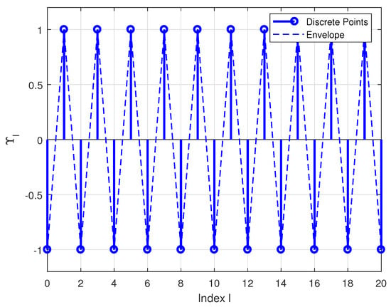
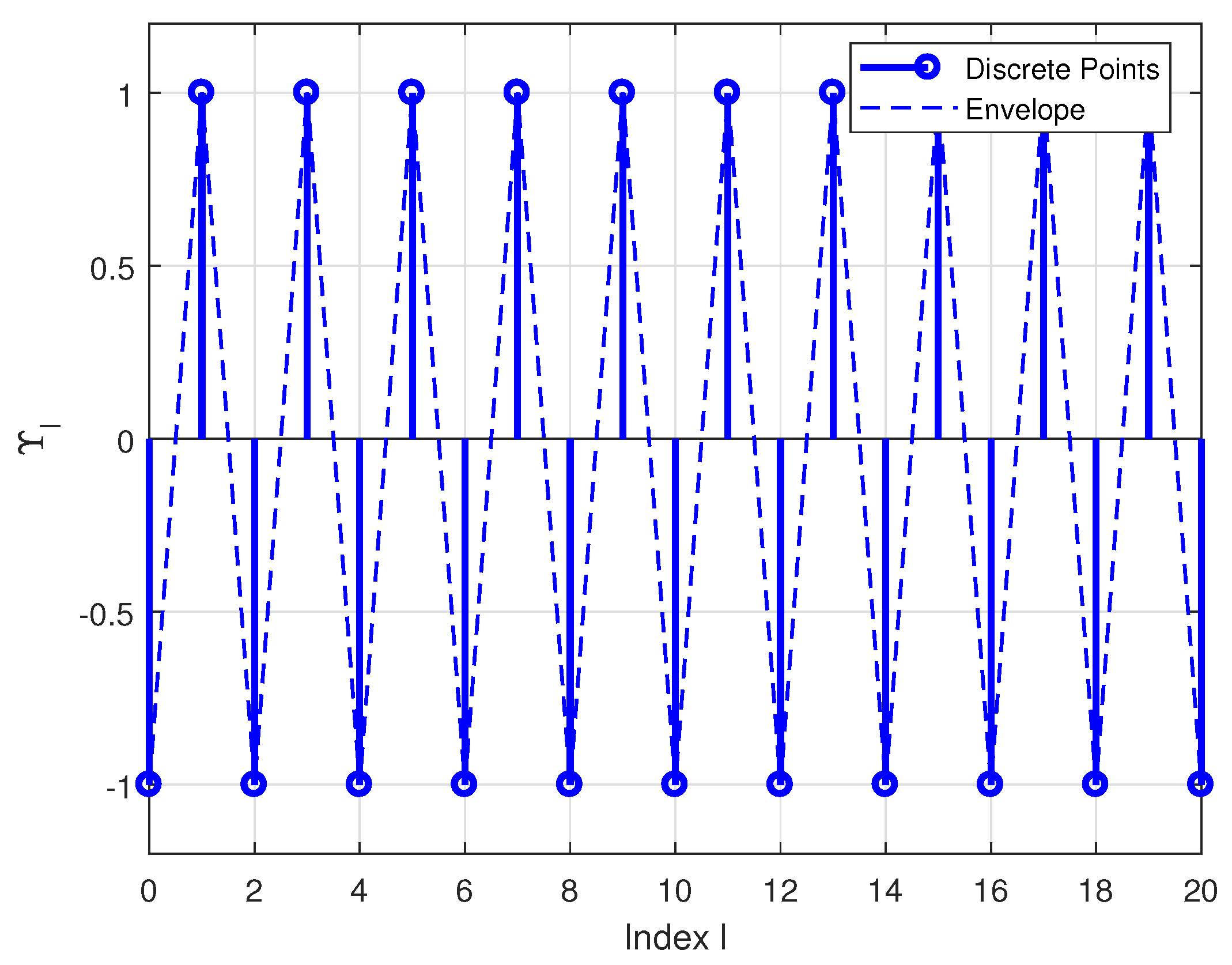
Then all the conditions of Theorem 1 are satisfied for (1). Hence, every solution of (1) oscillates.${\mathrm{Y}}_l={(-1)}^{l+1}$ is one such solution of (1). Figure 1 illustrates the oscillatory response of the nonlinear neutral delay difference equation characterized by a power of 5/3 nonlinearity. The solution ${\mathrm{Y}}_l={(-1)}^{l+1}$ displays a flawless alternating sequence of +1 and −1 within the index range $l\in [0,20]$, indicating that the suggested analytical solution adheres to the fractional powers and neutral delay terms, while the steady amplitude preservation corroborates the stability of the oscillatory behavior in the nonlinear domain.

Figure 1. Oscillatory response of neutral delay difference equations in Example 1.

Example 2.

Consider a neutral delay difference equation of second order, which has the form

$$\Delta \left[l^2\{\Delta ({\mathrm{Y}}_l+{\mathrm{Y}}_{l-2})\}\right]+4{(l+1)}^2{\mathrm{Y}}_{l-1}+4l^2{\mathrm{Y}}_{l-1}=0,$$

(55)

where $m_l=l^2,n_l=1,\sigma =\beta =\mu =1$, where $B_t=min\{p_l,p({\eta }_l)\}=4(l^2-2l+4)$, $A_l=min(q_l,q({\eta }_l))=4(l^2-2l+4)$.

$$\sum _{l=0}^{\infty }{\displaystyle \frac{1}{m_l}}<\infty ,$$

$$\sum _{s=l_0}^{\infty }\left[D_{\sigma }^{\mu }({\gamma }_s)B_s+D_{\sigma }^{\mu }({\tau }_s)A_s\right]$$

$$\sum _{s=l_0}^{\infty }\left[{\displaystyle \frac{1}{{(s-1)}^2}}4(l^2-2l+4)+{\displaystyle \frac{1}{{(s-1)}^2}}4(l^2-2l+4)\right]=\infty ,$$

and

$$\sum _{l=0}^{\infty }{\left[{\displaystyle \frac{1}{m_l}}\sum _{s=T}^{l-1}\left[D_{\sigma }^{\mu }({\gamma }_s)B_s+D_{\sigma }^{\mu }({\tau }_s)A_s\right]\right]}^{{\displaystyle \frac{1}{\mu }}}$$

$$\sum _{l=0}^{\infty }{\left[{\displaystyle \frac{1}{s^2}}\sum _{s=T}^{l-1}\left[{\displaystyle \frac{1}{{(s-1)}^2}}4(l^2-2l+4)+{\displaystyle \frac{1}{s^2}}4(l^2-2l+4)\right]\right]}^{{\displaystyle \frac{1}{\mu }}}=\infty ,T>0.$$

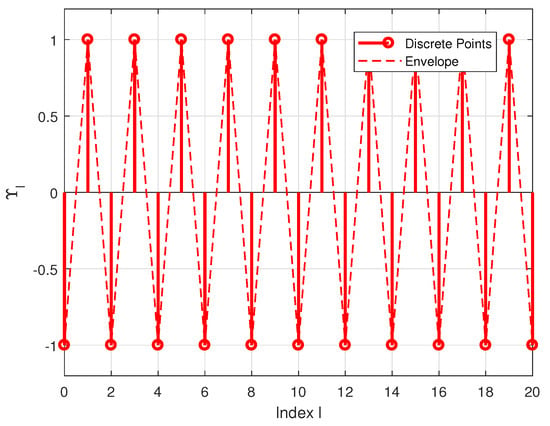
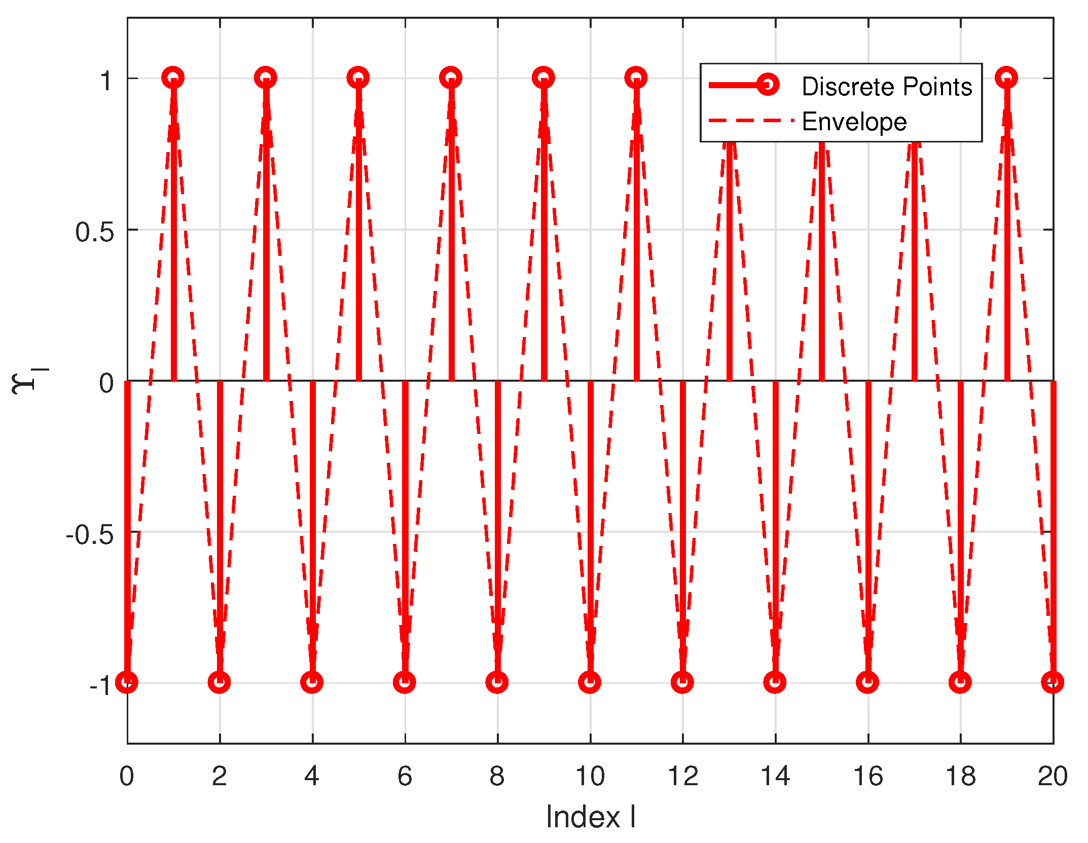
Then all the conditions of Theorem 8 are satisfied for (1). Hence, every solution of (1) oscillates.${\mathrm{Y}}_l={(-1)}^{l+1}$ is one such solution of (1). Figure 2 illustrates the response of the linear neutral delay difference equation, exhibiting a similar oscillating pattern ${\mathrm{Y}}_l={(-1)}^{l+1}$. The linear case, defined by quadratic coefficients and first-order differences, possesses the same fundamental solution as its nonlinear equivalent. This visual confirmation emphasizes the universality of the oscillatory mode across all problem types and demonstrates the resilience of the analytical method in addressing both linear and nonlinear neutral delay difference equations with uniform delay structures.

Figure 2. Oscillatory response of neutral delay difference equations in Example 2.

5. Conclusions

This paper analyzes the oscillation criteria for second-order neutral delay difference equations of the form

$$\Delta \left(m_l{\left(\Delta ({\mathrm{Y}}_l+n_l\mathrm{Y}({\eta }_l))\right)}^{\sigma }\right)+p_l{\mathrm{Y}}^{\beta }({\gamma }_l)+q_l{\mathrm{Y}}^{\mu }({\tau }_l)=0.$$

We assume that ${\sum }_{l=0}^{\infty }{\left({\displaystyle \frac{1}{m_l}}\right)}^{{\displaystyle \frac{1}{\sigma }}}=\infty$ or ${\sum }_{l=0}^{\infty }{\left({\displaystyle \frac{1}{m_l}}\right)}^{{\displaystyle \frac{1}{\sigma }}}<\infty$ for various ranges of $n_l$, where $\sigma$ is a quotient of odd positive integers. For the solution of second-order neutral delay difference equations, we develop new oscillation conditions. Some existing results for difference equations are extended and unified by our findings. Future work will focus on extending the present oscillation criteria to stochastic and probabilistic neutral difference equations, as well as developing control-based approaches for regulating oscillatory behavior in discrete-time systems, and also apply comparison techniques with second-order equations and explore oscillation conditions under more general nonlinearities and time-varying delays.

References

- Purushothaman, G.; Poornaval, S.; Chatzarakis, G.E.; Thandapani, E. Oscillation Criteria for hybrid second order neutral delay difference equations with mixed coefficients. Axioms 2025, 14, 571. [Google Scholar] [CrossRef] [Scilit]
- Chhatria, G.N. On Oscillatory second order impulsive neutral difference equations. AIMS Math. 2020, 5, 2433–2447. [Google Scholar] [CrossRef] [Scilit]
- Vidhyaa, K.S.; Thandapani, E.; Alzabut, J.; Ozbekler, A. Oscillation Criteria For Non-Canonical Second-Order Nonlinear Delay Difference Equations with A Superlinear Neutral Term. Electron. J. Differ. Equ. 2023, 2023, 1–12. [Google Scholar] [CrossRef] [Scilit]
- Banu, S.M.; Nalini, S. Oscillation of second order difference eqaution with several super linear neutral terms. Adv. Differ. Equ. 2018, 2018, 345. [Google Scholar] [CrossRef] [Scilit]
- Moaaz, O.; Al-Jaser, A. Monotonic and oscillatory features of solutions to general functional differential equations with a neutral-delay argument. Alex. Eng. J. 2025, 126, 546–554. [Google Scholar] [CrossRef] [Scilit]
- Agarwal, R.P. Difference Equations and Inequalities; Marcel Dekker: New York, NY, USA, 2000. [Google Scholar]
- Agarwal, R.P.; Bohner, M.; Grace, S.R.; O’Regan, D. Discrete Oscillation Theory; Hindawi: New York, NY, USA, 2005. [Google Scholar]
- Sethi, A.K. Oscillation of a functional differential equations of second order. Glob. J. Pure Appl. Math. 2017, 13, 5625–5634. [Google Scholar]
- Rehak, P. Oscillation and nonoscillation criteria for second order linear difference equations. Fasc. Math. 2001, 31, 71–90. [Google Scholar]
- Qian, C.; Ladas, G. Oscillation of First-Order Neutral Equations with variable coefficients. Monatshefte Math. 1990, 109, 103–111. [Google Scholar]
- Selvarangam, S.; Rupadevi, S.A.; Thandapani, E.; Pinelas, S. Existence of nonoscillatory solutions to third order neutral type difference equations with delay and advanced arguments. Math. Bohem. 2021, 146, 263–278. [Google Scholar] [CrossRef] [Scilit]
- Elaydi, S. An Introduction to Difference Equation; Springer: New York, NY, USA, 1996. [Google Scholar]
- Gyori, I.; Ladas, G. Oscillation Theory of Delay Differential Equations with Applications; Clarendon Press: Oxford, UK, 1991. [Google Scholar]
- Ganesh, P.; Palani, G.; Graef, J.R.; Thandapani, E. Oscillation of fourth order nonlinear semi-canonical neutral differnce equations via canonical Transformations. Abstr. Appl. Anal. 2024, 2024, 6682607. [Google Scholar] [CrossRef] [Scilit]
- Vimala, R.; Kodeeswaran, R.; Cep, R.; Krishnasamy, M.J.I.; Awasthi, M.; Santhakumar, G. Oscillation of nonlinear delay difference eqautions of fourth order. Mathematics 2023, 11, 1370. [Google Scholar] [CrossRef] [Scilit]
- Santra, S.S.; Majumder, D.; Bhattacharjee, R. Oscillation Tests: Second order neutral difference eqaution. In Proceedings of the Industry Interactive Innovations in Science, Engineering & Technology (I3SET2K19), Kolkata, India, 19–20 December 2019. [Google Scholar]
- Gomathi Jawahar, G.; Gopinath, P. Some properties of oscillation of second order neutral delay difference equations. Int. J. Dyn. Fluids 2017, 13, 47–51. [Google Scholar]
- Grace, S.R.; Graef, J.R. Oscillatory Behavior of second order nonlinear difference equations with a nonlinear nonpositive neutral term. Miskolc Math. Notes 2019, 20, 899–910. [Google Scholar] [CrossRef] [Scilit]
- Grace, S.R. Oscillatory Behavior of second order nonlinear difference equations with mixed Neutral terms. Boimed. J. Sci. Tech. Res. 2022, 47, 7522. [Google Scholar] [CrossRef] [Scilit]
- Grace, S.R. New Oscillation criteria of nonlinear second order delay difference equations. Mediterr. J. Math. 2022, 19, 166. [Google Scholar] [CrossRef] [Scilit]
- Bazighifan, O.; Chatzarakis, G.E. Oscillatory and Asymptotic behavior of advanced differential equations. Adv. Differ. Equ. 2020, 2020, 414. [Google Scholar] [CrossRef] [Scilit]
- Santra, S.S. Necessary and sufficient conditions for oscillation of second-order differential equation with several delays. Stud. Univ. Babes-Bolyai Math. 2023, 68, 319–330. [Google Scholar] [CrossRef] [Scilit]
- Tripathy, A.K.; Sethi, A.K. Sufficient conditions for oscillation and nonoscillation of a class of scond-order neutral differential equations. Adv. Dyn. Syst. Appl. 2018, 13, 73–90. [Google Scholar]
- Bolat, Y.; Gevgesoglu, M.; Chatzarakis, G.E. Oscillatory properties for emden—Fowler type difference equations with oscillating coefficients. Results Appl. Math. 2024, 23, 100472. [Google Scholar] [CrossRef] [Scilit]
- Yu, J.S.; Tang, X.H. Sufficient conditions for the oscillation of linear delay difference equations with oscillating coefficients. J. Math. Sci. 2000, 250, 735–742. [Google Scholar] [CrossRef] [Scilit]
- Baculikova, B.; Dzurina, J. Oscillation theorems for second order nonlinear neutral differential equations. Comput. Math. Appl. 2011, 62, 4472–4478. [Google Scholar] [CrossRef] [Scilit]
Disclaimer/Publisher’s Note: The statements, opinions and data contained in all publications are solely those of the individual author(s) and contributor(s) and not of MDPI and/or the editor(s). MDPI and/or the editor(s) disclaim responsibility for any injury to people or property resulting from any ideas, methods, instructions or products referred to in the content. |
© 2025 by the authors. Licensee MDPI, Basel, Switzerland. This article is an open access article distributed under the terms and conditions of the Creative Commons Attribution (CC BY) license (https://creativecommons.org/licenses/by/4.0/).