A Three-Machine Flowshop Scheduling Problem with Linear Fatigue Effect

Abstract

Highly customized requirements in smart manufacturing result in the unavoidable manual execution of complex operational procedures. Physical and mental fatigue from long work periods for assembly-line operators induces production issues, such as defective work-in-processes or equipment failure. An effective production schedule should account for worker fatigue. This study investigates a three-machine flowshop scheduling problem with the objective of makespan minimization, in which a linear fatigue effect function provides an approximate mathematical representation of fatigue and recovery processes in workers. A mixed integer programming (MIP) model is developed to optimize the integration of automated and human-operated production in manufacturing systems. Given its NP-hardness, an improved tabu search (ITS) algorithm is designed to obtain high-quality solutions, incorporating multiple initial solutions, a well-designed encoding-decoding strategy, and a tabu-based adaptive search mechanism to enhance efficiency. Numerical simulations indicate the veracity of the MIP model and the effectiveness of the ITS algorithm.

1. Introduction

The rapid development of information technology drives intellectualization in modern factories. Smart manufacturing saves human resources and improves production efficiency for enterprises. Customized production is one of the most essential characteristics of smart manufacturing [1]. Highly customized requirements in smart manufacturing result in the unavoidable manual execution of complex operational procedures [2]. For example, Jinko Solar Co., Ltd., has large-scale production lines for manufacturing solar panels. Manual quality inspection (MQI) requires that the inspector stochastically select solar panel units to verify quality standard or conduct supplementary checks for the units to find the potential issues that are ignored by automatic checks. The immediate predecessor and successor of the MQI operations are, respectively, automatic detection (performing basic quality testing for all products) and sorting procedures (classifying products into different categories), both of which are executed automatically.

These sequential operations constitute a three-stage flowshop production system, necessitating coordinated optimization between the intermediate manual process and adjacent automated stages to enhance overall operational efficiency. For the quality sampling operation, prolonged working hours may induce both physical and mental fatigue among sampling personnel, resulting in increased defect rates in work-in-process. A suitable implement of rest intervals enables effective recovery of strength and energy for tired workers. This phenomenon is recognized as fatigue effect in production [3]. Therefore, an optimal production scheduling system should account for worker fatigue while enhancing operational efficiency. This productive scenario is modeled as a three-machine flowshop scheduling problem with fatigue effect on the middle machine. This setting represents a typical human–machine collaborative scenario, in which the manual stage bridges two automated processes, allowing for the focused analysis of fatigue-related scheduling interactions without introducing unnecessary system complexity. For in-depth analysis of problem characteristics, a linear fatigue function provides an approximate mathematical representation of fatigue and recovery processed in workers. A mixed-integer programming (MIP) model is developed to optimize the integration of automated and human-operated production in manufacturing systems. Given the strong NP-hardness of the classical three-machine flowshop scheduling problem with the makespan criterion [4], the proposed fatigue-effect flowshop scheduling (FEFS) model inherits at least equivalent computational complexity. Specifically, the FEFS problem can be reduced from the classical flowshop scheduling problem by treating the worker fatigue parameters as additional time-dependent constraints, which further enlarges the feasible search space. Consequently, the problem remains NP-hard and cannot be solved optimally in polynomial time unless P = NP.

Considering this computational intractability, exact optimization methods such as branch-and-bound or mixed-integer linear programming are only applicable to small-scale instances and become impractical for large-scale industrial environments that require timely scheduling decisions. Therefore, this study adopts a metaheuristic framework to obtain high-quality near-optimal solutions within reasonable computation times. Tabu search (TS) is employed as the core optimization framework because its adaptive memory mechanism and neighborhood-based search strategy provide an effective balance between intensification and diversification, enabling efficient exploration of complex, nonlinear solution spaces. Furthermore, the inherent flexibility of TS allows the incorporation of problem-specific neighborhood operators, making it particularly suitable for handling the coupled decisions of job sequencing and rest-point placement under dynamic fatigue effects.

For large-scale production cases, an improved tabu search (ITS) algorithm is developed by integrating multiple initial-solution generation, a tabu-based adaptive search mechanism, and specialized neighborhood operators to further enhance convergence efficiency and robustness. Numerical experiments verify the correctness of the MIP model and demonstrate the superior performance of the proposed ITS algorithm.

2. Literature Survey

The integration of human fatigue into production scheduling has gained increasing attention as industries strive to enhance work quality and reduce economic losses. Montoya-Torres et al. [5] reviewed scheduling studies incorporating human factors such as fatigue, emphasizing that most formulations optimize makespan and total completion time. Building upon this foundation, several studies have modeled fatigue in diverse operational contexts. Lin et al. [6] addressed a multi-objective nurse rostering problem, introducing a linear weighting method to balance fatigue with scheduling preferences. Frank et al. [7] developed a fatigue-avoidance model for medical staff to mitigate fatigue accumulation under different shift patterns, aiming to improve efficiency and reduce the risk of medical errors. Zachary et al. [8] examined fatigue in long-distance truck driving, constructing a fatigue-aware model that ensures driver alertness remains within an acceptable range. Nayeri et al. [9] explored fatigue and priority constraints in emergency rescue scheduling, where the objectives focused on minimizing weighted completion time and tardiness.

A significant step toward analytical modeling was made by Li et al. [3], who proposed a single-machine scheduling model with exponential fatigue and recovery functions. Their work provided an important theoretical framework for understanding the interplay between fatigue and rest. However, the study was confined to a single operator and depended on simple heuristics, limiting its scalability to larger or human–machine collaborative systems. Akerstedt et al. [10] examined fatigue among short-haul flight crews, targeting the reduction in fatigue levels and improvement in sleep quality and task allocation. Likewise, Asadayoobi et al. [11] investigated firefighter scheduling by integrating fatigue, learning, and stress, optimizing both task duration and execution quality. Paredes-Astudillo et al. [12] analyzed a flowshop problem combining learning and fatigue, focusing on minimizing total completion time and cumulative fatigue dose per worker. Xu and Hall [13] later provided a comprehensive review summarizing the evolution of fatigue-aware personnel scheduling and identifying key opportunities for integrating operational research methods with human-centric design.

More recent studies have expanded fatigue modeling into multi-machine and human-centric scheduling environments. Berti et al. [14] examined a dual-resource constrained job-shop problem by incorporating worker heterogeneity, such as age and experience, developing mathematical and heuristic approaches to jointly optimize productivity and worker well-being. In the same vein, Aribi et al. [15] formulated a human-centric double flexible job shop scheduling problem with explicit fatigue constraints and proposed an improved decomposition-based multi-objective evolutionary algorithm to balance makespan and fatigue-induced errors. Within hybrid flowshop contexts, Marichelvam et al. [16] considered learning and forgetting effects and presented an improved particle swarm optimization method combining NEH and variable neighborhood search strategies. Paredes-Astudillo et al. [17] employed a multi-agent simulation framework to assess how alternative break policies affect worker fatigue and system performance. Vermin et al. [18] incorporated predictive fatigue models into cobotic order-picking systems, proposing a bi-objective MINLP to jointly minimize makespan and energy expenditure. Similarly, Usman and Lu [19] integrated ergonomic factors such as workload and human energy expenditure into a flexible job shop and designed a multi-objective discrete Jaya algorithm to achieve balanced optimization. Ostermeier [20] explored unpaced mixed-model assembly lines, defining a processing-time function that captures learning, forgetting, fatigue, and recovery, demonstrating its impact on various scheduling objectives through simulation analysis.

In summary, scheduling research incorporating fatigue has evolved from conceptual and single-resource analyses to complex, multi-machine human-centric systems. However, critical methodological gaps remain in terms of model generality, algorithm adaptability, and empirical verification: (1) most existing models are limited to small-scale or simulation-based settings and lack tractable formulations that jointly represent fatigue and recovery dynamics; (2) although some studies incorporate multiple machines, they seldom emphasize the interaction between humans and automated equipment, whereas real production systems often involve human participation only in specific stages, making such human–machine coupling crucial; (3) many heuristic and metaheuristic methods are problem-specific and lack adaptive mechanisms for broader generalization; and (4) few works conduct rigorous statistical testing, leaving the robustness of their results uncertain.

The present study addresses these challenges by developing a mixed-integer programming formulation that explicitly models fatigue and recovery in a three-machine human–machine flowshop, and by proposing an improved tabu search (ITS) algorithm with adaptive memory and multiple neighborhood structures. Statistical tests are further conducted to verify the optimizer’s superiority. This integrated approach not only extends existing fatigue-aware scheduling literature but also provides a more practical and generalizable framework for enhancing production reliability and efficiency.

3. Problem Description

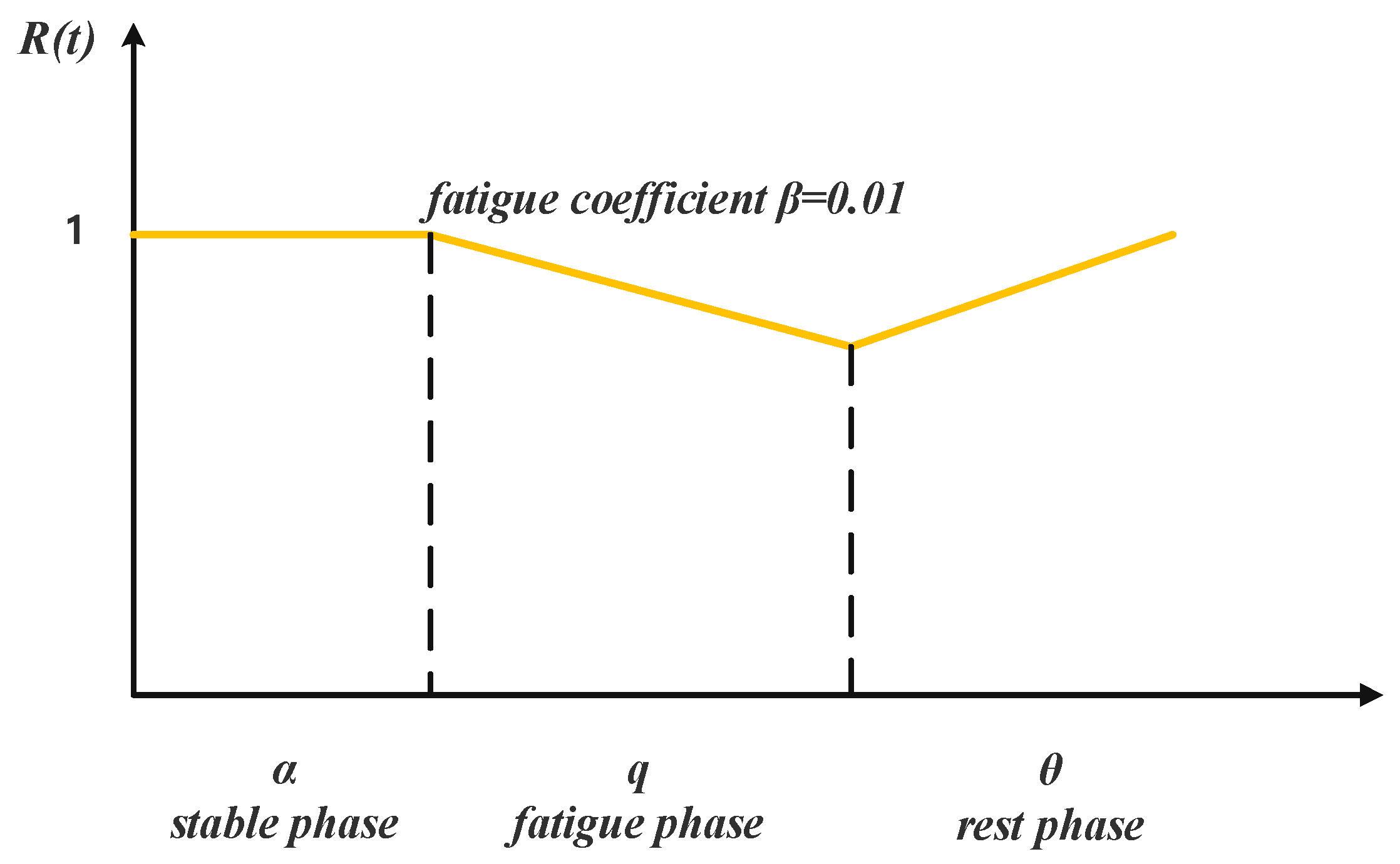
The investigated TFEFS problem consists of three processing stages, with the middle stage operated by a human, while the first and third stages are automated. The processing of n jobs follows a sequential order from stage 1 to stage 3. At any given time, each stage can process at most one job, and no job can be processed by more than one stage simultaneously. Once a job starts processing, it cannot be interrupted. The operation O_ij represents job j being processed at stage i, where i = 1, 2, 3; 1 ≤ j ≤ n. The processing time p_ij denotes the standard operation time for operation O_ij. In the second stage, the worker’s process can be described as ‘stable period—work efficiency decay (fatigue)—rest.’ As illustrated in Figure 1, during the initial α period, the worker experiences a stable efficiency level where their efficiency remains constant at 1, referred to as the work adaptation period. After this stable period, work efficiency begins to decline due to fatigue, following a linear degradation model. In the final θ period, the worker rests, leading to some recovery of their fatigue and a subsequent restoration of work efficiency.

Figure 1. Worker efficiency graph.

The production efficiency is modeled using a linear fatigue effect function. Initially, the worker operates at full efficiency, and the actual processing time p_ij for operation O_ij is simply the standard time. However, once the worker’s efficiency falls below 1, the actual processing time is recalculated. Let R(t) represent the worker’s efficiency at time t, and the job’s start time is t₁ (known), with the end time being t₂ (unknown), the relationship between work efficiency and processing time is given by ${\int }_{t_1}^{t_2}R$ = p_ij.

3.1. MIP Model

The relevant notations and the mathematical model are summarized below:

$M$	Set of machines $\left\{1, 2, 3\right\}$
$N$	Set of jobs $\left\{1, 2,\dots ,n\right\}$
$K$	Set of positions $\left\{1, 2,\dots ,n\right\}$
$\mathrm{Y}$	A very large positive constant
$p_{i,j}$	Normal processing time of job j on machine i
$p_{i,k}^p$	Processing time at position k on machine i
$\mathsf{\alpha }$	Duration of the worker’s stable period
$\mathsf{\beta }$	Efficiency decay coefficient during the fatigue period
$\mathsf{\theta }$	Duration of the rest period
$X_{j,k}$	$\left\{\begin{array}{c}1, \mathrm{i}\mathrm{f} \mathrm{j}\mathrm{o}\mathrm{b} j \mathrm{i}\mathrm{s} \mathrm{t}\mathrm{h}\mathrm{e} k-\mathrm{t}\mathrm{h} \mathrm{t}\mathrm{o} \mathrm{b}\mathrm{e} \mathrm{p}\mathrm{r}\mathrm{o}\mathrm{c}\mathrm{e}\mathrm{s}\mathrm{s}\mathrm{e}\mathrm{d}\\ 0,\mathit{else}\end{array}\right.$
$b_k$	$\left\{\begin{array}{c}1, \mathrm{if} \mathrm{the} \mathrm{worker} \mathrm{rests} \mathrm{after} \mathrm{the} k \mathrm{th} \mathrm{position}\\ 0,else\end{array}\right.$
$C_{max}$	Makespan (maximum completion time)
$S_{k,i}$	Start time at position k on machine i
$C_{k,i}$	Completion time at position k on machine i
$t_j^s$	Stable period processing time for the j-th job in the second stage
$t_j^w$	Fatigue period processing time for the j-th job in the second stage
$W_j^s$	Accumulated working time before processing the j-th job in the second stage
$W_j^e$	Accumulated working time after processing the j-th job in the second stage

Based on these notations, the MIP model is established as follows:

Minimize

$$C_{max}=max{C}_{k,3},k\in N$$

(1)

Subject to

$$\sum _{i=1}^n{b}_i=1$$

(2)

$$\sum _{j=1}^n{X}_{j,k}=1, k\in K$$

(3)

$$\sum _{k=1}^n{X}_{j,k}=1,j\in J$$

(4)

$$C_{k,1}=S_{k,1}+\sum _{j=1}^n\left(p_{1,j}\times X_{j,k}\right),k\in K$$

(5)

$$S_{k,1}\ge C_{k-\mathrm{1,1}},k\in K-\left\{1\right\}$$

(6)

$$p_{2,k}^p=\sum _{j=1}^n\left(p_{2,j}\times X_{j,k}\right),k\in K$$

(7)

$$W_k^s=0,k\in \left\{1\right\}$$

(8)

$$W_k^s=\left(1-b_{k-1}\right)\times W_{k-1}^e,k\in K-\left\{1\right\}$$

(9)

$$W_k^e=W_k^s+t_k^s+t_k^w,k\in K$$

(10)

$$\mathsf{\alpha }-W_k^s\ge -Y\times \left(1-z_k\right),k\in K$$

(11)

$$\mathsf{\alpha }-W_k^s\le Y\times z_k,k\in K$$

(12)

$$t_k^s\le z_k\times \left(\mathsf{\alpha }-W_k^s\right),k\in K$$

(13)

$$t_k^w\ge p_{2,k}^p-t_k^s,k\in K$$

(14)

$$t_k^s+t_k^w-0.5\times \mathsf{\beta }\times {\left(t_k^w\right)}^2=p_{2,k}^p,k\in K$$

(15)

$$C_{k,2}=S_{k,2}+t_k^s+t_k^w,k\in K$$

(16)

$$S_{k,2}\ge C_{k,1},k\in K$$

(17)

$$S_{2,k}\ge C_{2,k-1}+\mathsf{\theta }\times b_{k-1},k\in K-\left\{1\right\}$$

(18)

$$C_{k,3}=S_{k,3}+\sum _{j=1}^n\left(p_{3,j}\times X_{j,k}\right),k\in K$$

(19)

$$S_{3,k}\ge C_{2,k}$$

(20)

$$S_{3,k}\ge C_{3,k-1}$$

(21)

Constraint (1) defines the optimization objective of minimizing the makespan. Constraint (2) restricts the worker to taking only one rest during the processing. Constraints (3) and (4) ensure that each job is executed exactly once. Constraint (5) determines the completion time of each job at its corresponding position in the first stage. Constraint (6) establishes the job sequencing rules for the first stage. Constraint (7) formulates the actual processing time at the k th position in the second stage. Constraints (8)–(10) track the cumulative working time in the second stage. Constraints (11)–(13) confine the stable period processing time at the k th position to the remaining available stable duration. Constraint (14) limits the lower bound of the fatigue period time. Constraint (15) is derived from solving an integral and imposes a restriction on the actual completion time. Constraints (16)–(18) specify the processing sequence in the second stage. Constraints (19)–(21) regulate the processing sequence in the third stage.

From a computational perspective, the model involves O(n²) binary variables X_j,k for job-position assignments and O(n) binary variables b_k for rest-point decisions. The factorial growth of the feasible space renders exact optimization impractical for medium- and large-scale instances.

3.2. A Scheduling Instance

To illustrate the problem more clearly, a six-job instance is presented. The processing times are listed in Table 1, and the worker’s three state durations and fatigue coefficient are set as α = 3, β = 0.01, and θ = 5, respectively, as depicted in Figure 1. The optimal processing sequence is J₅-J₄-J₂-J₆-J₃-J₁, resulting in the makespan of 68.02. The corresponding Gantt chart is shown in Figure 2.

Table 1. Job processing times.

	${\mathit{J}}_1$	${\mathit{J}}_2$	${\mathit{J}}_3$	${\mathit{J}}_4$	${\mathit{J}}_5$	${\mathit{J}}_6$
$p_1$	10	8	9	11	7	10
$p_2$	5	6	4	7	5	6
$p_3$	8	7	9	6	10	8

Figure 2. Gantt chart for the instance.

4. Iterated Tabu Search Algorithm

Tabu Search (TS) is a global optimization algorithm based on neighborhood search [21,22]. Its fundamental mechanism involves maintaining a tabu list that records recently visited local optima [23]. By prohibiting the revisiting of these solutions, the algorithm effectively avoids cycling and thereby escapes local traps [24]. To prevent the exclusion of potentially promising moves, an aspiration criterion is introduced: a tabu move is accepted if it yields a solution superior to the current best. In this context, the objective function value serves as the fitness metric, with smaller values representing higher-quality solutions.

The investigated problem is NP-hard, making exact optimization methods unfeasible for medium- and large-scale instances. Although many metaheuristic algorithms could be applied, TS is particularly suitable for this problem due to two key features: (1) TS employs a memory-based mechanism that prevents cycling and reduces the chance of revisiting inferior solutions, which is effective in handling such complexity. (2) The fatigue effect introduces dynamic changes in worker efficiency that easily lead to local optima. TS balances intensification and diversification during the search process, enabling the algorithm to escape local traps while still exploiting promising regions. These characteristics make it more suitable than evolutionary algorithms, which often converge prematurely when dealing with fatigue-driven variability [25].

To further adapt TS to the fatigue-aware scheduling environment, this study proposes an improved iterated tabu search (ITS) that incorporates multi-initial solution generation, well-designed encoding-decoding method, tabu-adaptive strategy and variable neighborhood exploration, which together enhance solution quality and stability for large-scale instances.

4.1. Encoding and Decoding

The TFEFS problem involves a strong coupling between job sequencing decisions and rest-point arrangements. This coupling significantly increases complexity of the solution space, making the design of an appropriate encoding–decoding method essential for optimization.

4.1.1. Encoding Method

The encoding scheme must not only represent the processing order of jobs, as in classical flowshop scheduling problems, but also incorporate the timing of worker rest-point in order to capture the dynamic transitions between stable, fatigue, and recovery states. Such a representation allows the algorithm to accurately model the interaction between human factors and machine operations. Based on this principle, two complementary encoding methods are introduced, namely, job sequence encoding and rest point encoding.

(1)

Job Sequence Encoding:

An integer permutation is used to represent the processing order of jobs. For a problem with n jobs, a feasible job sequence π can be represented as a vector of length n: $\pi =\left({\pi }_1,{\pi }_2,\dots ,{\pi }_n\right)$, where π_k is the number of the k th job to be processed, $k\in \left\{\mathrm{1,2},\dots ,n\right\}$. This encoding method intuitively represents the processing sequence of jobs on the flow line.

(2)

Rest Point Encoding:

To determine the timing of the worker’s rest, we introduce the rest point as an independent decision variable in the encoding. $k_r$ is an integer representing the insertion of a rest between the processing of the ${(k}_r-1$) th job and the $k_r$th job. The value range of ${ k}_r$ is $\left\{1,2,\dots ,n\right\}$, where $k_r=1$ means resting before any job starts (equivalent to starting from a fully rested state), and $k_r=k \left(k>1\right)$ indicates resting after job ${\pi }_{k-1}$ is completed and before job ${\pi }_k$ begins. Therefore, a complete solution (individual) can be represented by a tuple (π, $k_r$). This encoding method, which explicitly separates the job sequence and the rest point, allows for the design of neighborhood operations targeting different decision variables in subsequent optimization algorithms (like Tabu Search), thus exploring the solution space more effectively.

4.1.2. Decoding Method

The decoding procedure is designed to evaluate the quality of a candidate solution by calculating its makespan based on the given job sequence $\pi =\left({\pi }_1,{\pi }_2,\dots ,{\pi }_n\right)$ and the selected rest point $k_r$. This process follows the three-stage flowshop structure and translates the encoded decision variables into actual start and completion times while incorporating the effects of fatigue and recovery.

(1)

Completion Time Calculation

Stage 1. This stage involves pure machine processing, and its calculation follows standard flow-shop rules. As shown in Pseudocode 1, the first job in the sequence starts at time 0, and its completion time equals its processing duration. The subsequent job begins immediately after the previous one finishes, and its completion time is obtained by adding its processing time.

Stage 2. This stage models the human operator’s work cycle, consisting of a stable period, a fatigue period, and a recovery period. The operator’s cumulative working time determines whether they are in the stable period or the fatigue period. The process is described as follows.

Pseudocode 1: Completion Time Calculation (Stage 1)
1	Start
2	$S_{1,1}\leftarrow 0$ // Initialize start and completion time
3	$C_{1,1}\leftarrow S_{1,1}+p_{1,{\pi }_1}$
4	For k from 2 to n do
5	$S_{1,1}\leftarrow C_{1,k-1}$
6	$C_{1,k}\leftarrow p_{1,{\pi }_k+}{S}_{1,k}$
7	End

Pseudocode 2: Completion Time Calculation with Fatigue Effect (Stage 2)
1	Start
2	Initialize cumulative working time to 0
3	For k ← 1 to n do //Iterate through jobs starting from the first
4	// Step 1: Determine the start time of the current job
5	If $k=r$ then //If the current position is the planned rest point
6	$S_{2,k} \leftarrow max\{C_{2,k-1}+\theta ,C_{1,k}\}$//Start time must account for rest duration
7	Reset cumulative working time to zero after rest
8	Else
9	$S_{2,k} \leftarrow max\{C_{2,k-1},C_{1,k}\}$//Normal flow-shop rule
10	Cumulative working time ← Cumulative working time from the previous round
11	// Step 2: Calculate actual processing time based on fatigue effect
12	If job is processed entirely within the stable period α
13	$p_{2,{\pi }_k}^{’}\leftarrow p_{2,{\pi }_k}$
14	Else if job processing spans the stable and fatigue periods
15	$p_s\leftarrow \mathrm{c}\mathrm{u}\mathrm{m}\mathrm{u}\mathrm{l}\mathrm{a}\mathrm{t}\mathrm{i}\mathrm{v}\mathrm{e} \mathrm{p}\mathrm{r}\mathrm{o}\mathrm{c}\mathrm{e}\mathrm{s}\mathrm{s}\mathrm{i}\mathrm{n}\mathrm{g} \mathrm{t}\mathrm{i}\mathrm{m}\mathrm{e}$
16	$p_f\leftarrow p_{2,{\pi }_k}-p_s$
17	${\delta }_f \leftarrow$calculate based on fatigue formula $\left(p_f\right)$
18	$p_{2,{\pi }_k}^{’} \leftarrow p_s+{\delta }_f$
19	Else //Job is processed entirely within the fatigue period
20	$p_{2,{\pi }_k}^{’} \leftarrow$calculate based on fatigue formula $\left(p_{2,{\pi }_k}\right)$
21	End if
23	// Step 3: Update completion time and cumulative working time
24	$C_{2,k}\leftarrow S_{2,k}+p_{2,{\pi }_k}^{’}$
25	Cumulative working time
26	End for
27	End

Stable Period: If the cumulative working time does not exceed the threshold α, the worker operates at full efficiency, and the processing time for the job remains the same as the standard time p.

Fatigue Period: When the cumulative working time exceeds α, the worker’s efficiency decreases due to fatigue, resulting in extended processing times. The decline in efficiency is represented by a linear fatigue function. Jobs that span both the stable and fatigue periods require the calculation of both the standard processing time in the stable period and the extended processing time in the fatigue period. This is calculated by solving the following quadratic equation:

$$0.5\beta t^2-t+p=0$$

where β represents the fatigue decay coefficient, p is the standard processing time, and t denotes the time required to complete the task in the fatigued state. The actual processing time δ_f is calculated as the smaller real root of this equation.

As described in Pseudocode 2, the actual processing time for a job in Stage 2 is thus determined by combining the stable time p_s and the fatigue time p_f based on the fatigue model.

Stage 3. Due to the problem constraints, the processing of a job in the third stage cannot begin until it has been completed in the second stage. For each subsequent job, its start time must satisfy two conditions: (1) the machine in the third stage must be available (i.e., the previous job has finished processing), and (2) the job itself must have completed its second-stage processing. Therefore, its start time is calculated as follows:

S_3,k = max (C_{3,k − 1}, C_2,k).

Pseudocode 3: Completion Time Calculation
1	Start
2	$S_{\mathrm{3,1}}$←$C_{\mathrm{2,1}}$//Initialize start and completion time
3	$C_{\mathrm{3,1}}$←$S_{\mathrm{3,1}}+p_{3,{\pi }_1}$
4	for k from 2 to n do
5	$S_{3,k}$←$max\left\{C_{3,k-1},C_{2,k}\right\}$
6	$C_{3,k}$←$p_{3,{\pi }_k+}{S}_{3,k}$
7	End

The completion time is obtained by adding the processing time in Stage 3. The detailed process is summarized in Pseudocode 3.

(2)

Decision on Completion Time

For a given job sequence π, its fitness value is determined by its optimal rest strategy, which plays a crucial role in minimizing the makespan. Unlike traditional scheduling problems, where the objective function depends solely on job sequence, this problem requires iterating through all possible rest points $k_r\in \left\{1,2,\dots ,n\right\}$ to evaluate the impact of different rest timings on the overall performance. Each rest point corresponds to a unique makespan $C_{max}(\pi ,k_r)$, reflecting how the worker’s fatigue and recovery influence the completion times across all stages of the flowshop. The optimal makespan for a job sequence π is obtained by selecting the rest point that results in the smallest value:

$$C_{max}={min}_{k_r\in \{1,\dots , n\}}\left\{C_{max}\right(\pi ,k_r\left)\right\}$$

Once the optimal makespan is determined, the rest point that minimizes this value is identified as the optimal rest point $k_r^{*}\left(\mathsf{\pi }\right)$:

$$k_r^{*}\left(\pi \right)=\mathit{arg}{min}_{k_r\in \{1,\dots , n\}}\left\{C_{max}\right(\pi ,k_r\left)\right\}$$

The decoding procedure converts the job sequence π and the optimal rest point k(π) into actual completion times across the three stages. This method not only ensures feasibility but also accurately models the complexities of human–machine collaboration. The proposed encoding–decoding strategy serves as a foundation for the ITS algorithm, enabling it to handle the dynamic nature of fatigue in the scheduling process. This approach combines traditional scheduling principles with a sophisticated model of worker dynamics, contributing to more efficient optimization strategies.

4.2. Initial Population

The design of high-quality initial solutions is crucial to the performance of the ITS algorithm, since the search space is strongly influenced by the dual decision variables of job sequence and rest point. To address this, a heuristic-based initialization is proposed, combining greedy rules with randomization to balance solution quality and diversity.

Step 1. Processing times from the three stages are integrated into a weighted index. Jobs with longer processing times are prioritized for scheduling within the stable period, since this allocation reduces the likelihood of excessive delays in the fatigue period. To achieve this, weights are assigned to the three stages, and a weighted sum is calculated as the priority index for each job. Jobs are then sorted in descending order of this index to construct a greedy-based initialization sequence.

Step 2. To improve population diversity, multiple random permutations of jobs are also generated and incorporated into the initial solutions. The position r is obtained using a random strategy, which allows the ITS algorithm to explore a wide range of rest-point placements during the search process. This hybridization ensures that both high-quality heuristic solutions and exploratory random solutions are available, reducing the risk of premature convergence.

Step 3. The solutions generated from Steps 1–2 are combined to form the initial population.

Pseudocode 4: Initial Population
1	Start
2	For each job j∈{1, …, n} do
3	// Step 1: Calculate weighted priority index
4	wj ← w1·p1,j + w2·p2,j + w3·p3,j
5	End for
6	Sort jobs in descending order of wj
7	Construct greedy-based job sequence πg = (π1, π2, …, πn)
8	Add solution (πg, r) into initial population
9	// Step 2: Generate additional random sequences
10	For j = 1 to rand do
11	Generate random permutation πrand
12	Generate random rest point rrand∈{1, …, n}
13	Add solution (πrand, rrand) into initial population
14	End for
15	// Step 3: Combine greedy and random solutions
16	Return initial population {(π, r)}
17	End

Overall, the initialization phase is not only responsible for producing feasible starting points but also plays a critical role in ensuring that the ITS algorithm can effectively exploit fatigue-aware characteristics. The combination of heuristic prioritization, weighted evaluation, and randomized diversification lays the groundwork for robust performance in subsequent optimization. The detailed process is presented in Pseudocode 4.

4.3. Tabu-Based Adaptive Search Mechanism

4.3.1. Problem-Specific Search Operators

In the proposed ITS algorithm, the design of search operators is critical for effectively exploring the solution space. Insertion and swap operators are designed to efficiently explore the solution space by adjusting the job sequence while considering worker fatigue and recovery. These operators have been proven to be highly effective in flow shop scheduling, with low computational complexity, making them suitable for large-scale problems [26].

(1)

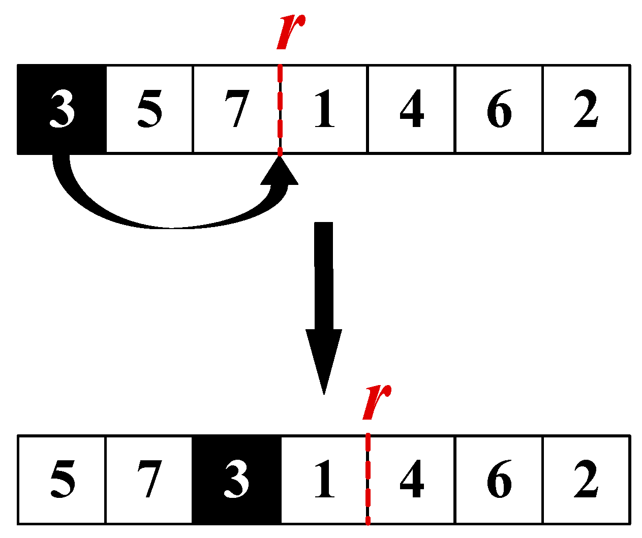
Insertion with Rest Adjustment

A job is removed from its current position and inserted into a new one. After the insertion, the rest point is slightly adjusted so that heavy jobs are less likely to cluster in the fatigue period. As shown in Figure 3, this operator allows the algorithm to rebalance workload and reduce the makespan.

Figure 3. Example of Operator o₁: remove J₃ and place it between J₇ and J₁.

Step 1: Select job j from sequence π.

Step 2: Remove job j from its current position and insert it into a new position.

Step 3: Adjust the rest point r slightly to balance workload before and after the rest.

Step 4: Recalculate the makespan under the new configuration.

(2)

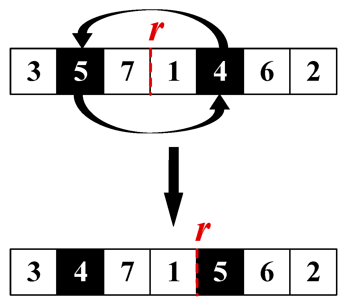
Swap with Rest Adjustment

Two jobs exchange their positions in the sequence. Once swapped, the rest point is shifted nearby to keep the balance between the stable and fatigue periods. As illustrated in Figure 4, this operator tests alternative local orderings while respecting fatigue recovery.

Figure 4. Example of Operator o₂: swap the positions of J₅ and J₄.

Step 1: Select two jobs J_a and J_b from the sequence.

Step 2: Swap the positions of J_a and J_b.

Step 3: Shift the rest point r locally to adapt to the new order.

Step 4: Recalculate the makespan under the updated sequence.

(3)

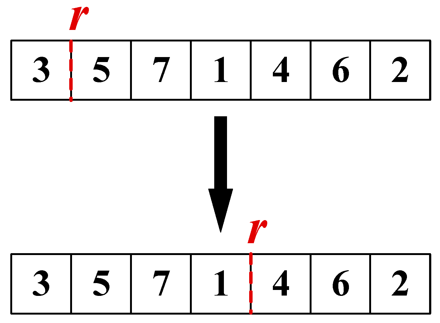
Rest Point Relocation

The rest point itself is moved a few positions forward or backward, without changing the job order. This operation directly explores how different rest placements affect overall completion time, helping the algorithm avoid getting trapped in poor rest configurations. An example is provided in Figure 5.

Figure 5. Example of Operator o₃: relocate rest point r between J₁ and J₄.

Step 1: Keep the current job sequence π unchanged.

Step 2: Move the rest point r a few positions forward or backward.

Step 3: Recalculate the makespan under the new rest placement.

(4)

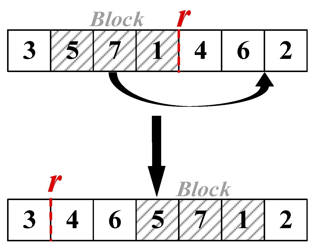
Block Perturbation

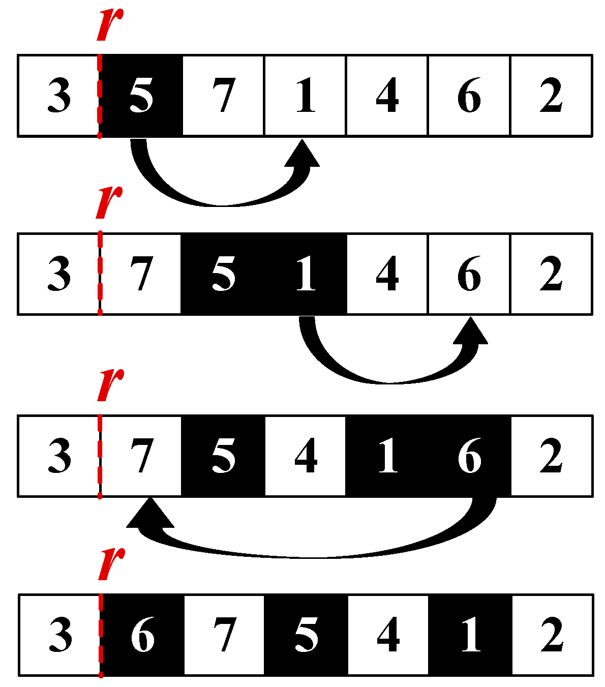
A small block of consecutive jobs is moved to a new position, especially across the rest point. This helps reorganize workload distribution on both sides of the rest period (Figure 6).

Figure 6. Example of Operator o₄: insert block between J₆ and J₂.

Step 1: Select a block of consecutive jobs {J_a, …, J_b} from sequence π.

Step 2: Remove the block from its original position.

Step 3: Insert the block into a new position crosses the rest point.

Step 4: Recalculate the makespan for the new configuration.

Pseudocode 5: Tabu-based Adaptive Search Mechanism
1	Start
2	Initialize tabu list T = ∅
3	For i from 1 to 30 do
4	// Step 1: Evaluate each operator
5	For each oi∈O do
6	Generate candidate moves from oi
7	For each move
8	If not tabu
9	Keep it
10	Else
11	Keep only if it improves the best global
12	End if
13	End for
14	Select the one with the best makespan
15	Record its improvement Δi
16	End for
17	// Step 2: Select operator
18	Choose operator o* that maximizes ($S_i-\partial P_i$)
19	Update solution x, and insert move attributes into tabu list
20	// Step 3: Update scores and frequency
21	For each oi∈O do
22	Si ← (1 − λ) Si + λΔi
23	End for
24	Update frequency counters
25	// Step 4: Update tabu list
26	Decrease tenure of all tabu attributes and remove expired ones
27	End for
28	End

(5)

Chain Ejection

Starting from a job near the rest point, a chain of jobs is sequentially removed and reinserted into new positions. This creates larger changes in the sequence and avoids local stagnation. Figure 7 illustrates this process for better comprehension.

Figure 7. Example of Operator o₅: Chain for J₅, J₁ and J₆.

Step 1: Select a job J_s close to the rest point as the starting job.

Step 2: Remove J_s and insert it into a new position.

Step 3: Eject the displaced job and reinsert it into another position, repeating the chain for a limited number of steps.

Step 4: Adjust the rest point r to align with the new sequence structure.

Step 5: Recalculate the makespan after the chain operation.

Together, these operators provide a balance between local adjustments (insertion, swap, rest-shift) and larger-scale changes (block relocation, chain insertion). By combining them, the algorithm can flexibly explore diverse neighborhoods while maintaining the fatigue-recovery mechanism.

4.3.2. Tabu-Adaptive Strategy

To dynamically balance exploitation and diversification, an adaptive operator selection strategy is incorporated into the ITS framework. Let O = {o₁, …, o₅} denote the five operators. For each operator o_i, a performance score S_i is maintained and updated according to its recent contribution:

S_i ← (1−λ)S_i + λΔi

where Δ_i represents the improvement in makespan achieved by operator o_i in the latest iteration (Δi = 0 if no improvement occurs), and λ∈(0, 1) is a learning rate controlling score sensitivity. To avoid overusing a single operator, a frequency penalty P_i is also recorded as the number of times o_i has been applied in the recent sliding window.

At each iteration, the operator is chosen by the following equation:

$$o^{*}=arg\underset{\mathit{oi}\in O}{\max }(S_i-\mathit{\partial }{P}_i)$$

where $\partial$ is a penalty coefficient. Tabu restrictions are enforced by discarding forbidden moves unless aspiration criteria are met.

Tabu restrictions are enforced by discarding any candidate move whose attributes (e.g., the moved job, and the rest-point shift) appear in the tabu list. Such a move can only be accepted if it satisfies the aspiration criterion, i.e., it produces a solution strictly better than the current global best. The detailed process is summarized in Pseudocode 5.

4.4. Framework

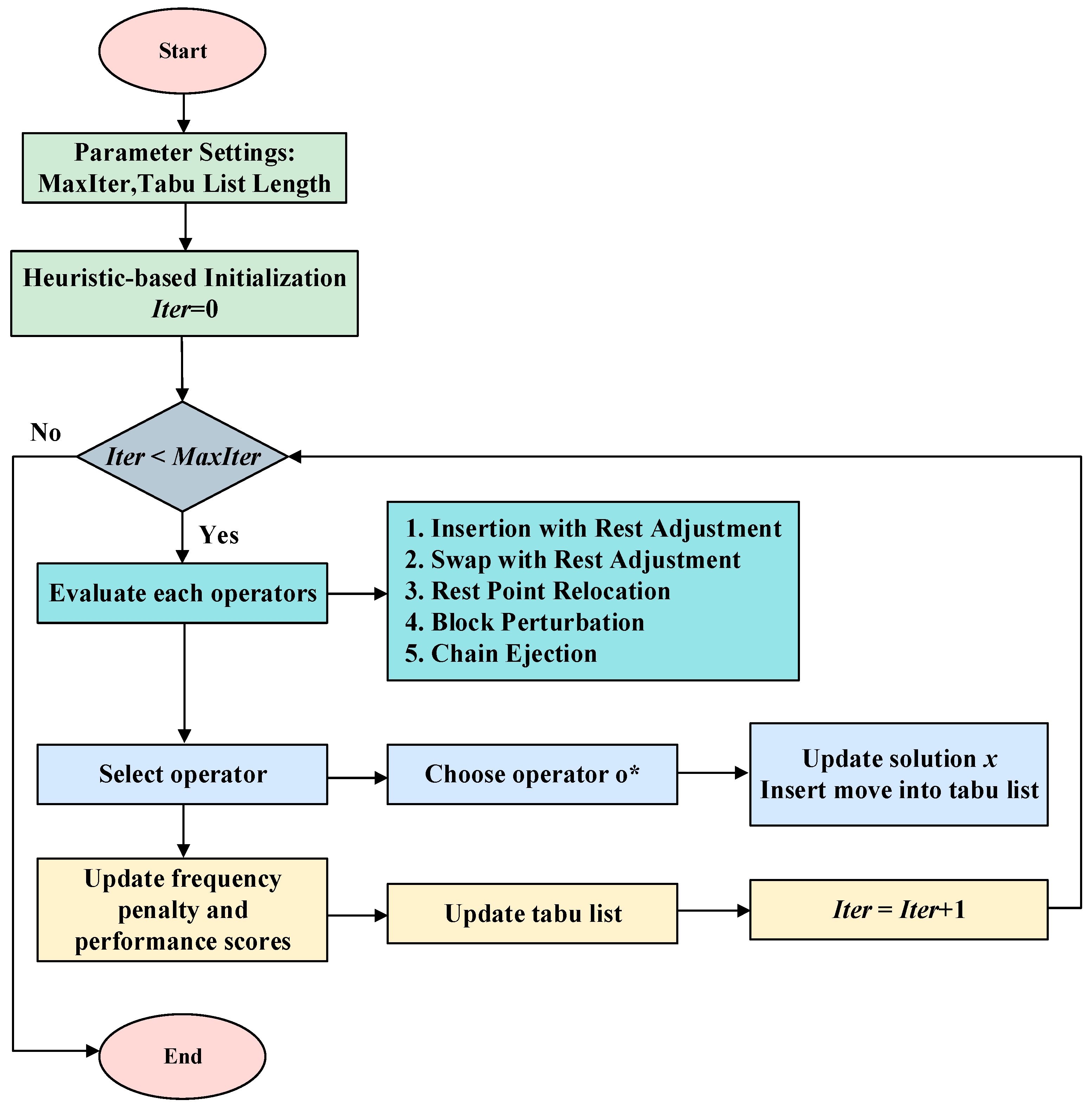
This section provides a comprehensive summary of the proposed ITS algorithm, detailing its framework. The following steps outline the algorithm’s structure, from the generation of initial solutions to the final optimization process. Additionally, the corresponding flowchart (Figure 8) visually represents the sequential flow of the algorithm, highlighting the interactions between the different phases.

Figure 8. Flowchart of the ITS algorithm.

Step 1. Initialization: A diverse set of initial solutions is generated through a hybrid approach combining greedy heuristics and randomization to ensure both solution quality and population diversity.

Step 2. Encoding and Decoding: The problem is encoded by separately representing the job sequence and worker rest points. The decoding process evaluates the makespan based on the given sequence and rest-point configuration.

Step 3. Tabu Search: A TS mechanism is employed to explore the solution space, utilizing memory structures to avoid revisiting previously explored solutions and escape local optima.

Step 4. Adaptive Search: An adaptive strategy is incorporated to dynamically select search operators, adjusting exploration and exploitation based on the performance of each operator during the search.

Step 5. Termination: The algorithm terminates after a predefined number of iterations.

5. Experimental Analysis

To comprehensively evaluate the effectiveness of the proposed ITS algorithm, a series of experiments were conducted, covering parameter calibration, comparative evaluation, optimizer benchmarking, and component analysis. Two advanced intelligent optimization algorithms, Differential Evolution (DE) [27] and Genetic Algorithm (GA) [28], were selected as baselines. All algorithms share the same encoding–decoding framework to ensure fairness. The following subsections describe the experimental design, conditions, and results in detail.

5.1. Experimental Conditions and Settings

To ensure the reliability and reproducibility of the evaluation, the experimental conditions were carefully designed from four perspectives: fatigue effect settings, problem scale, processing time generation, and computational environment. These settings were derived based on empirical data provided by enterprises in the industrial robotics and intelligent manufacturing sector, ensuring that the experiments reflect realistic fatigue–recovery cycles observed under typical operational conditions. The details are presented as follows.

(1)

Fatigue Effect Settings:

The worker fatigue model was parameterized as follows: stable period duration α = 100, rest duration θ = 30, and the linear slope of efficiency decay β = 1/170. These settings allow the experiments to reflect realistic fatigue–recovery cycles.

(2)

Test Scale

The investigated problem contains three stages (two machine-operated and one human-operated stages). The number of jobs was set to four scales: 50, 100, 150, and 200.

(3)

Processing Time Data

For each instance, processing times were sampled from a uniform distribution U(20, 70). The datasets were pre-generated and stored externally to guarantee reproducibility across algorithms.

(4)

Experimental Environment

All algorithms were implemented in C++ and executed on a workstation equipped with an Intel i7-6700 CPU (3.4 GHz, 8 cores) and 24 GB of memory.

These settings establish a controlled and reproducible environment for large-scale testing.

5.2. Orthogonal Experiment

To avoid biased parameter settings, a comprehensive orthogonal design of experiments was carried out for each algorithm. Following the Taguchi method, the MIR (Mean Improvement Rate) was recorded for each factor combination:

$$MIR={\displaystyle \frac{Z_f-Z_i}{Z_i}}\times 100\%$$

where Z_i denotes the initial objective value under a given parameter setting, and Z_f represents the best objective value obtained. A higher MIR value indicates a greater improvement. The main effect plots were illustrated to identify optimal parameter levels. The calibration was performed on instances of 50 jobs with 3 machines, ensuring comparability across methods.

5.2.1. Improved Tabu Search Algorithm

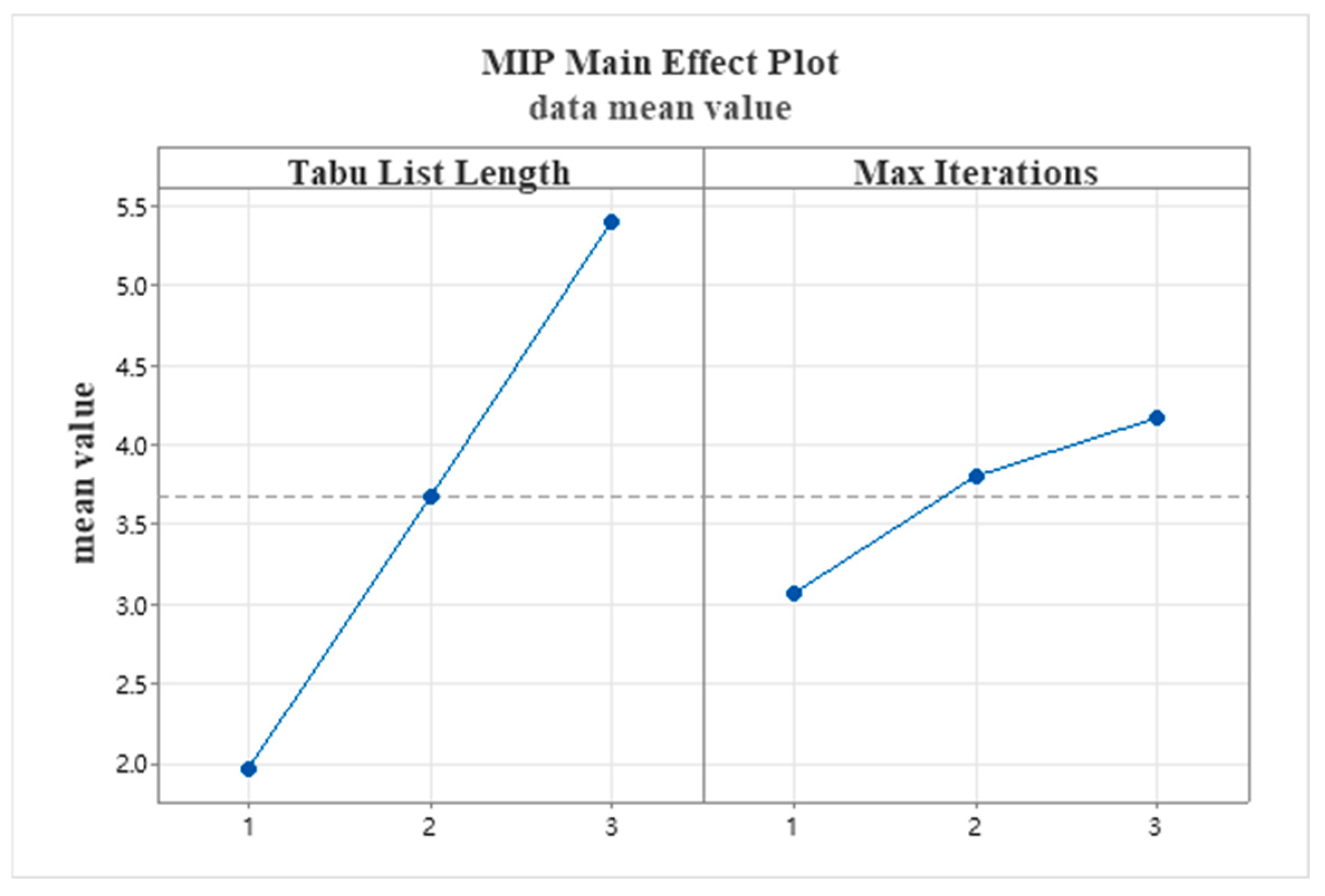
To determine the optimal parameter combination for the ITS algorithm, this section conducts an orthogonal experiment on its key parameters: tabu list length and maximum number of iterations. As shown in Table 2, three levels were set for each of these two parameters. The results for the MIR values under different parameter combinations are detailed in Table 3. The main effect plot drawn from the experimental results (Figure 9) shows that the MIR value is optimal when both the tabu list length and the maximum number of iterations are at level 3. Therefore, the final parameters adopted for the ITS algorithm are as follows: a tabu list length of 7 and a maximum of 300 iterations.

Table 2. Tabu Search Algorithm Factor Level Table.

Level	Tabu List Length	Max Iterations
1	3	100
2	5	200
3	7	300

Table 3. Tabu Search Algorithm Orthogonal Experiment MIR Values.

Tabu List Length	Max Iterations	MIR
1	1	1.5
1	2	2.3
1	3	2.1
2	1	3.1
2	2	3.4
2	3	4.5
3	1	4.6
3	2	5.7
3	3	5.9

Figure 9. Tabu Search Main Effect Plot.

Although the achieved MIR values are relatively small (below 6%), this phenomenon can be reasonably explained. All algorithms were implemented under the same encoding–decoding framework, which ensures fair comparison but also makes the baseline performance of the compared methods relatively strong, leaving limited space for further improvement. Moreover, the efficient encoding–decoding strategy and heuristic-based initialization employed in this study produce high-quality initial solutions, thereby narrowing the measurable improvement margin. Nevertheless, the proposed ITS algorithm consistently achieves the best results with lower variance across all parameter combinations, demonstrating superior stability and robustness.

5.2.2. Differential Evolution

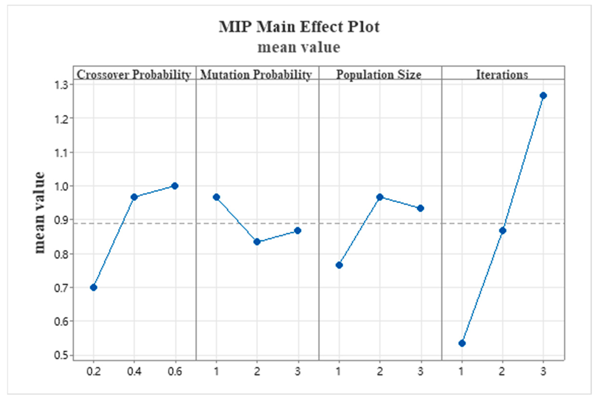
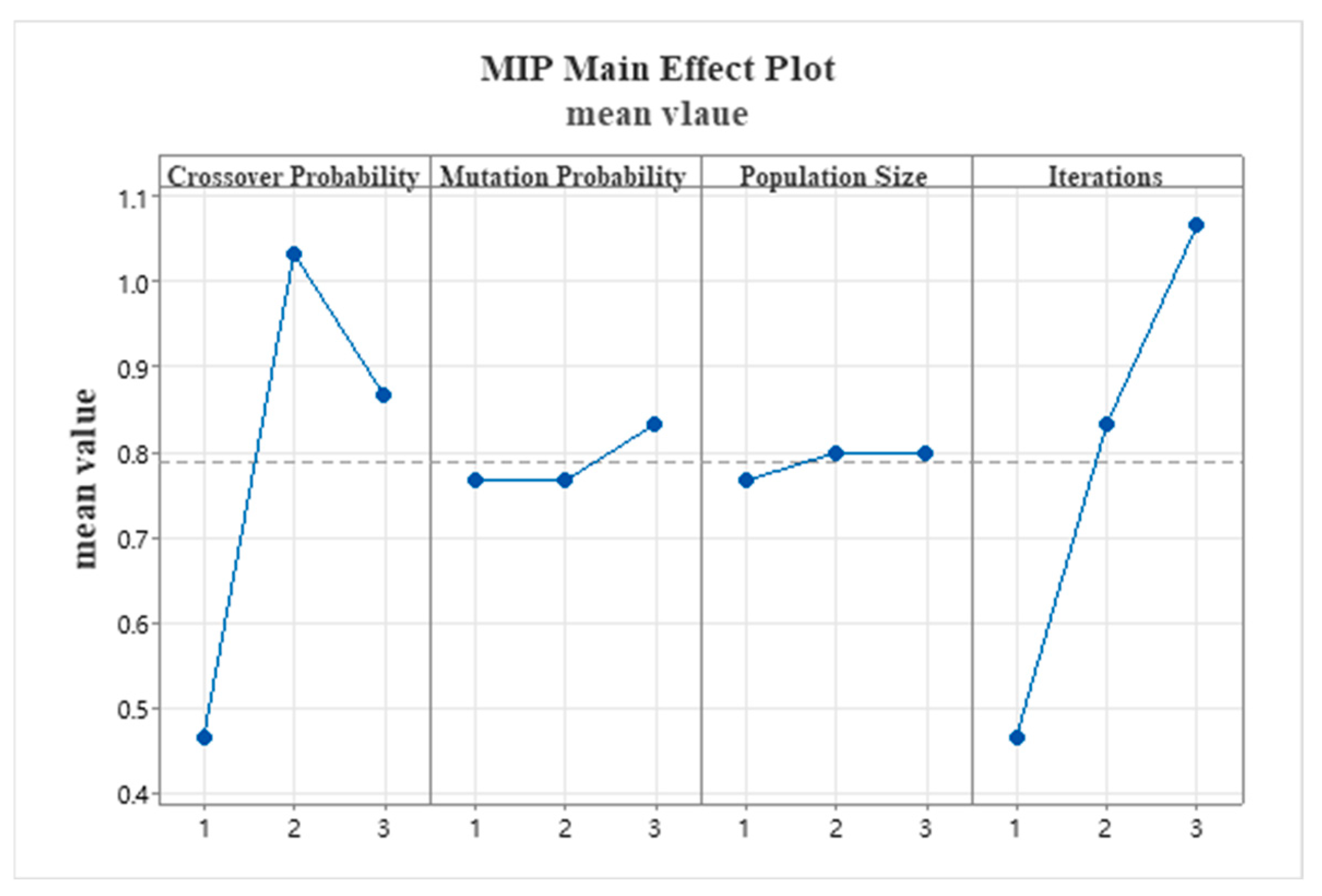
To determine the optimal parameter combination for the DE algorithm, this section shows an orthogonal experiment on its core parameters: crossover probability, mutation probability, population size, and maximum number of iterations. The experiment adopts the factors and levels shown in Table 4, and the corresponding MIR values under different parameter settings are listed in Table 5. Based on the main effect plot of the results (Figure 10), the best performance is achieved when the crossover probability is 0.4, the mutation probability is 0.6, the population size is 100, and the maximum number of iterations is 300. Accordingly, these values are selected as the final parameter settings of the DE algorithm.

Table 4. Parameter Combinations for DE and GA.

Level	Crossover Probability	Mutation Probability	Population Size	Max Iterations
1	0.2	0.2	50	100
2	0.4	0.4	100	200
3	0.6	0.6	150	300

Table 5. Orthogonal Experiment MIR Values for DE.

Crossover Probability	Mutation Probability	Population Size	Iterations	MIR
0.2	1	1	1	0.3
0.2	2	2	2	0.7
0.2	3	3	3	1.1
0.4	1	2	3	1.5
0.4	2	3	1	0.6
0.4	3	1	2	0.8
0.6	1	3	2	1.1
0.6	2	1	3	1.2
0.6	3	2	1	0.7

Figure 10. Main Effect Plot for DE.

5.2.3. Genetic Algorithm

To determine the optimal parameter combination for GA, this section presents an orthogonal experiment on its core parameters: crossover probability, mutation probability, population size, and maximum number of iterations, with the factors and levels shown in Table 4. The MIR values obtained under different parameter combinations are listed in Table 6. Based on the main effect plot of the experimental results (Figure 11), the optimal settings are identified as crossover probability 0.4, mutation probability 0.6, population size 100, and maximum iterations 300, which are thus adopted as the final GA parameters.

Table 6. Orthogonal Experiment MIR Values for GA.

Crossover Probability	Mutation Probability	Population Size	Iterations	MIR
1	1	1	1	0.1
1	2	2	2	0.5
1	3	3	3	0.8
2	1	2	3	1.3
2	2	3	1	0.7
2	3	1	2	1.1
3	1	3	2	0.9
3	2	1	3	1.1
3	3	2	1	0.6

Figure 11. Main Effect Plot for GA.

5.3. Comparative Experiment

To verify the effectiveness of the proposed algorithm, this section presents a comparative experiment for analysis. Relative Percentage Deviation (RPD) is used as the evaluation metric, which is calculated as follows:

$$RPD={\displaystyle \frac{X_a-X_{min}}{X_{min}}}\times 100\%$$

where X_a represents the objective value of an algorithm, and X_min represents the minimum value among all results.

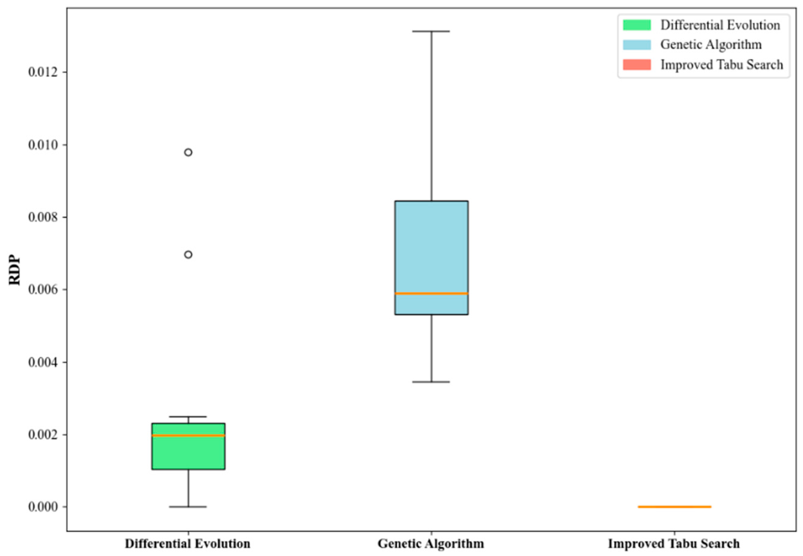
Table 7 details the RPD results for the three algorithms for problem instances of different scales. In all 12 instances across all tested scales (from 50 to 200 jobs), the RPD value for the proposed ITS algorithm is consistently 0. This indicates that ITS was able to find a solution equal to or better than the best solution found by the other compared algorithms in every run, demonstrating its excellent optimization capability and stability. Although DE and GA were also able to find feasible solutions, their RPD values were all greater than 0, indicating that their solution quality was generally inferior to that of ITS. For example, in the second instance with 50 jobs, the RPD value of GA was as high as 1.312, showing a significant gap between its solution quality and the best solution. These two population-based evolutionary algorithms are more prone to getting stuck in local optima when faced with the complex solution space of the investigated problem.

Table 7. Algorithm Comparison Results (RPD values).

Number of Jobs	DE	GA	ITS
50	0.697	0.658	0
	0.111	1.312	0
	0.008	0.899	0
100	0.979	0.409	0
	0.086	0.631	0
	0.000	0.826	0
150	0.203	0.550	0
	0.225	0.545	0
	0.192	0.345	0
200	0.226	0.523	0
	0.249	0.534	0
	0.142	0.967	0

The box plot in Figure 12 shows that the ITS algorithm consistently achieves an RPD value of 0, forming a flat horizontal line. This result highlights both its superior performance and remarkable stability. In contrast, the box plots of DE and GA exhibit higher medians, indicating poorer performance. Such fluctuations suggest that DE and GA are less robust and prone to unstable solution quality. In summary, the results of the comparative experiment strongly validate the effectiveness and superiority of the ITS algorithm proposed in this study for solving the investigated problem with fatigue effects.

Figure 12. Box Plot of Comparative Experiment Results.

To further verify the statistical significance of ITS’s performance advantage, both paired t-tests and Wilcoxon signed-rank tests were conducted on the RPD results. The p-values for the paired t-tests were 0.0049 (DE vs. ITS) and 1.52 × 10⁻⁶ (GA vs. ITS), while the corresponding p-values for the Wilcoxon tests were 0.00049 and 0.00024, respectively. All values are well below the 0.05 significance level, confirming that the performance improvements of ITS over DE and GA are statistically significant. These results provide strong evidence that the superiority of ITS is not due to random variation but reflects a consistent and significant improvement in solution quality.

Furthermore, an analysis of the rest-point placement reveals a consistent behavioral pattern of the fatigue-aware scheduling mechanism. Across all tested scales (50–200 jobs), the optimal rest point tends to occur in the mid-to-late part of the sequence, typically between 45% and 70% of the total processing order. This pattern indicates that the algorithm naturally schedules rest after a substantial workload has accumulated, reflecting realistic fatigue progression among workers. The slight backward shift of the rest point as the job size increases suggests that under heavier workloads, longer continuous operation before rest becomes beneficial for minimizing makespan, as it balances efficiency loss and recovery gains.

5.4. Optimizer Comparison

This section evaluates the performance of the proposed ITS algorithm against a state-of-the-art commercial solver, Gurobi 11.0, in order to identify the applicable problem scales for each method. Test instances were generated with job sizes ranging from 6 to 1000, and the maximum computation time was limited to 10 min.

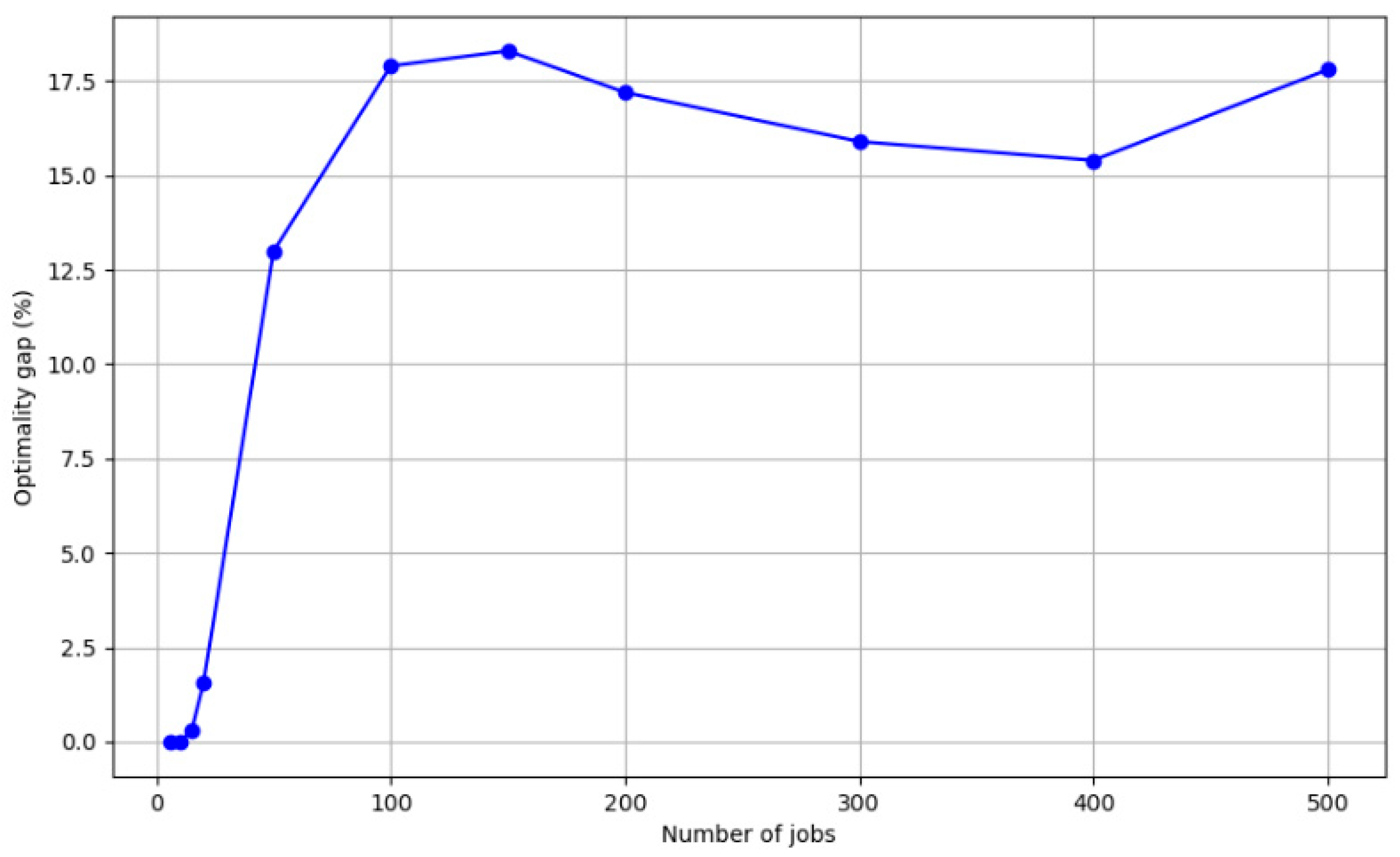
For small-scale problems (6 and 10 jobs), Gurobi achieved a gap of 0.0%, indicating convergence to the global optimum. ITS obtained the same results within 1 s, demonstrating comparable accuracy with negligible runtime. Figure 13 illustrates the variation in Gurobi’s optimization gap as problem size increases. It is evident that, from 15 jobs onward, Gurobi fails to converge to an optimality gap of 0 (e.g., Gap = 0.31% at 15 jobs), and the gap widens further as the problem size grows. This suggests that, for medium- to large-scale instances, Gurobi struggles to guarantee optimality within the given time limit.

Figure 13. Gurobi Solver Gap Values.

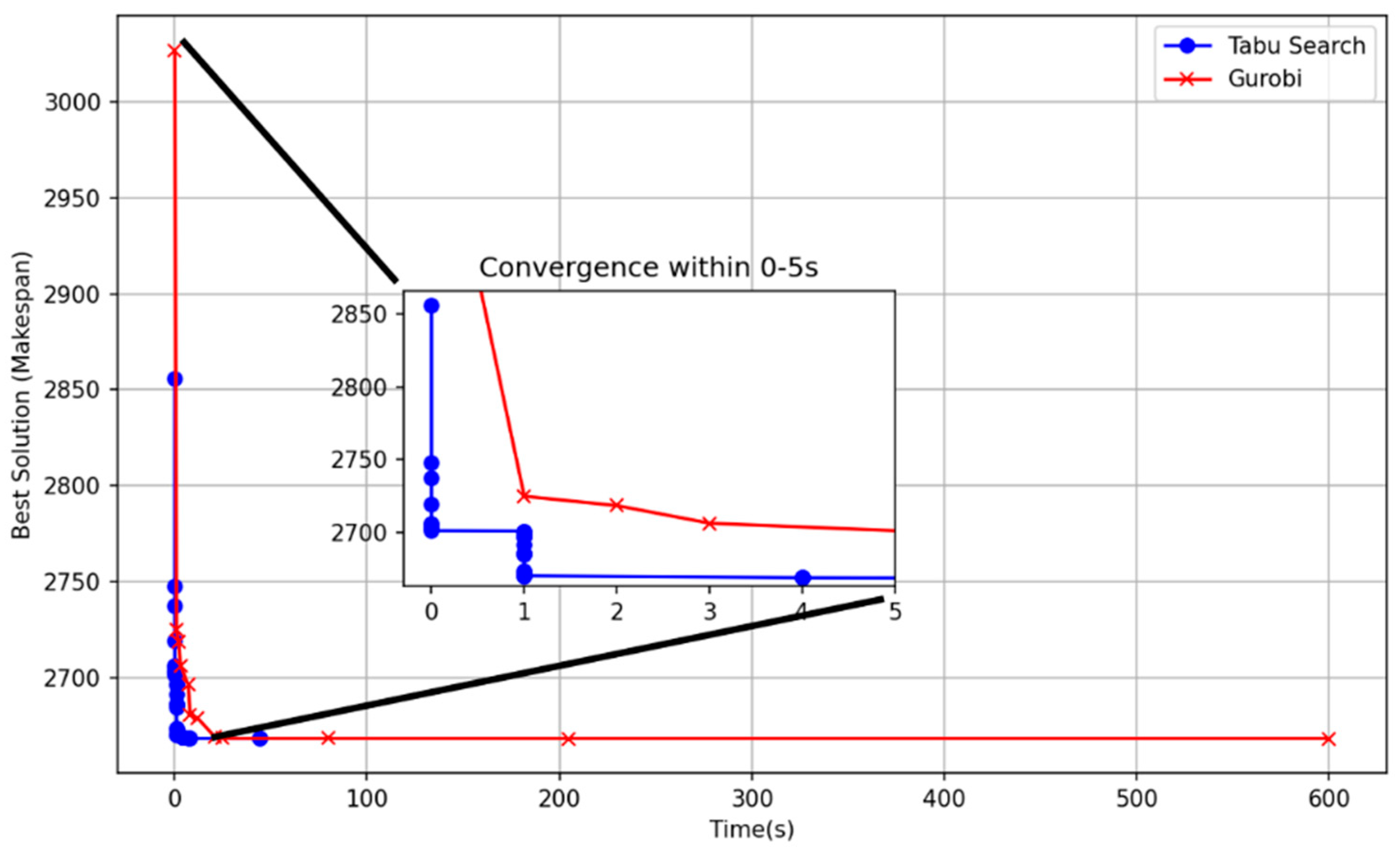
For problem sizes below 200 jobs, ITS and Gurobi generally yielded identical solutions. However, ITS exhibited a much faster convergence speed. As shown in Figure 14 for the 50-job case, ITS, benefitting from heuristic initialization and efficient neighborhood search, rapidly converged to the optimum, whereas Gurobi improved only gradually. This demonstrates the superior convergence efficiency of the ITS algorithm.

Figure 14. Convergence Comparison Chart.

For large-scale problems (exceeding 200 jobs), ITS consistently outperformed Gurobi in both solution quality and runtime. Table 8 reports detailed comparisons, showing that ITS not only produced better solutions but also required significantly less time. For example, in the 300-job instance, ITS reached a superior solution in 42 s, while Gurobi required 600 s and still returned a weaker result. These findings confirm that, when dealing with complex large-scale scheduling problems, the ITS algorithm is more effective and efficient than the advanced commercial solver.

Table 8. Optimal Solution Comparison.

Number of Jobs	ITS		Gurobi		RPD
	Best Solution	Time (s)	Best Solution	Time (s)
200	10,868.641	10	10,880.958	600	0.1133
300	16,178.460	42	16,186.516	600	0.0499
400	21,583.300	315	21,608.150	600	0.1153
500	27,360.297	126	27,407.431	600	0.1718

5.5. Component Analysis Experiment

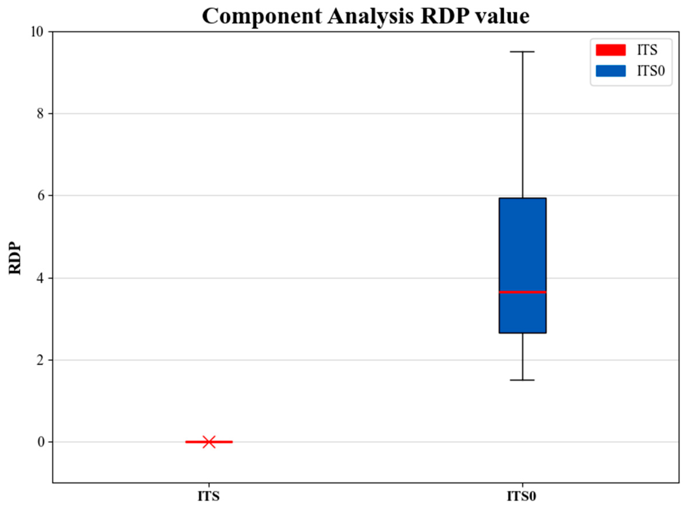
To validate the effectiveness of the tabu-based adaptive search mechanism, a component analysis experiment was conducted. The complete ITS algorithm was compared with a reduced version referred to as ITS0, where tabu-based adaptive search mechanisms were removed and the search relied only on simple neighborhood moves. This comparison quantifies the contribution of the designed operators to overall algorithmic performance.

The results, summarized in Table 9, show that the complete ITS achieved the best solutions in all tested instances, with RPD values consistently equal to 0. In contrast, ITS0 produced inferior results in most cases, with positive RPD values across different problem scales. This clearly indicates that, without the tabu-based adaptive search mechanism and problem-specific operators, the search process cannot adequately explore the solution space, leading to poorer solution quality.

Table 9. Component Analysis Results (RPD values).

Number of Jobs	ITS	ITS0
50	0	2.8
	0	3.0
	0	1.5
100	0	7
	0	2.2
	0	5.1
150	0	7.2
	0	5.6
	0	3.5
200	0	9.5
	0	2.0
	0	3.8

Figure 15 further illustrates these findings from a statistical perspective. The box plot for ITS collapses into a horizontal line at RPD = 0, reflecting both superior optimization capability and remarkable robustness across repeated runs. By contrast, the box plot for ITS0 exhibits higher medians, indicating weaker average performance and significant instability.

Figure 15. Component Analysis Results Box Plot.

To further confirm the reliability of these observations, statistical significance analyses were carried out on the RPD values of ITS and ITS0. Both a paired t-test and a Wilcoxon signed-rank test were performed. The obtained p-values were 3.30 × 10⁻⁵ for the paired t-test and 0.00024 for the Wilcoxon test. In both cases, the p-values are well below the conventional 0.05 significance threshold, providing strong statistical evidence that the performance improvement of ITS over ITS0 is highly significant. This component analysis confirms that the use of problem-specific operators is essential for the performance of the ITS algorithm. Their absence results in a substantial loss of search efficiency and robustness, highlighting that the operators are not generic heuristics but carefully designed mechanisms that exploit the structural characteristics of the fatigue-aware flowshop scheduling problem.

5.6. Fatigue Modeling Assessment

In this section, we conducted a direct performance comparison between models with and without fatigue modelling. The gap value is calculated as follows:

$$gap={\displaystyle \frac{C_{max}^{no\_fatigue}-C_{max}^{fatigue}}{C_{max}^{no\_fatigue}}}\times 100\%$$

From Table 10, we observe that, for small instance sizes (≤50 jobs), the gap is slightly negative (−0.42%), indicating that introducing rest points slightly degraded makespan in that regime. However, as the number of jobs increases, the gap steadily turns positive and grows (e.g., 2.01% improvement at 400 jobs). This trend is consistent with intuitive expectations: when the workload is light, fatigue does not accumulate significantly, so modelling rest may even introduce overheads; when the workload becomes large, fatigue accumulation may degrade performance enough that explicitly modelling rest yields measurable improvements.

Table 10. Comparison of gap values between fatigue-aware and non-fatigue models.

Job-machine	50	100	150	200	250	300	350	400
Gap value (%)	−0.42	0.03	0.26	0.87	0.95	1.01	1.46	2.01

From an industrial perspective, the results imply that fatigue modelling becomes increasingly relevant in high-volume, large-scale production scenarios. Moreover, beyond pure makespan optimization, incorporating human fatigue aligns with the broader agenda of human-centered manufacturing. The literature in ergonomics and workforce scheduling underscores that human factors such as fatigue and recovery can influence throughput and safety. In summary, although the absolute improvement in makespan may appear modest, the consistent positive trend for larger instances combined with the human-centric benefits justifies the inclusion of fatigue modelling for scalable and sustainable production systems.

6. Conclusions

This study addressed the three-stage flow-shop scheduling problem with explicit consideration of worker fatigue, a factor that is often overlooked in traditional scheduling research. A MIP model was developed to capture the dynamic transitions between stable, fatigue, and recovery periods in manual operations. Building on this model, the ITS algorithm was proposed, which integrates multi-initial solution generation and tabu-based adaptive search mechanism to strengthen global optimization and enhance stability in complex solution spaces. The experimental evaluation demonstrated that the ITS algorithm consistently outperforms advanced metaheuristics such as DE and GA, delivering superior solution quality with lower variability across different problem scales. Comparisons with the commercial solver Gurobi further confirmed that ITS can achieve globally optimal solutions in small- to medium-scale instances and provides better solutions in significantly less time for large-scale cases. Component analysis highlighted the essential role of the designed neighborhood operators, verifying that their problem-specific design substantially contributes to both performance and robustness.

Beyond methodological contributions, the findings hold substantial industrial significance. By explicitly modeling worker fatigue and integrating it into scheduling optimization, the proposed approach enhances productivity and reduces quality variability. The observed mid-to-late positioning of rest points, together with measurable performance gains, supports the adoption of fatigue-aware scheduling as a practical and effective extension of traditional heuristics. Moreover, this approach aligns with the principles of human-centered and sustainable manufacturing by embedding recovery opportunities into production planning, thereby improving operational resilience while ensuring both efficiency and worker well-being.

Future research will focus on the following extensions to enhance the model’s applicability and realism. (1) The linear fatigue model will be refined to incorporate more complex, nonlinear fatigue–recovery patterns, such as exponential decay and time-varying recovery, while evaluating the error introduced by the linear approximation. (2) The model will be generalized to accommodate multiple machines, workers, and stochastic processing times, with a focus on the effects of dynamic fatigue. (3) We plan to incorporate planned breaks, such as lunch intervals, to better reflect real-world productivity patterns. (4) Energy-efficiency objectives will be integrated into the scheduling model for joint optimization of makespan and sustainability [29]. (5) Reinforcement learning and other advanced optimization techniques will be explored to dynamically improve scheduling and adapt to evolving production environments [30,31].

References

1. Jiang, C.; Zou, D.; Bai, D.; Wang, J.-B. Proportionate flowshop scheduling with position-dependent weights. Eng. Optim. 2020, 52, 37–52. [Google Scholar] [CrossRef]
2. Bai, D.; Zheng, W.; Zang, C.; Yang, J.; Wu, C.-C.; Qin, H. Discrete optimization algorithms for distributed bi-agent flowshop scheduling with release dates. Swarm Evol. Comput. 2025, 98, 102101. [Google Scholar] [CrossRef]
3. Li, K.; Xu, S.; Fu, H. Work-break scheduling with real-time fatigue effect and recovery. Int. J. Prod. Res. 2020, 58, 689–702. [Google Scholar] [CrossRef]
4. Garey, M.R.; Johnson, D.S. Strong np-completeness results: Motivation, examples, and implications. JACM 1978, 25, 499–508. [Google Scholar] [CrossRef]
5. Montoya-Torres, J.R.; Sánchez, S.; Moreno-Camacho, C. A literature-based assessment of human factors in shop scheduling problems. IFAC-PapersOnLine 2019, 52, 49–54. [Google Scholar] [CrossRef]
6. Lin, R.-C.; Sir, M.Y.; Sisikoglu, E.; Pasupathy, K.; Steege, L.M. Optimal nurse scheduling based on quantitative models of work-related fatigue. IIE Trans. Healthc. Syst. Eng. 2013, 3, 23–38. [Google Scholar] [CrossRef]
7. McCormick, F.; Kadzielski, J.; Evans, B.T.; Landrigan, C.P.; Herndon, J.; Rubash, H. Fatigue optimization scheduling in graduate medical education: Reducing fatigue and improving patient safety. J. Grad. Med. Educ. 2013, 5, 107–111. [Google Scholar] [CrossRef]
8. Bowden, Z.E.; Ragsdale, C.T. The truck driver scheduling problem with fatigue monitoring. Decis. Support Syst. 2018, 110, 20–31. [Google Scholar] [CrossRef]
9. Nayeri, S.; Asadi-Gangraj, E.; Emami, S. Metaheuristic algorithms to allocate and schedule of the rescue units in the natural disaster with fatigue effect. Neural Comput. Appl. 2019, 31, 7517–7537. [Google Scholar] [CrossRef]
10. Åkerstedt, T.; Klemets, T.; Karlsson, D.; Häbel, H.; Widman, L.; Sallinen, M. Acute and cumulative effects of scheduling on aircrew fatigue in ultra-short-haul operations. J. Sleep Res. 2021, 30, e13305. [Google Scholar] [CrossRef]
11. Asadayoobi, N.; Taghipour, S.; Jaber, M. Optimising stochastic task allocation and scheduling plans for mission workers subject to learning-forgetting, fatigue-recovery, and stress-recovery effects. Expert Syst. Appl. 2023, 229, 120524. [Google Scholar] [CrossRef]
12. Paredes-Astudillo, Y.A.; Botta-Genoulaz, V.; Montoya-Torres, J.R.; Caro, M.; Jimenez, J.-F. Incorporating learning and fatigue effects in flowshop scheduling: A case study. Int. J. Prod. Res. 2025, 63, 6364–6383. [Google Scholar] [CrossRef]
13. Xu, S.; Hall, N.G. Fatigue, personnel scheduling and operations: Review and research opportunities. Eur. J. Oper. Res. 2021, 295, 807–822. [Google Scholar] [CrossRef]
14. Berti, N.; Finco, S.; Battaïa, O.; Delorme, X. Ageing workforce effects in Dual-Resource Constrained job-shop scheduling. Int. J. Prod. Econ. 2021, 237, 108151. [Google Scholar] [CrossRef]
15. Aribi, D.; Driss, O.B.; El-Haouzi, H.B. An Improved Decomposition-Based Multiobjective Evolutionary Algorithm for Human-Centric Flexible Job Shop Scheduling Problem. SN Comput. Sci. 2025, 6, 788. [Google Scholar] [CrossRef]
16. Marichelvam, M.K.; Geetha, M.; Tosun, Ö. An improved particle swarm optimization algorithm to solve hybrid flowshop scheduling problems with the effect of human factors—A case study. Comput. Oper. Res. 2020, 114, 104812. [Google Scholar] [CrossRef]
17. Paredes-Astudillo, Y.A.; Jimenez, J.-F.; Montoya-Torres, J.R.; Botta-Genoulaz, V. Fatigue Integration to the Flowshop Scheduling Problem. In Service Oriented, Holonic and Multi-Agent Manufacturing Systems for Industry of the Future; Springer: Cham, Switzerland, 2023; Volume 1136, pp. 135–147. [Google Scholar]
18. Vermin, B.L.; Abbink, D.; Schulte, F. Bi-Objective Job-Shop Scheduling Considering Human Fatigue in Cobotic Order Picking Systems: A Case of an Online Grocer. Procedia Comput. Sci. 2024, 232, 635–644. [Google Scholar] [CrossRef]
19. Usman, S.; Lu, C. Job-shop scheduling with limited flexible workers considering ergonomic factors using an improved multi-objective discrete Jaya algorithm. Comput. Oper. Res. 2024, 162, 106456. [Google Scholar] [CrossRef]
20. Ostermeier, F.F. The impact of human consideration, schedule types and product mix on scheduling objectives for unpaced mixed-model assembly lines. Int. J. Prod. Res. 2020, 58, 4386–4405. [Google Scholar] [CrossRef]
21. Zhang, X.; Guo, A.; Ai, Y.; Tian, B.; Chen, L. Real-time scheduling of autonomous mining trucks via flow allocation-accelerated tabu search. IEEE Trans. Intell. Veh. 2022, 7, 466–479. [Google Scholar] [CrossRef]
22. Xie, J.; Gao, L.; Li, X.; Gui, L. A hybrid genetic tabu search algorithm for distributed job-shop scheduling problems. Swarm Evol. Comput. 2024, 90, 101670. [Google Scholar] [CrossRef]
23. Alhamad, K.; Alkhezi, Y. Hybrid genetic algorithm and tabu search for solving preventive maintenance scheduling problem for cogeneration plants. Mathematics 2024, 12, 1881. [Google Scholar] [CrossRef]
24. Xing, L.; Liu, Y.; Li, H.; Wu, C.-C.; Lin, W.-C.; Chen, X. A novel tabu search algorithm for multi-AGV routing problem. Mathematics 2020, 8, 279. [Google Scholar] [CrossRef]
25. Zhu, K.; Li, L.D.; Li, M. School Timetabling Optimisation using artificial bee colony algorithm based on a virtual searching space method. Mathematics 2021, 10, 73. [Google Scholar] [CrossRef]
26. Wang, X.; Ren, T.; Bai, D.; Chu, F.; Lu, X.; Weng, Z.; Li, J.; Liang, J. Hybrid flow shop scheduling with learning effects and release dates to minimize the makespan. IEEE Trans. Syst. Man Cybern. Syst. 2023, 54, 365–378. [Google Scholar] [CrossRef]
27. Ren, T.; Wang, X.; Liu, T.; Wu, C.-C.; Bai, D.; Lin, L.; Guo, M. Exact and metaheuristic algorithms for flow-shop scheduling problems with release dates. Eng. Optim. 2022, 54, 1853–1869. [Google Scholar] [CrossRef]
28. Andrade, C.E.; Silva, T.; Pessoa, L.S. Minimizing flowtime in a flowshop scheduling problem with a biased random-key genetic algorithm. Expert Syst. Appl. 2019, 128, 67–80. [Google Scholar] [CrossRef]
29. Wang, X.; Chu, F.; Ren, T.; Bai, D. Bi-objective optimization of a flow shop scheduling problem under time-of-use tariffs. IEEE Trans. Autom. Sci. Eng. 2024, 22, 7679–7695. [Google Scholar] [CrossRef]
30. Ma, L.B.; Li, N.; Guo, Y.N.; Huang, M.; Yang, S.X.; Wang, X.W.; Zhang, H. Learning to Optimize: Reference Vector Reinforcement Learning Adaption to Constrained Many-objective Optimization of Industrial Copper Burdening System. IEEE Trans. Cybern. 2022, 52, 12698–12711. [Google Scholar] [CrossRef]
31. Wang, X.; Ren, T.; Bai, D.; Ezeh, C.; Zhang, H.; Dong, Z. Minimizing the sum of makespan on multi-agent single-machine scheduling with release dates. Swarm Evol. Comput. 2022, 69, 100996. [Google Scholar] [CrossRef]
Disclaimer/Publisher’s Note: The statements, opinions and data contained in all publications are solely those of the individual author(s) and contributor(s) and not of MDPI and/or the editor(s). MDPI and/or the editor(s) disclaim responsibility for any injury to people or property resulting from any ideas, methods, instructions or products referred to in the content.
Article Metrics
Citations
Article Access Statistics
Multiple requests from the same IP address are counted as one view.