Reduced Order Modeling for Direct Time-Response Analysis Using the Enhanced Craig–Bampton Method

Abstract

The increasing demand for dynamic analysis of large-scale structural systems has highlighted the need for efficient model reduction methods. Reduced order modeling allows large finite element models to be represented with significantly fewer degrees of freedom while retaining essential dynamic characteristics. This paper investigates the Enhanced Craig–Bampton (ECB) method and further explores its application in dynamic analysis. The effectiveness of the ECB method is evaluated by comparing it with the conventional Craig–Bampton (CB) method and the full finite element model using benchmark examples. The numerical results demonstrate that the ECB method provides superior accuracy and computational efficiency, making it a valuable tool for dynamic analysis in complex engineering problems.

1. Introduction

The dynamic response analysis using the finite element method (FEM) is widely employed across various industries such as shipbuilding, offshore engineering, mechanical engineering, and civil engineering to evaluate the structural integrity and performance of products [1,2]. However, as structures become larger and more complex, FEM models begin to contain an increasingly vast number of degrees of freedom (DOFs), significantly increasing the computational resources and time required for dynamic analyses such as eigenvalue analysis and direct time-response analysis. In particular, direct time-response analysis has the advantage of providing results for all DOFs by handling the entire system matrix, but it is often infeasible due to the lack of computational resources or requires an extensive amount of time to complete.

In practical engineering design, it is often more efficient to focus on evaluating the displacement and stress history of specific regions of interest rather than obtaining results for all DOFs. This is because, in most cases, structural analyses are performed iteratively until the design is finalized. Therefore, when local analysis is required for a specific area, it is advantageous to construct a reduced order model for the region using static model reduction techniques, rather than repeatedly analyzing the entire finite element model. Furthermore, as highlighted by Kaplan, users often do not need to compute responses for every DOF in large finite element models [3]. Instead, the focus is typically on a subset of DOFs at key locations, such as accelerometer positions on a test structure. By concentrating on these critical regions, computational resources can be optimized, significantly reducing the time and cost associated with such analyses [4].

In recent years, significant progress has been made in developing numerical methods to improve the efficiency of dynamic response analysis. Traditional modal reduction techniques, such as modal truncation, require global eigenvalue analysis, which can be computationally expensive for large-scale models. To address this, the Component Mode Synthesis (CMS) method has emerged as an efficient alternative. CMS reduces computational demands by dividing structures into substructures and combining their static and dynamic characteristics to create reduced order models [5,6,7,8,9,10,11,12]. This approach is particularly advantageous for transient analysis of large and complex systems.

Among the various CMS methods, the Craig–Bampton (CB) method is particularly well known for its efficiency and accuracy [6,9]. However, as finite element models become larger and more complex, the accuracy of the reduced order models generated by the CB method can diminish, especially for systems with a large number of DOFs. To address this limitation, recent research has focused on enhancing the CB method. The Enhanced Craig–Bampton (ECB) method was developed to improve the accuracy of the reduced order models by incorporating additional substructural modes that account for neglected residual flexibility [13]. This approach significantly improves the solution accuracy for smaller finite element models. However, the original ECB method still faces challenges when applied to large-scale models, as it requires substantial computational resources for the calculation of constraint modes and involves high memory demands due to the dense nature of the residual flexibility matrix [14].

To address these challenges more effectively, further refinements to the ECB method have been implemented [14]. These refinements include the adoption of algebraic substructuring as an alternative to traditional physical domain-based substructuring [14,15,16,17,18,19,20,21], addressing the sources of computational inefficiency in the original ECB method. Furthermore, to mitigate the increase in interface boundary size caused by algebraic substructuring, an interface boundary reduction technique [22] has been applied. While these advancements have been effective, most studies on the fixed-interface CMS method have primarily focused on eigenvalue problems to evaluate dynamic characteristics [6,11,13,14].

The aim of this study is to apply the ECB method [14] to the direct time-response analysis of finite element models. By constructing reduced order models using the ECB technique, this research seeks to develop a more efficient methodology for conducting dynamic analyses. The primary focus is on achieving accurate displacement history results for regions of interest within whole models, while significantly reducing the computational resources and time required for the analysis. Through numerical examples, the performance of the ECB method is compared with the CB method, demonstrating the benefits of the enhanced approach in terms of both accuracy and efficiency.

This paper is organized as follows: In Section 2, we provide an overview of model reduction techniques, with a focus on the CB and ECB methods. Section 3 presents the methodology for performing direct time-response analysis using reduced order models constructed through these methods. Section 4 demonstrates numerical examples that compare the performance of the full finite element model, the CB method, and the ECB method in terms of computational efficiency and accuracy. Finally, in Section 5, we conclude with a discussion of the key findings, highlighting the advantages of the ECB method for dynamic analysis and suggesting future directions for further optimization.

2. CB and ECB Methods

In this section, a brief overview of the formulations of the CB method and the ECB methods is provided. Detailed derivations are available in [14].

2.1. CB Method

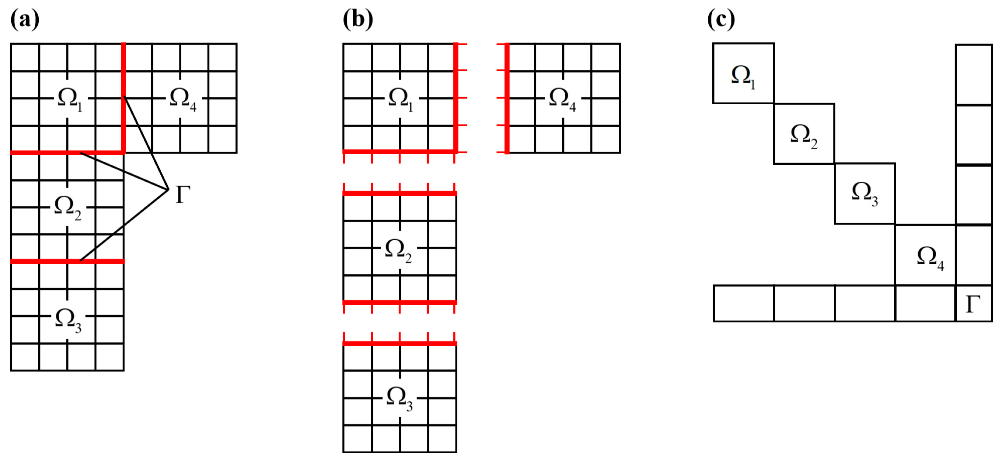
In the Craig–Bampton (CB) method, the entire structure is divided into $n$ substructures that are interconnected at fixed interface boundary $\Gamma$ (Figure 1a). The linear dynamic equations are given by

$$M_g{\ddot{u}}_g+K_g{u}_g=f_g$$

(1a)

$$\mathrm{with} M_g=\left[\begin{array}{cc}{M}_s& M_c\\ M_c^{\mathrm{T}}& M_b\end{array}\right], K_g=\left[\begin{array}{cc}{K}_s& K_c\\ K_c^{\mathrm{T}}& K_b\end{array}\right], u_g=\left[\begin{array}{c}{u}_s\\ u_b\end{array}\right], f_g=\left[\begin{array}{c}{f}_s\\ f_b\end{array}\right],$$

(1b)

$$M_s=\left[\begin{array}{ccc}{M}_s^{(1)}& & 0\\ & \ddots & \\ 0& & M_s^{(n)}\end{array}\right], K_s=\left[\begin{array}{ccc}{K}_s^{(1)}& & 0\\ & \ddots & \\ 0& & K_s^{(n)}\end{array}\right],$$

(1c)

where $K_g$ and $M_g$ represent the global stiffness and mass matrices, respectively, $u_g$ and $f_g$ are the global displacement and force vectors, respectively, and ${(}^{\hspace{0.17em}·\hspace{0.17em}\hspace{0.17em}·})=d^2(\hspace{0.17em}\hspace{0.17em})/d{t}^2$ with the time variable $t$. The subscript $s$, $b$, and $c$ indicate substructure, interface boundary, and coupled terms, respectively. It should be noted that $K_s$ and $M_s$ are block-diagonal stiffness and mass matrices, respectively. These matrices are composed of substructural stiffness and mass matrices, $K_s^{(i)}$ and $M_s^{(i)}$ (for $i=1,\cdots ,n$).

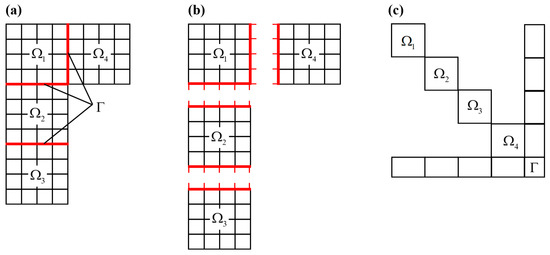
Figure 1. Substructuring the global structure: (a) Global structure with substructures ${\Omega }_i$ (for $i=1,\hspace{0.17em}\hspace{0.17em}2,\hspace{0.17em}\hspace{0.17em}3,\hspace{0.17em}\hspace{0.17em}4$) and interface boundary $\Gamma$; (b) substructures with fixed interface boundary; (c) algebraic representation in the global matrix.

Substructures in the CMS framework can be divided using physical domain-based substructuring, which relies on geometric or topological considerations. Alternatively, algebraic substructuring, as applied in the ECB method discussed in the next section, can also be employed. Algebraic substructuring typically utilizes graph-partitioning algorithms, such as METIS [17], which by default aim to evenly distribute nodes across substructures to balance computational loads.

From Equation (1), the generalized eigenvalue problem for the global structure is obtained as

$$K_g{({\mathit{\varphi }}_g)}_i={\lambda }_i{M}_g{({\mathit{\varphi }}_g)}_i \mathrm{with} i=1,\hspace{0.17em}\hspace{0.17em}2,\hspace{0.17em}\hspace{0.17em}\dots \hspace{0.17em}\hspace{0.17em},\hspace{0.17em}{N}_g,$$

(2)

in which ${({\mathit{\varphi }}_g)}_i$ and ${\lambda }_i$ are the eigenvector and eigenvalue calculated in the global structure, respectively, and $N_g$ is the number of DOFs in the global FE model.

Using the eigenvector calculated in Equation (2), the global displacement vector $u_g$ can be expressed by

$$u_g={\Phi }_g{q}_g$$

(3a)

$$\mathrm{with} {\Phi }_g=\left[\begin{array}{cccc}{({\mathit{\varphi }}_g)}_1& {({\mathit{\varphi }}_g)}_2& \cdots & {({\mathit{\varphi }}_g)}_i\end{array}\right], q_g^{\mathrm{T}}=\left[\begin{array}{cccc}{q}_1& q_2& \cdots & q_i\end{array}\right] \mathrm{for} i=1,2,\cdots ,N_g,$$

(3b)

in which ${\Phi }_g$ represents the global eigenvector matrix, which includes the eigenvectors ${({\mathit{\varphi }}_g)}_i$, while $q_g$ is the generalized coordinate vector comprising the generalized coordinate $q_i$ associated with ${({\mathit{\varphi }}_g)}_i$.

Then, the transformation matrix $T_0$ is constructed as

$$T_0=\left[\begin{array}{cc}{\Phi }_s& {\Psi }_c\\ 0& I_b\end{array}\right]\mathrm{with} {\Phi }_s=\left[\begin{array}{cc}{\Phi }_s^d& {\Phi }_s^r\end{array}\right], {\Psi }_c=-K_s^{-1}{K}_c,$$

(4)

where ${\Phi }_s$ represents the substructural eigenvector matrix, encompassing all substructures. ${\Phi }_s$ consists of the dominant modes matrix ${\Phi }_s^d$ and the residual modes matrix ${\Phi }_s^r$. ${\Psi }_c$ denotes the constraint mode matrix and $I_b$ represents the identity matrix for the interface boundary.

In Equation (4), ${\Phi }_s$ is a block-diagonal eigenvector matrix, with each block corresponding to the substructural eigenvector matrix ${\Phi }_s^{(i)}$ for $i=1,\hspace{0.17em}\hspace{0.17em}2,\hspace{0.17em}\hspace{0.17em}\dots \hspace{0.17em}\hspace{0.17em},\hspace{0.17em}\hspace{0.17em}n$. ${\Phi }_s^{(i)}$ is calculated by solving the following substructural eigenvalue problems

$$K_s^{(i)}{\Phi }_s^{(i)}=M_s^{(i)}{\Phi }_s^{(i)}{\Lambda }_s^{(i)}$$

(5a)

$$\mathrm{with} {\Phi }_s^{(i)}=\left[\begin{array}{cc}{\Phi }_d^{(i)}& {\Phi }_r^{(i)}\end{array}\right], {\Lambda }_s^{(i)}=\left[\begin{array}{cc}{\Lambda }_d^{(i)}& 0\\ 0& {\Lambda }_r^{(i)}\end{array}\right] \mathrm{for} i=1,\hspace{0.17em}\hspace{0.17em}2,\hspace{0.17em}\hspace{0.17em}\dots \hspace{0.17em}\hspace{0.17em},\hspace{0.17em}\hspace{0.17em}n,$$

(5b)

where ${\Lambda }_s^{(i)}$ is the substructural eigenvalue matrix for the $i^{\mathrm{th}}$ substructure, and ${\Phi }_s^{(i)}$ and ${\Lambda }_s^{(i)}$ are each composed of a dominant term (${\Phi }_d^{(i)}$, ${\Lambda }_d^{(i)}$) and a residual term (${\Phi }_r^{(i)}$, ${\Lambda }_r^{(i)}$).

The constraint mode matrix ${\Psi }_c$ in Equation (4) is calculated as follows:

$${\Psi }_c=\left[\begin{array}{c}{\Psi }_c^{(1)}\\ ⋮\\ {\Psi }_c^{(n)}\end{array}\right]\mathrm{with} {\Psi }_c^{(i)}=-{(K_s^{(i)})}^{-1}{K}_c^{(i)}\mathrm{for} i=1,\hspace{0.17em}\hspace{0.17em}2,\hspace{0.17em}\hspace{0.17em}\dots \hspace{0.17em}\hspace{0.17em},\hspace{0.17em}\hspace{0.17em}n,$$

(6)

in which ${\Psi }_c^{(i)}$ represents the constraint mode matrix for the $i^{\mathrm{th}}$ substructure.

The global displacement vector $u_g$ is converted using the transformation matrix $T_0$ in Equation (4), as follows:

$$u_g=\left[\begin{array}{c}{u}_s\\ u_b\end{array}\right]=T_{0}u\mathrm{with} T_0=\left[\begin{array}{ccc}{\Phi }_s^d& {\Phi }_s^r& {\Psi }_c\\ 0& 0& I_b\end{array}\right], u=\left[\begin{array}{c}{q}_s^d\\ q_s^r\\ u_b\end{array}\right],$$

(7)

where $u$ represents the generalized coordinate vector, and its components $q_s^d$ and $q_s^r$ are the modal coordinate vectors corresponding to ${\Phi }_s^d$ and ${\Phi }_s^r$, respectively.

In Equation (7), the approximated global displacement vector ${\overline{u}}_g$ is obtained by retaining only the dominant terms ${\Phi }_s^d$ and $q_s^d$, as follows:

$$u_g\approx {\overline{u}}_g={\overline{T}}_{\mathrm{CB}}{\overline{u}}_{\mathrm{CB}}\mathrm{with} {\overline{T}}_{\mathrm{CB}}=\left[\begin{array}{cc}{\Phi }_s^d& {\Psi }_c\\ 0& I_b\end{array}\right], {\overline{u}}_{\mathrm{CB}}=\left[\begin{array}{c}{q}_s^d\\ u_b\end{array}\right],$$

(8)

in which ${\overline{T}}_{\mathrm{CB}}$ represents the reduced transformation matrix in the CB method, and ${\overline{u}}_{\mathrm{CB}}$ is the corresponding generalized coordinate vector. In this notation, ${(}^{\hspace{0.17em}-})$ indicates the approximated quantities.

Using ${\overline{T}}_{\mathrm{CB}}$ in Equation (8), the reduced equations of motion for the partitioned structure are expressed as

$${\overline{M}}_{\mathrm{CB}}{\ddot{\overline{u}}}_{\mathrm{CB}}+{\overline{K}}_{\mathrm{CB}}{\overline{u}}_{\mathrm{CB}}={\overline{f}}_{\mathrm{CB}}$$

(9a)

with

$${\overline{M}}_{\mathrm{CB}}={\overline{T}}_{\mathrm{CB}}^{\mathrm{T}}{M}_g{\overline{T}}_{\mathrm{CB}}=\left[\begin{array}{cc}{I}_s^d& {({\Phi }_s^d)}^{\mathrm{T}}{\widehat{M}}_c\\ {\widehat{M}}_c^{\mathrm{T}}({\Phi }_s^d)& {\widehat{M}}_b\end{array}\right],$$

(9b)

$${\overline{K}}_{\mathrm{CB}}={\overline{T}}_{\mathrm{CB}}^{\mathrm{T}}{K}_g{\overline{T}}_{\mathrm{CB}}=\left[\begin{array}{cc}{\Lambda }_s^d& 0\\ 0& {\widehat{K}}_b\end{array}\right], {\overline{f}}_{\mathrm{CB}}={\overline{T}}_{\mathrm{CB}}^{\mathrm{T}}\left[\begin{array}{c}{f}_s\\ f_b\end{array}\right],$$

(9c)

where

$$I_s^d={({\Phi }_s^d)}^{\mathrm{T}}{M}_s({\Phi }_s^d), {\widehat{M}}_c=M_c+M_s{\Psi }_c, {\widehat{M}}_b=M_b+M_c^{\mathrm{T}}{\Psi }_c+{\Psi }_c^{\mathrm{T}}{\widehat{M}}_c,$$

(9d)

$${\Lambda }_s^d={({\Phi }_s^d)}^{\mathrm{T}}{K}_s({\Phi }_s^d), {\widehat{K}}_b=K_b+K_c^{\mathrm{T}}{\Psi }_c,$$

(9e)

in which ${\overline{M}}_{\mathrm{CB}}$ and ${\overline{K}}_{\mathrm{CB}}$ represent the reduced matrices with sizes of ${\overline{N}}_{\mathrm{CB}}\times {\overline{N}}_{\mathrm{CB}}$ (${\overline{N}}_{\mathrm{CB}}={\overline{N}}_s^d+N_b$, where ${\overline{N}}_s^d$ and $N_b$ are the numbers of dominant substructural modes and interface boundary DOFs, respectively), and ${\overline{u}}_{\mathrm{CB}}$ and ${\overline{f}}_{\mathrm{CB}}$ are the approximated displacement and force vectors, respectively.

From Equation (9), the reduced eigenvalue problem is formulated as

$${\overline{K}}_{\hspace{0.17em}\hspace{0.17em}\mathrm{CB}}{({\overline{\mathit{\varphi }}}_{\hspace{0.17em}\hspace{0.17em}\mathrm{CB}})}_i={\overline{\lambda }}_{\hspace{0.17em}\mathrm{CB},i}{\overline{M}}_{\hspace{0.17em}\hspace{0.17em}\mathrm{CB}}{({\overline{\mathit{\varphi }}}_{\hspace{0.17em}\hspace{0.17em}\mathrm{CB}})}_i \mathrm{for} i=1,\hspace{0.17em}\hspace{0.17em}2,\hspace{0.17em}\hspace{0.17em}\dots \hspace{0.17em}\hspace{0.17em},\hspace{0.17em}\hspace{0.17em}{\overline{N}}_{\mathrm{CB}},$$

(10)

in which ${\overline{\lambda }}_{\mathrm{CB},i}$ and ${({\overline{\mathit{\varphi }}}_{\hspace{0.17em}\hspace{0.17em}\mathrm{CB}})}_i$ are the eigenvalue and eigenvector calculated in the reduced order model, respectively.

With the eigenvectors obtained from Equation (10), the approximated displacement vector ${\overline{u}}_{\mathrm{CB}}$ in Equation (8) is represented by

$${\overline{u}}_{\mathrm{CB}}={\overline{\Phi }}_{\mathrm{CB}}{\overline{\lambda }}_{\mathrm{CB}}\mathrm{with} {\overline{\Phi }}_{\mathrm{CB}}=\left[\begin{array}{ccc}{({\overline{\mathit{\varphi }}}_{\hspace{0.17em}\hspace{0.17em}\mathrm{CB}})}_1& \cdots & {({\overline{\mathit{\varphi }}}_{\hspace{0.17em}\hspace{0.17em}\mathrm{CB}})}_{{\overline{N}}_{\mathrm{CB}}}\end{array}\right],$$

(11)

where ${\overline{\Phi }}_{\mathrm{CB}}$ is the eigenvector matrix in the reduced model and ${\overline{\lambda }}_{\mathrm{CB}}$ is the corresponding generalized coordinate vector.

2.2. ECB Method

In the CB method, only the dominant normal modes of the substructures are retained, which can result in a loss of accuracy. The recently developed ECB method enhances efficiency by utilizing algebraic partitioning, allowing for the creation of a larger number of substructures [15,17,18,23,24,25]; see Figure 1c. Furthermore, this method significantly improves accuracy by considering the effects of residual normal modes through the use of residual flexibility matrices for each substructure.

Additionally, in the CB method, the number of interface boundary DOFs increases as the number of substructures grows. The ECB method addresses this by performing interface boundary DOF reduction, ensuring computational efficiency is maintained.

The eigenvalue problem for the interface boundary with the mass and stiffness matrices for the interface boundary, ${\widehat{M}}_b$ and ${\widehat{K}}_b$, in Equation (9) is given as follows:

$${\widehat{K}}_b{\Phi }_b={\widehat{M}}_b{\Phi }_b{\Lambda }_b\mathrm{with} {\Phi }_b=\left[\begin{array}{cc}{\Phi }_b^d& {\Phi }_b^r\end{array}\right], {\Lambda }_b=\left[\begin{array}{cc}{\Lambda }_b^d& 0\\ 0& {\Lambda }_b^r\end{array}\right],$$

(12)

where ${\Phi }_b^d$ and ${\Phi }_b^r$ are the eigenvector and eigenvalue matrices for the interface boundary, and those are divided into dominant terms (${\Phi }_b^d$ and ${\Lambda }_b^d$) and residual terms (${\Phi }_b^r$ and ${\Lambda }_b^r$).

Using eigenvector and eigenvalue matrices in Equation (12), the interface displacement vector $u_b$ in Equation (7) can be represented as follows:

$$u_b={\Phi }_b{q}_b=\left[\begin{array}{cc}{\Phi }_b^d& {\Phi }_b^r\end{array}\right]\left[\begin{array}{c}{q}_b^d\\ q_b^r\end{array}\right],$$

(13)

in which $q_b$ is the modal coordinate vector associated with ${\Phi }_b$, and it is decomposed into dominant and residual terms, $q_b^d$ and $q_b^r$.

Using Equation (13), the global displacement vector $u_g$ in Equation (7) is rewritten as

$$u_g=T_{0}u=T_0\left(T_{b}q\right)=Tq$$

(14a)

$$\mathrm{with} T_b=\left[\begin{array}{cccc}{I}_s^d& 0& 0& 0\\ 0& I_s^d& 0& 0\\ 0& 0& {\Phi }_b^d& {\Phi }_b^r\end{array}\right], q=\left[\begin{array}{c}{q}_s^d\\ q_s^r\\ q_b^d\\ q_b^r\end{array}\right], T=T_0{T}_b=\left[\begin{array}{cccc}{\Phi }_s^d& {\Phi }_s^r& {\Psi }_c{\Phi }_b^d& {\Psi }_c{\Phi }_b^r\\ 0& 0& {\Phi }_b^d& {\Phi }_b^r\end{array}\right],$$

(14b)

where $T_b$ is the interface transformation matrix, $T$ is the transformation matrix composed of the eigenmodes of the substructure and interface boundary, and $q$ is the modal coordinate vector associated with the transformation matrix $T$.

After reordering the columns of the $T$ matrix based on the dominant and residual terms, the global displacement vector $u_g$ is reformulated as follows:

$$u_g=Tq=\left[\begin{array}{cc}{T}_d& T_r\end{array}\right]\left[\begin{array}{c}{q}_d\\ q_r\end{array}\right]$$

(15a)

$$\mathrm{with} T_d=\left[\begin{array}{cc}{\Phi }_s^d& {\Psi }_c{\Phi }_b^d\\ 0& {\Phi }_b^d\end{array}\right], T_r=\left[\begin{array}{cc}{\Phi }_s^r& {\Psi }_c{\Phi }_b^r\\ 0& {\Phi }_b^r\end{array}\right], q_d=\left[\begin{array}{c}{q}_s^d\\ q_b^d\end{array}\right], q_r=\left[\begin{array}{c}{q}_s^r\\ q_b^r\end{array}\right],$$

(15b)

where $T_d$ and $T_r$ are the dominant and residual parts of the transformation matrix $T$, and $q_d$ and $q_r$ are the modal coordinate vectors associated with $T_d$ and $T_r$, respectively.

Focusing only the dominant part $T_d$ in Equation (15b), the global displacement vector $u_g$ could be approximated as follows:

$$u_g\approx {\tilde{u}}_g={\tilde{T}}_d{\tilde{q}}_d\mathrm{with} {\tilde{T}}_d=T_d, {\tilde{q}}_d=q_d.$$

(16)

In this notation, (^~) indicates the approximated quantities.

With the approximation in Equation (16), the reduced eigenvalue problem can be expressed as

$$\tilde{K}{\tilde{q}}_d=\tilde{\lambda }\tilde{M}{\tilde{q}}_d$$

(17a)

with

$$\tilde{M}={\tilde{T}}_d^{\mathrm{T}}{M}_g{\tilde{T}}_d=\left[\begin{array}{cc}{I}_s^d& {\tilde{M}}_c\\ {\tilde{M}}_c^{\mathrm{T}}& I_b^d\end{array}\right], \tilde{K}={\tilde{T}}_d^{\mathrm{T}}{K}_g{\tilde{T}}_d=\left[\begin{array}{cc}{\Lambda }_s^d& 0\\ 0& {\Lambda }_b^d\end{array}\right],$$

(17b)

$$I_s^d={({\Phi }_b^d)}^{\mathrm{T}}{\widehat{M}}_b({\Phi }_b^d), {\tilde{M}}_c={({\Phi }_s^d)}^{\mathrm{T}}{\widehat{M}}_c({\Phi }_s^d), {\Lambda }_b^d={({\Phi }_b^d)}^{\mathrm{T}}{\widehat{K}}_b({\Phi }_b^d),$$

(17c)

in which $\tilde{M}$ and $\tilde{K}$ are the reduced mass and stiffness matrices accounting for the substructure and the interface reduction [25], and $\tilde{\lambda }$ is the approximated eigenvalue.

In the ECB method, the residual substructural mode is compensated in the transformation matrix ${\tilde{T}}_d$ containing dominant modes of substructures and interface boundary.

The transformation matrix of the ECB method is enhanced to

$${\tilde{T}}_{\mathrm{ECB}}={\tilde{T}}_d+T_{a}R$$

(18a)

$$\mathrm{with} T_a=\left[\begin{array}{cc}0& F_s^{rs}{\widehat{M}}_c{\Phi }_b^d\\ 0& 0\end{array}\right], R={\tilde{M}}^{-1}\tilde{K},$$

(18b)

where ${\tilde{T}}_d$ is the dominant part of the transformation matrix $T$ in Equation (14), $\tilde{M}$ and $\tilde{K}$ are the reduced mass and stiffness matrices in the CB method accounting for the interface reduction [24] in Equation (17b), and ${\widehat{M}}_c$ is the submatrix of the CB method in Equation (9d). $F_s^{rs}$ is the static residual flexibility matrix for substructures, defined by

$$\begin{gathered} F_s^{rs}=\left[\begin{array}{ccc}{F}_s^{(1)}& & 0\\ & \ddots & \\ 0& & F_s^{(n)}\end{array}\right]\mathrm{with} F_s^{(i)}={(K_s^{(i)})}^{-1}-({\Phi }_d^{(i)}){({\Lambda }_d^{(i)})}^{-1}{({\Phi }_d^{(i)})}^{\mathrm{T}} \\ \mathrm{for} i=1,\hspace{0.17em}\hspace{0.17em}2,\hspace{0.17em}\hspace{0.17em}\dots \hspace{0.17em}\hspace{0.17em},\hspace{0.17em}\hspace{0.17em}n. \end{gathered}$$

(19)

The residual substructural eigenvector matrix ${\Phi }_s^r$ in Equation (7) is reflected into the transformation matrix of the ECB method ${\tilde{T}}_{\mathrm{ECB}}$ through the static residual flexibility matrix $F_s^{rs}$ in Equation (19).

The global displacement vector $u_g$ is approximated by using the transformation matrix ${\tilde{T}}_{\mathrm{ECB}}$ described in Equation (18) as follows:

$$u_g\approx {\tilde{u}}_g={\tilde{T}}_{\mathrm{ECB}}{\tilde{q}}_{\mathrm{ECB}},$$

(20)

where ${\tilde{q}}_{\mathrm{ECB}}$ is the dominant modal coordinate vector approximated by applying the ECB method.

Substituting Equation (20) into the linear dynamic equation in Equation (1), the reduced equations of motion is given by

$${\tilde{M}}_{\mathrm{ECB}}{\ddot{\tilde{q}}}_{\mathrm{ECB}}+{\tilde{K}}_{\mathrm{ECB}}{\tilde{q}}_{\mathrm{ECB}}={\tilde{f}}_{\mathrm{ECB}},$$

(21a)

with

$${\tilde{M}}_{\mathrm{ECB}}={\tilde{T}}_{\mathrm{ECB}}^{\mathrm{T}}{M}_g{\tilde{T}}_{\mathrm{ECB}}=\tilde{M}+Y, {\tilde{K}}_{\mathrm{ECB}}={\tilde{T}}_{\mathrm{ECB}}^{\mathrm{T}}{K}_g{\tilde{T}}_{\mathrm{ECB}}=\tilde{K},$$

(21b)

$$Y=T_d^{\mathrm{T}}{M}_g{T}_{a}R, {\tilde{f}}_{\mathrm{ECB}}={\tilde{T}}_{\mathrm{ECB}}^{\mathrm{T}}\left[\begin{array}{c}{f}_s\\ f_b\end{array}\right],$$

(21c)

in which ${\tilde{M}}_{\mathrm{ECB}}$ and ${\tilde{K}}_{\mathrm{ECB}}$ are reduced matrices of size ${\overline{N}}_{\mathrm{ECB}}\times {\overline{N}}_{\mathrm{ECB}}$ with ${\overline{N}}_{\mathrm{ECB}}={\overline{N}}_s^d+{\overline{N}}_b^d$, and ${\overline{N}}_b^d$ denotes the number of dominant interface boundary modes selected.

Based on Equation (21a), the reduced eigenvalue problem is given by

$${\tilde{K}}_{\hspace{0.17em}\hspace{0.17em}\mathrm{ECB}}{({\tilde{\mathit{\varphi }}}_{\hspace{0.17em}\hspace{0.17em}\mathrm{ECB}})}_i={\tilde{\lambda }}_{\hspace{0.17em}\mathrm{ECB},i}{\tilde{M}}_{\hspace{0.17em}\hspace{0.17em}\mathrm{ECB}}{({\tilde{\mathit{\varphi }}}_{\hspace{0.17em}\hspace{0.17em}\mathrm{ECB}})}_i \mathrm{for} i=1,\hspace{0.17em}\hspace{0.17em}2,\hspace{0.17em}\hspace{0.17em}\dots \hspace{0.17em}\hspace{0.17em},\hspace{0.17em}\hspace{0.17em}{\overline{N}}_{\mathrm{ECB}},$$

(22)

where ${\tilde{\lambda }}_{\mathrm{ECB},i}$ and ${({\tilde{\mathit{\varphi }}}_{\hspace{0.17em}\hspace{0.17em}\mathrm{ECB}})}_i$ are the eigenvalue and eigenvector calculated in the reduced model, respectively.

Using the eigenvectors obtained from Equation (22), the approximated dominant modal coordinate vector ${\tilde{q}}_{\mathrm{ECB}}$ corresponding to the transformation matrix of the ECB method ${\tilde{T}}_{\mathrm{ECB}}$ in Equation (18a) is given by

$${\tilde{q}}_{\mathrm{ECB}}={\tilde{\Phi }}_{\mathrm{ECB}}{\tilde{\lambda }}_{\mathrm{ECB}}\mathrm{with} {\tilde{\Phi }}_{\mathrm{ECB}}=\left[\begin{array}{ccc}{({\tilde{\mathit{\varphi }}}_{\hspace{0.17em}\hspace{0.17em}\mathrm{ECB}})}_1& \cdots & {({\tilde{\mathit{\varphi }}}_{\hspace{0.17em}\hspace{0.17em}\mathrm{ECB}})}_{{\overline{N}}_{\mathrm{ECB}}}\end{array}\right],$$

(23)

in which ${\tilde{\Phi }}_{\mathrm{ECB}}$ is the eigenvector matrix calculated based on the reduced eigenvalue problem in Equation (22) and ${\tilde{\lambda }}_{\mathrm{ECB}}$ is the corresponding generalized coordinate vector.

The automatic matrix partitioning strategy, algorithms, and detailed mathematical formulations used in this method can be found in [14].

3. Direct Time-Response Analysis Using the Reduced Order Model

In this section, we present a strategy for performing time history response analysis by applying the ECB method to create a reduced order model. This approach focuses on improving computational efficiency by applying the transformation matrix selectively to regions of interest rather than to the entire domain, aligning with scenarios where responses are required only for specific local areas.

3.1. Time Integration Using the Newmark Method

To obtain the time history response of the reduced linear dynamic equations in Equation (21), we employ the average acceleration Newmark time integration method, a widely used time integration technique for dynamic analysis. The equations for time integrations are given as follows:

$${\dot{\tilde{q}}}_{\mathrm{ECB}}(t+\Delta t)={\dot{\tilde{q}}}_{\mathrm{ECB}}(t)+0.5\left\{{\ddot{\tilde{q}}}_{\mathrm{ECB}}(t)+{\ddot{\tilde{q}}}_{\mathrm{ECB}}(t+\Delta t)\right\}\Delta t,$$

(24a)

$${\tilde{q}}_{\mathrm{ECB}}(t+\Delta t)={\tilde{q}}_{\mathrm{ECB}}(t)+{\dot{\tilde{q}}}_{\mathrm{ECB}}(t)\Delta t+0.25\left\{{\ddot{\tilde{q}}}_{\mathrm{ECB}}(t)+{\ddot{\tilde{q}}}_{\mathrm{ECB}}(t+\Delta t)\right\}\Delta t^2,$$

(24b)

where $\Delta t$ denotes the time step. Through these equations, the displacement, velocity, and acceleration vectors of the reduced order model are calculated over time.

3.2. Back-Transformation Process to Compute the Global Displacement

After the time integration of the reduced order model, the full response of the original finite element model can be reconstructed through a back-transformation calculation. This process involves transforming the reduced order model responses back to the full set of degrees of freedom:

$${\tilde{u}}_g={\tilde{T}}_{\mathrm{ECB}}{\tilde{q}}_{\mathrm{ECB}}, {\dot{\tilde{u}}}_g={\tilde{T}}_{\mathrm{ECB}}{\dot{\tilde{q}}}_{\mathrm{ECB}}, {\ddot{\tilde{u}}}_g={\tilde{T}}_{\mathrm{ECB}}{\ddot{\tilde{q}}}_{\mathrm{ECB}}$$

(25)

in which ${\tilde{T}}_{\mathrm{ECB}}$ is the transformation matrix derived from the ECB method in Equation (18a). Although this full back-transformation process in Equation (25) allows for the recovery of the full model response, the transformation matrix ${\tilde{T}}_{\mathrm{ECB}}$ is generally dense, making this process computationally intensive.

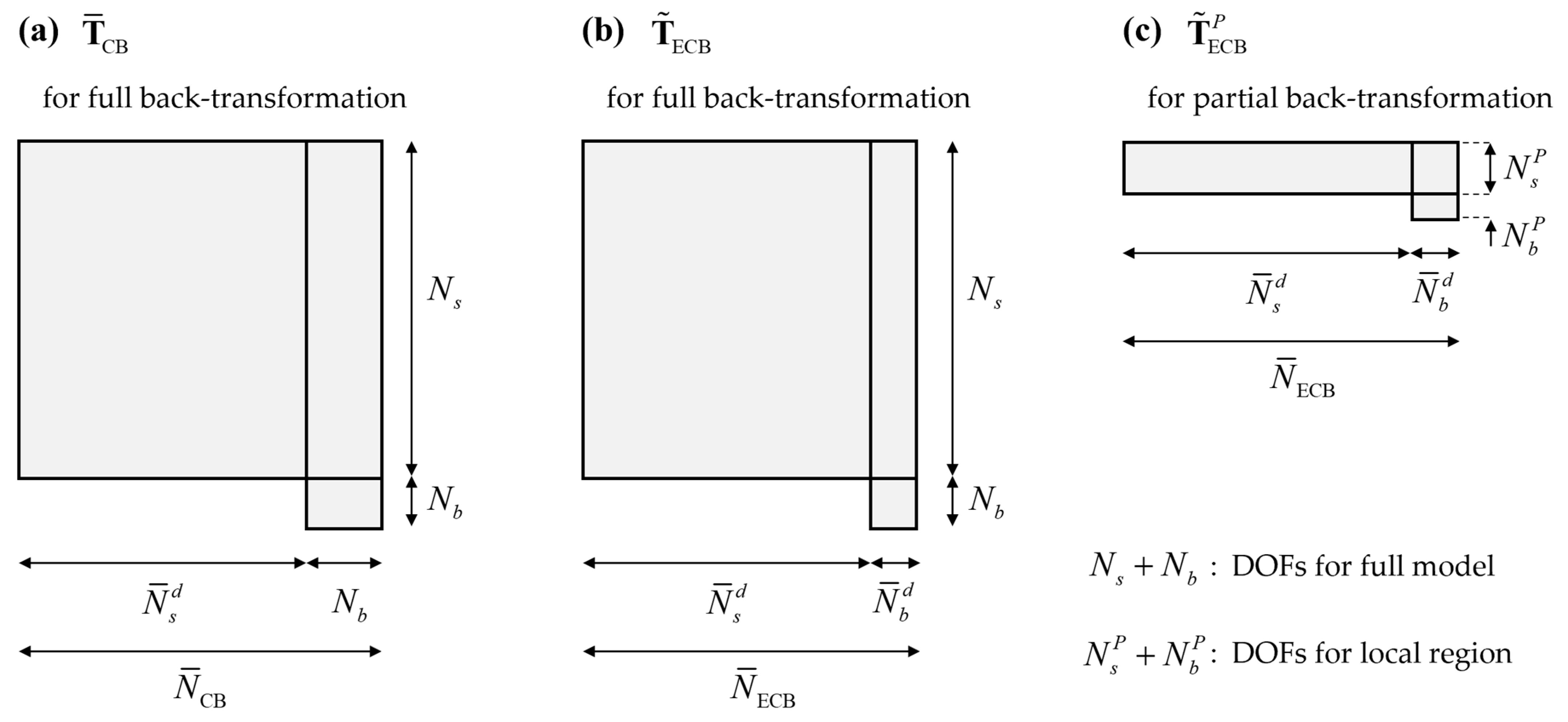
To further improve efficiency, especially when responses are needed only for specific local regions, a partial back-transformation process can be applied. This approach involves a reduced transformation matrix ${\tilde{T}}_{\mathrm{ECB}}^{\mathrm{P}}$, which is constructed to target only the degrees of freedom within regions of interest (see Figure 2). The response for these selected areas is then computed as follows:

$${\tilde{u}}_g^P={\tilde{T}}_{\mathrm{ECB}}^P{\tilde{q}}_{\mathrm{ECB}}, {\dot{\tilde{u}}}_g^P={\tilde{T}}_{\mathrm{ECB}}^P{\dot{\tilde{q}}}_{\mathrm{ECB}}, {\ddot{\tilde{u}}}_g^P={\tilde{T}}_{\mathrm{ECB}}^P{\ddot{\tilde{q}}}_{\mathrm{ECB}}$$

(26)

where ${\tilde{u}}_g^{\mathrm{P}}$, $\hspace{0.17em}{\dot{\tilde{u}}}_g^P$, and $\hspace{0.17em}{\ddot{\tilde{u}}}_g^P$ denote the global displacement, velocity, and acceleration vectors for the chosen regions. While the full back-transformation process in Equation (25) allows for the recovery of the complete model response, it is computationally intensive due to the dense nature of the transformation matrix. In contrast, the partial back-transformation process, as expressed in Equation (26), offers significant computational advantages by focusing only on specific regions of interest. This approach reduces the scope of matrix operations, minimizes memory usage, and decreases computation time, making it particularly efficient for localized response evaluations.

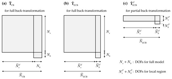
Figure 2. The transformation matrices of (a) the CB method for full back-transformation process, (b) the ECB method for full back-transformation process, and (c) the reduced transformation matrix of the ECB method for partial back-transformation process. Here, $N_s$, $N_b$, $N_s^P$, and $N_b^P$ represent the substructure DOFs, the interface boundary DOFs, the number of selected DOFs in substructures, and the number of selected DOFs in the interface boundary, respectively.

The code utilized in this study is an academic MATLAB code specifically developed by the authors for the analyses conducted in this research. To provide clarity on the computational process, a detailed workflow has been presented in Table 1.

Table 1. Computational procedure of the direct time-response analysis with CB and ECB methods.

Computational Procedure	Related Equations and Figures
Generate FE global matrices and vectors	Equation (1a)
Substructuring	Equation (1b,c), Figure 1
Construct reduced equations of motion
- CB method	Equation (9)
- ECB method	Equation (21)
Time integration	Equation (24)
Partial back-transformation	Equation (26)

4. Numerical Examples

This section evaluates the performance of the ECB method in direct time-response analysis through numerical examples. The results obtained using the ECB method are compared with those from the full finite element model and the CB method. The CB method, as one of the most fundamental and widely used techniques associated with the fixed-interface CMS method, was chosen as a comparative baseline due to its widespread adoption in both academic research and commercial applications. This comparison highlights the computational efficiency and accuracy improvements achieved by the ECB method while ensuring reliable results are achieved for practical engineering applications.

The ECB method used in this study is a fixed-interface CMS technique that has undergone multiple advancements over the years. While the original CB method serves as the foundational approach, the ECB method has been continuously refined to address its limitations. As the model size increases, achieving accurate results with reduced models requires significantly more substructuring. In this context, the ECB method demonstrates its effectiveness over the CB method by achieving higher accuracy and computational efficiency. Previous studies, as referenced in [14], provide detailed comparisons between earlier versions of the ECB method and the latest advancements applied in this paper, particularly in terms of accuracy and efficiency for eigenvalue analysis. In this study, the primary focus is to evaluate the performance of the novel ECB method in terms of accuracy and efficiency for direct time-response analysis using reduced order models.

Three benchmark examples, including a cantilever plate, an insulation panel, and a robot arm, are used to assess the ECB method. The accuracy of the reduced models is validated by examining the relative eigenvalue errors and the displacement time history. We also compare the computation times of the full model, CB, and ECB methods to evaluate their efficiency. Simulations are conducted in MATLAB 2021b on a system with an Intel i9-11900KF 3.50 GHz CPU and 64 GB of RAM. The Newmark method is employed for the analysis, with the parameters set to $\beta =0.25$ and $\gamma =0.5$.

The reduced order models are constructed by varying the number of substructures, the number of dominant substructural modes, and the interface boundary DOFs. Particular attention is given to the selection of dominant substructural modes for each substructure. Using METIS 5.1.0 for algebraic substructuring, the number of nodes counts across substructures are made approximately uniform, leading to a consistent number of dominant substructural modes being retained for all substructures. While reducing the number of dominant substructural modes decreases the size of the reduced order model, it can negatively affect the accuracy of global mode representation. A convergence study included in the cantilever plate example highlights the trade-offs between model size and accuracy, emphasizing the importance of selecting an appropriate number of dominant substructural modes when constructing reduced order models using the CB and ECB methods.

4.1. Cantilever Plate

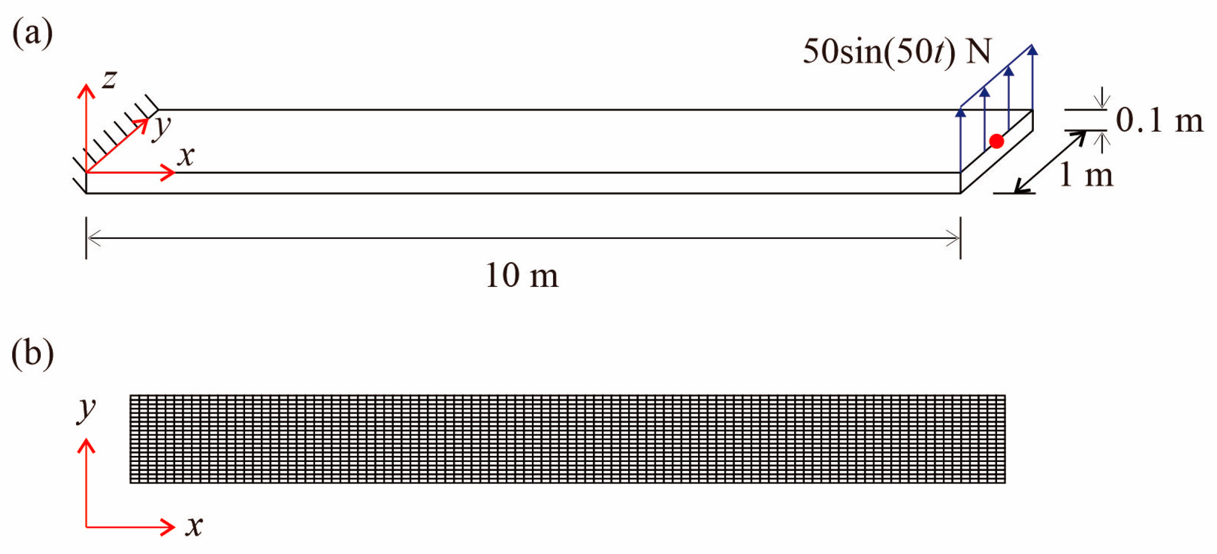
The first example is a cantilever plate subjected to a harmonic loading, as illustrated in Figure 3a. The plate dimensions are a length of 10 m, width of 1 m, and thickness of 0.1 m. The material properties are defined by an elastic modulus of $2.1\times {10}^{11}\hspace{0.17em}\hspace{0.17em}{\mathrm{N}/\mathrm{m}}^2$, a Poisson’s ratio of 0.3, and a density of $7850\hspace{0.17em}\hspace{0.17em}{\mathrm{kg}/\mathrm{m}}^3$. One end of the cantilever plate is fixed, while a harmonic load with a total magnitude of $50\hspace{0.17em}\hspace{0.17em}\mathrm{N}$ and an angular frequency of 50 rad/s is uniformly distributed along the free end in the $z$-direction. The finite element model consists of a 100 $\times$ 20 mesh of the four-node MITC4 shell elements with 10,500 free DOFs, as illustrated in Figure 3b [26,27,28].

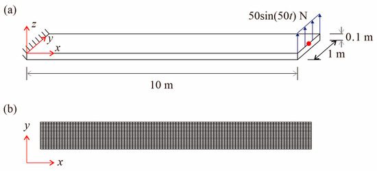
Figure 3. Cantilever plate problem: (a) problem description; (b) a 100 $\times$ 20 mesh of 4-node shell elements with 10,500 free DOFs.

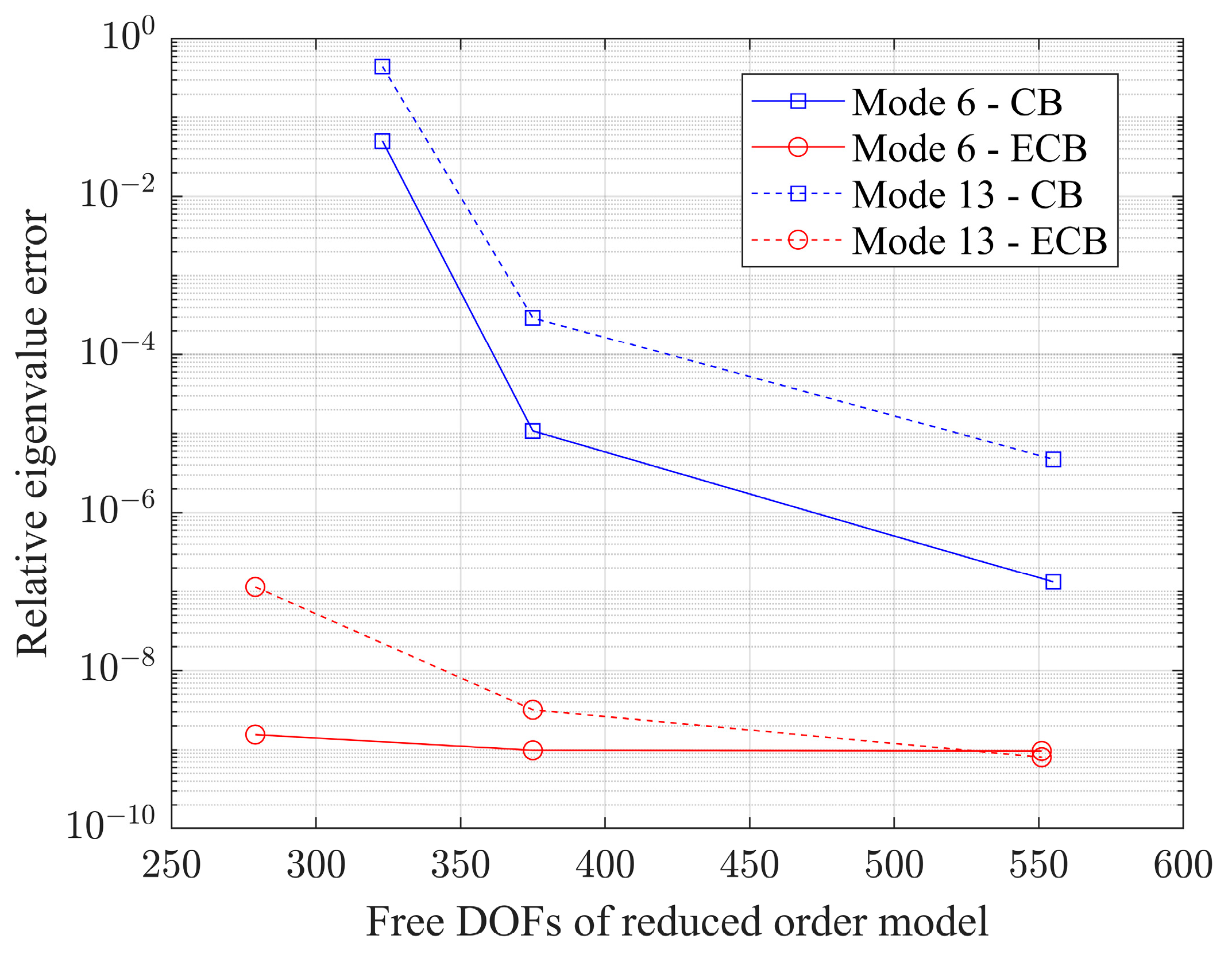
Before conducting a dynamic analysis, we investigate the convergence behavior of the CB and ECB methods by varying the configuration of the reduced order model. For the CB method, the number of substructures is fixed at four, and the number of dominant substructural normal modes is set to 2, 15, and 60, resulting in free DOFs of 323, 375, and 555. Similarly, for the ECB method, the number of substructures is fixed at 16, with 5, 11, and 22 dominant modes, corresponding to free DOFs of 279, 375, and 551, respectively. The interface boundary DOFs are 315 for the CB method and 199 for the ECB method. Figure 4 presents the convergence curves of relative eigenvalue errors for the 6th and 13th modes, illustrating improved accuracy with an increasing number of dominant substructural modes. These results underscore the trade-offs between model size reduction and accuracy, highlighting the importance of selecting proper parameters in the CB and ECB methods.

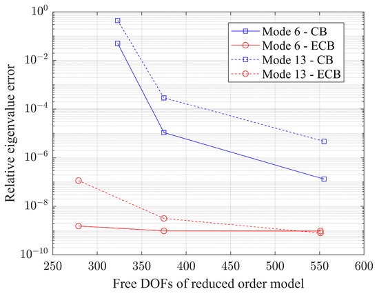
Figure 4. Relative eigenvalue errors for the 6th and 13th modes of the CB and ECB reduced order models with respect to the number of dominant substructural normal modes.

Next, the direct response analysis is conducted over a total time of 5 s with a time step of 0.001 s. After time integration of the reduced model, the full response is reconstructed through back-transformation. In this example, the region of interest for partial back-transformation is defined as the DOFs at the load application region.

Table 2 provides detailed information on the CB and ECB reduced order models. In this direct response analysis, both the CB and ECB models are configured to have the same reduced DOFs of 375, accounting for approximately 3.57% of the 10,500 free DOFs of the full model.

Table 2. Specifications of the CB and ECB reduced order models for the cantilever plate problem. The full model has a total of 10,500 free DOFs.

	CB	ECB
Number of substructures	4	16
Number of dominant substructural normal modes	60 (=4 $\times$ 15)	176 (=16 $\times$ 11)
Interface boundary DOFs	315	-
Reduced interface boundary DOFs	-	199
Total reduced DOFs	375	375

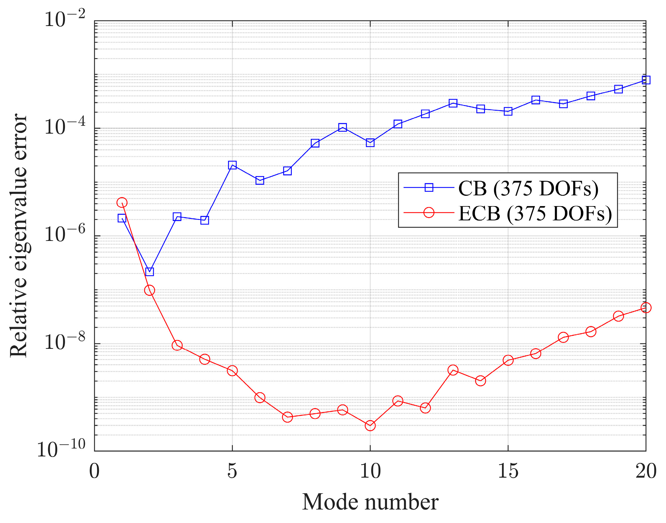
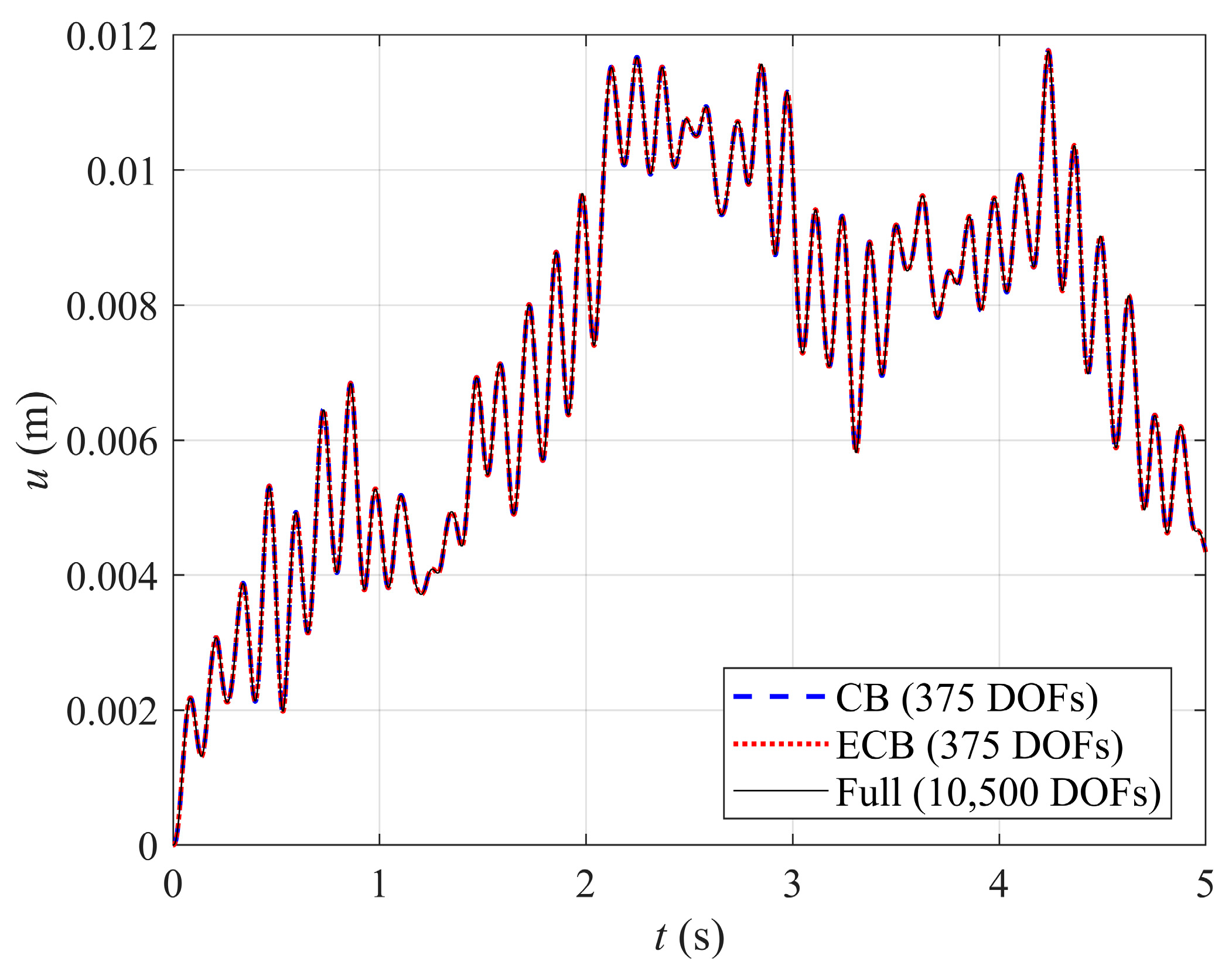
Figure 5 shows the relative eigenvalue errors for modes 1 to 20 for the CB and ECB reduced order models, with the full model results used as the reference. The ECB reduced model provides more accurate results than the CB reduced order model. Figure 6 presents the time history of $z$-direction displacement at the red-marked point. Despite the significantly reduced DOFs, both reduced models provide displacement results that are nearly identical to those of the full model. Table 3 presents the solution times for direct time-response analysis. This example confirms that the reduction methods, CB and ECB, work effectively in direct time-response analysis. In the following example, a larger-scale problem is considered to allow for a more detailed comparison between CB and ECB methods.

Figure 5. Relative eigenvalue errors of modes 1 to 20 for the cantilever plate problem.

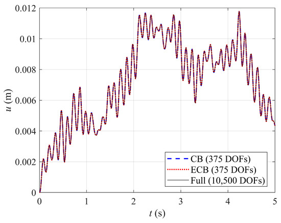
Figure 6. Displacement time history at the red-marked point for the cantilever plate problem.

Table 3. Solution times of direct time-response analyses for the cantilever plate problem (in seconds).

	Full Model	CB	ECB
Reduction	-	0.74	1.28
Newmark	7.41	0.65	0.77
Partial back-transformation	-	0.52	0.51
Total	7.41	1.92	2.57

4.2. Insulation Panel

The second example is an insulation panel subjected to an impact loading, as shown in Figure 7a. This setup represents the evaluation of the structural strength of the cargo containment system in LNG carriers under impact loading caused by sloshing. As shown in Figure 7b, the insulation panel is modeled using two materials: plywood and reinforced polyurethane foam (R-PUF). The elastic modulus, density, and Poisson’s ratio of plywood are 8900 MPa, $710\hspace{0.17em}\hspace{0.17em}{\mathrm{kg}/\mathrm{m}}^3$, and 0.17, respectively, while those of R-PUF are 84 MPa, $120\hspace{0.17em}\hspace{0.17em}{\mathrm{kg}/\mathrm{m}}^3$, and 0.18, respectively. The bottom surface ($z=0\hspace{0.17em}\hspace{0.17em}\mathrm{mm}$) is fixed, while uniformly distributed impact loading is applied to the top surface ($z=300\hspace{0.17em}\hspace{0.17em}\mathrm{mm}$), with its total magnitude (unit: $\mathrm{N}$) defined as follows:

$$f(t)=\left\{\hspace{0.17em}\begin{array}{c}\hspace{0.17em}{\displaystyle \frac{t}{T_{\mathrm{rise}}}}\hspace{0.17em}\hspace{0.17em}\hspace{0.17em}\hspace{0.17em}\hspace{0.17em}\hspace{0.17em}\hspace{0.17em}\hspace{0.17em}\hspace{0.17em}0\le t<T_{\mathrm{rise}}\\ 2-{\displaystyle \frac{t}{T_{\mathrm{rise}}}}\hspace{0.17em}\hspace{0.17em}\hspace{0.17em}\hspace{0.17em}\hspace{0.17em}\hspace{0.17em}\hspace{0.17em}\hspace{0.17em}\hspace{0.17em}{T}_{\mathrm{rise}}\le t\le 2T_{\mathrm{rise}}\end{array}\right.\hspace{0.17em}\hspace{0.17em}\hspace{0.17em}\hspace{0.17em}\hspace{0.17em}\mathrm{with}\hspace{0.17em}\hspace{0.17em}\hspace{0.17em}\hspace{0.17em}\hspace{0.17em}{T}_{\mathrm{rise}}=2.9\times {10}^{-4}\hspace{0.17em}\hspace{0.17em}\mathrm{s},$$

(27)

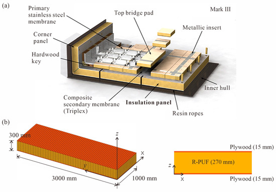
Figure 7. Insulation panel problem: (a) Typical configuration of an insulation panel (Mark III) [29]; (b) problem description with a 60 $\times$ 20 $\times$ 20 mesh of 8-node hexahedral 3D solid elements with 76,860 free DOFs.

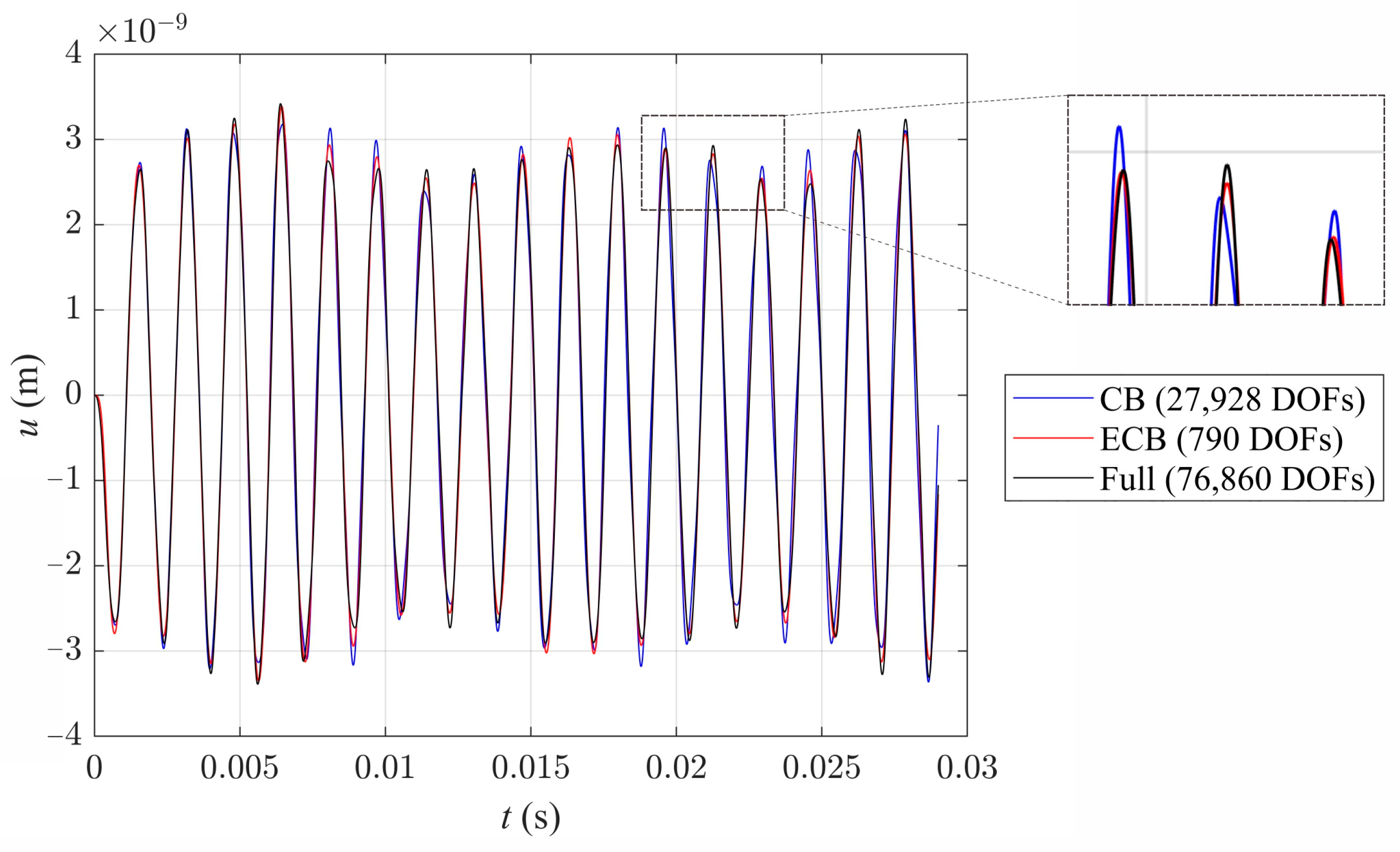
The finite element model consists of a 60 $\times$ 20 $\times$ 20 mesh of the standard 8-node hexahedral 3D solid elements with 76,860 free DOFs, as illustrated in Figure 7b. The simulation is conducted over a total time of 0.029 s with a time step of 1.45 $\times$ 10⁻⁵ s. The region of interest for partial back-transformation is defined as the DOFs at the load application region.

Table 4 provides detailed information on the CB and ECB reduced order models. Both models are configured with the same number of substructures, set to 128. As reduction methods generally require increased substructuring with larger model sizes or more DOFs, this example uses more substructuring than the first example. Table 4 shows that, with the same number of substructures, the ECB model achieves significantly greater DOF reduction than the CB model.

Table 4. Specifications of the CB and ECB reduced order models for the insulation panel problem. The full model has a total of 76,860 free DOFs.

	CB	ECB
Number of substructures	128	128
Number of dominant substructural normal modes	640 (=128 $\times$ 5)	640 (=128 $\times$ 5)
Interface boundary DOFs	27,288	-
Reduced interface boundary DOFs	-	150
Total reduced DOFs	27,928	790

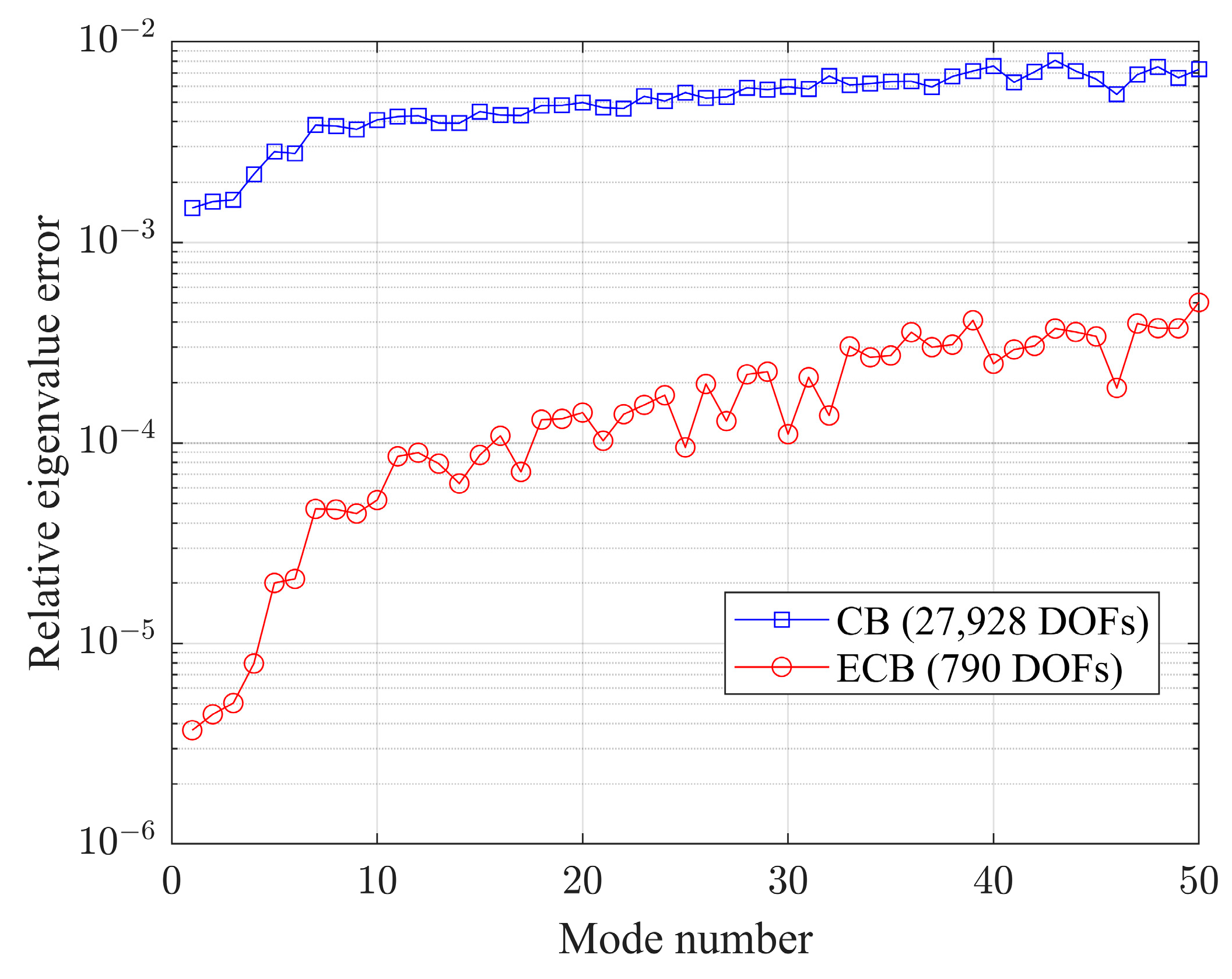
Figure 8 presents the relative eigenvalue errors for modes 1 to 50 for the CB and ECB reduced order models, with the full model results used as the reference. The ECB reduced order model achieves higher accuracy than the CB-reduced order model. Figure 9 illustrates the time history of $z$-direction displacement at the center point on the top surface. Table 5 presents the solution times for direct time-response analysis. Considering both solution accuracy and computation time, the ECB method is demonstrated to be remarkably powerful.

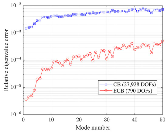
Figure 8. Relative eigenvalue errors of modes 1 to 50 for the insulation panel problem.

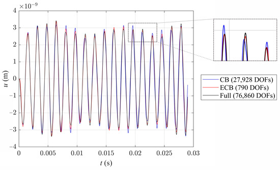
Figure 9. Displacement time history at the center point on the top surface for the insulation panel problem.

Table 5. Solution times of direct time-response analyses for the insulation panel problem (in seconds).

	Full Model	CB	ECB
Reduction	-	18.24	77.32
Newmark	226.11	189.59	0.68
Partial back-transformation	-	2.26	9.04
Total	226.11	210.09	87.03

4.3. Robot Arm

The last example considers a robot arm subjected to a harmonic loading, as shown in Figure 10a. The various parts comprising the robot are assumed to be rigidly connected, with their material properties unified as an elastic modulus of $2\times {10}^{11}\hspace{0.17em}\hspace{0.17em}{\mathrm{N}/\mathrm{m}}^2$, a Poisson’s ratio of 1/3, and a density of $7850\hspace{0.17em}\hspace{0.17em}{\mathrm{kg}/\mathrm{m}}^3$. A fixed support is applied to the face marked in red, as shown in Figure 10a, while a harmonic loading is uniformly distributed on the other red-marked face, with its total magnitude (unit: $\mathrm{N}$) defined as follows:

$$f(t)=30\times \left[\sin \left(10,000t\right)+\sin \left(20,000t\right)+\sin \left(30,000t\right)\right]\hspace{0.17em}.$$

(28)

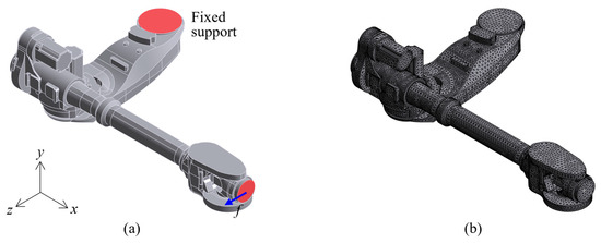
Figure 10. Robot arm problem: (a) problem description; (b) a mesh of 4-node tetrahedral 3D solid elements with 101,514 free DOFs.

The high-frequency harmonic loading discussed above approximates the conditions experienced by robot arms used in precision machining [30,31].

Figure 10b illustrates a finite element mesh generated using four-node tetrahedral 3D solid elements comprising 101,514 free DOFs. The simulation for this case is conducted over a total time of 1.4 $\times$ 10⁻³ s with a time step of 1.4 $\times$ 10⁻⁷ s. The region of interest for partial back-transformation is defined as the DOFs in the load application region.

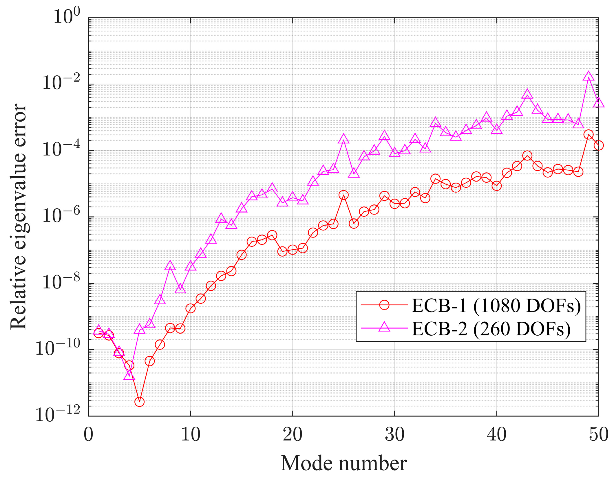
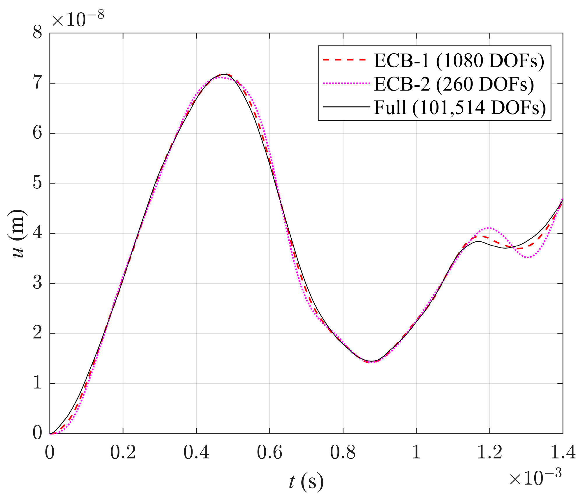
In this example, as summarized in Table 6, two ECB reduced order models are configured with varying reduced interface boundary DOFs, and their results are compared. Figure 11 presents the relative eigenvalue errors for modes 1 to 50 for the two ECB reduced order models, with the full model results used as the reference. Figure 12 presents the time history of $z$-direction displacement at the center point on the load application face. Table 7 presents the solution times for direct time-response analysis. This example again demonstrates the effectiveness of the ECB method in direct time-response analysis. However, as shown in Figure 12, a reduced order model with insufficient DOFs may lead to a loss of accuracy.

Table 6. Specifications of the two ECB reduced models for the robot arm problem. The full model has a total of 101,514 free DOFs.

	ECB-1	ECB-2
Number of substructures	32	32
Number of dominant substructural normal modes	480 (=32 $\times$ 15)	160 (=32 $\times$ 5)
Interface boundary DOFs	-	-
Reduced interface boundary DOFs	600	100
Total reduced DOFs	1080	260

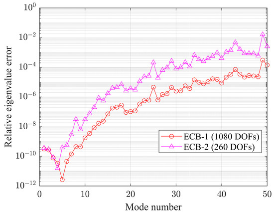
Figure 11. Relative eigenvalue errors of modes 1 to 50 for the robot arm problem.

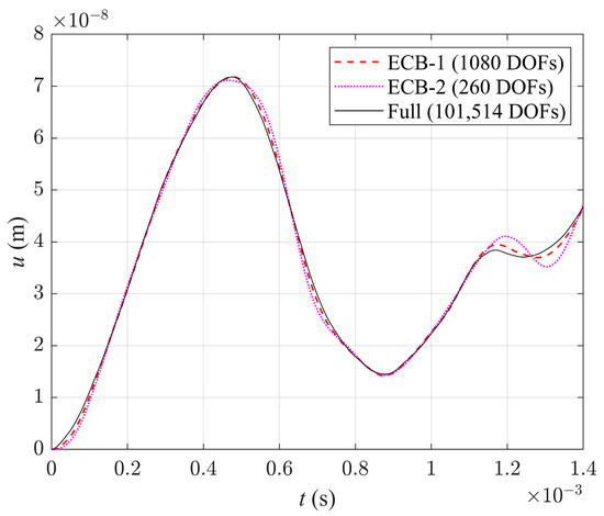
Figure 12. Displacement time history at the center point on the load application face for the robot arm problem.

Table 7. Solution times of direct time-response analyses for the robot arm problem (in seconds).

	Full Model	ECB-1	ECB-2
Reduction	-	137.69	41.73
Newmark	360.90	14.20	0.77
Partial back-transformation	-	5.40	1.64
Total	360.90	157.29	44.15

5. Conclusions

This study presented an application of the Enhanced Craig–Bampton (ECB) method for direct time-response analysis of finite element models. This research aimed to provide an effective strategy for reducing computational effort in dynamic analysis while ensuring accurate dynamic response predictions, achieved through the application of the ECB method with varying configurations of reduced order models. To complement this strategy, partial back-transformation was introduced to ensure that the analysis focused on targeted regions of finite element models identified as critical for practical design or analysis. The following key highlights differentiate this study from existing works and underline its contributions:

• Improved computational efficiency for direct time-response analysis: The proposed methodology demonstrated significant reductions in computational time through the optimized use of reduced order modeling. In Example 4.2, using the same number of substructures, the ECB method reduced the total degrees of freedom (DOFs) by approximately 98.97% compared to the full model and 97.17% compared to the CB-reduced order model, while achieving comparable accuracy in displacement results. Additionally, the ECB method reduced the total computational time by 58.57% compared to the CB method, showcasing its efficiency in dynamic analysis.
• Enhanced accuracy compared to the conventional CB method: By incorporating additional substructural modes and leveraging interface boundary reduction techniques, the ECB method outperformed the CB method in terms of both numerical accuracy and dynamic response precision.
• Practical applicability in engineering problems: The ECB method’s ability to target specific regions of interest makes it highly practical for complex engineering applications, such as transient analyses of large-scale structures in shipbuilding, offshore engineering, and mechanical systems.

Future work will extend this methodology to large-scale finite element models with millions of degrees of freedom [32,33]. Furthermore, upcoming studies will investigate advanced model reduction techniques, such as Adaptive Local Mode Synthesis (ALMS) and Enhanced ALMS, to achieve greater efficiency in transient analysis [34]. Additional innovations, including adaptive mode selection strategies, will also be explored.

References

- Craig, R.R., Jr.; Kurdila, A.J. Fundamentals of Structural Dynamics; John Wiley & Sons: Hoboken, NJ, USA, 2006. [Google Scholar]
- Bathe, K.J. Finite Element Procedures; Klaus-Jurgen Bathe: Watertown, MA, USA, 2006. [Google Scholar]
- Kaplan, M.F. Implementation of Automated Multilevel Substructuring for Frequency Response Analysis of Structures. Ph.D. Thesis, The University of Texas at Austin, Austin, TX, USA, 2001. [Google Scholar]
- Jokhio, G.A.; Izzuddin, B.A. A dual super-element domain decomposition approach for parallel nonlinear finite element analysis. Int. J. Comput. Methods Eng. Sci. Mech. 2015, 16, 188–212. [Google Scholar] [CrossRef]
- Hurty, W.C. Dynamic analysis of structural systems using component modes. AIAA J. 1965, 3, 678–685. [Google Scholar] [CrossRef]
- Craig, R.R., Jr.; Bampton, M.C. Coupling of substructures for dynamic analyses. AIAA J. 1968, 6, 1313–1319. [Google Scholar] [CrossRef]
- Benfield, W.A.; Hruda, R. Vibration analysis of structures by component mode substitution. AIAA J. 1971, 9, 1255–1261. [Google Scholar] [CrossRef]
- Ibrahimbegovic, A.; Wilson, E.L. Automated truncation of Ritz vector basis in modal transformation. J. Eng. Mech. 1990, 116, 2506–2520. [Google Scholar] [CrossRef]
- Craig, R.R., Jr. Substructure methods in vibration. J. Vib. Acoust. 1995, 117, 161–167. [Google Scholar] [CrossRef]
- Luo, K.; Hu, H.; Liu, C.; Tian, Q. Model order reduction for dynamic simulation of a flexible multibody system via absolute nodal coordinate formulation. Comput. Methods Appl. Mech. Eng. 2017, 324, 573–594. [Google Scholar] [CrossRef]
- Lee, J. A parametric reduced-order model using substructural mode selections and interpolation. Comput. Struct. 2019, 212, 199–214. [Google Scholar] [CrossRef]
- Baek, S.; Cho, M. The transient and frequency response analysis using the multi-level system condensation in the large-scaled structural dynamic problem. Struct. Eng. Mech. 2011, 38, 429–441. [Google Scholar] [CrossRef]
- Kim, J.G.; Lee, P.S. An enhanced Craig–Bampton method. Int. J. Numer. Methods Eng. 2015, 103, 79–93. [Google Scholar] [CrossRef]
- Boo, S.H.; Kim, J.H.; Lee, P.S. Towards improving the enhanced Craig-Bampton method. Comput. Struct. 2018, 196, 63–75. [Google Scholar] [CrossRef]
- George, A. Nested dissection of a rectangular finite element mesh. SIAM J. Numer. Anal. 1973, 10, 345–363. [Google Scholar] [CrossRef]
- Hendrickson, B.; Rothberg, E. Effective sparse matrix ordering: Just around the bend. In Proceedings of the Eighth SIAM Conference on Parallel Processing for Scientific Computing, Minneapolis, MN, USA, 10–12 March 1997. [Google Scholar]
- Karypis, G.; Kumar, V. METIS v4.0, a Software Package for Partitioning Unstructured Graphs, Partitioning Meshes, and Computing Fill-Reducing Orderings of Sparse Matrices; Technical Report; University of Minnesota: Minneapolis, MN, USA, 1998. [Google Scholar]
- Bennighof, J.K.; Lehoucq, R.B. An automated multilevel substructuring method for eigenspace computation in linear elastodynamics. SIAM J. Sci. Comput. 2004, 25, 2084–2106. [Google Scholar] [CrossRef]
- Yang, C.; Gao, W.; Bai, Z.; Li, X.S.; Lee, L.Q.; Husbands, P.; Ng, E. An algebraic substructuring method for large-scale eigenvalue calculation. SIAM J. Sci. Comput. 2005, 27, 873–892. [Google Scholar] [CrossRef]
- Boo, S.H.; Lee, P.S. A dynamic condensation method using algebraic substructuring. Int. J. Numer. Methods Eng. 2017, 109, 1701–1720. [Google Scholar] [CrossRef]
- Boo, S.H.; Lee, P.S. An iterative algebraic dynamic condensation method and its performance. Comput. Struct. 2017, 182, 419–429. [Google Scholar] [CrossRef]
- Rixen, D.J. Interface reduction in the Dual Craig-Bampton method based on dual interface modes. Link. Models Exp. 2011, 2, 311–328. [Google Scholar]
- Xi, C.; Zheng, H. Improving the generalized Bloch mode synthesis method using algebraic condensation. Comput. Methods Appl. Mech. Eng. 2021, 379, 113758. [Google Scholar] [CrossRef]
- Zhu, X.; Xi, C.; Zheng, H. An improvement of generalized Bloch mode synthesis method-based model order reduction technique for band-structure computation of periodic structures. Comput. Struct. 2023, 281, 107013. [Google Scholar] [CrossRef]
- Junge, M.; Brunner, D.; Becker, J.; Gaul, L. Interface-reduction for the Craig–Bampton and Rubin method applied to FE–BE coupling with a large fluid–structure interface. Int. J. Numer. Methods Eng. 2009, 77, 1731–1752. [Google Scholar] [CrossRef]
- Ko, Y.; Lee, P.S.; Bathe, K.J. A new MITC4+ shell element. Comput. Struct. 2017, 182, 404–418. [Google Scholar] [CrossRef]
- Choi, H.G.; Lee, P.S. The simplified MITC4+ shell element and its performance in linear and nonlinear analysis. Comput. Struct. 2023, 290, 107177. [Google Scholar] [CrossRef]
- Rezaiee-Pajand, M.; Masoodi, A.R.; Rajabzadeh-Safaei, N. Nonlinear vibration analysis of carbon nanotube reinforced composite plane structures. Steel Compos. Struct. 2019, 30, 493–516. [Google Scholar]
- Nho, I.S.; Ki, M.S.; Kim, S.C.; Lee, J.H.; Kim, Y. Sloshing Impact Response Analysis for Insulation System of LNG CCS Considering Elastic Support Effects of Hull Structures. J. Ocean Eng. Technol. 2017, 31, 357–363. [Google Scholar] [CrossRef]
- Slamani, M.; Chatelain, J.F. Assessment of the suitability of industrial robots for the machining of carbon-fiber reinforced polymers (CFRPs). J. Manuf. Process. 2019, 37, 177–195. [Google Scholar] [CrossRef]
- Kim, D.C.; Seo, J.; Park, H.W. Dynamic performance of industrial robots in the secondary carbon fiber-reinforced plastics machining. J. Manuf. Process. 2023, 103, 120–135. [Google Scholar] [CrossRef]
- Lee, C.; Park, J. Preconditioning for finite element methods with strain smoothing. Comput. Math. Appl. 2023, 130, 41–57. [Google Scholar] [CrossRef]
- Lee, C.; Moon, M.; Park, J. A gradient smoothing method and its multiscale variant for flows in heterogeneous porous media. Comput. Methods Appl. Mech. Eng. 2022, 395, 115039. [Google Scholar] [CrossRef]
- Rachowicz, W.; Zdunek, A. Automated multi-level substructuring (AMLS) for electromagnetics. Comput. Methods Appl. Mech. Eng. 2009, 198, 1224–1234. [Google Scholar] [CrossRef]
Disclaimer/Publisher’s Note: The statements, opinions and data contained in all publications are solely those of the individual author(s) and contributor(s) and not of MDPI and/or the editor(s). MDPI and/or the editor(s) disclaim responsibility for any injury to people or property resulting from any ideas, methods, instructions or products referred to in the content. |
© 2025 by the authors. Licensee MDPI, Basel, Switzerland. This article is an open access article distributed under the terms and conditions of the Creative Commons Attribution (CC BY) license (https://creativecommons.org/licenses/by/4.0/).