Interpolating Triangular Meshes Using a Non-Uniform, Non-Stationary Loop Subdivision

Abstract

This paper presents a novel non-uniform, non-stationary Loop subdivision that directly interpolates arbitrary initial triangular meshes. This subdivision is derived by assigning distinct parameters for “vertex-point” and “edge-point” generation within the stencils of a uniform, non-stationary Loop subdivision. This underlying uniform, non-stationary scheme is obtained based on a suitably chosen iterative process. Crucially, we derive the limit positions of the initial points under this non-uniform scheme and decrease the assigned parameters to a single shape parameter when interpolating the initial mesh. Compared with the existing methods interpolating the initial mesh using approximating subdivision, this new one achieves interpolation in finite steps and without any additional adjustment to the initial mesh or subdivision rules. Several numerical examples are given to show the scheme’s interpolation accuracy and shape control capabilities.

1. Introduction

Subdivision schemes are widely used in fields like computer graphics, animation and games due to their efficiency in generating smooth surfaces, numerical stability and implementation simplicity. In general, these subdivision schemes are categorized as approximating and interpolatory schemes. While the interpolatory schemes inherently interpolate the initial mesh, approximating schemes offer superior smoothness and better reflect the shape of the initial mesh. Classic approximating subdivision schemes include Loop subdivision [1] and Catmull–Clark subdivision [2]. For more details about subdivision, please refer to [3].

Due to the advantages of approximating subdivision, there is significant interest in adapting them to interpolate the initial mesh. In connection with this topic, Sun and Lu [4] gave a progressive interpolation method, while Zheng and Cai [5] proposed a two-phase subdivision to interpolate the initial mesh based on the Catmull–Clark subdivision. Deng and Wang [6] gave an interesting way to interpolate the triangular mesh using the limit positions of initial points under Loop subdivision. Additionally, for Loop subdivision, Cheng et al. [7] iteratively upgrade the vertices of initial mesh to generate a new mesh whose limit surface interpolate the initial mesh. Hamza et al. [8] proposed new progressive iterative approximation formats for Loop and Catmull–Clark subdivision based on the Hermitian and skew-Hermitian splitting iteration technique to interpolate the initial mesh. Other relevant works include [9,10] and the references therein.

However, there is a common limitation of the methods in the above works, i.e., they cannot interpolate the initial mesh directly. This means that they require additional adjustments to either the initial mesh or the subdivision rules themselves. Therefore in this paper, we try to present a new way for the direct interpolation of triangular meshes using a kind of non-uniform, non-stationary variant of Loop subdivision. In fact, compared with the stationary schemes used for initial mesh interpolation, non-uniform, non-stationary schemes generate richer function spaces and offer enhanced shape control, which motivates our approach. Such examples include the non-stationary, generalized Loop subdivision by Badoual et al. [11] constructed for chemical imaging and other related works like [12,13,14,15,16] and the references therein. Here, we point out that, for the triangular mesh containing vertices that do not have the same valence, the scheme given in [16] only interpolates the initial vertices sharing the same valence but cannot interpolate all of the initial vertices.

In fact, the new non-uniform, non-stationary Loop subdivision is obtained in two steps. First, we construct a non-stationary Loop subdivision based on a suitable iteration. Then, we derive the desired non-uniform scheme by strategically parameterizing the initial points inspired by [16] (see Section 3.3 for differences) to modify the corresponding stencils. For such a non-uniform, non-stationary subdivision, we derive the limit positions of the initial control points. Interpolation of the initial mesh is then achieved by setting the limit positions equal to the initial points. Crucially, this reduces the number of parameters to only one, which actually governs edge point generation and controls the shape of the final interpolating surfaces.

Compared with other methods for initial mesh interpolation via approximating schemes, besides locality and easiness in use, our approach also offers the following advantages:

(1) Direct interpolation: The initial mesh is interpolated using this new method directly, eliminating the need for additional adjustments to the initial mesh or subdivision rules.

(2) Ease of shape control: For the final limit surface interpolating the initial mesh, a single free parameter allows intuitive adjustments of the corresponding shape.

(3) Finite-step interpolation: Our new approach achieves practical interpolation with finite steps of subdivision.

We point out that our method advances reconstruction in fields like computer graphics and imaging. In such fields, reconstruction often relies on integral constraints or unstructured point clouds. By directly interpolating arbitrary triangular meshes—a common representation for scattered 3D data—our method bypasses costly preprocessing, bridging subdivision theory with practical reconstruction demands in graphics and imaging. The single-shape parameter offers intuitive control over surface features, benefiting applications like point-cloud upsampling [17], which is similar to the enriched Crouzeix–Raviart approach [18] using weighted polynomial bases to handle integral data. The finite-step interpolation capability also contrasts with iterative optimization methods, potentially offering computational advantages for certain scenarios. All of these position this new method as a competitive alternative for applications where topological consistency is critical like biomedical surface modeling.

The rest of this paper is organized as follows. Section 2 details the construction of the new non-uniform, non-stationary Loop subdivision. Section 3 is devoted to the limit position of initial points and presents the interpolation framework. In Section 4, we illustrate some examples to show the interpolation accuracy and shape control capabilities of the new non-uniform, non-stationary Loop subdivision scheme. Section 5 concludes this paper.

2. The Non-Uniform, Non-Stationary Loop Subdivision

In this section, we construct the new non-uniform, non-stationary Loop subdivision. To this purpose, we first derive a uniform, non-stationary Loop subdivision. Based on this non-stationary Loop subdivision, we obtain the desired non-uniform, non-stationary Loop subdivision.

We point out that, given an initial data sequence ${\mathit{q}}^0=\{q_{\mathit{\alpha }}^0,\mathit{\alpha }\in {\mathbb{Z}}^2\}\in l_0\left({\mathbb{Z}}^2\right)$, the subdivision schemes in this paper are of the following type:

$${\left(S_{{\mathit{a}}^k}{\mathit{q}}^k\right)}_{\mathit{\alpha }}=q_{\mathit{\alpha }}^{k+1}=\sum _{\mathit{\beta }\in {\mathbb{Z}}^2}{a}_{\mathit{\alpha }-2\mathit{\beta }}^k{q}_{\mathit{\beta }}^k,\mathit{\alpha }\in {\mathbb{Z}}^2,$$

where $S_{{\mathit{a}}^k}$ is the k-level subdivision operator, and the sequence ${\mathit{a}}^k=\{a_{\mathit{\alpha }}^k,\mathit{\alpha }\in {\mathbb{Z}}^2\}$ is the k-level mask with finite support. We denote this scheme by ${\left\{S_{{\mathit{a}}^k}\right\}}_{k\ge 0}$, and the corresponding k-level symbol is the Laurent polynomial $a^k\left(\mathit{z}\right)={\displaystyle \sum _{\mathit{\alpha }\in {\mathbb{Z}}^2}}{a}_{\mathit{\alpha }}^k{\mathit{z}}^{\mathit{\alpha }}$.

2.1. The Uniform, Non-Stationary Loop Subdivision

Now we derive the uniform, non-stationary Loop subdivision scheme, which is denoted by ${\left\{S_{{\mathit{a}}^k}\right\}}_{k\ge 0}$.

In fact, such a non-stationary scheme is based on a suitable iteration process. For this, we denote by $\phi \left(x\right)=x/5$ the iteration function with the fixed point $x^{*}=0$, and thus the corresponding iteration process can be described by

$$v^{k+1}=\phi \left(v^k\right)=v^k/5,v^0\in \mathbb{R}.$$

Then, in the regular part of the mesh, the non-stationary Loop subdivision ${\left\{S_{{\mathit{a}}^k}\right\}}_{k\ge 0}$ is characterized in terms of the k-level mask

$${\mathit{a}}^k=\left(\begin{array}{ccccc}0& 0& v^{k+1}/2+1/16& v^{k+1}+1/8& v^{k+1}/2+1/16\\ 0& v^{k+1}+1/8& 3/8-v^{k+1}& 3/8-v^{k+1}& v^{k+1}+1/8\\ v^{k+1}/2+1/16& 3/8-v^{k+1}& 5/8-3v^{k+1}& 3/8-v^{k+1}& v^{k+1}/2+1/16\\ 1/8+v^{k+1}& 3/8-v^{k+1}& 3/8-v^{k+1}& 1/8+v^{k+1}& 0\\ 1/16+v^{k+1}/2& 1/8+v^{k+1}& 1/16+v^{k+1}/2& 0& 0\end{array}\right).$$

(1)

For the subdivision rules in the neighborhood of an extraordinary point of valence n, with $v^{k+1}=v^k/5$, the corresponding local subdivision matrix ${\tilde{S}}^k$ is

$${\tilde{S}}^k=\left(\begin{array}{cc}1-n{\alpha }^k& {\mathit{\alpha }}^k\\ {\mathit{\beta }}^k& {\tilde{\mathit{B}}}_j^k\end{array}\right),$$

(2)

where

$${\alpha }^k=[5/8+v^{k+1}-{(3/8+\cos (2\pi /n)/4)}^2]/n,{\mathit{\alpha }}^k=({\alpha }^k,\cdots ,{\alpha }^k),{\mathit{\beta }}^k={(b_0^k,b_1^k\cdots ,b_{n-1}^k,b_n^k)}^{\top },$$

and ${\tilde{\mathit{B}}}^k$ is the $n\times n$ circulant matrix ${\tilde{\mathit{B}}}^k=circ(b_0^k,b_1^k,\cdots ,b_{n-1}^k)$ with $b_0^k=3/8-v^{k+1},b_1^k=v^{k+1}+1/8,b_2^k=\cdots =b_{n-2}^k=0,b_{n-1}^k=h\left(v^{k+1}\right)$. The corresponding stencils to generate a ‘vertex’ point (with valence $n=6$ and $n\ne 6$) and an ‘edge’ point are as in Figure 1.

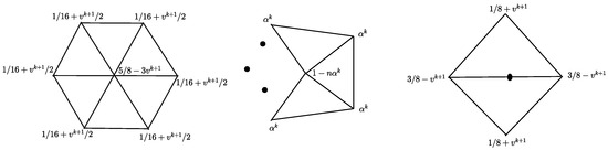
Figure 1. Stencils for the scheme ${\left\{S_{{\mathit{a}}^k}\right\}}_{k\ge 0}$ to generate a ‘vertex’ point with valence $n=6$ (left) and $n\ne 6$ (middle) and an ‘edge’ point (right).

Remark 1. 

When $v^0=0$, we have $v^k=0$ for all $k\in {\mathbb{N}}_0$. In this case, the k-level mask in (1) and the local subdivision matrix in (2) reduce to their stationary counterparts from the classic Loop subdivision. Therefore, since $\underset{k\to \infty }{\lim }{v}^k=0$, the scheme ${\left\{S_{{\mathit{a}}^k}\right\}}_{k\ge 0}$ asymptotically approaches the standard Loop subdivision $S_{\mathit{a}}$ as $k\to \infty$.

The smoothness of this uniform, non-stationary scheme in the regular part of the mesh can be done in a similar way to [14], yielding the following result.

Theorem 1. 

The new non-stationary Loop subdivision ${\left\{S_{{\mathit{a}}^k}\right\}}_{k\ge 0}$ is $C^2$-convergent in the regular part of the mesh.

The proof of Theorem 1 is given in Appendix A. Now we give the result on the smoothness of ${\left\{S_{{\mathit{a}}^k}\right\}}_{k\ge 0}$ near the extraordinary points. In fact, we have the following result.

Theorem 2. 

The scheme ${\left\{S_{{\mathit{a}}^k}\right\}}_{k\ge 0}$ is tangent plane continuous at the limit position of the extraordinary point of valence n.

The proof of Theorem 2 is given in Appendix B.

2.2. The Non-Uniform, Non-Stationary Loop Subdivision

Building upon the non-stationary scheme ${\left\{S_{{\mathit{a}}^k}\right\}}_{k\ge 0}$, we now derive the desired non-uniform, non-stationary Loop subdivision scheme.

In fact, on the topic of constructing the non-uniform subdivision schemes, there have been several related works, such as the proposed schemes in [19,20,21]. Yet, different from these works, to give the non-uniform version of the scheme ${\left\{S_{{\mathit{a}}^k}\right\}}_{k\ge 0}$ in this paper, we use a way similar to the local control discussion in [14].

To be more specific, we achieve non-uniformity by assigning distinct initial parameters: setting the initial parameter $v_{i,n}^0\in \mathbb{R}$ to the ith initial point with valence n and setting $v_e^0\in \mathbb{R}$ as the initial parameter for the new edge point generation. As for the correspondence of the points in the coarse mesh and the ones in the refined mesh, we use the iteration $v_{i,n}^{k+1}=v_{i,n}^k/5$ for the parameters of new vertex points and $v_e^{k+1}=v_e^k/5$ for the parameter of new edge points. Then, the stencils in Figure 1 are then modified by replacing $v^{k+1}$ with $v_{i,n}^{k+1}$ in the vertex point generation stencil (left of Figure 1), substituting ${\alpha }^k$ with ${\alpha }_i^k=\alpha +v_{i,n}^k/n$ (middle of Figure 1) and replacing $v^{k+1}$ with $v_e^{k+1}$ (right of Figure 1). In this way, we obtain the desired non-uniform version of the scheme ${\left\{S_{{\mathit{a}}^k}\right\}}_{k\ge 0}$.

Here, we note that this non-uniform scheme differs from the one proposed in [16]. The key distinction lies in the parameter assigned for the initializing edge-point generation. The assigned initial parameter in this paper is a distinct parameter $v_e^0$, while the scheme in [16] actually uses the average of the parameters assigned to the initial points. The advantage of introducing the additional parameter $v_e^0$ is that it provides greater flexibility in initial mesh interpolation, enabling the interpolation of different kinds of triangular meshes and adjustment of the shape of the corresponding limit surfaces, which cannot be achieved using the scheme in [16].

For this, we give a table for comparison. Table 1 lists the main differences between the new non-uniform scheme in this paper and the uniform and non-uniform schemes in [16]. In Table 1, $v_{i,n}^0$ and $v_e^0$ are the initial parameters assigned for the i th initial point (with valence n) and edge point generation, and $M^0$ is the initial control mesh. Additionally, Scheme 1, Scheme 2 and Scheme 3 are the non-uniform, non-stationary scheme in this paper and the non-uniform and uniform ones in [16], respectively.

Table 1. Comparison between different non-stationary schemes.

	${\mathit{v}}_{\mathit{i},\mathit{n}}^0$	${\mathit{v}}_{\mathit{e}}^0$	Interpolate ${\mathit{P}}_{\mathit{n}}^0$	Interpolate ${\mathit{M}}^0$
Scheme 1	depend on $v_e^0$	Free	Yes	Yes
Scheme 2	free	Average of $v_{i,n}^0$	Yes	No
Scheme 3	$v^0$	$v^0$	No	No

3. Triangular Mesh Interpolation

In this section, we address the interpolation of triangular meshes using the new non-uniform, non-stationary Loop scheme. For this, we first derive the limit positions of initial points.

3.1. Limit Positions of Initial Points

In fact, for the classic Loop subdivision $S_{\mathit{a}}$, the limit position of initial points has been obtained as ([17])

$$P_0^{\infty }=(1-n\gamma )P_0^0+\gamma \sum _{i=1}^n{P}_i^0,$$

(3)

where $\gamma ={(3/\left(8\alpha \right)+n)}^{-1}$. Now we generalize this result to give the limit positions of initial points for the new non-uniform, non-stationary Loop scheme in the spirit of the push-back method ([22]), as shown in the following result.

Theorem 3. 

Let $P_{0,n}^0$ be the initial point with valence n with the $1$-ring neighborhood points $P_j^0$ ($j=1,\cdots ,n$) and let $v_{0,n}^0$ and $v_e^0$ be the initial parameters for vertex points generation with valence n and edge points generation, respectively. Then, the limit position of $P_{0,n}^0$ obtained by the non-uniform, non-stationary Loop subdivision is

$$P_{0,n}^{\infty }=(1-n\lambda )P_{0,n}^0+\lambda \sum _{j=1}^n{P}_j^0,$$

(4)

where

$$\lambda =\left\{\begin{array}{c}\sum _{k=0}^{\infty }{\alpha }_0^k\prod _{j=1}^k(\left(v_e^0-v_{0,n}^0\right)/5^j+{(3/8+\cos (2\pi /n)/4)}^2),n\ne 6,\hfill \\ \sum _{k=0}^{\infty }(1/16+0.5\ast v_{0,n}^0/5^{k+1})\prod _{j=1}^k(1/4+\left(v_e^0-3v_{0,n}^0\right)/5^j),n=6.\hfill \end{array}\right.$$

(5)

The proof of Theorem 3 is given in Appendix C.

Remark 2. 

When all the initial parameters $v_{i,n}^0$ and $v_e^0$ choose the same value $v^0$, this non-uniform, non-stationary scheme reduces to the uniform, non-stationary scheme ${\left\{S_{{\mathit{a}}^k}\right\}}_{k\ge 0}$. Then, for the corresponding limit positions of initial points, λ in (4) becomes

$$\lambda =\left\{\begin{array}{c}{(3/\left(8\alpha \right)+n)}^{-1}+v^0{(35/8+n\alpha )}^{-1}/n,n\ne 6,\hfill \\ \sum _{k=0}^{\infty }(1/16+0.5\ast v^0/5^{k+1})\prod _{j=1}^k(1/4-2v^0/5^j),n=6.\hfill \end{array}\right.$$

(6)

If we further set $v^0=0$, then λ in (6) reduces to ${(3/\left(8\alpha \right)+n)}^{-1}$, which is actually γ in (3) in the case of classic Loop subdivision.

3.2. Interpolating an Initial Point

Now building upon the limit positions of initial points established in Theorem 3, we address the initial point interpolation.

In fact, Theorem 3 reveals that, for the initial point $P_{0,n}^0$, the coefficient $\lambda$ depends on $v_e^0,v_{0,n}^0$ and the valence n. Now define $P^0:={\displaystyle \frac{1}{n}}{\displaystyle \sum _{j=1}^n}{P}_j^0$ as the centroid of the corresponding adjacent vertices, then the limit position $P_{0,n}^{\infty }$ in (4) can be rewritten as

$$\begin{array}{cc}\hfill P_{0,n}^{\infty }& =n\lambda P^0+(1-n\lambda )P_{0,n}^0.\hfill \end{array}$$

This formulation demonstrates that the limit position $P_{0,n}^{\infty }$ actually lies on the line crossing $P_{0,n}^0$ and the center of its 1-ring neighborhood points, i.e., $P^0$. It could be proved that, for each $\lambda \in \mathbb{R}$, there exists parameters $v_e^0,v_{0,n}^0\in \mathbb{R}$ satisfying (4). Consequently, this non-uniform scheme theoretically interpolates all the points lying on such a line, as shown in Figure 2.

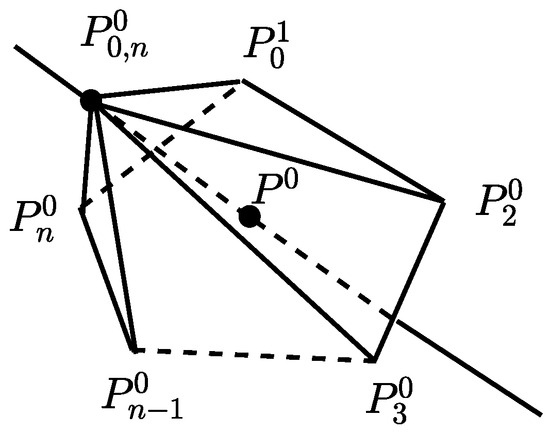
Figure 2. The line crossing $P_{0,n}^0$ and the center of its 1-ring neighborhood points.

To interpolate some point P on such a line crossing $P_{0,n}^0$ and the center of its 1-ring neighborhood, we only need to get the corresponding initial values of $v_{i,n}^0,v_e^0$. To this purpose, we rewrite the point P in the form of (4), i.e., $P=n\overline{\lambda }{P}^0+(1-n\overline{\lambda })P_0^0$. Then, by letting $P_0^{\infty }=P$, we get the value s of $\overline{\lambda }$, and solving $\lambda =s$ for the parameters gives the required $v_{i,n}^0,v_e^0$ (see Section 3.3 for details).

In particular, to interpolate the initial point $P_{0,n}^0$, we let the corresponding limit point $P_{0,n}^{\infty }=P_{0,n}^0$, which can be obtained with $\lambda =0$. Thus, to interpolate an initial mesh with n points of m distinct vertex valences, we need to solve a system of m equations with $m+1$ unknowns (i.e., $v_{i,n}^0$ and $v_e^0$). As a result, there is only one free parameter left, which we designate as $v_e^0$. The parameters $v_{i,n}^0$ then become valence dependent functions of $v_e^0$. Consequently, vertices with valence n share the same $v_{i,n}^0$ value. In other words, $v_{i,n}^0$ actually depends only on the valence n and $v_e^0$. Thus, we rewrite the parameter $v_{i,n}^0$ as $v_n^0$ in the following sections. For the free parameter $v_e^0$, it actually controls the shape of the limit surface and is the so-called shape parameter. In this way, this non-uniform scheme enables simultaneous interpolation of the initial mesh and flexible adjustment of the shape of the limit surfaces.

Remark 3. 

We can also use the iteration coming from the generation of exponential polynomials, i.e., $\phi \left(v^{k+1}\right)=\sqrt{v^k/2+1/2}$ with $v^0\in (-1,\infty )$ and obtain the corresponding limit positions of initial points. Yet, the corresponding scheme cannot reach all the points on the line crossing $P_{0,n}^0$ and the center of its 1-ring neighborhood points. In particular, the initial point $P_{0,n}^0$ cannot be interpolated since this interpolation needs λ in (4) to be 0, which is impossible for $v^0\in (-1,\infty )$.

3.3. Triangular Mesh Interpolation

Now we generate surfaces that interpolate the triangular meshes using the new non-uniform, non-stationary Loop subdivision.

Note that, as established in Section 3.2, to interpolate initial points with valence n, we need to solve the equation

$$\sum _{i=0}^{\infty }{\alpha }_0^i\prod _{j=1}^i({\displaystyle \frac{v_e^0+v_n^0}{5^j}}+{(3/8+\cos (2\pi /n)/4)}^2)=0,$$

(7)

for the parameters $v_e^0$ and $v_n^0$. This means that to interpolate a triangular mesh with points $P_0,\cdots ,P_n$ of m distinct valences, we need to solve a system of m equations and $m+1$ unknowns, as stated in Section 3.2. Following our earlier approach, we set the free parameter to be $v_e^0$, making the valence-specific parameters $v_n^0$ dependent on $v_e^0$.

The system in (7) contains an infinite series; thus, for such a system, we actually solve a truncated version yet with a controllable error bound (easier to control than the subdivision depth). Specifically speaking, for practical computation after k subdivision steps, we solve

$$\sum _{i=0}^k{\alpha }_0^i\prod _{j=1}^i({\displaystyle \frac{v_e^0+v_n^0}{5^j}}+{(3/8+\cos (2\pi /n)/4)}^2)=0.$$

(8)

When given a certain value of $v_e^0$, the corresponding value of $v_n^0$ can be obtained numerically (i.e., using software like Matlab R2018b). In addition, from (8) and the proof of Theorem 1, we have

$$P_0^{k+1}-P_0^0=\sum _{i=0}^k{\alpha }_0^i\prod _{j=1}^i({\displaystyle \frac{v_e^0+v_n^0}{5^j}}+{(3/8+\cos (2\pi /n)/4)}^2)A_0^0.$$

(9)

Thus, as $k\to \infty$, ${\displaystyle \sum _{i=0}^k}{\alpha }_0^i{\displaystyle \prod _{j=1}^i}({\displaystyle \frac{v_e^0+v_n^0}{5^j}}+{(3/8+\cos (2\pi /n)/4)}^2)$ tends to $\lambda$. Combining (8) and (9), the approximate values of the parameters $v_e^0$ and $v_n^0$ satisfying (8) make $P_0^{k+1}-P_0^0=0$. Thus, $P_0^0$ is interpolated after k steps of subdivision. This means that all the initial points (thus, the initial mesh) can be interpolated after k steps of subdivision. We point out that this is different from the existing methods fundamentally to interpolate the initial mesh using approximate subdivision.

Table 2 compares the new method for interpolation in this paper with other ones. In Table 2, adjustment 1 means the adjustment of subdivision rules, while adjustment 2 means the adjustment of the initial control mesh.

Table 2. Comparison between different methods for interpolation using Loop subdivision.

Items	Adjustment 1	Adjustment 2	Shape Control	Subdivision Steps
The new method	No	No	Yes	Finite
The method in [6]	Yes	No	Yes	Infinite
The method in [7]	No	Yes	No	Infinite

For this non-uniform scheme, we state in the Remark at the end of Appendix A for the smoothness in the regular part of the mesh and in the Remark at the end of Appendix B for the convergence near extraordinary points.

4. Examples

We now present some examples to illustrate the performance of this new non-uniform, non-stationary Loop subdivision. Before that, we first recall the definition of Hausdorff distance.

Let A and B denote two sets of points. Then, the Hausdorff distance between them is defined as

$$H(A,B)=\max \left(h\right(A,B),h(B,A\left)\right),$$

(10)

where

$$h(A,B)=\underset{a\in A}{\max }\{\underset{b\in B}{\min } \left|\right|a-b\left|\right|\},h(A,B)=\underset{b\in B}{\max }\{\underset{a\in A}{\min } \left|\right|a-b\left|\right|\},$$

and $\left|\right|·\left|\right|$ is the Euclidean distance.

Example 1. 

Consider the initial mesh in Figure 3 (leftmost) with initial points $(10,10,10),$$(-100,10,-10)$, $(-100,-10,10),$ and $(10,-10,-10)$(labeled by $\diamond$). Note that all the points of this initial mesh have valence 3. Then, to interpolate this mesh, by Theorem 3, we need to solve the following equation:

$$\sum _{k=0}^{\infty }(5/8+v_3^{k+1}-{(3/8+\cos (2\pi /3)/4)}^2)\prod _{j=1}^k(\left(v_e^0-v_3^0\right)/5^j+{(3/8+\cos (2\pi /3)/4)}^2)=0,$$

(11)

where $v_3^{k+1}$ is derived from $v_3^0$ through the parameter evolution $v_3^{k+1}={\displaystyle \frac{v_3^k}{5}}$. In (11), $v_e^0$ is the free parameter, and thus $v_3^0$ depends on $v_e^0$. By solving (12) with different values of $v_e^0$ and a truncation of 7, i.e.,

$$\sum _{k=0}^7(5/8+v_3^{k+1}-{(3/8+\cos (2\pi /3)/4)}^2)\prod _{j=1}^k(\left(v_e^0-v_3^0\right)/5^j+{(3/8+\cos (2\pi /3)/4)}^2)=0,$$

(12)

we obtain the corresponding values of $v_3^0$. Here, the chosen $v_e^0$ and the obtained $v_3^0$ are $(v_e^0,v_3^0)=(-1,-4.89),(-1.3,-4.57),(-1.6,-4.28)$. With these parameters, we obtain the meshes after seven subdivision steps which interpolates the initial mesh as shown in Figure 3 (the right three meshes).

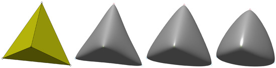
Figure 3. The meshes generated by the new non-uniform scheme starting from the initial mesh (leftmost) with $v_e^0=-1,-1.3,-1.6$ (left to right for the 3 surfaces on the right) after 7 steps of subdivision.

From Figure 3, it can be seen that with different values of $v_e^0$, the obtained meshes indeed interpolate the initial mesh while providing the shape control over the corresponding meshes. Table 3 shows the Hausdorff distance between the initial mesh and the obtained meshes. From Table 3, we see the change of the Hausdorff distance with the change of $v_e^0$.

Table 3. The Hausdorff distance (hd) between the initial mesh and the meshes obtained after 7 steps of subdivison with different $v_e^0$.

$v_e^0$	−1	−1.1	−1.3	−1.6
hd	56.3443	55.9023	55.9175	56.0911

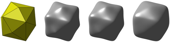
Example 2. 

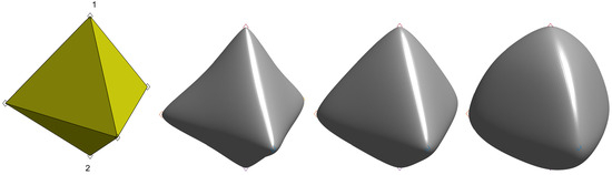
Now we give an example showing the interpolation of initial mesh with multiple vertex valences. Consider the initial mesh in Figure 4 (leftmost) with the points $(0,0,0),(2,0,0),(1,\sqrt{3},0),$$(1,\sqrt{3}/3,1),(1,\sqrt{3}/3,-1/2)$. Note that the vertices labeled 1 and 2 have valence 3 and the other three points have valence 4. To interpolate this initial mesh, by Theorem 3, we solve the valence-dependent system to find the initial parameters $v_3^0$ and $v_4^0$ with respect to the points with valence 3 and 4, i.e.,

$$\left\{\begin{array}{c}\sum _{k=0}^{\infty }(5/8+v_3^{k+1}-{(3/8+\cos (2\pi /3)/4)}^2)\prod _{j=1}^k(\left(v_e^0-v_3^0\right)/5^j+{(3/8+\cos (2\pi /3)/4)}^2)=0,\hfill \\ \sum _{k=0}^{\infty }(5/8+v_4^{k+1}-{(3/8+\cos (2\pi /4)/4)}^2)\prod _{j=1}^k(\left(v_e^0-v_4^0\right)/5^j+{(3/8+\cos (2\pi /4)/4)}^2)=0.\hfill \end{array}\right.$$

(13)

Figure 4. Meshes obtained by this new non-uniform scheme starting from the initial mesh (leftmost) with $v_e^0=-1,-1.3,-1.7$ (left to right for the 3 surfaces on the right) after 7 steps of subdivision.

Here, we choose $v_e^0=-1,-1.3,-1.7$. Then, by solving (14) with a truncation of 7 numerically, i.e., solving

$$\left\{\begin{array}{c}\sum _{k=0}^7(5/8+v_3^{k+1}-{(3/8+\cos (2\pi /3)/4)}^2)\prod _{j=1}^k(\left(v_e^0-v_3^0\right)/5^j+{(3/8+\cos (2\pi /3)/4)}^2)=0,\hfill \\ \sum _{k=0}^7(5/8+v_4^{k+1}-{(3/8+\cos (2\pi /4)/4)}^2)\prod _{j=1}^k(\left(v_e^0-v_4^0\right)/5^j+{(3/8+\cos (2\pi /4)/4)}^2)=0.\hfill \end{array}\right.$$

(14)

the values of $v_3^0,v_4^0$ are $(v_3^0,v_4^0)=(-4.89,-4.25),(-4.57,-3.97),(-4.17,-3.62)$. With such parameters, we have the corresponding meshes interpolating the initial mesh in Figure 4 (right three meshes) after seven steps of subdivision.

We point out that, although the parameter $v_e^0$ can theoretically choose any value in $\mathbb{R}$ (see Section 3.2) to interpolate the initial mesh with relatively flat surface, we choose $v_e^0<0$ as shown in Figure 3 and Figure 4 and other examples. Additionally, from Figure 3 and Figure 4, it can be seen that, with different values of $v_e^0$, the initial mesh can indeed be interpolated. Meanwhile, Figure 3 and Figure 4 reveal the effect of $v_e^0$ on the shape of the limit surfaces, i.e., when $v_e^0<0$ decreases, the corresponding limit surfaces interpolating the initial mesh expand, thus visually becoming more convex. This is because when the free parameter $v_e^0<0$ decreases, the new edge point moves away from their corresponding edge (outwards the initial mesh). Yet, if we generate the reasonable flat and visually convex surfaces, we choose $v_e^0$ between $-1$ and $-2$, as shown in Figure 5, which implies that when $v_e^0<-2.5$, the obtained mesh cannot keep convexity.

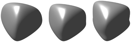
Figure 5. Meshes obtained by this new non-uniform scheme starting from the initial mesh (leftmost) in Figure 4 with $v_e^0=-2,-2.25,-2.5$ after 7 steps of subdivision.

Table 4 shows the Hausdorff distance between the initial mesh and the meshes after seven steps using this new non-uniform subdivision. From Table 4, we see the change of the Hausdorff distance with the change of $v_e^0$.

Table 4. The Hausdorff distance (hd) between the initial mesh and the meshes obtained after 7 steps using the new non-uniform scheme with different $v_e^0$.

$v_e^0$	−1	−1.3	−1.7	−2
hd	0.9215	0.9606	1.0105	1.0440

Example 3. 

Now we give two additional examples. Figure 6 and Figure 7 show the interpolation of the initial mesh (leftmost) with different values of $v_e^0$. The initial points in these two initial meshes have two kinds of valences: one with valence 4 and the other with valence 10. It can be seen from these two figures the interpolation of the initial meshes and the change of the shape of the limit surfaces with the change of $v_e^0$.

Figure 6. Meshes obtained by this non-uniform scheme starting from the initial mesh (leftmost) with $v_e^0=-0.1,-0.5,-1$ (left to right for the 3 meshes on the right) after 7 steps of subdivision.

Figure 7. Meshes obtained by this non-uniform scheme starting from the initial mesh (leftmost) with $v_e^0=-0.75,-1,-1.5$ (left to right for the 3 meshes on the right) after 7 steps of subdivision.

5. Conclusions

This paper presents a non-uniform, non-stationary Loop subdivision scheme developed through modification of a uniform, non-stationary variant. For this scheme, we have derived limit positions of initial vertices, generalizing existing theoretical results. These limit positions enable direct interpolation of initial meshes without requiring additional adjustment steps using finite steps of subdivision. Crucially, the interpolation process retains a free shape parameter that simultaneously controls the shape of the limit surface while maintaining interpolation. Although our examples demonstrate visually smooth surfaces, we have currently established only convergence properties. Future work will focus on rigorous smoothness analysis and exploring applications in domains such as computer animation.

References

- Loop, C. Smooth Subdivision Surfaces Based on Triangles. Master’s Thesis, University of Utah, Salt Lake City, UT, USA, 1987. [Google Scholar]
- Catmull, E.; Clark, J. Recursively generated B-spline surfaces on arbitrary topological meshes. Comput. Aided Geom. Des. 1978, 10, 350–355. [Google Scholar] [CrossRef]
- Andersson, L.-E.; Stewart, N.F. Introduction to the Mathematics of Subdivision Surfaces; SIAM: Philadelphia, PA, USA, 2010. [Google Scholar]
- Sun, L.; Ju, Z. Loop subdivision surface of progressive interpolation. Appl. Res. Comput. 2011, 28, 766–768. [Google Scholar]
- Zheng, J.; Cai, Y. Interpolation over arbitrary topology meshes using a two-phase subdivision scheme. IEEE Trans. Vis. Comput. Graph. 2006, 12, 301–310. [Google Scholar] [CrossRef] [PubMed]
- Deng, C.; Wang, G. Interpolating triangular meshes by Loop subdivision scheme. Sci. China Inf. Sci. 2010, 53, 1765–1773. [Google Scholar] [CrossRef][Green Version]
- Cheng, F.; Tao, F.; Lai, S.; Huang, C.; Wang, J.; Yong, J. Loop Subdivision Surface Based Progressive Interpolation. J. Comput. Sci. Technol. 2009, 24, 39–46. [Google Scholar] [CrossRef]
- Hamza, Y.F.; Hamza, M.F.; Rababah, A.; Rano, S.A. HSS-progressive interpolation for Loop and Catmull–Clark Subdivision Surfaces. Sci. Afr. 2024, 23, e02070. [Google Scholar] [CrossRef]
- Halstead, M.; Kass, M.; DeRose, T. Efficient, fair interpolation using Catmull-Clark surface. In Proceedings of the SIGGRAPH93’:Proceedings of the 20th Annual Conference on Computer Graphics and Interactive Techniques, Anaheim, CA, USA, 2–6 August 1993; pp. 35–44. [Google Scholar]
- Nasri, A. Polyhedral subdivision methods for free-form surfaces. ACM Trans. Graph. 1987, 6, 29–73. [Google Scholar] [CrossRef]
- Badoual, A.; Novara, P.; Romani, L.; Schmitter, D.; Unser, M. A non-stationary subdivision scheme for the construction of deformable models with sphere-like topology. Graph. Model. 2017, 94, 38–51. [Google Scholar] [CrossRef]
- Barrera, D.; Lamnii, A.; Nour, M.-Y.; Zidna, A. α-B-splines non-stationary subdivision schemes for grids of arbitrary topology design. Comput. Graph. 2022, 108, 34–48. [Google Scholar] [CrossRef]
- Lee, Y.; Yoon, J. Non-stationary subdivision schemes for surface interpolation based on exponential polynomials. Appl. Numer. Math. 2010, 60, 130–141. [Google Scholar] [CrossRef]
- Zhang, B.; Zheng, H.; Song, W. A non-stationary Catmull-Clark subdivision scheme with shape control. Graph. Model. 2019, 106, 101046. [Google Scholar] [CrossRef]
- Tan, J.; Sun, J.; Tong, G. A non-stationary binary three-point approximating subdivision scheme. Appl. Math. Comput. 2016, 276, 37–43. [Google Scholar] [CrossRef]
- Zhang, B.; Zhang, Y.; Zheng, H. A symmetric non-stationary Loop subdivision with applications in initial point interpolation. Symmetry 2024, 16, 379. [Google Scholar] [CrossRef]
- Ma, W.; Ma, X.; Tso, S.; Pan, Z. A direct approach for subdivision surface fitting from a dense triangle mesh. Comput.-Aided Des. 2004, 36, 525–536. [Google Scholar] [CrossRef]
- Dell’Accio, F.; Guessab, A.; Milovanović, G.V.; Nudo, F. Truncated Gegenbauer-Hermite weighted approach for the enrichment of the Crouzeix-Raviart finite element. BIT Numer. Math. 2025, 65, 24. [Google Scholar] [CrossRef]
- Fang, M.; Jeong, B.; Yoon, J. A family of non-uniform subdivision schemes with variable parameters for curve design. Appl. Math. Comput. 2017, 313, 1–11. [Google Scholar] [CrossRef]
- Beccari, C.; Casciola, G.; Romani, L. Polynomial-based non-uniform interpolatory subdivision with features control. J. Comput. Appl. Math. 2011, 235, 4754–4769. [Google Scholar] [CrossRef]
- Beccari, C.; Casiola, G.; Romani, L. Non-uniform non-tensor product local interpolatory subdivision surfaces. Comput. Aided Geom. Des. 2013, 30, 357–373. [Google Scholar] [CrossRef]
- Zhang, B.; Zheng, H.; Song, W.; Lin, Z.; Jie, Z. Interpolatory subdivision schemes with the optimal approximation order. Appl. Math. Comput. 2019, 347, 1–14. [Google Scholar] [CrossRef]
- Conti, C.; Dyn, N.; Manni, C.; Mazure, M. Convergence of univariate non-stationary subdivision schemes via asymptotic similarity. Comput. Aided Geom. Des. 2015, 37, 1–8. [Google Scholar] [CrossRef]
- Charina, M.; Conti, C.; Guglielmi, N.; Protasov, V. Regularity of non-stationary subdivision: A matrix approach. Numer. Math. 2017, 135, 639–678. [Google Scholar] [CrossRef]
- Novara, P.; Romani, L.; Yoon, J. Improving smoothness and accuracy of Modified Butterfly subdivision scheme. Appl. Math. Comput. 2016, 272, 64–79. [Google Scholar] [CrossRef]
- Beccari, C.; Casciola, G.; Romani, L. An interpolating 4-point C2 ternary non-stationary subdivision scheme with tension control. Comput. Aided Geom. Des. 2007, 24, 210–219. [Google Scholar] [CrossRef]
- Dyn, N.; Levin, D. Analysis of asymptotically equivalent binary subdivision schemes. J. Math. Anal. Appl. 1995, 193, 594–621. [Google Scholar] [CrossRef]
- Conti, C.; Donatelli, M.; Romani, L.; Novara, P. Convergence and normal continuity analysis of nonstationary subdivision schemes near extraordinary vertices and faces. Constr. Approx. 2019, 50, 457–496. [Google Scholar] [CrossRef]
Disclaimer/Publisher’s Note: The statements, opinions and data contained in all publications are solely those of the individual author(s) and contributor(s) and not of MDPI and/or the editor(s). MDPI and/or the editor(s) disclaim responsibility for any injury to people or property resulting from any ideas, methods, instructions or products referred to in the content. |
© 2025 by the authors. Licensee MDPI, Basel, Switzerland. This article is an open access article distributed under the terms and conditions of the Creative Commons Attribution (CC BY) license (https://creativecommons.org/licenses/by/4.0/).