Abstract
Outlier detection is pivotal in data mining and machine learning, as it focuses on discovering unusual behaviors that deviate substantially from the majority of data samples. Conventional approaches, however, often falter when dealing with complex data that are multimodal or sparse or that exhibit strong nonlinearity. To address these challenges, this paper introduces a novel outlier detection framework named Multimodal Granular Distance-based Outlier Detection (MGDOD), which leverages granular computing principles in conjunction with multimodal granulation techniques. Specifically, similarity measures and granulation methods are employed to generate granules from single-modal data, thereby reducing inconsistencies arising from different data modalities. These granules are then combined to form multimodal granular vectors, whose size, measurement, and operational rules are carefully defined. Building on this conceptual foundation, we propose two multimodal granular distance measures, which are formally axiomatized, and develop an associated outlier detection algorithm. Experimental evaluations on benchmark datasets from UCI, ODDS, and multimodal sources compare the proposed MGDOD method against established outlier detection techniques under various granulation parameters, distance metrics, and outlier conditions. The results confirm the effectiveness and robustness of MGDOD, demonstrating its superior performance in identifying anomalies across diverse and challenging data scenarios.
MSC:
68T37
1. Introduction
Outlier detection is a vital concern in data mining and machine learning, seeking to pinpoint unusual observations or patterns that stand apart from the bulk of a dataset. This field holds significant value in various applications, such as network security [], financial fraud detection [], product quality inspection [], and medical diagnosis []. Outlier detection techniques can generally be divided into several main categories, including statistical approaches [,,], distance-based strategies [,], density-focused methods [,,], model-based techniques [], and deep learning-based approaches [,,,].
Statistical methods include techniques such as Z-Score [], box plots [], and Grubbs’ Test []. These approaches are simple and interpretable but are often highly sensitive to noise and distributional assumptions, which limits their use in real-world high-dimensional or multimodal data. Distance-based methods leverage distances between data points for outlier detection, such as K-Nearest Neighbors (KNN) []. However, for high-dimensional datasets, distance-based approaches often face high computational complexity and the “curse of dimensionality.” Methods like DBSCAN [] and LOF [] detect anomalies by considering localized data concentration. While these methods perform well for data with varying densities, they are highly sensitive to parameters such as neighborhood size or density thresholds, which constrains robustness. For example, Sharma et al. [] applied LOF for detecting abnormal network routing, but performance degraded when parameters were poorly tuned. Wu et al. [] improved adaptability by using adaptive sliding windows, but such refinements increase computational burden and still lack guarantees of stability.
Model-based methods, such as One-Class SVM and Gaussian Mixture Models (GMMs), characterize the distribution of normal data. Lukashevich et al. [] demonstrated One-Class SVM’s advantage for high-dimensional and small-sample data, but scalability remains a challenge for large datasets. Ensemble methods such as Random Forests have also been adapted for anomaly detection, as in Hu et al. [], yet they require careful parameter tuning and may struggle with unbalanced data. In real-world applications such as financial fraud detection or industrial quality inspection, these models often suffer from high false alarm rates when encountering noise, missing modalities, or non-stationary distributions.
Traditional approaches thus struggle with nonlinear data and complex multimodal patterns, motivating the adoption of deep learning-based approaches. Recently, Wen et al. [] introduced a deep neural network framework for anomaly event detection, while Chen et al. [] surveyed graph-based anomaly detection. Advanced architectures such as adversarial networks [] and autoencoders [] have further improved representation learning for anomalies. However, deep learning methods typically demand large amounts of training data, are computationally expensive, and often lack interpretability. Moreover, they remain vulnerable to parameter sensitivity and can break down in scenarios such as real-time network monitoring or high-velocity sensor streams where scalability is critical.
Recently, with the emergence of large pretrained models, transformers and graph neural networks (GNNs) have been increasingly applied to anomaly detection. Transformer-based models show strong capacity in learning multimodal and spatio-temporal dependencies, achieving state-of-the-art results in video and time-series anomaly detection [,]. In parallel, GNN-based methods have been proposed to capture relational structures among multimodal features, enhancing robustness under complex dependencies []. Furthermore, self-supervised approaches have recently attracted attention, enabling anomaly detection without explicit labels and improving adaptability to unseen data distributions []. Despite their effectiveness, these architectures remain computationally demanding, are difficult to interpret, and often do not scale well to large, high-velocity multimodal streams. Another overlooked issue is that multimodal feature heterogeneity—differences in scale, distribution, and noise properties—can destabilize similarity measures, further reducing reliability.
In contrast, granular computing provides a complementary paradigm, offering flexible multigranular modeling with stronger interpretability. Polish scientist Pawlak’s early work on rough set theory and uncertainty laid the foundation for granular computing []. Skowron introduced the concept of “information granules” in 2001 [], emphasizing the partitioning of information into granular levels for better analysis. Building on fuzzy set theory, researchers such as Zadeh and Pedrycz extended granular computing for modeling uncertainty [,]. Information granularity, a key focus of granular computing, aims to organize and express information across multiple granular levels [,,]. Recent advances combine deep learning and granular computing for stronger representational capacity [,]. In anomaly detection, granular computing has shown promise in handling high-dimensional, heterogeneous, and multimodal data [,], where parameter sensitivity, scalability, and heterogeneity remain central challenges.
In summary, outlier detection remains an active research area, with ongoing efforts to handle uncertainty, multimodality, and large-scale data. Existing statistical, distance, density, and model-based methods suffer from parameter sensitivity and scalability issues, while deep learning methods often lack interpretability and robustness to heterogeneity. These limitations become more severe in real-world scenarios involving noisy, sparse, or high-velocity multimodal streams. The flexibility and multigranularity modeling capability of granular computing make it a powerful tool for addressing these challenges. Motivated by this, we propose a new method that defines multimodal granular vector representations and distances. Our preliminary experiments on multimodal and traditional datasets suggest competitive performance compared with representative techniques, highlighting the potential of granular computing as a promising direction for robust and interpretable outlier detection.
2. Multimodal Data Granulation
This section details the process of feature extraction from multimodal data, alongside the methodology for constructing granules and granular vectors.
Consider a multimodal dataset represented by . Here, is the collection of samples, and denotes the multimodal feature set. For each sample , the notation specifies the corresponding value of x under the particular feature m.
Multimodal data includes numeric, symbolic, audio, and image domains, among others. For two normalized numerical domain samples with dimensionality , their similarity measure is defined as
where denotes the order of the distance metric. In particular, corresponds to the Manhattan distance, and corresponds to the Euclidean distance.
Assuming that each feature has been normalized into the interval , it follows that , and thus . The measure is symmetric (), reaches its maximum value of 1 if and only if , and decreases monotonically as the distance between x and y increases.
For given symbolic domain samples , their similarity measures can be calculated using the following methods:
- (1)
- Hamming Similarity: , where are single characters.
- (2)
- Jaccard Coefficient: , where are sets of characters.
- (3)
- Cosine Similarity: , where are vectors.
For two segments of audio data, energy features, temporal features, and frequency features are extracted to form audio feature vectors x and y. The similarity between these two vectors is then evaluated using numerical domain methods. The extracted audio features span several categories, including energy-based metrics such as short-term energy and zero-crossing rate; temporal characteristics like root mean square (RMS); and frequency-based attributes that involve the Fourier transform, power spectrum density, and Mel-frequency cepstral coefficients (MFCCs). The specific formulas for feature extraction are as follows:
- (1)
- Energy Features
- A.
- Short-term Energy: , where denotes the signal amplitude, and N specifies the size of the window.
- B.
- Zero-Crossing Rate: , where N is the frame length. The factor is used for normalization to ensure that the ZCR values lie between 0 and 1.
- (2)
- Temporal Features
- A.
- Root Mean Square: , where N is the length of the signal.
- (3)
- Frequency Features
- A.
- Fourier Transform: . In this representation, corresponds to the signal in the frequency domain, whereas denotes its time-domain form.
- B.
- Power Spectrum Density: . Here, indicates how the signal’s power is distributed across frequencies.
- C.
- Mel-Frequency Cepstral Coefficients: , where F denotes the Fourier Transform.
Given image domain samples ImgA and ImgB, they are input into a pre-trained feature extraction backbone network (here, ResNet). The extracted feature vectors x and y are then used to calculate their similarity using numerical domain similarity measures. The feature extraction method based on the ResNet deep learning model is described as follows:
In our study, we rely on the pre-extracted acoustic, visual, and textual features provided by the CMU-MOSI dataset [], rather than extracting them ourselves.
Selecting a reference sample set , for a sample and a feature , granulation is performed on the reference samples, expressed as
where is the similarity measure between the sample x and the reference sample under modality m. Here, and represent feature vectors for the sample x and reference sample under the modality m, respectively.
These similarity values, , are initially computed as a set of scalar values quantifying the pairwise similarity between the sample x and each reference sample . However, for subsequent operations such as distance calculations, these similarity values are treated as vectors of fixed length p, meaning that each granule corresponds to a vector of length p derived from the reference sample set.
For a sample , granulation is performed on the multimodal features , constructing the multimodal granular vector , which is described as follows:
We employ concatenation to form multimodal granular vectors, as this preserves modality-specific granular information while allowing uniform distance computation across the combined representation. This approach avoids introducing strong assumptions about cross-modal correlations, which may otherwise bias the similarity measure. Although more sophisticated fusion schemes (e.g., attention-based or tensor factorization methods) could further exploit inter-modal dependencies, they often increase model complexity and reduce interpretability. Developing theoretically grounded fusion operators remains an important direction for future research.
3. A Multimodal Granular-Based Algorithm for Outlier Detection
3.1. Measures of Multimodal Granular Vectors
In the following, we present the fundamental operations related to granules and granular vectors, along with the approach for calculating distances between granular vectors.
Definition 1.
Given a granule , the magnitude of the granule is defined as
Definition 2.
Given two granules and , the operations of union, intersection, subtraction, and XOR are defined as follows:
Definition 3.
Let and represent two multimodal granular vectors. The operations of union, intersection, subtraction, and XOR between these vectors are defined as follows:
Definition 4.
Given two multimodal granular vectors and , their relative distance is defined as
In Equation (13), the similarity between two granules and is computed based on the ratio of their intersection to their union. To ensure numerical stability, we introduce a small constant in the denominator. This guarantees that the denominator never vanishes, even when both granules are zero vectors. Consequently, is always well-defined.
Definition 5.
Given two multimodal granular vectors and , the absolute distance between the two multimodal granular vectors is defined as
The normalization factor is introduced because each modality m contributes a granular vector of length p, and thus the total number of scalar similarity values across all modalities is . This ensures that is averaged over all entries of the multimodal granular representation and remains bounded within the unit interval.
It is straightforward to verify that where if and only if the two granular representations are identical, and when they are maximally different across all modalities.
3.2. Principles of Outlier Detection Based on Multimodal Granules
In the machine learning system, multimodal datasets are formed after feature extraction. The subsection introduces the definition and detection of outliers in multimodal datasets. The outlier degree of the object is computed using a defined formula, which is then used to identify outliers.
The distance between samples is measured using the granular vector distance metric. The outlier degree of a sample is then represented by the sum of its distances to all other samples. Samples with higher outlier degrees are considered outliers.
Definition 6.
Let be a multimodal dataset. For each sample , we define its anomaly degree through the Expected Outlier Factor (EOF). Formally,
where denotes the multimodal granular vector representation of sample x, and is the distance function defined on granular vectors.
In the current formulation, all modalities are equally weighted when computing the outlier degree. This design ensures fair treatment across heterogeneous modalities and avoids introducing additional hyperparameters. Nonetheless, in many real-world scenarios, certain modalities may be more informative than others. Future work will extend this framework to incorporate weighted or adaptive fusion strategies, for instance by learning modality-specific importance coefficients or leveraging attention-based mechanisms for multimodal fusion.
Intuitively, measures the average dissimilarity of sample with respect to all other samples in the dataset. Samples with larger values are considered more anomalous, as they are more distant from the majority of the data in the multimodal granular space.
3.3. Outlier Detection Algorithm Based on Multimodal Granules
The principle of multimodal granular outlier detection is explained in the previous subsection, and the multimodal granular outlier detection algorithm ide as shown in Algorithm 1.
In Algorithm 1, we first initialize the EOF score set E and the granular vector set to empty. In Steps 2–5, for each sample , its multimodal granular representation is constructed using Equation (3) and stored in the set . In Steps 6–14, the algorithm iterates over each granular vector and computes its pairwise distances to all other vectors—Equation (13). The average dissimilarity is then used to derive the Expected Outlier Factor (EOF) of each sample according to Equation (15). Finally, all EOF values are collected into the score set E, which constitutes the anomaly scores for the dataset.
| Algorithm 1 Multimodal granular outlier detection |
| Require: , where U denotes the sample set and M represents the multimodal feature set. Ensure: score set E
|
3.4. Time and Space Complexity Analysis
To evaluate the efficiency of the proposed method, we compare its computational complexity with a set of representative baseline algorithms. Let n denote the number of samples, m the feature dimensionality, k the number of nearest neighbors, b the number of histogram bins, t the number of base learners in ensemble methods, the subsample size, and i the number of clustering iterations. For the proposed granular approach, we denote p as the number of reference samples, resulting in a granular representation of length for each sample.
From Table 1, it can be observed that our method, similar to neighbor-based and granular methods such as KNN, LOF, SOD, and MFGAD, is dominated by pairwise sample comparisons, leading to quadratic complexity in n. However, while traditional granular methods such as MFGAD require pairwise comparisons in the original feature space of dimensionality m (resulting in ), our method first transforms each sample into a granular representation of length . Each inner loop iteration (Steps 8–10) requires computing one granular distance , whose complexity is O(mp). As a result, the pairwise comparison stage yields an overall complexity of , where the additional factor p reflects the reference set size and can be tuned to balance efficiency and accuracy.

Table 1.
Time complexity comparison of different methods.
In terms of memory usage, MFGAD maintains a similarity tensor of size , leading to space complexity, which scales quadratically with the dataset size n. In contrast, our method only requires storing a tensor of size , i.e., . Since in practical settings, the proposed method enjoys a significant space advantage, scaling linearly with n instead of quadratically, which makes it more suitable for large-scale datasets.
4. Experiments
To evaluate the effectiveness and robustness of the proposed anomaly detection method, we conduct extensive experiments on 16 diverse datasets, including both unimodal and multimodal data. These datasets cover a wide range of domains and characteristics, offering a comprehensive testbed for assessing generalization performance. For a fair and thorough comparison, we benchmark our method against 12 representative baseline algorithms, ranging from classical approaches to recent state-of-the-art techniques. The experimental results are organized into two parts. In the first part, we present ROC curve analysis to visualize performance trends, report AUC scores as a quantitative metric, and perform a statistical comparison using the Nemenyi test with Critical Difference (CD) diagrams to assess the overall significance across datasets. In the second part, we conduct parameter sensitivity analysis to examine the stability of our method under varying hyperparameter settings.
4.1. Datasets
The basic information of the datasets used in the experiments is summarized in Table 2. The datasets are collected from several publicly available repositories, including UCI1, ODDS2, and the CMU Multimodal Dataset Repository3. These datasets cover both unimodal and multimodal data types. For datasets containing categorical attributes, we encoded the categorical features into numerical values. If a dataset contains missing values, we performed imputation by filling missing numerical attributes with the mean value and categorical attributes with the mode. For datasets without predefined anomaly labels, we followed the common practice of treating the minority class as the anomaly class and the majority class as the normal class. Finally, all datasets were normalized using the standard normalization method to ensure fair comparisons among different methods.
Table 2.
Description of experimental data.
To ensure fair comparisons, we applied consistent data preprocessing across all evaluated algorithms. In particular, for the three high-dimensional multimodal datasets—Mosi, Sarcasm, and Sims—we employed an autoencoder-based dimensionality reduction technique. Each dataset was encoded using a specifically designed autoencoder architecture prior to anomaly detection, and the resulting latent representations were fed into both the proposed and baseline methods. For Mosi, the autoencoder comprised a single hidden layer with 16 units and a latent dimension of 10, trained using a learning rate of for 150 epochs with a batch size of 32. For Sarcasm, the network had one hidden layer with 64 units, a latent dimension of 10, and a learning rate of , and was trained for 40 epochs with a batch size of 16. For Sims, the autoencoder consisted of two hidden layers with 64 and 32 units respectively and a latent dimension of 10, and was trained with the same learning rate and epoch setting as Sarcasm. Given that these datasets originally exhibit near-balanced class distributions, one class was designated as the anomaly class, and a subset of its samples was randomly removed to achieve a controlled anomaly ratio suitable for unsupervised evaluation.
4.2. Comparison Methods
To evaluate the performance of the proposed method, we compare it with several mainstream anomaly detection algorithms, including distance-based methods such as K-Nearest Neighbors (KNN) []; density-based methods such as Local Outlier Factor (LOF) [], Histogram-based Outlier Score (HBOS) [], and Copula-Based Outlier Detection (COPOD) []; projection-based methods such as Subspace Outlier Detection (SOD) []; ensemble-based methods such as Isolation Forest (IForest) [], Lightweight Online Detector of Anomalies (LODA) [], and Sampling-based ensembles; clustering-based methods such as Cluster-Based Local Outlier Factor (CBLOF) []; and graph-based methods such as Instance-based Nearest Neighbor Ensembles (INNE) []. We also include ECOD [], a recently proposed explainable unsupervised anomaly detection method, and Multi-fuzzy Granules Anomaly Detection (MFGAD) [], which is based on fuzzy rough set theory and granular computing. These methods cover a broad range of classical and advanced anomaly detection paradigms.
To ensure fair and consistent evaluation, we perform parameter adjustment for all compared methods based on predefined ranges. For distance- and density-based methods such as KNN and LOF, the number of neighbors is adjusted from 5 to 15 with a step size of 1. Histogram-based methods such as HBOS and LODA are tuned by varying the number of histogram bins from 5 to 15, also with a step size of 1. Sampling-based ensemble methods are optimized by adjusting the subset proportion from 0.1 to 0.9 in increments of 0.1. For INNE, the number of reference samples is varied from 5 to 50 with a step size of 5. For MFGAD, the fuzziness threshold parameter is adjusted from 0.1 to 1.0 with a step size of 0.1. Our proposed method, MGDOD, also includes a tunable parameter controlling the number of reference samples, which is adjusted over the same range as in INNE: from 5 to 50, with a step size of 5.
For parameter-free methods such as ECOD and COPOD, as well as for CBLOF, SOD, and IForest—which are generally robust with their default settings—no manual adjustment is applied.
All hyperparameters are tuned exclusively on the training data to prevent any test data leakage. Except for the parameter sensitivity analysis, all reported results are obtained using 5-fold cross-validation to ensure the robustness of hyperparameter tuning and to mitigate the influence of data partitioning.
4.3. Evaluation Metrics
We selected widely used metrics in outlier detection to assess the performance of the algorithms. The receiver operating characteristic (ROC) curve [] is employed to illustrate the diagnostic ability of a binary classifier system, as its discrimination threshold varies. It plots the true positive rate (TPR) against the false positive rate (FPR) at different threshold settings, providing a comprehensive view of the trade-off between sensitivity and specificity. ROC curves are particularly useful in scenarios where the positive and negative class samples are relatively balanced, as they clearly show how well a model separates the two classes.
To quantitatively summarize the ROC curve, we use the area under the curve (AUC) as an evaluation metric. AUC measures the entire two-dimensional area underneath the ROC curve from (0,0) to (1,1). A larger AUC value indicates better overall detection performance, with a value of 1.0 representing a perfect classifier and 0.5 indicating a random guess.
In addition, we employ Friedman’s test [] with the Nemenyi [] post-hoc test to evaluate the statistical significance of the performance differences among multiple algorithms across multiple datasets. For each dataset, the algorithms are ranked based on their performance, and tied rankings are resolved by assigning the average of the tied ranks. After calculating the average ranking of each algorithm across all datasets, the Friedman test is applied to determine whether significant differences exist between the algorithms. The formula for calculating the Friedman test statistic is as follows:
where N represents the number of datasets, M denotes the number of algorithms, and refers to the average ranking of the i-th algorithm. Using the chi-square distribution table, we compare the calculated value to the critical value. If exceeds the critical value, it indicates a significant difference between at least some of the algorithms. The Nemenyi post-hoc test is then applied to identify which algorithm pairs exhibit statistically significant differences. The critical distance (CD) is computed as
where is the critical value from the Tukey distribution at a chosen significance level , M is the number of algorithms, and N is the number of datasets.
4.4. Experimental Results
As the first part of the experimental results, Figure 1 presents the ROC curves of all algorithms across 16 benchmark datasets. The proposed MGDOD, a granule-distance-based method, consistently demonstrates superior performance, with ROC curves closer to the top-left corner on most datasets. In particular, on ContraMC, Darwin, HighES, Mosi, Sarcasm, Sims, and WaveDG, MGDOD achieves significantly steeper curves compared to the baselines, reflecting its ability to detect anomalies early and with fewer false positives.
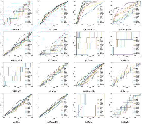
Figure 1.
ROC of all comparison methods on 16 experimental datasets.
In contrast, many competing methods produce flatter or overlapping curves, especially on datasets with complex structures or high-dimensional distributions. This highlights the advantage of modeling data characteristics through granule-level density estimation.
On datasets such as BreaCW, ChessN227, Derma, and Glass, the ROC curves of several algorithms intersect substantially, making visual comparison difficult. Therefore, we also report the Area Under the Curve (AUC) values to enable a more precise quantitative evaluation of detection performance.
To quantitatively assess the detection performance, we report the AUC values of all algorithms on the 16 benchmark datasets in Table 3. As shown, MGDOD achieves competitive or the highest AUC on the majority of datasets, highlighting its consistent superiority over existing methods in terms of median performance and overall rankings.
Table 3.
Experimental comparison results on ROC–AUC. The best performance for each dataset is indicated in bold.
In particular, MGDOD outperforms all baselines on 13 out of 16 datasets, such as Darwin (0.556), Sarcasm (0.742), Sims (0.558), Glass (0.871), and GongreVR (0.796), where other methods struggle to reach comparable accuracy. On several datasets such as Derma (0.991), Wine (0.892), and ChessN227 (0.873), although competing methods (e.g., LODA on Derma) also achieve strong performance, MGDOD still ranks among the top performers, indicating its strong generalization capability across both simple and complex data scenarios.
In contrast, some baseline methods such as Sampling, LODA, and CBLOF exhibit large performance fluctuations, particularly on high-dimensional or noisy datasets (e.g., Wine and Darwin), reflecting their limited robustness.
Notably, MGDOD achieves the highest average AUC score of 0.698, which is substantially higher than the second-best performer ECOD (0.567), followed by KNN (0.561) and COPOD (0.560). This considerable margin confirms the effectiveness of our granule-distance-based density modeling in capturing both global and local structures for anomaly detection.
These numerical results are consistent with the visual trends observed in the ROC curves and provide solid evidence of the proposed method’s accuracy and reliability.
To examine whether the performance differences observed in AUC values are statistically significant, we perform a non-parametric Friedman test followed by a Nemenyi post-hoc test. The Friedman test evaluates the null hypothesis that all algorithms perform equivalently across datasets. The test was applied to the AUC scores of 13 algorithms over 16 datasets, with average ranks computed based on per-dataset rankings.
The Friedman statistic yielded a value of , corresponding to a p-value of . Since exceeds the critical value of 1.806 at the significance level, the null hypothesis is rejected, confirming the existence of statistically significant differences in performance among the algorithms.
Following this, we conducted the Nemenyi post-hoc test to identify which pairs of algorithms differ significantly. With , the critical value is 3.314, leading to a computed critical difference (CD) of 4.561. As shown in Figure 2, MGDOD achieves the best average rank and is clearly separated from the majority of baseline methods, indicating its statistically superior performance.
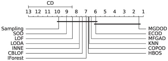
Figure 2.
Nemenyi test diagram for AUC results.
These results not only support the observations drawn from the ROC curves and AUC metrics, but also validate that MGDOD’s improvements are consistent and significant across diverse datasets.
4.5. Parameter Sensitivity Analyses
To evaluate the robustness of the proposed method (MGDOD) with respect to the number of reference samples, we conduct a sensitivity analysis across multiple datasets. In this experiment, the number of reference samples is systematically varied, and the corresponding AUC scores are recorded to assess the algorithm’s stability.
As shown in Figure 3, the influence of this parameter differs across datasets. On ContraMC and Mosi, the AUC values tend to decrease as the number of reference samples increases, before reaching a stable plateau. This suggests that an overly large reference set may blur the distinction between normal and anomalous granules by flattening the granule distance contrast.
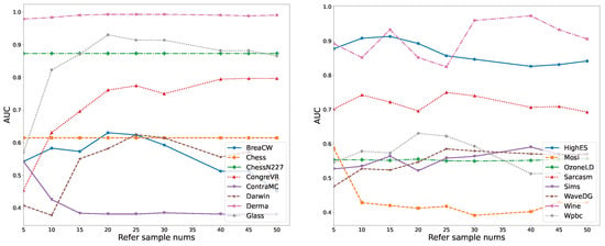
Figure 3.
AUC variation with Refer sample nums parameter.
In contrast, for datasets such as GongreVR and Derma, the AUC scores increase steadily with more reference samples. In these cases, expanding the reference set enhances the granule comparison process, leading to more accurate anomaly estimations.
Interestingly, the AUC values on Chess, ChessN227, and OzoneLD remain nearly unchanged regardless of the number of reference samples, implying that the underlying granule structure is inherently well-separated and less sensitive to parameter tuning.
For the other datasets, we observe that AUC performance often peaks when the number of reference samples falls within a moderate range, reflecting a trade-off between granule representation and redundancy. Too few reference samples may underrepresent the granule landscape, while too many may introduce noise or dilute anomaly signals.
In summary, the results in Figure 3 demonstrate that MGDOD maintains stable and reliable performance across most datasets, and achieves optimal results when the reference sample size is set within a reasonable range.
5. Conclusions
This paper introduces a novel Multimodal Granular Distance-based Outlier Detection (MGDOD) framework that effectively addresses the challenges of detecting anomalies in complex multimodal, sparse, and nonlinear data. The approach leverages granular computing principles to construct granular representations from diverse data modalities and establishes rigorous mathematical definitions for granular operations with two novel distance measures. The MGDOD algorithm employs the Expected Outlier Factor (EOF) to measure sample dissimilarity, providing a principled method for anomaly identification. Comprehensive experiments on 16 benchmark datasets demonstrate superior performance, with MGDOD achieving the highest average AUC score of 0.698 and statistical significance confirmed through Friedman test (). The method maintains space complexity, providing significant scalability advantages while offering enhanced interpretability and flexibility across various data modalities. While the current approach employs equal weighting for all modalities, future work should explore adaptive fusion strategies and semi-supervised variants. The consistent improvements across diverse datasets, combined with computational efficiency and parameter stability, demonstrate that granular distance-based approaches represent a promising direction for robust and interpretable outlier detection in complex multimodal environments.
Author Contributions
Conceptualization, T.H. and S.Z.; methodology, S.Z.; software, S.Z.; validation, T.H. and S.Z.; formal analysis, S.Z.; investigation, T.H.; resources, H.L.; data curation, J.L.; writing—original draft preparation, T.H. and S.Z.; writing—review and editing, Y.Z. and Y.C.; visualization, S.Z.; supervision, Y.C.; project administration, S.Z.; funding acquisition, Y.C. All authors have read and agreed to the published version of the manuscript.
Funding
The authors would like to thank all reviewers for their valuable comments. This work was supported by the Fujian Provincial Natural Science Foundation of China, grant number 2024J011192 and the Natural Science Foundation of Xiamen, China, grant number 3502Z202473069.
Data Availability Statement
The source code and configuration files supporting this study are openly available in the MGDOD repository at https://github.com/Fa-Xiao/MGDOD (accessed on 25 July 2025). All datasets used in this study are publicly available and can be downloaded from the original sources as cited in Section 4.1 ‘Datasets’.
Conflicts of Interest
Authors Tiancai Huang, Hao Luo and Jinsong Lyu were employed by Xiamen Taqu Information Technology Co., Ltd. The remaining authors declare that the research was conducted in the absence of any commercial or financial relationships that could be construed as a potential conflict of interest.
References
- Hong, J.; Liu, C.C.; Govindarasu, M. Integrated anomaly detection for cyber security of the substations. IEEE Trans. Smart Grid 2014, 5, 1643–1653. [Google Scholar] [CrossRef]
- Loperfido, N. Kurtosis-based projection pursuit for outlier detection in financial time series. Eur. J. Financ. 2020, 26, 142–164. [Google Scholar] [CrossRef]
- Lyu, J.; Manoochehri, S. Online convolutional neural network-based anomaly detection and quality control for fused filament fabrication process. Virtual Phys. Prototyp. 2021, 16, 160–177. [Google Scholar] [CrossRef]
- Gao, H.; Zhou, L.; Kim, J.Y.; Li, Y.; Huang, W. Applying probabilistic model checking to the behavior guidance and abnormality detection for A-MCI patients under wireless sensor network. ACM Trans. Sens. Netw. 2023, 19, 1–24. [Google Scholar] [CrossRef]
- Yaro, A.S.; Maly, F.; Prazak, P. Outlier Detection in Time-Series Receive Signal Strength Observation Using Z-Score Method with S n Scale Estimator for Indoor Localization. Appl. Sci. 2023, 13, 3900. [Google Scholar] [CrossRef]
- Dovoedo, Y.; Chakraborti, S. Boxplot-based outlier detection for the location-scale family. Commun. Stat. Simul. Comput. 2015, 44, 1492–1513. [Google Scholar] [CrossRef]
- Grubbs, F.E. Procedures for detecting outlying observations in samples. Technometrics 1969, 11, 1–21. [Google Scholar] [CrossRef]
- Ying, S.; Wang, B.; Wang, L.; Li, Q.; Zhao, Y.; Shang, J.; Huang, H.; Cheng, G.; Yang, Z.; Geng, J. An improved KNN-based efficient log anomaly detection method with automatically labeled samples. ACM Trans. Knowl. Discov. Data (TKDD) 2021, 15, 1–22. [Google Scholar] [CrossRef]
- Hu, M.; Wang, K.; Li, H.; Chen, L. Random forest and anomaly detection of fuzzy tree nodes. Nanjing Univ. Nat. Sci. 2018, 54, 1141–1151. [Google Scholar]
- Aslan, M.E.; Onut, S. Detection of outliers and extreme events of ground level particulate matter using DBSCAN algorithm with local parameters. Water Air Soil Pollut. 2022, 233, 203. [Google Scholar] [CrossRef]
- Sharma, T.; Mohapatra, A.K.; Tomar, G. A novel SVM and LOF-based outlier detection routing algorithm for improving the stability period and overall network lifetime of WSN. Int. J. Nanotechnol. 2023, 20, 759–789. [Google Scholar] [CrossRef]
- Wu, Q.; Zhang, X.; Zhao, B. A novel adaptive kernel-guided multi-condition abnormal data detection method. Measurement 2023, 206, 112257. [Google Scholar] [CrossRef]
- Lukashevich, H.; Dittmar, C. Improving GMM classifiers by preliminary one-class SVM outlier detection: Application to automatic music mood estimation. In Classification as a Tool for Research, Proceedings of the 11th IFCS Biennial Conference and 33rd Annual Conference of the Gesellschaft für Klassifikation eV, Dresden, 13–18 March 2009; Springer: Berlin/Heidelberg, Germany, 2010; pp. 775–782. [Google Scholar]
- Wen, J.; Wang, H.; Deng, J.; Deng, P. Abnormal Event Detection Based on Deep Learning. Chin. J. Electron. 2020, 48, 308–313. [Google Scholar]
- Chen, B.; Li, J.; Lu, X.; Sha, C.; Wang, X.; Zhang, J. Survey of Deep Learning Based Graph Anomaly Detection Methods. J. Comput. Res. Dev. 2021, 58, 1436–1455. [Google Scholar]
- Chen, Z.; Duan, J.; Kang, L.; Qiu, G. Supervised anomaly detection via conditional generative adversarial network and ensemble active learning. IEEE Trans. Pattern Anal. Mach. Intell. 2022, 45, 7781–7798. [Google Scholar] [CrossRef]
- Wang, Y.; Zhou, Y.; Ma, J. A locational false data injection attack detection method in smart grid based on adversarial variational autoencoders. Appl. Soft Comput. 2024, 151, 111169. [Google Scholar] [CrossRef]
- Dilek, E.; Dener, M. An overview of transformers for video anomaly detection. Neural Comput. Appl. 2025, 37, 17825–17857. [Google Scholar] [CrossRef]
- Kang, H.; Kang, P. Transformer-based multivariate time series anomaly detection using inter-variable attention mechanism. Knowl. Based Syst. 2024, 290, 111507. [Google Scholar] [CrossRef]
- Zheng, X.; Wu, B.; Zhang, A.X.; Li, W. Improving Robustness of GNN-based Anomaly Detection by Graph Adversarial Training. In Proceedings of the 2024 Joint International Conference on Computational Linguistics, Language Resources and Evaluation (LREC-COLING 2024), ELRA and ICCL, Torino, Italia, 20–25 May 2024; pp. 8902–8912. [Google Scholar]
- Hojjati, H.; Ho, T.K.K.; Armanfard, N. Self-supervised anomaly detection in computer vision and beyond: A survey and outlook. Neural Netw. 2024, 172, 106106. [Google Scholar] [CrossRef]
- Pawlak, Z. Rough sets. Int. J. Comput. Inf. Sci. 1982, 11, 341–356. [Google Scholar] [CrossRef]
- Skowron, A. Toward intelligent systems: Calculi of information granules. In New Frontiers in Artificial Intelligence, Proceedings of the Joint JSAI 2001 Workshop Post-Proceedings; Springer: Berlin/Heidelberg, Germany, 2001; pp. 251–260. [Google Scholar]
- Zadeh, L.A. Toward a theory of fuzzy information granulation and its centrality in human reasoning and fuzzy logic. Fuzzy Sets Syst. 1997, 90, 111–127. [Google Scholar] [CrossRef]
- Lu, W.; Pedrycz, W.; Liu, X.; Yang, J.; Li, P. The modeling of time series based on fuzzy information granules. Expert Syst. Appl. 2014, 41, 3799–3808. [Google Scholar] [CrossRef]
- Qian, Y.; Liang, J.; Wei-zhi, Z.W.; Dang, C. Information granularity in fuzzy binary GrC model. IEEE Trans. Fuzzy Syst. 2010, 19, 253–264. [Google Scholar] [CrossRef]
- Miao, D.; XU, F.; Yao, Y.; Wei, L. Set-Theoretic Formulation of Granular Computing. Chin. J. Comput. 2012, 35, 2351–2363. [Google Scholar] [CrossRef]
- Chen, Y.; Qin, N.; Li, W.; Xu, F. Granule structures, distances and measures in neighborhood systems. Knowl. Based Syst. 2019, 165, 268–281. [Google Scholar] [CrossRef]
- Chen, Y.; Zhang, X.; Zhuang, Y.; Yao, B.; Lin, B. Granular neural networks with a reference frame. Knowl. Based Syst. 2023, 260, 110147. [Google Scholar] [CrossRef]
- Song, M.; Jing, Y.; Pedrycz, W. Granular neural networks: A study of optimizing allocation of information granularity in input space. Appl. Soft Comput. 2019, 77, 67–75. [Google Scholar] [CrossRef]
- Zhu, X.; Pedrycz, W.; Li, Z. Granular models and granular outliers. IEEE Trans. Fuzzy Syst. 2018, 26, 3835–3846. [Google Scholar] [CrossRef]
- Yuan, Z.; Chen, H.; Luo, C.; Peng, D. MFGAD: Multi-fuzzy granules anomaly detection. Inf. Fusion 2023, 95, 17–25. [Google Scholar] [CrossRef]
- Zadeh, A.; Zellers, R.; Pincus, E.; Morency, L.P. Mosi: Multimodal corpus of sentiment intensity and subjectivity analysis in online opinion videos. arXiv 2016, arXiv:1606.06259. [Google Scholar] [CrossRef]
- Goldstein, M.; Dengel, A. Histogram-based outlier score (hbos): A fast unsupervised anomaly detection algorithm. In Proceedings of the KI-2012: Poster and Demo Track, Saarbrucken, Germany, 24–27 September 2012; pp. 59–63. [Google Scholar]
- Li, Z.; Zhao, Y.; Botta, N.; Ionescu, C.; Hu, X. Copod: Copula-based outlier detection. In Proceedings of the 2020 IEEE International Conference on Data Mining (ICDM), Sorrento, Italy, 17–20 November 2020; IEEE: New York, NY, USA, 2020; pp. 1118–1123. [Google Scholar]
- Kriegel, H.P.; Kröger, P.; Schubert, E.; Zimek, A. Outlier detection in axis-parallel subspaces of high dimensional data. In Advances in Knowledge Discovery and Data Mining, Proceedings of the 13th Pacific-Asia Conference, PAKDD 2009, Bangkok, Thailand, 27–30 April 2009; Proceedings 13; Springer: Berlin/Heidelberg, Germany, 2009; pp. 831–838. [Google Scholar]
- Liu, F.T.; Ting, K.M.; Zhou, Z.H. Isolation forest. In Proceedings of the 2008 Eighth Ieee International Conference on Data Mining, Pisa, Italy, 15–19 December 2008; IEEE: New York, NY, USA, 2008; pp. 413–422. [Google Scholar]
- Pevnỳ, T. Loda: Lightweight on-line detector of anomalies. Mach. Learn. 2016, 102, 275–304. [Google Scholar] [CrossRef]
- He, Z.; Xu, X.; Deng, S. Discovering cluster-based local outliers. Pattern Recognit. Lett. 2003, 24, 1641–1650. [Google Scholar] [CrossRef]
- Bandaragoda, T.R.; Ting, K.M.; Albrecht, D.; Liu, F.T.; Zhu, Y.; Wells, J.R. Isolation-based anomaly detection using nearest-neighbor ensembles. Comput. Intell. 2018, 34, 968–998. [Google Scholar] [CrossRef]
- Li, Z.; Zhao, Y.; Hu, X.; Botta, N.; Ionescu, C.; Chen, G.H. Ecod: Unsupervised outlier detection using empirical cumulative distribution functions. IEEE Trans. Knowl. Data Eng. 2022, 35, 12181–12193. [Google Scholar] [CrossRef]
- Fawcett, T. An introduction to ROC analysis. Pattern Recognit. Lett. 2006, 27, 861–874. [Google Scholar] [CrossRef]
- Friedman, M. A comparison of alternative tests of significance for the problem of m rankings. Ann. Math. Stat. 1940, 11, 86–92. [Google Scholar] [CrossRef]
- Douglas, C.E.; Michael, F.A. On distribution-free multiple comparisons in the one-way analysis of variance. Commun. Stat. Theory Methods 1991, 20, 127–139. [Google Scholar] [CrossRef]
Disclaimer/Publisher’s Note: The statements, opinions and data contained in all publications are solely those of the individual author(s) and contributor(s) and not of MDPI and/or the editor(s). MDPI and/or the editor(s) disclaim responsibility for any injury to people or property resulting from any ideas, methods, instructions or products referred to in the content. |
© 2025 by the authors. Licensee MDPI, Basel, Switzerland. This article is an open access article distributed under the terms and conditions of the Creative Commons Attribution (CC BY) license (https://creativecommons.org/licenses/by/4.0/).