Computation of the Approximate Symmetric Chordal Metric for Complex Numbers

Abstract

The basic theoretical properties of the approximate symmetric chordal metric (ASCM) for two real or complex numbers are studied, and reliable, accurate, and efficient algorithms are proposed for its computation. ASCM is defined as the minimum between the moduli of the differences of the two numbers and of their reciprocals. It differs from the chordal metric by including the modulus of the difference of the numbers. ASCM is not a true mathematical distance, but is a useful replacement for a distance in some applications. For instance, sensitivity analysis or block diagonalization of matrix pencils benefit from a measure of closeness of eigenvalues and also of their reciprocals; ASCM is ideal for this purpose. The proposed algorithms can be easily implemented on various architectures and compilers. Extensive numerical tests were performed to assess the performance of the associated implementation. The results were compared to those obtained in MATLAB, but with appropriate modifications for numbers very close to the bounds of the range of representable values, where the usual formulas give wrong results.

1. Introduction

The approximate symmetric chordal metric for two real or complex numbers is defined by

$$d(a_1,a_2):=\min \left(\right|a_1-a_2|,|1/a_1-1/a_2\left|\right)=:\min (d_1,d_2).$$

(1)

It differs from the Euclidean distance by also considering the absolute difference of the reciprocals of the given numbers. It is not a true mathematical distance, but can be used instead of a distance in some applications.

The approximate symmetric chordal metric in (1) measures the closeness of two numbers. In mathematics, a measure is a function that assigns a non-negative number to certain subsets of a set. Using pairwise distances (1) of a set of numbers, it is possible to build subsets (clusters) and a measure of their closeness. Measures are used in various fields, including analysis, probability theory, and geometry, as well as in sophisticated investigations and computational techniques.

There are quite a number of references on the chordal metric, but no references to the approximate symmetric chordal metric could be found. Klamkin and Meir [1] have shown that the chordal metric on a normed linear space, defined as $d(x,y)=\parallel x-y\parallel /\parallel x\parallel /\parallel y\parallel$, x, $y\ne 0$, satisfies the triangle inequality. Let $S^2\subset {\mathbb{R}}^3$ be the Riemann sphere with diameter 1 and center $(0,0,1/2)$. With z, $w\in \mathbb{C}$, $d(z,w)=|z-w|$ Euclidean metric in $\mathbb{C}$, the chordal metric of $S^2$ is [2,3,4]

$$\underline{d}(z,w):=d(\chi \left(z\right),\chi \left(w\right))={\displaystyle \frac{|z-w|}{\sqrt{1+{\left|z\right|}^2}\sqrt{1+{\left|w\right|}^2}}},$$

(2)

where $\chi :\mathbb{C}\to S^2\setminus N:z\mapsto {(\Re \left(z\right),\Im \left(z\right),|z|}^2{)/(1+\left|z\right|}^2)$ is the stereographic projection, $\mathbb{C}$ is the complex plane, and N is the north pole of $S^2$. Clearly, $d\left(\chi \right(z),\chi (w\left)\right)=0\iff d(z,w)=0$ and $\underline{d}(z,w)=\underline{d}(1/z,1/w)$. If $z\to \infty$, then $\chi \left(z\right)\to N$. This way, $\chi$ maps the extended complex plane $\overline{\mathbb{C}}=\mathbb{C}\cup \{\infty \}$ to $S^2$. The chordal metric is indeed a distance, since $d\left(\chi \right(z),\chi (w\left)\right)$ satisfies triangle inequality. If $w\to \infty$, then $\underline{d}(z,w)\to 1/\sqrt{1+{\left|z\right|}^2}$, and if $z\to \infty$ too, then $\underline{d}(z,w)\to 0$. If a sphere with unit radius and center in the origin is used, the right hand side in (2) is multiplied by 2 [3,5].

Several authors present theoretical results and various applications of the chordal metric. Rainio and Vuorinen [4] use (2) to identify cases where the distortion caused by symmetrization of a quadruple of objects, mapped by a Möbius transformation, can be measured in terms of its Lipschitz constant in the Euclidean or the chordal metric. Álvarez-Tuñón et al. [6] investigate various pose representations in visual odometry networks, and show that the chordal distance between two rotations ensures faster convergence of the parameters than distances measured by Euler angles or quaternions. Xu et al. [7] provide sharper bounds of the chordal metric between generalized singular values of Grassmann matrix pairs. Sun [8] shows that the generalized singular values of $[A;B]$, with $\mathrm{rank}\left(\right[A;B\left]\right)<n$, and A and B complex $m\times n$ and $p\times n$, are insensitive to strong perturbations in the elements of A and B, if the chordal metric is used to describe such perturbations. Sasane [2] defines an abstract chordal metric on linear control systems described by transfer functions and shows that strong stabilizability is a robust property in this metric. A refinement of this metric for stable transfer functions is introduced in [9].

A possible application of the approximate symmetric chordal metric is ordering the (generalized) eigenvalues of a matrix (pencil), according to their pairwise distances measured using (1). This is important in numerical linear algebra, control theory, and other domains. For instance, it is essential for computing invariant or deflating subspaces of matrices or matrix pencils, respectively, or of their block-diagonal form [10]. The available algorithms for finding this form use non-unitary transformation matrices with a controlled numerical condition, but they can be inefficient for a matrix (pencil) with dense clusters of eigenvalues. Since the numerical condition is related to the sensitivity of the spectrum associated to the current block (pair) that should be split, a clever strategy for ordering the eigenvalues may increase the efficiency. The sensitivity of eigenvalue problems is investigated in [11,12,13,14,15,16]. Efficient and reliable implementations of the theoretical results are available in the LAPACK package [17] and in recent releases of interactive environments like MATLAB [18] or Mathematica [19]. The applications mentioned in this paragraph do not need the triangle inequality, but it is important that close eigenvalues be included in the same cluster. With (1), an eigenvalue $a_2$ will be added to a cluster containing a value $a_1$ if either $d_1$ or $d_2$ is smaller than a given threshold. If $a_1\ne 0$, $a_2\ne 0$, $d_2=|a_1-a_2|/|a_1|/|a_2|$ coincides to the chordal metric in [1], and it is an approximation of the value given by (2). So, an approach based on the chordal metric will choose $d_2$ or its approximation, even if $d_1<d_2$. If $a_1$ and $a_2$ are eigenvalues for a matrix pencil defined by $A-\lambda B$, then $1/a_1$ and $1/a_2$ are eigenvalues of the matrix pencil $B-\mu A$. Since A and B have a symmetric role, it is reasonable to consider the closeness of eigenvalues for both $A-\lambda B$ and $B-\mu A$.

The idea of decoupling a dynamical system to simpler subsystems, preserving the essential dynamics, has been recently extended to certain nonlinear systems, mainly described by ordinary differential equations (ODE) or difference equations. A so-called normal form is obtained using a near-identity transformation of coordinates, preserving the essential system behavior near an equilibrium point. Higher-order Taylor expansion of the system model can capture the major nonlinear effects. An application of the normal form theory to power systems described by differential algebraic equations (DAE) is studied in [20]. The new, structure-preserving method allows direct application of the theory to the DAE system.

A main contribution of the paper is the systematic presentation of the properties of the approximate symmetric chordal metric and of reliable, accurate and efficient algorithms for its computation. A factored representation of the modulus of complex numbers is introduced, which allows obtaining very accurate results for the entire range of the floating point system. Two different approaches to evaluate $d_2$ are described. The most efficient approach needs only the moduli of the two numbers and of their difference, but it cannot be used if that difference is not in the range of representable numbers. The proposed algorithms were implemented in Fortran and exhaustively tested in MATLAB.

The rest of the paper is organized as follows. Section 2 summarizes the notation and the main issues concerning the floating point system of computers, needed in the sequel. Section 3 investigates the properties of the approximate symmetric chordal metric, while Section 4 presents reliable, accurate, and efficient algorithms for its computation. Section 5 discusses the numerical results obtained using a careful implementation of these algorithms. Section 6 summarizes the conclusions.

2. Preliminaries

For technical convenience, $\overline{\mathbb{R}}$ will denote the real numbers field $\mathbb{R}$ extended by the ∞ and $-\infty$ symbols, and similarly for $\overline{\mathbb{C}}$. A complex number $a=\alpha +\beta 𝚤$, with $\alpha ,\beta \in \overline{\mathbb{R}}$, is infinite if $\alpha =\pm \infty$ and/or $\beta =\pm \infty$; otherwise, a is finite. Let $a_1={\alpha }_1+{\beta }_1𝚤$, $a_2={\alpha }_2+{\beta }_2𝚤$ be two finite complex numbers. For performing computations with/on $a_1$ and $a_2$, it should be assumed that ${\alpha }_i$ and ${\beta }_i$, $i=1,2$, are in the range of the computer floating point system, that is, $a_1$ and $a_2$ are (approximately) representable by their real and imaginary parts. Hence, $\left|{\alpha }_i\right|,\left|{\beta }_i\right|\le K$, $i=1,2$, where K is the maximum representable number,

$$K:=b^{e_M}(1-ϵ),$$

(3)

with b the base of the numeral system, $e_M$ the maximum exponent, and $ϵ$ the relative machine precision. In a common binary double precision floating point system, $b=2$, $e_M=1024$, $ϵ=2^{1-t}$ (or $ϵ=2^{-t}$ for machines with proper rounding), and $t=53$ is the number of base digits in the mantissa. The number $\epsilon =bϵ$ is called precision. Representable real numbers in a digital computer are rational approximations of values in the range $\left[-K,K\right]$. An overflow is generated if an arithmetic operation would produce a result outside this range. Compilers and interactive environments may represent such a result as ±Infinity or ±Inf, and if this happens in a sequence of computations, the final result might be completely wrong. Hence, overflows should be avoided. Very small (in magnitude) numbers may also be not representable, and if this so-called underflow happens after an arithmetic operation, the result is set to zero. The underflow threshold is defined by $k=b^{e_m-1}$, where $e_m$ is the minimum exponent before underflow. For the machine considered above, $e_m=-1021$. Many computer systems allow for gradual underflow, i.e., they may also use numbers less than k, in the range $\left[\epsilon k,k\right)$. Algorithms for discovering the properties of the floating point arithmetic, as in [21,22], are implemented, e.g., in the SLAMCH and DLAMCH routines of the LAPACK package [17], for single and double precision computations, respectively.

The assumption that $\left|{\alpha }_i\right|,\left|{\beta }_i\right|\le K$, does not imply that $\left|a_i\right|\le K$. If $\left|{\alpha }_1\right|=K$ and $\left|{\beta }_1\right|=K$, then $\left|a_1\right|=K\sqrt{2}$, which is not representable. The specific case of our problem allows working with a factored form of $\left|a_1\right|$ and $\left|a_2\right|$.

3. Basic Properties of the Approximate Symmetric Chordal Metric

In some applications using the (approximate symmetric) chordal metric, $a_1$ and/or $a_2$ or the terms in (1) may not be numbers, but 0/0 or $\infty -\infty$. For instance, some eigenvalues can be infinite even for regular matrix pencils. If $a_1=a_2=\infty$ in (1), for $a_1$, $a_2\in \overline{\mathbb{R}}$, then $d_1$ is $\infty -\infty$. A Not-a-Number entity is represented by NaN in compilers and interactive environments, and  special computer rules are used for mathematical operations. Specifically, in the paper context, the basic rules are $\left|\mathtt{NaN}\right|=\mathtt{NaN},\min (\mathtt{NaN},a)=a,max(\mathtt{NaN},a)=a,a\in \overline{\mathbb{C}}.$ The properties below follow directly from (1) and these rules.

• Basic properties of d in (1). Let a, $a_1,a_2\in \overline{\mathbb{C}}$. Then, with (1)

  (i)

$d(a_1,a_2)=d(a_2,a_1)$;

 (ii)

$d(a,0)=\left|a\right|$;

(iii)

$d(a,a)=0$;

(iv)

$d(a_1,a_2)=0\iff a_1=a_2$;

 (v)

$d(a_1,a_2)=1/\left|a_1\right|$, if $a_2$ is infinite;

(vi)

$d(a_1,a_2)>0$ if $a_1\ne a_2$ and $a_1$ or $a_2$, or both, are finite.

Remark 1.

The three properties of a distance or metric, namely, symmetry (i), identity (iv), and non-negativity (iii) and (vi), are satisfied by $d(a_1,a_2)$. But it is easy to verify that the fourth needed property, the triangle inequality, does not hold for (1), in general. Consequently, $d(a_1,a_2)$ is not a distance or metric function. Moreover, $d(s{a}_1,s{a}_2)$ may differ from $\left|s\right|d(a_1,a_2)$, with $a_1,a_2,s\in \mathbb{C}$. Such property holds for $|a_1-a_2|$ and for $|1/a_1-1/a_2|$, but not necessarily for their minimum.

Definition 1.

(Factored representation of the absolute value of a complex number a) Let $a=\alpha +\beta 𝚤\in \mathbb{C}$ with $\left|\alpha \right|\le K$ and $\left|\beta \right|\le K$. Let $M:=max\left(\right|\alpha |,|\beta \left|\right)$, $m=\min \left(\right|\alpha |,|\beta \left|\right)$, and $\delta =\sqrt{1+{(m/M)}^2}$. Then, $\left|a\right|=M\delta$ is called the factored representationof $\left|a\right|$.

From Definition 1, it follows that $\delta \in \left[1,\sqrt{2}\right]$, since $\delta =1$ if $m=0$, $\delta =\sqrt{2}$ if $m=M$, and $\delta \in \left(1,\sqrt{2}\right)$ for $m/M\in \left(0,1\right)$. Factored representation is useful when M is very close or coincides to K. Then, $M\delta$ could exceed K, and $\left|\alpha \right|$ cannot be computed. Still, its factors can be used for finding the approximate symmetric chordal metric.

4. Algorithms for Computing the Approximate Symmetric Chordal Metric

A mathematical-style pseudocode is used for each algorithm. A MATLAB-style function construct, with possibly optional arguments, is adopted for calling lower level algorithms. See Remark 3 in Section 4.2. The symbols ∧, ∨, and ¬, appearing in the algorithms and their description, are the binary logical operators AND, OR, and NOT, respectively. Moreover, ${\overline{\mathbb{C}}}_r$ and ${\overline{\mathbb{R}}}_r$ denote the sets of complex and real representable numbers, respectively. However, the algorithms below will also work correctly for $a_1$ and/or $a_2$ set to ±Infinity or ±Infinity±Infinity𝚤, if the IEEE arithmetic is available on the computer. Although the computational problem for approximate symmetric chordal metric is mathematically very simple, a reliable, accurate, and efficient implementation needs a thorough analysis. These desirable properties are supported by careful consideration of all possible special cases and lower level algorithms. Efficiency can be measured by an estimate of the number of floating point operations, or flops, which have been used especially for numerical linear algebra algorithms [11,23]. There are several definitions for a flop, but counting each arithmetic operation is suitable in the paper context.

4.1. Main Algorithm

This subsection presents the main algorithm, chordal (Algorithm 1). The lower level algorithms are introduced in the next subsections.

Algorithm 1  chordal computes ASCM for two complex numbers

Require: $a_1,a_2\in {\overline{\mathbb{C}}}_r$, $a_i={\alpha }_i+{\beta }_i𝚤$, K in (3), $\epsilon$. Ensure: $d:=d(a_1,a_2)=\min \left(\right|a_1-a_2|,|1/a_1-1/a_2\left|\right)$     $M_i=max\left(\right|{\alpha }_i|,|{\beta }_i\left|\right),i=1,2,M=max(M_1,M_2)$     if $M=0$ or $a_1=a_2$ then        $d=0$     else        $\kappa =K/\sqrt{2},u_i=M_i\le \kappa$, $i=1,2$        if $M_1=0$ then          $[d,u_2]=\mathtt{absa}(a_2,u_2,M_2,K)$          if $\neg u_2$, $d=\infty$, end if        else if $M_2=0$ then          $[d,u_1]=\mathtt{absa}(a_1,u_1,M_1,K)$          if $\neg u_1$, $d=\infty$, end if        else          $m=\min (M_1,M_2),f=m/M\le \epsilon /4$          if f then             for $i=1,2$ do               $j=i+1$, if $j>2,j=1$, end if               if $M=M_i$ then                  if $m<0.1/M$ then                    $d=\mathtt{absa}(a_i,u_i)$                  else if $m>1.1/M$ then                    $d=1/\mathtt{absa}(a_j,u_j)$                  else                    $d=\min \left(\mathtt{absa}(a_i,u_i),1/\mathtt{absa}(a_j,u_j)\right)$                  end if               end if             end for          else             $[{\delta }_1,u_1]=\mathtt{absa}(a_1,u_1,M_1,K),[{\delta }_2,u_2]=\mathtt{absa}(a_2,u_2,M_2,K)$             $[{\sigma }_r,{\varphi }_r]=\mathtt{subtract}({\alpha }_1,{\alpha }_2,K,\epsilon ),[{\sigma }_i,{\varphi }_i]=\mathtt{subtract}({\beta }_1,{\beta }_2,K,\epsilon )$             if ${\varphi }_r\wedge {\varphi }_i$ then               $M_d=max\left(\right|{\sigma }_r|,|{\sigma }_i\left|\right),u_d=M_d\le \kappa ,[{\delta }_d,u_d]=\mathtt{absa}({\sigma }_r+{\sigma }_i𝚤,u_d,M_d,K)$               $[d_2,M_{\delta }]=\mathtt{d}\mathtt{2}\mathtt{byd}\mathtt{1}({\delta }_1,u_1,M_1,{\delta }_2,u_2,M_2,{\delta }_d,u_d,M_d,M,m)$               if $M_{\delta }<1$ then                  $d=d_2$               else                  $d=\min ({\delta }_d,d_2)$               end if             else               $[{\xi }_r,{\xi }_i]=\mathtt{inva}(a_1,{\delta }_1,u_1,M_1),[{\zeta }_r,{\zeta }_i]=\mathtt{inva}(a_2,{\delta }_2,u_2,M_2)$               ${\tau }_r=\mathtt{subtract}({\xi }_r,{\zeta }_r,K,\epsilon ),{\tau }_i=\mathtt{subtract}({\xi }_i,{\zeta }_i,K,\epsilon )$               $d=\mathtt{absa}({\tau }_r+{\tau }_i𝚤,\mathtt{true})$             end if          end if        end if     end if

In the first part of the Algorithm chordal, the value of $d=d(a_1,a_2)$ is computed for special cases. If the maximum absolute value, M, of the real and imaginary parts of $a_1$ and $a_2$ is zero, or if $a_1=a_2$, then $d=0$, according to the basic property (iii). Otherwise, if $M_1=0$, that is, if $a_1=0$, then $d=|a_2|$, using (i) and (ii). Similarly, if $M_2=0$, then $d=|a_1|$. The absolute values $|a_i|$, for $i=1$ and $i=2$, are computed by a lower level algorithm, called absa (Algorithm 2), introduced in the next subsection.

Algorithm absa needs on input the auxiliary parameters M and $u=u_1$ or $u=u_2$, set in Algorithm chordal, using $\kappa :=K/\sqrt{2}$. If $u=\mathtt{true}$ on input to absa, but also on its output, then the absolute value has been obtained. If $u=\mathtt{false}$ on output from absa, then the absolute value would exceed K in (3); hence, a factored representation has to be used. The chosen $\kappa$ is the largest number for which the absolute value is at most K. The algorithm will work correctly for smaller values of $\kappa$, but the computations would be somewhat more expensive.

Another special case is when one of the numbers $|a_1|$ or $|a_2|$ is negligible compared to the other. Then, as shown below, $|a_1-a_2|$ can be found using $|a_1|$, $|a_2|$, or both. Detecting this situation involves the logical variable $f:=m/M\le \epsilon /4$, with $m:=\min (M_1,M_2)$. See Remark 2 below. If f is true, then it is easier to obtain the terms $d_1$ and $d_2$ of d in (1). Specifically, if $M=M_i$ and $j\ne i$, $i,j\in \{1,2\}$, it follows that: if $m<0.1/M$, then $d=|a_i|$; else if $m>1.1/M$, then $d=1/|a_j|$; else $d=\min \left(|a_i|,1/|a_j|\right)$. The tests involving m and M are motivated by the following reason: $M=M_i$ implies that $d_1=\left|a_i\right|$ is of the order of M, and $d_2=1/\left|a_j\right|$ is of the order of $1/m$; if $m\approx 1/M$, $d_1$ and $d_2$ have comparable values, and d should be found as $\min \left(d_1,d_2\right)$; if m is smaller enough than $1/M$, then $d_1<d_2$ and so $d=d_1$. Similarly, if m is sufficiently larger than $1/M$, then $d_1>d_2$, and so $d=d_2$. The bounds 0.1 and 1.1 were found after several trials, so that all tests returned the correct results. Note that, in the discussion above and in Algorithm chordal, the product $mM$ is not used, since it may overflow if $|a_1|$ and $|a_2|$ are close to K.

Remark 2.

Using Definition 1, the absolute value of $a_i$, $i=1,2$, can be expressed as $|a_i|=M_i{\delta }_i$, where ${\delta }_i:=\sqrt{1+{\left(m_i/M_i\right)}^2}\in \left[1,\sqrt{2}\right]$. This factored form of $|a_i|$ is valid even if $M_i=m_i=K$, when the factors cannot be multiplied without producing an overflow. If $M_1/M_2\le \epsilon /4$, it follows that

$$|a_1|/|a_2|=(M_1/M_2)({\delta }_1/{\delta }_2)\le (\epsilon /4)\sqrt{2}<ϵ,$$

(4)

since ${\delta }_1\le \sqrt{2}$ and ${\delta }_2\ge 1$. Therefore, if $M_1$ is negligible compared to $M_2$, the same is true for $|a_1|$ and $|a_2|$. The last inequality in (4) assumes that the base of the floating point system is $b=2$. For the previous paragraph, $M_1=m$ and $M_2=M$.

The definition of the logical variable f uses the value of $\epsilon /4$. This value guarantees that one of the given numbers is indeed negligible compared to the other. Larger values, such as $\epsilon /3$ might not do that. Smaller values can always be used, but the computations would be somewhat more expensive, since simplified formulas will not be used in all possible cases.

If no special case appears in Algorithm chordal, it follows that $a_1$ and $a_2$ are nonzero, distinct and relatively “close” to each other, in the sense that $m/M>\epsilon /4$. This is the general case, for which it is often necessary to compute $d_1=|a_1-a_2|$ and $d_2=|1/a_1-1/a_2|$. Finally, $d=\min (d_1,d_2)$. These more involved computational steps of the main algorithm are detailed in the next subsections.

An account of the needed computations can be given here for the part involving special cases, but additional details, including those for general case, will be available in the remaining subsections of this section. At the beginning of Algorithm chordal, the computation of the absolute values for four real scalars, as well as three standard max operations (i.e., with two arguments) are needed for getting $M_i$, $i=1,2$, and M. If $M=0$ or $a_1=a_2$, which requires three comparisons of real scalars, the result is $d=0$. Otherwise, if $M_i=0$, then $d=|a_j|$, with $j\ne i$ and $i=1$ or $i=2$; each of these cases needs an evaluation of one norm (either of $a_1$ or of $a_2$); in addition, a division and two tests are needed to set $u_i=M_i\le \kappa$, $\kappa :=K/\sqrt{2}$. If $M_i\ne 0$ for $i\in \{1,2\}$, the special case when $|a_1|\gg |a_2|$ or $|a_1|\ll |a_2|$ is tried. The initialization of this pseudocode segment involves a standard min operation, two divisions, and a comparison, setting the value of the logical variable f. If $f=\mathtt{true}$ and $M=M_i$, then there are three cases: if $m<0.1/M$, then $d=|a_i|$; else, if $m>1.1/M$, then $d=1/|a_j|$, for $j\ne i$; else, $d=\min \left(|a_i|,1/|a_j|\right)$. Hence, in addition to the initialization part, the computations involve three or four tests, one or three divisions, one or two evaluations of the absolute value, and—for the third case—one standard min operation.

4.2. Computation of $\left|a\right|$, $a\in {\overline{\mathbb{C}}}_r$

If the magnitude of the real and imaginary parts of $a=\alpha +\beta 𝚤\in {\overline{\mathbb{C}}}_r$ are close to the maximum representable number, K, then $\left|a\right|$ may overflow. For the computation of the approximate symmetric chordal metric d, it is possible to use the factored form of $\left|a\right|$, using M and $\delta$ given in Definition 1, namely, $M=max\left(\right|\alpha |,|\beta \left|\right)$, and $\delta =\sqrt{1+{(m/M)}^2}\in \left[1,\sqrt{2}\right]$, with $m=\min \left(\right|\alpha |,|\beta \left|\right)$.

For example, for $a=K+K𝚤$ with K in (3), the direct computation of abs(a) in MATLAB gives Inf, the machine infinity, while $\left|a\right|$ can very accurately be represented by the product factors $M=K$ and $\delta =\sqrt{2}$. Actually, abs(a), i.e., $\sqrt{{\alpha }^2+{\beta }^2}$, is also evaluated internally in a factored form in MATLAB or in other available routines, like DLAPY2 from LAPACK [17], but the result is returned as a product, $M\delta$. However, in most cases, $\left|a\right|$ is far from K, and always using the factored form would involve some unnecessary computations. For efficiency, a bound is used to detect a case when the factored form might be needed. Specifically, if $M\le \kappa$, with $\kappa :=K/\sqrt{2}$ defined in Algorithm chordal, then one can safely use abs(a) in MATLAB, or DLAPY2 from LAPACK to obtain $\left|a\right|$. Otherwise, it is safer to employ the factored form. Since $\kappa$ is a conservative bound, it is possible that $\left|a\right|=M\delta$ is representable. The needed test is included in the Algorithm absa, listed below, and explained in Remark 3; the logical variable u, externally initialized to true if $M\le \kappa$, is updated internally as $u=M\le K/\delta$.

Algorithm 2 absa computes the modulus (or its factored representation) of a complex number

Require: $a=\alpha +\beta 𝚤\in {\overline{\mathbb{C}}}_r$, u, M, K Ensure: $\delta$, u ($\left|a\right|=\delta$, if u is true on exit; otherwise M and $\delta$ are factors of $\left|a\right|$)     if u then        $\delta =\sqrt{{\alpha }^2+{\beta }^2}$     else        $m=\min \left(\right|\alpha |,|\beta \left|\right),\delta =\sqrt{1+{(m/M)}^2},u=M\le K/\delta$        if u then          $\delta =M\delta$        end if     end if

If $u=\mathtt{true}$ on entry, Algorithm absa needs, in principle, to square two real numbers and make an addition and a square root. This computation can be performed using abs$\left(a\right)$ in MATLAB, or by a call to the LAPACK routine DLAPY2. This is preferable since there are professional implementations of this routine on many computing platforms that could return a more accurate result than a direct evaluation of the formula $\sqrt{{\alpha }^2+{\beta }^2}$. If $u=\mathtt{false}$ on entry to Algorithm absa, then the computations involve a standard min operation, the absolute values of two real numbers, two divisions, an addition, a square of a number, a square root, and a test $u=M\le K/\delta$. If $u=\mathtt{true}$ after this test, then a multiplication is performed, in order to simplify the subsequent calculations. Actually, DLAPY2 uses the factors M and $\delta$ as in the else part of the algorithm, but then always multiplies them; therefore, the actual operations are the same as above, but, in extreme cases, the product $M\delta$ may overflow.

The algorithm absa can be used to compute $|a_1|$, $|a_2|$, $d_1=|a_1-a_2|$, and $d_2=|1/a_1-1/a_2|$ in Algorithm chordal. For $d_2$, it is necessary to first evaluate $1/a_1$ and $1/a_2$. This topic will be dealt with in Section 4.5.

Remark 3.

The logical variable $u_i$ is initialized to true in Algorithm chordal for $a_i$, if $M_i\le \kappa$, $i=1,2$. If $u_i$ is false  on entry to Algorithm  absa, but if, after computing the corresponding ${\delta }_i$, it follows that $M_i\le K/{\delta }_i$, then $u_i$ is reset to true, using $u_i=M_i\le K/{\delta }_i$, and hence $|a_i|=M_i{\delta }_i$. Otherwise, $|a_i|$ is represented and used in the factored form. For instance, for finding $|a_1|$ or its factored representation, the following MATLAB-like command can be used,

$$\left[{\delta }_1,u_1\right]=\mathit{absa}\left(a_1,u_1,M_1,K\right)$$

where $|a_1|={\delta }_1$, if $u_1=$ true on exit from absa, and $M_1$ and ${\delta }_1$ define the factored representation of $|a_1|$, if $u_1=$ false on exit. If it is known in advance that $u_1$ will remain true on exit, then $M_1$ and K can be omitted as input arguments, and $u_1$ can be omitted as an output argument. This is possible in all cases when $f=$ true. For instance, if $M=M_1$ and $m>1.1/M$, then $d=1/|a_2|$ and $k\sqrt{2}\le \left|a_2\right|<K\sqrt{2}$, since $|a_2|\ll |a_1|$. The first inequality assumes that $\min \left(|{\alpha }_2|,|{\beta }_2|\right)\ge k$, with k the underflow threshold. With this assumption, $\left|a_2\right|\ge k\sqrt{2}$; hence, the factored form is not needed for numbers close to underflow. However, the computation of $|a_2|$ in such a case should still be performed using its factors $M_2$ and ${\delta }_2$, for accuracy. For instance, $|k+k𝚤|=k\sqrt{2}\approx \mathtt{3}.\mathtt{15}\mathtt{e}-\mathtt{308}$, while the naïve computation will return 0.

4.3. Computation of $d_1=|a_1-a_2|$, $a_1,a_2\in {\overline{\mathbb{C}}}_r$

The computation of $d_1$ needs the real and imaginary parts of $a_1-a_2$, and these parts are computed separately. Using the triangle inequality for the Euclidean distance between the points $a_1$ and $a_2$ in the complex plane, it follows that $|a_1-a_2|\le \left|a_1\right|+\left|a_2\right|$. Denoting $M_{12}=max\left(\right|{\alpha }_1-{\alpha }_2|,|{\beta }_1-{\beta }_2\left|\right)$, the same inequality expressed in the infinity norm, $|a_i{|}_{\infty }=M_i$, $i=1,2$, implies that $M_{12}\le M_1+M_2$. Clearly, even simple operations like ${\alpha }_1-{\alpha }_2$ or ${\beta }_1-{\beta }_2$ may produce overflow or underflow, if any of these scalars is close to K or k, respectively, and the other has appropriate sign and magnitude. These exceptions can be avoided in a professional implementation, but it is worth estimating their possible occurrence. This is performed in an algorithm that computes the difference $\sigma :=\alpha -\gamma$ between two real numbers, $\alpha$ and $\gamma$. If IEEE arithmetic is available, and either ${\alpha }_1-{\alpha }_2$ or ${\beta }_1-{\beta }_2$ are/is ±Infinity, then the corresponding $d_1$ could not be computed, but $d_2$ will certainly be. Without IEEE arithmetic, the computation is more involved, as shown in Algorithm subtract (Algorithm 3) below.

The Algorithm subtract uses the sign function, defined as $\mathrm{sign}\left(\alpha \right)=1$, if $\alpha >0$, $\mathrm{sign}\left(\alpha \right)=0$, if $\alpha =0$, and $\mathrm{sign}\left(\alpha \right)=-1$, if $\alpha <0$. Note that the value 0 cannot appear in Algorithm subtract, since the sign function is used there only when its argument is nonzero.

Three special cases are dealt with by Algorithm subtract. If $M:=max\left(\right|\alpha |,|\gamma \left|\right)=0$, then $\sigma =0$. This case needs the absolute values of two real numbers, a max operation, a test, and setting $\varphi =\mathtt{true}$. The second special case is when one of the values $\left|\alpha \right|$ and $\left|\gamma \right|$ is negligible compared to the other, i.e., when $m/M\le \epsilon /4$, with $m=\min \left(\right|\alpha |,|\gamma \left|\right)$. In such a case, $\sigma =-\gamma$ if $m=\left|\alpha \right|$, or $\sigma =\alpha$, otherwise. In addition to the operations performed for the first special case, a min operation, two divisions, and two tests are needed. The third special case is when $\alpha$ and $\gamma$ have the same sign, which implies that the result is $\sigma =\alpha -\gamma$. This case needs two sign operations, a subtraction, and a test. The general case may involve a few additional operations: a multiplication, an addition, one or two logical operations, and a test. If the test is satisfied, then $\sigma =\mathrm{sign}\left(\alpha \right)K$ and $\varphi$ is set to false. Otherwise, $\sigma =\alpha -\gamma$.

Algorithm 3 subtract computes the difference of two real numbers

Require: $\alpha ,\gamma \in {\overline{\mathbb{R}}}_r$, K, $\epsilon$. Ensure: $\sigma =\alpha -\gamma$, $\varphi$     $M=max\left(\right|\alpha |,|\gamma \left|\right),\varphi =\mathtt{true}$     if $M=0$ then        $\sigma =0$     else        $m=\min \left(\right|\alpha |,|\gamma \left|\right)$        if $m/M\le \epsilon /4$ then          if $m=\left|\alpha \right|$ then             $\sigma =-\gamma$          else             $\sigma =\alpha$          end if        else          $s_{\alpha }=\mathrm{sign}\left(\alpha \right)$          if $s_{\alpha }=\mathrm{sign}\left(\gamma \right)$ then             $\sigma =\alpha -\gamma$          else             if ( $\gamma =\mathrm{sign}\left(\gamma \right)K\wedge \left|\alpha \right|>K\epsilon /4)\vee \left(\left|\alpha \right|>K+s_{\alpha }\gamma \right)$ then               $\sigma =s_{\alpha }K,\varphi =\mathtt{false}$             else               $\sigma =\alpha -\gamma$             end if          end if        end if     end if

To obtain $d_1=|a_1-a_2|$, Algorithm subtract has to be called for both the real and imaginary parts of $\sigma =a_1-a_2=:{\sigma }_r+{\sigma }_i𝚤$. If it succeeds in obtaining representable values for ${\sigma }_r$ and ${\sigma }_i$, then $d_1=\left|\sigma \right|$ can be obtained using Algorithm absa. Let $M_d=max\left(\right|{\sigma }_r|,|{\sigma }_i\left|\right)$ be the value of M on input of Algorithm absa applied to $\sigma$, and let $d_1$ or $u_d$ and ${\delta }_d$ be its outputs. If $u_d$ is true, then $|a_1-a_2|=d_1$; otherwise, $M_d$ and ${\delta }_d$ are the factored representation of $d_1$. If the parameter $\varphi$ is false on exit of the first or the second call of the algorithm, it means that ${\sigma }_r$ or ${\sigma }_i$, respectively, would exceed K in magnitude and therefore $d_1$ could not be computed. In such a case, ${\sigma }_r$ and/or ${\sigma }_i$ are set to $\pm K$, or to $\pm \mathtt{Infinity}$, if the IEEE arithmetic is available.

4.4. Computation of $d_2=|1/a_1-1/a_2|$, Using $|a_1-a_2|$

Algorithm chordal has to compute $d_2$ only when $a_1\ne 0$ and $a_2\ne 0$, since the special cases $a_1=0$ or $a_2=0$ have already been solved, resulting in $d=|a_2|$ or $d=|a_1|$, respectively. If $\varphi =\mathtt{true}$ on exit of both calls of Algorithm subtract made in Algorithm chordal to compute $d_1=|a_1-a_2|$, i.e., if $d_1$ is a representable result (possibly in a factored form), then $d_2:=|1/a_1-1/a_2|$ can be obtained more efficiently than using the direct formula, based on evaluating $1/a_1-1/a_2$, as described in Section 4.5. Indeed, since $1/a_1-1/a_2=(a_2-a_1)/\left(a_1{a}_2\right)$, it follows that

$$d_2=\left|{\displaystyle \frac{1}{a_1}}-{\displaystyle \frac{1}{a_2}}\right|={\displaystyle \frac{|a_2-a_1|}{|a_1\left|\right|a_2|}}={\displaystyle \frac{d_1}{|a_1\left|\right|a_2|}}.$$

(5)

The absolute values of $a_1$ and $a_2$ are easily computed using Algorithm absa. Then, $d_2$ can be obtained using (5), taking into account that all factors, $d_1$, $|a_1|$, and $|a_2|$ can be in factored form or not. From (5), it follows that $d_2>d_1$ if $|a_1\left|\right|a_2|<1$; hence, $d_2$ should not be evaluated in this case, since then $d=d_1$. The computations are summarized in Algorithm d2byd1 (Algorithm 4) shown below.

The order of the arithmetic operations in Algorithm d2byd1 is important; changing it could produce overflows or underflows. Parentheses are used to enforce that order, and avoid possible optimizations made by compilers. Note that if $\neg u_1\vee \neg u_2$, i.e., in the two last else cases of the test branches for $u_d$, then M and m are already available from Algorithm chordal. Another observation is that if $u_1=u_2=u_d=\mathtt{true}$ and $M_{\delta }:=max\left(\right|a_1|,|a_2\left|\right)<1$, it follows that $d_2>d_1$, since $d_2=(d_1/M_{\delta })/\min \left(\right|a_1|,|a_2\left|\right)$, where also $\min \left(\right|a_1|,|a_2\left|\right)\le M_{\delta }<1$; therefore $d=d_1$. Note that $\left|a_1\right|\left|a_2\right|>1$ in the other three combinations of $u_1$ and $u_2$ for $u_d=\mathtt{true}$, since either $|a_1|$ or $|a_2|$ (or both) are larger than K, and the other value must exceed $K\epsilon /4$, because otherwise the special case $f=\mathtt{true}$, already detected by Algorithm chordal, appears.

Algorithm 4 d2byd1 computes $d_2$ in (1) using $d_1$

Require: ${\delta }_1,u_1,M_1,{\delta }_2,u_2,M_2,{\delta }_d,u_d,M_d,M,m$ Ensure: $d_2$, $M_{\delta }$ ($d_2=d_{\delta }=d_1$ if $u_1=u_2=u_d=\mathtt{true}$ and $M_{\delta }<1$)     $M_{\delta }=1$     if $u_d$ then        if $u_1\wedge u_2$ then          $M_{\delta }=max({\delta }_1,{\delta }_2)$          if $M_{\delta }<1$ then             $d_2={\delta }_d$          else             $d_2=({\delta }_d/M_{\delta })/\min ({\delta }_1,{\delta }_2)$          end if        end if $u_1$ then          $d_2=\left(({\delta }_d/{\delta }_2)/M_2\right)/{\delta }_1$        end if $u_2$ then          $d_2=\left(({\delta }_d/{\delta }_1)/M_1\right)/{\delta }_2$        else          $d_2=\left(({\delta }_d/{\delta }_1/{\delta }_2)/M\right)/m$        end if     else        if $u_1\wedge u_2$ then          $d_2=\left({\delta }_d/\min ({\delta }_1,{\delta }_2)\right)\left(M_d/max({\delta }_1,{\delta }_2)\right)$        end if $u_1$ then          $d_2=\left(({\delta }_d/{\delta }_2)/{\delta }_1\right)\left(M_d/M_2\right)$        end if $u_2$ then          $d_2=\left(({\delta }_d/{\delta }_1)/{\delta }_2\right)\left(M_d/M_1\right)$        else          $d_2=\left(({\delta }_d/{\delta }_1/{\delta }_2)/m\right)\left(M_d/M\right)$        end if     end if

In the usual case, with $u_d=\mathtt{true}$, Algorithm d2byd1 needs three, four or four tests, and three, three or four divisions, for the cases when only $u_1=\mathtt{true}$ or $u_2=\mathtt{true}$, or when $u_1=u_2=\mathtt{false}$, respectively; the case $u_1=u_2=\mathtt{true}$ needs three tests, one ∧, and a max operation, if $M_{\delta }<1$, and another min operation, and two divisions, otherwise. If $u_d=\mathtt{false}$, an additional multiplication with $M_d$ is also required in all these four cases.

If $\varphi =\mathtt{false}$ in Algorithm subtract, $d_2$ cannot be computed by Algorithm d2byd1 since $d_1$ is not available, and therefore $d_2$ has to be found using the direct formula, which involves more computations.

4.5. Direct Computation of $d_2:=|1/a_1-1/a_2|$

The direct computation of $d_2$ using its definition in (1),

$$d_2=|1/a_1-1/a_2|,$$

(6)

needs to evaluate the reciprocals of $a_1$ and $a_2$, then the difference $1/a_1-1/a_2$, and finally, the absolute value of this difference. The following algorithm shows how the reciprocal of a complex number a has to be safely computed. Note that if $a=\alpha +\beta 𝚤$, $1/a=(\alpha -\beta 𝚤)/{\left|a\right|}^2$, where $\left|a\right|$ can be given in a factored form, $M\delta$, but this product might not be representable. However, squaring up $\left|a\right|$ is prone to overflow, and therefore it must be avoided, as shown in Algorithm inva (Algorithm 5).

Algorithm 5 inva computes the reciprocal of a complex number given its modulus or factored representation

Require: $a=\alpha +\beta 𝚤\in {\overline{\mathbb{C}}}_r$, $\delta$, u, M ($\left|a\right|=\delta$ if $u=\mathtt{true}$; otherwise M and $\delta$ are factors of $\left|a\right|$) Ensure: $\mu$, $\nu$ so that $1/a=\mu +\nu 𝚤$     if u then        $\mu =(\alpha /\delta )/\delta ,\nu =-(\beta /\delta )/\delta$     else        $\mu =\left(\left((\alpha /\delta )/\delta \right)/M\right)/M,\nu =-\left(\left((\beta /\delta )/\delta \right)/M\right)/M$     end if

Remark 4.

The minus sign in front of ν is not necessary in this context, since the real and imaginary parts will be used to evaluate $|1/a_1-1/a_2|$ using Algorithm absa. Therefore, the signs of the imaginary parts of $1/a_1$ and $1/a_2$ do not matter.

Algorithm inva needs one test and four divisions if $u=\mathtt{true}$, or eight divisions if $u=\mathtt{false}$, but it should be applied to both $1/a_1$ and $1/a_2$. Therefore, two tests and eight, twelve or sixteen divisions are necessary if $u_1=u_2=\mathtt{true}$, $u_i=\mathtt{true}$ and $u_j=\mathtt{false}$, for $i,j\in \{1,2\}$, $i\ne j$, or $u_1=u_2=\mathtt{false}$, respectively. The remaining computations are the same as those for computing $d_1$, but applied to $|1/a_1-1/a_2|$. Therefore, the computational effort for computing $d_2=|1/a_1-1/a_2|$ using Algorithm inva shoud be compared to that of Algorithm d2byd1, which needs at most four tests and four divisions, or at most three tests, two divisions, one ∧, one max and one min operations, if $u_1=u_2=u_d=\mathtt{true}$; if $u_d=\mathtt{true}$, another multiplication is needed.

Clearly, the direct approach needs more computations than the first approach, based on $d_1$. Note that the first approach can easily and efficiently detect the case when $|1/a_1-1/a_2|$ is not needed, since its value will exceed $|a_1-a_2|$. However, the direct approach has to be used when the first approach could not be applied, namely, when $d_1$ overflows.

Remark 5.

The implementation inlines the low level algorithms, except for Algorithm subtract, that is more involved and is called twice, if $d_2$ can be found using $d_1$, or four times, otherwise. Similarly, Algorithm inva is either not called, or called twice. The very simple Algorithm  absais called at most four times, and Algorithm d2byd1 is inlined once. Inlining increases the efficiency, since it avoids passing input and output arguments, and duplicating some evaluations of internal variables. It may also increase the accuracy, since values stored in registers might be used.

5. Numerical Results

This section starts by presenting four examples that show the significance of the proposed approach. Then, the numerical results obtained in a large experiment with randomly generated examples, which cover the entire range of representable numbers, are discussed. Finally, the block diagonalization of matrix pencils is considered as an application, and two examples are shown. The performance of two solution approaches for a matrix pencil of order 999 is analyzed, illustrating the advantages of using a good eigenvalue reordering strategy and fast algorithms for computing the approximate symmetric chordal metric. The computations were performed in double precision on an Intel Core i7-3820QM portable computer (2.7 GHz, 16 GB RAM) under a Windows operating system and a recent version of MATLAB. The algorithms were implemented in Fortran and MATLAB, and a MEX-file calling the Fortran routines was used for the tests. The author’s preliminary implementations are already available in the SLICOT Library (Version v5.9) on GitHub (see https://github.com/SLICOT/SLICOT-Reference (accessed on 3 May 2025), and they will soon be updated.

5.1. Detailed Examples

The numerical results for four examples are presented and compared with those obtained through direct use of the MATLAB computations.

Example 1.

Let $a_1=K+K/10𝚤$, $a_2=K/10+K𝚤$. Implementing formula (1) in MATLAB, the result is $d=0$, while Algorithm chordal, together with the lower level algorithms, returns $\underline{d}=$ 7.010041250456554e−309. Both $d_1$ and $d_2$ computed using (1) in MATLAB are wrong. Specifically, $a_1-a_2=\sigma -\sigma 𝚤$, with $\sigma =$ 1.617923821376084e+308, and the MATLAB command $\mathtt{abs}(a_1-a_2)$ gives $d_1=\mathtt{I}\mathtt{n}\mathtt{f}$. Moreover, evaluating $1/a_i$, it follows that $1/a_1=1/a_2=0$, and therefore $d=d_2=0$. On the other hand, the factored form of $|a_1-a_2|$ has $M_d=\sigma$ and ${\delta }_d=\sqrt{2}$. Moreover, $M=K$ and $m=K/10$, so that ${\delta }_1={\delta }_2=:\delta =\sqrt{1+{(m/M)}^2}=$ 1.004987562112089; therefore, $|a_1-a_2|/|a_1|/|a_2|=\left(({\delta }_d/\delta /\delta )/M\right)\left(M_d/M\right)=\underline{d}>0$.

Example 2.

Let $a=$ 1.16e308+1.66e308ı. MATLAB command1/agives the result 0. While this is close to the true value, it is qualitatively wrong, since it does not satisfy the mathematical condition that $a\times (1/a)=1$. But using the factored form of $\left|a\right|$, $\left|a\right|=M\delta$, with $M=$ 1.66e308 and $\delta =\sqrt{1+{(m/M)}^2}=$ 1.219965042368649, as $m=$ 1.16e308, it follows that

$$\begin{array}{cc}\hfill 1/a& =\overline{a}/{\left|a\right|}^2=(\mathtt{1}.\mathtt{1}\mathtt{6}\mathit{e}\mathtt{30}\mathtt{8}-\mathtt{1}.\mathtt{6}\mathtt{6}\mathit{e}\mathtt{30}\mathtt{8}𝚤)/M/\delta /M/\delta \hfill \\ \hfill & =\mathtt{2}.\mathtt{82844045645176}\mathtt{8}\mathit{e}-\mathtt{3}\mathtt{09}-\mathtt{4}.\mathtt{04759582561201}\mathtt{4}\mathit{e}-\mathtt{30}\mathtt{9}𝚤,\hfill \end{array}$$

(7)

and then $a\times \left(1/a\right)=$ 9.999999999999996e−01−1.665334536937735e−16ı, which is very close to 1; the error is of the order of ε. Note that the denominator in (7) should be evaluated as shown there (or with permuted factors), but not as ${\left|a\right|}^2$; multiplying $M\delta$ would give Inf. Clearly, the result obtained is very close to 0, but it can be accurately obtained and it numerically verifies the condition on the reciprocal of a complex number, while 0 does not. Note also that $|1/a|$ can be obtained directly as $1/M/\delta$.

For computing $d_2$ in (1), it is necessary to evaluate both $1/a_1$ and $1/a_2$, and then the absolute value of their difference. If $a_1$ and/or $a_2$ have real and imaginary parts with very large magnitude, as in Example 2, then using (1) will give an inaccurate result for d, as shown in the next example.

Example 3.

Let $a_1=a$ from Example 2, and $a_2=K+K𝚤$. Implementing (1) in MATLAB, the result is $d=$ 3.933412034978399e−309, while the implementation of Algorithm chordal gives $\underline{d}=$ 1.267129104195721e−309. The absolute difference between these values is very small, about 2.66628e-309. However, their relative difference, $|d-\underline{d}|/d$ is about 0.67785, and taking $\underline{d}$ as reference, $|d-\underline{d}|/\underline{d}\approx 2.10419$. These large relative differences are due to the fact that using (1) to evaluate $d=d_2$ in MATLAB gives $1/a_1=0$, and $d_2=|1/a_2|=1/K/\sqrt{2}=d$. Both MATLAB and Algorithm chordal compute $d_1=$ 6.523894033771084e+307, but Algorithm chordal  uses Algorihm d2byd1 to obtain $\underline{d}=d_2=d_1/|a_1|/|a_2|$, where the factored representations are used for $|a_1|$ and $|a_2|$.

Example 4.

Let $a=K/(4/3)+K/2𝚤$. Using MATLAB, it follows that 1/a = 0, which is wrong, since it implies that $a\times (1/a)=0$, while the true result is 1. On the contrary, Algorithminva  gives $1/a=$5.134785827324312e−309 − 3.423190551549538e−309ı. With this value, it follows that $a\times (1/a)=(1/a)\times a=$ 1.000000000000000e+00 + 3.885780586188048e−16ı, that has absolute and relative errors less than $2\epsilon$.

5.2. Large Experiment with Randomly Generated Examples

In a run with 4,188,166 random examples, the first three examples had $a_2=0$, $a_1=0$, and $a_1=a_2=0$. Specifically, all examples were generated using the following MATLAB commands, where a1 and a2 are used for $a_1$ and $a_2$, respectively.

• a1 = randn + 1i*randn; a2 = 0;
• a2 = a1; a1 = 0;
• a2 = 0;
• for ii = -1022 : 1023
•    s1 = 2^ii;  re = s1*randn;  im = s1*randn;
•    if abs( re ) > realmax,  re = sign( re )*realmax;  end
•    if abs( im ) > realmax,  im = sign( im )*realmax;  end
•    a1 = re + 1i*im;
•    for jj = -1022 : 1023
•       s2 = 2^jj;  re = s2*randn;  im = s2*randn;
•       if abs( re ) > realmax,  re = sign( re )*realmax;  end
•       if abs( im ) > realmax,  im = sign( im )*realmax;  end
•       a2 = re + 1i*im;
•    end
• end
• s1 = realmax;  re = s1*randn;  im = s1*randn;
• if abs( re ) > realmax,  re = sign( re )*realmax;  end
• if abs( im ) > realmax,  im = sign( im )*realmax;  end
• a1 = re + 1i*im;
• for jj = -1022 : 1023
•    s2 = 2^jj;  re = s2*randn;  im = s2*randn;
•    if abs( re ) > realmax,  re = sign( re )*realmax;  end
•    if abs( im ) > realmax,  im = sign( im )*realmax;  end
•    a2 = re + 1i*im;
• end
• s2 = realmax;  re = s2*randn;  im = s2*randn;
• if abs( re ) > realmax,  re = sign( re )*realmax;  end
• if abs( im ) > realmax,  im = sign( im )*realmax;  end
• a2 = re + 1i*im;

The for loop with counter ii generates numbers s1 between $k=\mathtt{2}.\mathtt{22507385850720}\mathtt{1}\mathtt{e}-\mathtt{30}\mathtt{8}$ (realmin) and 8.988465674311580e+307, which is very close to, but smaller than $K/2$, $K=\mathtt{1}.\mathtt{7976931348623}\mathtt{16}\mathtt{e}+\mathtt{3}\mathtt{08}$ (realmax), the relative error being smaller than 5.552e-17. The number s1 multiplies pseudorandom double precision values drawn from the standard normal distribution (with mean 0 and standard deviation 1), to obtain the real and imaginary parts of $a_1$. If any of the computed parts of $a_1$ exceed K in magnitude, i.e., if $\pm \mathtt{Inf}$ is obtained, that value is reset to $\pm K$. The number $a_2$ is obtained in the same way in the internal loop with counter jj. The second part of the code segment has $\mathtt{s}\mathtt{1}=K$ and it is used to obtain $a_1$; $a_2$ is generated as above. The last part also sets $\mathtt{s}\mathtt{2}=K$, and uses it to obtain $a_2$. Clearly, complex numbers with $\left|a_1\right|>K$ and/or $\left|a_2\right|>K$ are generated.

For reproducibility of the results, the command sequence above was run after the MATLAB statement

• rng( ’default’ )

• which ensures that the (initial) seed of the random number generator is the same, and therefore the same sequence of random numbers is generated after using this command. However, for some further tests, the generating sequence was run repeatedly several times, but the rng( ’default’ ) command was placed just before the first run. This way, a larger number of tests were performed.

After each of the first three MATLAB commands, inside the (internal) loops, and after the last command, an implementation of Algorithm chordal is called, and its results are compared with those obtained using a MATLAB command for (1), but also a more sophisticated MATLAB code based on algorithms described in Section 4. This is needed since using (1) directly might return inaccurate results, as shown in Section 5.1.

The maximum relative error in this run was 6.3088e-16; the relative error is defined as $|d-\widehat{d}|/max(1,d)$, where d and $\widehat{d}$ denote the results obtained by evaluating (1) in MATLAB and by using an implementation of Algorithm chordal, respectively. Note that with another definition, $|d-\widehat{d}|/d$, if $d\ne 0$, and  $|d-\widehat{d}|$, otherwise, its maximum value was 0.2649. However, the value became zero when using the modified MATLAB code, based on algorithms described in the previous section. After ten consecutive runs (without reinitialization of the random number generator between runs), the maximum relative error and its mean value were 7.6144e-16 and 6.3663e-16, respectively, while using the second definition, the values were 0.73077 and 0.35080, and they became zero with the modified MATLAB code.

In this test sequence, there were 3,970,109 examples with $a_1$ or $a_2$ negligible compared to the other; hence, the logical variable f in Algorithm chordal was true. This represents 94.794% from the total number of examples. Specifically, 1,985,994 and 1,984,115 examples have $M=M_1$ and $M=M_2$, respectively. From those with $M=M_1$, 987,937 have $d=|a_1|$, 994,601 have $d=1/|a_2|$, and 3456 have $d=\min \left(|a_1|,1/|a_2|\right)$. From examples with $M=M_2$, 987,834 have $d=|a_2|$, 992,853 have $d=1/|a_1|$, and 3428 have $d=\min \left(|a_2|,1/|a_1|\right)$. These categories correspond to the three cases, with $m<0.1/M$, $m>1.1/M$, and  $0.1/M\le m\le 1.1/M$, respectively. For $M=M_i$, the logical variables $u_i$ and $u_j$, $j\ne i$, were true for all examples satisfying $m<0.1/M$ and $m>1.1/M$, respectively. Moreover, for examples satisfying $0.1/M\le m\le 1.1/M$, when $|a_1|$ as well as $|a_2|$ needed to be computed, both $u_1$ and $u_2$ were true. Using a factored representation has never been necessary for any of these 3,970,109 examples.

A summary of the number of examples needing only to compute $|a_1|$ and/or $|a_2|$ is presented in Table 1.

Table 1. Number of examples needing only $|a_1|$ and/or $|a_2|$ (case $f=\mathtt{true}$, 94.794% of all examples).

$|{\mathit{a}}_1|$	$|{\mathit{a}}_2|$	$1/|{\mathit{a}}_1|$	$1/|{\mathit{a}}_2|$	$\min \left(|{\mathit{a}}_1|,1/|{\mathit{a}}_2|\right)$	$\min \left(|{\mathit{a}}_2|,1/|{\mathit{a}}_1|\right)$
987,937	987,834	992,853	994,601	3456	3428

For the remaining 218,055 examples, representing 5.206% of all examples, $a_1$ and $a_2$ are nonzero, distinct and relatively “close” to each other, since $m/M>\epsilon /4$. All these examples needed both $|a_1|$ and $|a_2|$ values to compute $d_1$ and $d_2$. A factored representation for $|a_1|$ was required for 56 examples. Although 21 examples were expected to require a factored representation for $|a_2|$, the factors could be multiplied without overflows for nine of these examples. Table 2 summarizes the number of examples with and without a factored representation for $|a_1|$ and $|a_2|$.

Table 2. Number of examples with/without a factored representation for $|a_1|$ and $|a_2|$ (case $f=\mathtt{false}$, 5.206% of all examples).

$|{\mathit{a}}_1|$ (Not Factored)	$|{\mathit{a}}_1|$ Factors ${\mathit{\delta }}_1$, ${\mathit{M}}_1$	$|{\mathit{a}}_2|$ (Not Factored)	$|{\mathit{a}}_2|$ Factors ${\mathit{\delta }}_2$, ${\mathit{M}}_2$
217,999	56	218,043	12

To get $d_1$ (also denoted $d_{\delta }$ in the pseudocodes), Algorithm subtract was used to obtain the real and imaginary parts, ${\sigma }_r$ and ${\sigma }_i$, of $\sigma :=a_1-a_2$. For three and two examples, ${\sigma }_r$ and ${\sigma }_i$, respectively, would exceed K in magnitude. For the other 218,050 examples, $d_1=\left|\sigma \right|$ was evaluated using Algorithm absa, and $d_2$ could be obtained from $d_1$ via Algorithm d2byd1. Specifically, $u_d$ was true on input to absa for 217,980 examples, and it was false for the remaining 70 examples with expected overflow; but for 12 out of 70 examples, $u_d$ was reset to true, since $d_1=M_d{\delta }_d\le K$; therefore, $d_1$ needed the factored representation defined by $M_d$ and ${\delta }_d$ for only 58 examples. Moreover, 107,475 out of the 218,050 examples satisfied the conditions $u_d=u_1=u_2=\mathtt{true}$ and $M_{\delta }:=max\left(|a_1|,|a_2|\right)<1$, which implies that $d_2>d_1$; hence, $d=d_1$, and $d_2$ was not needed. For the remaining 110,575 examples, $d=\min \left(d_1,d_2\right)$, with $d_2$ evaluated using $d_1$ (or $M_{\delta }$ and $d_{\delta }$), $|a_1|$ (or $M_1$ and ${\delta }_1$) and $|a_2|$ (or $M_2$ and ${\delta }_2$). Specifically, for the four cases with $u_d=\mathtt{true}$ in Algorithm d2byd1 ($u_1\wedge u_2=\mathtt{true}$ and $M_{\delta }\ge 1$, $u_1=\mathtt{true}$ and $u_2=\mathtt{false}$, $u_1=\mathtt{false}$ and $u_2=\mathtt{true}$, and $u_1=u_2=\mathtt{false}$), there were 110,514, zero, two, and one examples, respectively. Similarly, for the four cases with $u_d=\mathtt{false}$, there were zero, six, 51, and one examples, respectively.

Clearly, for the five examples for which $d_1$ could not be computed, $d_1>d_2$; hence, $d=d_2=|1/a_1-1/a_2|$ was evaluated by calling twice Algorithm inva (for $a_1$ and $a_2$) and Algorithm subtract (for the real and imaginary parts of $1/a_1-1/a_2$). The logical variables $u_1$ and $u_2$ were true for four and one examples, respectively, and false for one and four examples. Therefore, all formulas for $\mu$ and $\nu$ in Algorithm inva were applied. Then, $\tau =1/a_1-1/a_2$ was obtained using Algorithm subtract separately for the real and imaginary parts of $\tau$; the variable $\varphi$ remained true for each of these examples. The result $d_2=\left|\tau \right|$ was found by Algorithm absa.

A summary of the number of examples needing to compute $d_1$ and/or $d_2$ is presented in Table 3. Table 4 shows the number of examples with/without a factored representation for $d_1$ and $d_2$. Note that $d_2$ is always representable.

Table 3. Number of examples needing to compute $d_1$ and/or $d_2$ (case $f=\mathtt{false}$, 5.206% of all examples).

$\mathit{d}={\mathit{d}}_1=|{\mathit{a}}_1-{\mathit{a}}_2|$	$\mathit{d}=\min \left({\mathit{d}}_1,{\mathit{d}}_2\right)$1	$\mathit{d}={\mathit{d}}_2=|1/{\mathit{a}}_1-1/{\mathit{a}}_2|$2
107,475	110,575	5

¹ Use Algorithms absa, subtract, and d2byd1. ² Use Algorithms absa, inva, and subtract.

Table 4. Number of examples with/without a factored representation for $d_1$ and $d_2$ (case $f=\mathtt{false}$, 5.206% of all examples).

${\mathit{d}}_1$ (Not Factored)	${\mathit{d}}_1$ Factors ${\mathit{\delta }}_{\mathit{d}}$, ${\mathit{M}}_{\mathit{d}}$	${\mathit{d}}_2$ (Not Factored)	${\mathit{d}}_2$ (Factored)
217,992	58	110,580	0

The results presented and summarized in the tables show that all examples were solved using the simplest possible formulas, which proves the efficiency of the implementation. Moreover, it was checked that the results were practically the same with those obtained when $d_2$ was always computed using (6).

This demonstrates that the accuracy was preserved using the simplified formulas.

5.3. Application: Block Diagonalization of Matrix Pencils

This subsection presents the results obtained for block diagonalization of matrix pencils. The approximate symmetric chordal metric is used to measure the “distances” between eigenvalues, and based on this, to reorder and group them in clusters for reducing the condition numbers of the transformation matrices involved in the process.

Two examples with different levels of difficulty are described.

A random example. A matrix pencil of order $n=100$ was generated using normally distributed pseudorandom numbers produced by the following MATLAB commands:

• rng( ’default’ );  n = 100;
• A = randn( n );    B = randn( n );
• p = 10^3*rand( n, 1 );  q = rand( n, 1 )/10^2;
• P = diag( p );  Q =  diag( q );  A = P*A*Q;  B = P*B*Q;

The vectors p and q, drawn from a uniform distribution, are used to scale the rows and columns, respectively, of A and B. The spectrum of the scaled matrix pencil $A-\lambda B$ is shown in Figure 1.

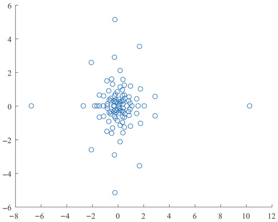
Figure 1. The spectrum of the randomly generated matrix pencil $A-\lambda B$ of order 100.

The Euclidean norms of A and B and the ranges of their elements are listed in Table 5. The values are rounded to five significant digits.

Table 5. Euclidean norms of A and B and the ranges of their elements for the randomly generated matrix pencil.

Norm of A	Norm of B	Range of A Elements	Range of B Elements
92.844	97.028	[3.0098e-05, 26.278]	[1.8548e-06, 30.360]

A MATLAB-executable, developed by the author, was used to perform the block diagonalization of the scaled matrix pencil $A-\lambda B$. The executable has an option to work on general matrices, or on matrices already reduced to the generalized Schur form [17], $\left(\tilde{A},\tilde{B}\right)$, with $\tilde{A}=Q^{T}AZ$, $\tilde{B}=Q^{T}BZ$, where Q and Z are orthogonal (hence, $Q^{T}Q=Q{Q}^T=I_n$ and $Z^{T}Z=Z{Z}^T=I_n$, with $I_n$ the identity matrix of order n); $\tilde{B}$ is upper triangular, and $\tilde{A}$ is block upper triangular with diagonal blocks of order 1 or 2, corresponding to real or complex conjugate eigenvalues, respectively. (All elements under the diagonal of $\tilde{B}$ and under the diagonal blocks of $\tilde{A}$ are zero.) The block diagonalization algorithm acts on $\tilde{A}$ and $\tilde{B}$. An essential part of the computations is the solution of a generalized Sylvester equation. Since this involves non-unitary transformations, their elements should be bounded, to ensure good accuracy. Specifically, if any of these elements exceeds a given threshold $\theta$, the process is stopped, and solving an enlarged Sylvester equation is tried. If many failed attempts are involved, the computational effort might be unacceptably high. Using the bound $\theta =5000$ and default options (the diagonal blocks are not reordered before each reduction step, the left and right transformations are updated), the algorithm computed the transformed matrix pencil $\widehat{A}-\lambda \widehat{B}$, with $\widehat{A}:={\widehat{Q}}^{T}A\widehat{Z}$, $\widehat{B}:={\widehat{Q}}^{T}B\widehat{Z}$, $\widehat{Q}=\tilde{Q}Q$, $\widehat{Z}=\tilde{Z}Z$, where $\tilde{Q}$ and $\tilde{Z}$ are the global transformations applied to $\tilde{A}$ and $\tilde{B}$ by the block diagonalization algorithm. The reduced matrix $\widehat{A}$ is block diagonal (see Figure 2), with diagonal blocks of order 1 and 2, while matrix $\widehat{B}$ is diagonal. There are 14 block pairs of order 1 and 43 block pairs of order 2. Since the original pencil has 14 real eigenvalues, the maximal possible reduction (with real arithmetic) was obtained.

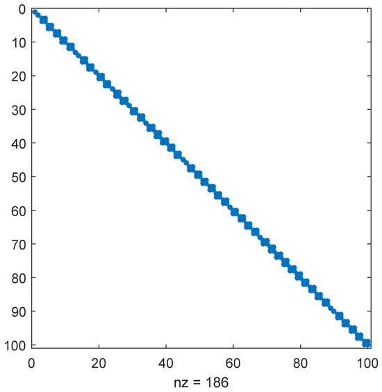
Figure 2. The form of the reduced matrix $\widehat{A}$ of the matrix pencil of order 100.

Let $e_a\left(A\right):=\parallel \widehat{A}-{\widehat{Q}}^{T}A\widehat{Z}\parallel$ and $e_a\left(B\right):=\parallel \widehat{B}-{\widehat{Q}}^{T}B\widehat{Z}\parallel$ be the absolute errors of $\widehat{A}$ and $\widehat{B}$ with respect to the transformed matrices ${\widehat{Q}}^{T}A\widehat{Z}$ and ${\widehat{Q}}^{T}B\widehat{Z}$, respectively, and let $e_r\left(A\right)$ and $e_r\left(B\right)$ be their relative errors, i.e., $e_r\left(A\right)=e_a\left(A\right)/\parallel A\parallel$, $e_r\left(B\right)=e_a\left(B\right)/\parallel B\parallel$, with $\parallel ·\parallel$ the Euclidean norm. Similarly, let $e_a\left(\lambda \right)$ and $e_r\left(\lambda \right)$ be the absolute and relative errors of the eigenvalues $\widehat{\lambda }$ of the matrix pencil $\widehat{A}-\lambda \widehat{B}$ with respect to the eigenvalues $\tilde{\lambda }$ of the matrix pencil $\tilde{A}-\lambda \tilde{B}$. If the eigenvalue problem is well conditioned, then $\tilde{\lambda }$ are very close to the true eigenvalues $\lambda$ of the matrix pencil $A-\lambda B$. These errors are reported in Table 6.

Table 6. Absolute and relative errors of the transformed matrices and eigenvalues.

${\mathit{e}}_{\mathit{a}}\left(\mathit{A}\right)$	${\mathit{e}}_{\mathit{a}}\left(\mathit{B}\right)$	${\mathit{e}}_{\mathit{r}}\left(\mathit{A}\right)$	${\mathit{e}}_{\mathit{r}}\left(\mathit{B}\right)$	${\mathit{e}}_{\mathit{a}}\left(\mathit{\lambda }\right)$	${\mathit{e}}_{\mathit{r}}\left(\mathit{\lambda }\right)$
2.2752e-14	1.4259e-14	2.4506e-16	1.4696e-16	2.0081e-15	9.9933e-17

All these errors are as good as possible for such a problem, which shows that the block diagonalization was successful. The reduced matrix pencil can be used efficiently instead of the original pencil, e.g., for computing matrix functions or the responses of a linear descriptor system. In this case, the input and output matrices of the system should be updated with the computed transformation matrices $\widehat{Q}$ and $\widehat{Z}$.

An example with dense clusters of eigenvalues. A matrix pencil of order $n=999$ with many clustered eigenvalues is considered now. The matrices A and B are already reduced to the generalized real Schur form. The spectrum is shown in Figure 3. It has 107 real and 446 complex conjugate eigenvalues.

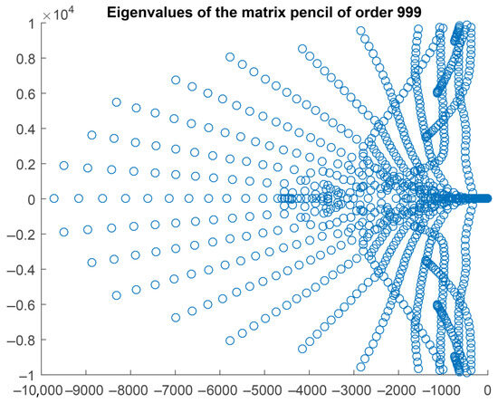
Figure 3. The spectrum of the matrix pencil $A-\lambda B$ of order 999 with dense clusters.

The Euclidean norms of A and B and the ranges of their elements are listed in Table 7. The values are rounded to five significant digits.

Table 7. Euclidean norms of A and B and the ranges of their elements for the matrix pencil of order 999 with dense clusters.

Norm of A	Norm of B	Range of A Elements	Range of B Elements
1.3936e-01	1.9073e-06	[0, 2.5123e-02]	[0, 4.2904e-07]

Using the approach described for the randomly generated example, a solution with 135 diagonal block pairs was computed in 62.68s (seconds). The largest block pair, of order 734, appeared in the 89-th block position on the diagonals; in addition, there are three $1\times 1$ and 131 2 × 2 diagonal block pairs. The remaining 104 real eigenvalues are included in the largest block pair.

Using an eigenvalue reordering strategy based on the pairwise “distances” between eigenvalues, measured by the approximate symmetric chordal metric, another solution was computed in 4.6905s; hence, the execution time was 13.36 times shorter. Specifically, 763 selected eigenvalues were moved to the leading positions, obtaining the matrices $\tilde{A}$ and $\tilde{B}$. The needed transformation matrices, $\tilde{Q}$ and $\tilde{Z}$, were computed. This reordering process, including the computation of $\tilde{Q}$ and $\tilde{Z}$, needed 2.4826s. The block diagonalization was then applied to the matrices $\tilde{A}$ and $\tilde{B}$, and it took 2.2078s. The relative errors in the transformed matrices and eigenvalues for the two computational stages are shown in Table 8.

Table 8. Relative errors of the transformed matrices and eigenvalues.

Stage	${\mathit{e}}_{\mathit{r}}\left(\mathit{A}\right)$	${\mathit{e}}_{\mathit{r}}\left(\mathit{B}\right)$	${\mathit{e}}_{\mathit{r}}\left(\mathit{\lambda }\right)$
Reordering	1.5935e-16	4.3898e-21	3.1502e-15
Block diagonalization	1.1542e-17	1.0614e-21	3.195e-15

Compared to the first approach, more block pairs, namely, 141, were found and the largest block pair, of order 719, appeared in the last position. This is the preferred situation, since well-separated eigenvalues could be quickly placed in small block pairs in the leading part, while big clusters remain to be placed in the trailing part of the matrix pencil. There were 140 2 × 2 block pairs; so, all real eigenvalues were available in the largest block pair. The efficiency gain is mainly due to better eigenvalue reordering, which reduced the number of failed attempts to solve the generalized Lyapunov equations. However, it is worth noting that the number of “distances” between eigenvalues is $n(n-1)/2=498501$; hence, it increases quadratically with the problem size. Therefore, it is important that the algorithms for computing the approximate symmetric chordal metric are as fast as possible.

The computed matrix $\widehat{A}$ has 140 $2\times 2$ diagonal blocks followed by a $719\times 719$ diagonal block. The matrix $\widehat{B}$ is diagonal with positive diagonal elements.

6. Conclusions

The basic theoretical properties of the approximate symmetric chordal metric for two real or complex numbers are investigated, and reliable, accurate, and efficient algorithms for its computation are proposed. A factored representation of the modulus of a complex number is introduced, which allows to obtain very accurate results for the entire range of the floating point number system of a computer. Two different ways to evaluate the distance between the reciprocals of the given numbers are described. The algorithms can be easily implemented on various architectures and compilers. Extensive numerical tests were performed to assess the performance of the associated implementation. The results were compared to those obtained in MATLAB, but with appropriate modifications for numbers very close to the bounds of the range of representable values, where the usual formulas give wrong results, as shown in several detailed numerical examples. As an application, the block diagonalization of matrix pencils is considered and two examples are investigated. The largest order example illustrates the efficiency improvement possible using a proper eigenvalue reordering strategy and fast algorithms for computing the approximate symmetric chordal metric. The algorithms can be used for applications using the chordal metric, if the triangle inequality is not required.

References

- Klamkin, M.S.; Meir, A. Ptolemy’s inequality, chordal metric, multiplicative metric. Pac. J. Math. 1982, 101, 389–392. [Google Scholar] [CrossRef][Green Version]
- Sasane, A. A generalized chordal metric in control theory making strong stabilizability a robust property. Complex Anal. Oper. Theory 2013, 7, 1345–1356. [Google Scholar] [CrossRef]
- Papadimitrakis, M. Notes on Complex Analysis. 2019. Available online: http://fourier.math.uoc.gr/~papadim/complex_analysis_2019/gca_vn_r.pdf (accessed on 3 May 2025).
- Rainio, O.; Vuorinen, M. Lipschitz constants and quadruple symmetrization by Möbius transformations. Complex Anal. Its Synerg. 2024, 20, 8. [Google Scholar] [CrossRef]
- Bishop, C. Complex Analysis I, MAT 536, Spring 2024; Stony Brook University, Dep Mathematics, 100 Nicolls Road: Stony Brook, NY, USA, 2024. [Google Scholar]
- Álvarez Tuñón, O.; Brodskiy, Y.; Kayacan, E. Loss it right: Euclidean and Riemannian metrics in learning-based visual odometry. arXiv 2023, arXiv:2401.05396. [Google Scholar] [CrossRef]
- Xu, W.; Pang, H.K.; Li, W.; Huang, X.; Guo, W. On the explicit expression of chordal metric between generalized singular values of Grassmann matrix pairs with applications. SIAM J. Matrix Anal. Appl. 2018, 39, 1547–1563. [Google Scholar] [CrossRef]
- Sun, J.-G. Perturbation theorems for generalized singular values. J. Comput. Math. 2025, 1, 233–242. [Google Scholar]
- Sasane, A. A refinement of the generalized chordal distance. SIAM J. Control Optim. 2014, 52, 3538–3555. [Google Scholar] [CrossRef][Green Version]
- Bavely, C.; Stewart, G.W. An algorithm for computing reducing subspaces by block diagonalization. SIAM J. Numer. Anal. 1979, 16, 359–367. [Google Scholar] [CrossRef][Green Version]
- Golub, G.H.; Van Loan, C.F. Matrix Computations, 4th ed.; The Johns Hopkins University Press: Baltimore, MD, USA, 2013. [Google Scholar]
- Wilkinson, J.H. The Algebraic Eigenvalue Problem; Oxford University Press (Clarendon): Oxford, UK, 1965. [Google Scholar]
- Wilkinson, J.H. Kronecker’s canonical form and the QZ algorithm. Linear Algebra Its Appl. 1979, 28, 285–303. [Google Scholar] [CrossRef]
- Stewart, G.W. On the sensitivity of the eigenvalue problem Ax = λBx. SIAM J. Numer. Anal. 1972, 9, 669–686. [Google Scholar] [CrossRef]
- Demmel, J.W. The condition number of equivalence transformations that block diagonalize matrix pencils. SIAM J. Numer. Anal. 1983, 20, 599–610. [Google Scholar] [CrossRef]
- Kågström, B.; Westin, L. Generalized Schur methods with condition estimators for solving the generalized Sylvester equation. IEEE Trans. Autom. Control 1989, 34, 745–751. [Google Scholar] [CrossRef]
- Anderson, E.; Bai, Z.; Bischof, C.; Blackford, S.; Demmel, J.; Dongarra, J.; Du Croz, J.; Greenbaum, A.; Hammarling, S.; McKenney, A.; et al. LAPACK Users’ Guide, 3rd ed.; Software·Environments·Tools, SIAM: Philadelphia, PA, USA, 1999. [Google Scholar]
- MathWorks®. MATLAB™, Release R2024b; The MathWorks, Inc.: Natick, MA, USA, 2024. [Google Scholar]
- Wolfram, S. The Story Continues: Announcing Version 14 of Wolfram Language and Mathematica. 2024. Available online: http://writings.stephenwolfram.com/2024/01/the-story-continues-announcing-version-14-of-wolfram-language-and-mathematica (accessed on 3 May 2025).
- Wang, B.; Kestelyn, X.; Kharazian, E.; Grolet, A. Application of Normal Form Theory to Power Systems: A Proof of Concept of a Novel Structure-Preserving Approach. In Proceedings of the 2024 IEEE Power & Energy Society General Meeting (PESGM), Seattle, WA, USA, 21–25 July 2024; pp. 1–5. [Google Scholar] [CrossRef]
- Malcolm, M.A. Algorithms to reveal properties of floating-point arithmetic. Commun. ACM 1972, 15, 949–951. [Google Scholar] [CrossRef]
- Gentleman, W.M.; Marovich, S.B. More on algorithms that reveal properties of floating point arithmetic units. Commun. ACM 1974, 17, 276–277. [Google Scholar] [CrossRef]
- Boyd, S.; Vandenberghe, L. Convex Optimization; Cambridge University Press: Cambridge, UK, 2004. [Google Scholar]
Disclaimer/Publisher’s Note: The statements, opinions and data contained in all publications are solely those of the individual author(s) and contributor(s) and not of MDPI and/or the editor(s). MDPI and/or the editor(s) disclaim responsibility for any injury to people or property resulting from any ideas, methods, instructions or products referred to in the content. |
© 2025 by the author. Licensee MDPI, Basel, Switzerland. This article is an open access article distributed under the terms and conditions of the Creative Commons Attribution (CC BY) license (https://creativecommons.org/licenses/by/4.0/).