Fuzzy-Valued Functions Calculus Through Midpoint Representation ^†

Abstract

In this paper, we are concerned with the calculus for fuzzy-valued functions of a single real variable when the adopted representation is the midpoint-radius; in particular, we extend the well-known LU-order to the more general case of the so-called $\gamma$-order based on the generalized Hukuhara difference and we show that the new index includes the commonly used order relations proposed in literature and it satisfies seven properties which play a crucial role in the justification of the main theorem based on the possibility to represent the efficient region through fuzzy-valued functions deeply related to the same region. Some graphical examples strengthen the innovative approach as a result of a generalization.

1. Introduction

The calculus for fuzzy-valued functions of a single real variable deserve more theoretical insights because of its potential to describe uncertainty through robust mathematical models.

In particular, we prefer to represent the calculus of fuzzy-valued functions of a single real variable through the midpoint-radius framework and we exploit the extension of the LU-order called $\gamma$-order-based (defined in [1]), which refers to the generalized Hukuhara difference studied in various works, including [2,3].

In general, the radius-midpoint notation has a wide field of application (see, for example, [4]) and, in particular in [5,6], using this midpoint-radius mode, some interesting applications in the field of interval-valued functions have been developed, providing a comprehensive overview of the theoretical properties associated with them which provide a solid foundation for extending these concepts to the case of fuzzy functions.

This attempt to consolidate the fuzzy case has already begun with two conference papers [7,8] presented at the 2020 IEEE International Conference on Fuzzy Systems (FUZZ-IEEE) and the 18th International Conference on Information Processing and Uncertainty Management in Knowledge-Based Systems (IPMU2020). Both papers specifically addressed the case of the LU-order.

The present work aims to further develop these contributions by providing a more comprehensive overview of the topics covered. It proposes a more detailed classification of the cases considered and, most importantly, extends the scope from the particular LU-order to the more general $\gamma$-order.

The structure of the paper is organized into six sections. Section 2 is dedicated to the introduction of notations and preliminary concepts related to midpoint representation. The principal ordering rules are elucidated in Section 3, whereas Section 4 discusses general properties of fuzzy-valued functions, including monotonicity, convexity, and periodicity. A comprehensive analysis of extrema for fuzzy-valued functions is presented in Section 5, and Section 6 provides the concluding remarks of the paper.

2. Midpoint Representation for Fuzzy Numbers

The family ${\mathcal{K}}_C$ of all bounded closed intervals in $\mathbb{R}$ is defined as the following set:

$${\mathcal{K}}_C=\left\{\left[a^{-},a^{+}\right]|a^{-},a^{+}\in \mathbb{R}\mathrm{and}{a}^{-}\le a^{+}\right\}$$

(1)

within which the midpoint-radius representation for a given interval $A=\left[a^{-},a^{+}\right]$ provides for the midpoint $\widehat{a}$ and radius $\tilde{a}$ defined as:

$$\widehat{a}={\displaystyle \frac{a^{+}+a^{-}}{2}}\mathrm{and}\tilde{a}={\displaystyle \frac{a^{+}-a^{-}}{2}}$$

(2)

where $a^{-}=\widehat{a}-\tilde{a}$ and $a^{+}=\widehat{a}+\tilde{a}$. An interval is denoted by $A=[a^{-},a^{+}]$ or, in midpoint notation, by $A=(\widehat{a};\tilde{a})$ and consequently ${\mathcal{K}}_C$ is also equal to

$${\mathcal{K}}_C=\left\{(\widehat{a};\tilde{a})|\widehat{a},\tilde{a}\in \mathbb{R}\mathrm{and}\tilde{a}\ge 0\right\}.$$

(3)

It follows that when an interval $C$ belongs to ${\mathcal{K}}_C$ then its elements are denoted as $c^{-},$ $c^{+},$ $\widehat{c},$ $\tilde{c}$, with $\tilde{c}\ge 0$, $c^{-}\le c^{+}$ and the interval by $C=[c^{-},c^{+}]$ in extreme-point representation or, equivalently, by $C=(\widehat{c};\tilde{c})$, in midpoint notation.

Given two intervals $A=[a^{-},a^{+}],B=[b^{-},b^{+}]\in {\mathcal{K}}_C$ and $\tau \in \mathbb{R}$, the following classical (Minkowski-type) addition, scalar multiplication and difference are defined:

• $A{\oplus }_{M}B=[a^{-}+b^{-},a^{+}+b^{+}]$,
• $\tau A=\{\tau a:a\in A\}=\left\{\begin{array}{cc}\left[\tau a^{-},\tau a^{+}\right],\hfill & \mathrm{if}\tau \ge 0\hfill \\ \left[\tau a^{+},\tau a^{-}\right],\hfill & \mathrm{if}\tau \le 0\hfill \end{array}\right.$,
• $-A=(-1)A=[-a^{+},-a^{-}]$,
• $A{\ominus }_{M}B=A{\oplus }_M(-1)B=[a^{-}-b^{+},a^{+}-b^{-}]$.

On the other hand, using midpoint notation, the above operations, for $A=(\widehat{a};\tilde{a}),B=(\widehat{b};\tilde{b})$ and $\tau \in \mathbb{R}$ become:

• $A{\oplus }_{M}B=(\widehat{a}+\widehat{b};\tilde{a}+\tilde{b})$,
• $\tau A=(\tau \widehat{a};|\tau \left|\tilde{a}\right)$,
• $-A=(-\widehat{a};\tilde{a})$,
• $A{\ominus }_{M}B=(\widehat{a}-\widehat{b};\tilde{a}+\tilde{b})$.

In what follows, the subscript ${(·)}_M$, indicating the Minkowski-type operations, is used just when misunderstandings may arise.

The generalized Hukuhara difference ($gH$-difference for short, as extensively detailed in [3,9]) of two intervals A and B always exists and it is denoted by

$$A{\ominus }_{gH}B=C⟺(A=B{\oplus }_{M}C\mathrm{or}B=A{\ominus }_{M}C)$$

(4)

or, using midpoint notation, by

$$A{\ominus }_{gH}B=(\widehat{a}-\widehat{b};|\tilde{a}-\tilde{b}\left|\right)\subseteq A{\ominus }_{M}B.$$

(5)

Similarly, we have that the $gH$-addition for intervals is also defined by

$$A{\oplus }_{gH}B=A{\ominus }_{gH}(-B)=(\widehat{a}+\widehat{b};|\tilde{a}-\tilde{b}\left|\right)\subseteq A{\oplus }_{M}B.$$

(6)

Furthermore, if $A\in {\mathcal{K}}_C$, the length of interval A will be denoted by $len\left(A\right)=a^{+}-a^{-}=2\widehat{a}$.

In addition, given two intervals $A,B\in {\mathcal{K}}_C$, the Pompeiu–Hausdorff distance $d_H:{\mathcal{K}}_C\times {\mathcal{K}}_C\to {\mathbb{R}}^{+}\cup \left\{0\right\}$ is:

$$d_H(A,B)=\max \left\{\underset{a\in A}{\max }d(a,B),\underset{b\in B}{\max }d(b,A)\right\}$$

(7)

where $d(a,B)={\min }_{b\in B}|a-b|$; it is established (see [3]) that $d_H(A,B)=∥A{\ominus }_{gH}B∥$ and for $A,B\in {\mathcal{K}}_C$ it holds that

$$d_H(A,B)=0\iff A{\ominus }_{gH}B=0\iff A=B.$$

(8)

and $({\mathcal{K}}_C,d_H)$ is a complete metric space.

The concept of fuzzy set, of which [10] is a key element, is also part of the preliminary notions useful for evaluating the contribution of the article.

Definition 1

([11]). A fuzzy set on $\mathbb{R}$ is a mapping $u:\mathbb{R}\to [0,1]$ and its α-level set are defined as ${\left[u\right]}_{\alpha }=\left\{x\in \mathbb{R}:u\left(x\right)\ge \alpha \right\}$ for any $\alpha \in [0,1]$. The support is defined as: $supp\left(u\right)=\left\{x\in \mathbb{R}\left|u\right(x)>0\right\}$; the 0-level set of u is defined by ${\left[u\right]}_0=cl\left(supp\left(u\right)\right)$ where $cl\left(M\right)$ means the closure of the subset $M\subset \mathbb{R}$.

A fuzzy set $\mathit{u}$ on $\mathbb{R}$ is called a fuzzy number when:

• u is normal, i.e., there exists $x_0\in \mathbb{R}$ such that $u\left(x_0\right)=1,$
• u is a convex fuzzy set (i.e., $u(tx+(1-t\left)y\right)\ge \min \left\{u\right(x),u(y\left)\right\},\forall t\in [0,1],x,y\in \mathbb{R}$),
• u is upper semi-continuous on $\mathbb{R}$,
• $cl\{x\in \mathbb{R}|u\left(x\right)>0\}$ is compact.

If ${\mathbb{R}}_{\mathit{F}}$ denotes the family of fuzzy numbers, then for any $u\in {\mathbb{R}}_{\mathit{F}}$ it holds ${\left[u\right]}_{\alpha }\in {\mathbb{K}}_{\mathit{C}}$ for all $\alpha \in [0,1]$, and thus, the $\alpha$-levels of a fuzzy number are given by ${\left[u\right]}_{\alpha }=[u_{\alpha }^{-},u_{\alpha }^{+}]$, $u_{\alpha }^{-},u_{\alpha }^{+}\in \mathbb{R}$ for all $\alpha \in [0,1]$. In midpoint notation, we write ${\left[u\right]}_{\alpha }=({\widehat{u}}_{\alpha },{\tilde{u}}_{\alpha })$ where ${\widehat{u}}_{\alpha }={\displaystyle \frac{u_{\alpha }^{+}+u_{\alpha }^{-}}{2}}\mathrm{and}{\tilde{u}}_{\alpha }={\displaystyle \frac{u_{\alpha }^{+}-u_{\alpha }^{-}}{2}}$ so that $u_{\alpha }^{-}={\widehat{u}}_{\alpha }-{\tilde{u}}_{\alpha }$ and $u_{\alpha }^{+}={\tilde{u}}_{\alpha }+{\widehat{u}}_{\alpha }.$ Triangular fuzzy numbers are well determined by three real numbers $a\le b\le c$, denoted by $u=<a,b,c>$, with $\alpha$-levels ${\left[u\right]}_{\alpha }=[a+(b-a)\alpha ,c-(c-b)\alpha ]$ for all $\alpha \in [0,1]$.

It is well known that in terms of $\alpha$-levels, and taking into account the midpoint notation, for every $\alpha \in [0,1]$ the following definitions hold:

$${[u+v]}_{\alpha }={\left[u\right]}_{\alpha }+{\left[v\right]}_{\alpha }=[u_{\alpha }^{-}+v_{\alpha }^{-},u_{\alpha }^{+}+v_{\alpha }^{+}]=({\widehat{u}}_{\alpha }+{\widehat{v}}_{\alpha };{\tilde{u}}_{\alpha }+{\tilde{v}}_{\alpha })$$

(9)

and

$${\left[\lambda u\right]}_{\alpha }=\left[\min \{\lambda u_{\alpha }^{-},\lambda u_{\alpha }^{+}\},\max \{\lambda u_{\alpha }^{-},\lambda u_{\alpha }^{+}\}\right]=(\lambda {\widehat{u}}_{\alpha };\left|\lambda \right|{\tilde{u}}_{\alpha }).$$

(10)

The Level-wise gH (LgH)-difference can be read as a generalization of the fuzzy gH-difference.

Definition 2.

For given two fuzzy numbers $u,v\in {\mathbb{R}}_{\mathit{F}}$, the LgH-difference of $u,v$ is defined as the family of interval-valued gH-differences defined as:

$$w=u{\ominus }_{LgH}v=\left\{W_{\alpha }={\left[u\right]}_{\alpha }{\ominus }_{gH}{\left[v\right]}_{\alpha }\forall \alpha \in [0,1]\right\},$$

(11)

that is, for each $\alpha \in [0,1]$, either ${\left[u\right]}_{\alpha }={\left[v\right]}_{\alpha }+W_{\alpha }$ or ${\left[v\right]}_{\alpha }={\left[u\right]}_{\alpha }+(-1)W_{\alpha }$.

In relation with the defined difference, we detail the concept of LgH-differentiability.

Definition 3

([9]). Let $x_0\in ]a,b[$ and h be such that $x_0+h\in ]a,b[$, then the LgH-derivative of a function $F:]a,b[\to {\mathbb{R}}_{\mathit{F}}$ at $x_0$ is defined as the set of interval-valued gH-derivatives, if they exist,

$$F_{LgH}^{\prime }{\left(x_0\right)}_{\alpha }=\underset{h\to 0}{\lim }{\displaystyle \frac{1}{h}}\left({\left[F(x_0+h)\right]}_{\alpha }{\ominus }_{gH}{\left[F\left(x_0\right)\right]}_{\alpha }\right)$$

(12)

If $F_{LgH}^{\prime }{\left(x_0\right)}_{\alpha }$ is a compact interval for all $\alpha \in [0,1],$ we say that F is LgH-differentiable at $x_0$ and the family of intervals $\left\{F_{LgH}^{\prime }{\left(x_0\right)}_{\alpha }|\alpha \in [0,1]\right\}$ is the LgH-derivative of F at $x_0$, denoted by $F_{LgH}^{\prime }\left(x_0\right).$

Also, one-side derivatives can be considered. The right gH-derivative of F at $x_0$ is

$$F_{\left(r\right)LgH}^{\prime }{\left(x_0\right)}_{\alpha }=\underset{h\searrow 0}{\lim }{\displaystyle \frac{1}{h}}\left({\left[F(x_0+h)\right]}_{\alpha }{\ominus }_{LgH}{\left[F\left(x_0\right)\right]}_{\alpha }\right)$$

(13)

while to the left it is defined as

$$F_{\left(l\right)LgH}^{\prime }\left(x_0\right)=\underset{h\nearrow 0}{\lim }{\displaystyle \frac{1}{h}}\left({\left[F(x_0+h)\right]}_{\alpha }{\ominus }_{gH}{\left[F\left(x_0\right)\right]}_{\alpha }\right)$$

(14)

The LgH-derivative exists at $x_0$ if and only if the left and right derivatives at $x_0$ exist and produce the same interval.

In terms of midpoint representation ${\left[F\left(x\right)\right]}_{\alpha }=\left({\widehat{f}}_{\alpha }\left(x\right);{\tilde{f}}_{\alpha }\left(x\right)\right)$, for all $\alpha \in [0,1]$, we can write

$$\begin{array}{ccc}\hfill {\displaystyle \frac{{F(x+h)]}_{\alpha }{\ominus }_{gH}{\left[F\left(x\right)\right]}_{\alpha }}{h}}& =& \left({\widehat{\Delta }}_{gH}{F}_{\alpha }(x,h);{\tilde{\Delta }}_{gH}{F}_{\alpha }(x,h)\right)\mathrm{where}\hfill \end{array}$$

(15)

$$\begin{array}{ccc}\hfill {\widehat{\Delta }}_{gH}{F}_{\alpha }(x,h)& =& {\displaystyle \frac{{\widehat{f}}_{\alpha }(x+h)-{\widehat{f}}_{\alpha }\left(x\right)}{h}},\hfill \end{array}$$

(16)

$$\begin{array}{ccc}\hfill {\tilde{\Delta }}_{gH}{F}_{\alpha }(x,h)& =& \left|{\displaystyle \frac{{\tilde{f}}_{\alpha }(x+h)-{\tilde{f}}_{\alpha }\left(x\right)}{h}}\right|\hfill \end{array}$$

(17)

and taking the limit for $h⟶0$, we obtain the LgH-derivative of $F_{\alpha }$, if and only if the two limits $\underset{h⟶0}{\lim }{\displaystyle \frac{{\widehat{f}}_{\alpha }(x+h)-{\widehat{f}}_{\alpha }\left(x\right)}{h}}$ and $\underset{h⟶0}{\lim }\left|{\displaystyle \frac{{\tilde{f}}_{\alpha }(x+h)-{\tilde{f}}_{\alpha }\left(x\right)}{h}}\right|$ exist in $\mathbb{R}$; we remark that the midpoint function ${\widehat{f}}_{\alpha }$ is required to admit the ordinary derivative at x. With respect to the existence of the second limit, the existence of the left and right derivatives ${\tilde{f}}_{l-\alpha }^{\prime }\left(x\right)$ and ${\tilde{f}}_{r-\alpha }^{\prime }\left(x\right)$ is required with $\left|{\tilde{f}}_{l-\alpha }^{\prime }\left(x\right)\right|=\left|{\tilde{f}}_{r-\alpha }^{\prime }\left(x\right)\right|={\tilde{w}}_{\alpha }\left(x\right)\ge 0$ (in particular ${\tilde{w}}_{\alpha }\left(x\right)=\left|{\tilde{f}}_{\alpha }^{\prime }\left(x\right)\right|$ if ${\tilde{f}}_{\alpha }^{\prime }\left(x\right)$ exists) so that we have

$$F_{LgH}^{\prime }{\left(x\right)}_{\alpha }=\left({\widehat{f}}_{\alpha }^{\prime }\left(x\right);{\tilde{w}}_{\alpha }\left(x\right)\right)$$

(18)

or, in the standard interval notation,

$$F_{LgH}^{\prime }{\left(x\right)}_{\alpha }=\left[{\widehat{f}}_{\alpha }^{\prime }\left(x\right)-{\tilde{w}}_{\alpha }\left(x\right),{\widehat{f}}_{\alpha }^{\prime }\left(x\right)+{\tilde{w}}_{\alpha }\left(x\right)\right].$$

(19)

3. Orders for Fuzzy Numbers

Regarding the partial order for intervals, the LU-fuzzy partial order is well known in the literature and we can find a complete investigation in [12]; Ref. [1] also introduces a more general $\gamma$-order based on the gH-difference that includes the generally used order relations and allows the definition of risk measures to quantify a worst-case loss in interval maximization or minimization problems.

To facilitate understanding of the text, we present some of the key definitions related to these interval orders.

Specifically, consider two intervals $A=[a^{-},a^{+}]=(\widehat{a};\tilde{a})$ and $B=[b^{-},b^{+}]=(\widehat{b};\tilde{b})\in {\mathcal{K}}_{\mathcal{C}}$. We then define the Lower and Upper order (abbreviated as the $LU$-order), denoted by ${⪷}_{LU}$, as follows:

$$A{⪷}_{LU}B\iff a^{-}⩽b^{-}\mathrm{and}{a}^{+}⩽b^{+}.$$

(20)

However, we can further refine the definition by incorporating the cases of strict order and strong order, exactly as reported in [5,6].

The subsequent definition extends the statement made in (20).

Definition 4

([5]). Given $A=[a^{-},a^{+}]\in {\mathcal{K}}_C$, $B=[b^{-},b^{+}]\in {\mathcal{K}}_C$, we say that

(i) 

$A{⪷}_{LU}B$ if and only if $a^{-}⩽b^{-}$ and $a^{+}⩽b^{+}$,

(ii) 

$A{\precsim }_{LU}B$ if and only if $A{⪷}_{LU}B$ and ($a^{-}<b^{-}$ or $a^{+}<b^{+}$),

(iii) 

$A{\prec }_{LU}B$ if and only if $a^{-}<b^{-}$ and $a^{+}<b^{+}$.

Using midpoint notation $A=(\widehat{a};\tilde{a})$, $B=(\widehat{b};\tilde{b})$, the partial orders $\left(i\right)$ and $\left(iii\right)$ above can be expressed as

$$\left(i\right)\left\{\begin{array}{c}\widehat{a}⩽\widehat{b}\\ \tilde{b}⩽\tilde{a}+(\widehat{b}-\widehat{a})\\ \tilde{b}⩾\tilde{a}-(\widehat{b}-\widehat{a})\end{array}\right.\mathrm{and}\left(iii\right)\left\{\begin{array}{c}\widehat{a}<\widehat{b}\\ \tilde{b}<\tilde{a}+(\widehat{b}-\widehat{a})\\ \tilde{b}>\tilde{a}-(\widehat{b}-\widehat{a})\end{array}\right.$$

while the partial order $\left(ii\right)$ can be expressed in terms of $\left(i\right)$ with the additional requirement that at least one of the inequalities is strict.

The three order relations ${⪷}_{LU}$, ${\precsim }_{LU}$ and ${\prec }_{LU}$ can be generalized on the basis of the $gH$-difference as follows.

Definition 5

([6]). Given two intervals $A=\left[a^{-},a^{+}\right]=\left(\widehat{a};\tilde{a}\right)$ and $B=\left[b^{-},b^{+}\right]=(\widehat{b};\tilde{b})$ and ${\gamma }^{-}⩽0$, ${\gamma }^{+}⩾0$ (eventually ${\gamma }^{-}=-\infty$ and/or ${\gamma }^{+}=+\infty$) we define the following order relation, denoted ${⪷}_{{\gamma }^{-},{\gamma }^{+}}$,

$$A{⪷}_{{\gamma }^{-},{\gamma }^{+}}B⟺\left\{\begin{array}{c}\widehat{a}⩽\widehat{b}\\ \tilde{a}⩾\tilde{b}+{\gamma }^{+}\left(\widehat{a}-\widehat{b}\right)\\ \tilde{a}⩽\tilde{b}+{\gamma }^{-}\left(\widehat{a}-\widehat{b}\right),\end{array}\right.$$

(21)

similarly, we define the following (strict) order relation, denoted ${\precsim }_{{\gamma }^{-},{\gamma }^{+}}$,

$$A{\precsim }_{{\gamma }^{-},{\gamma }^{+}}B⟺\left\{\begin{array}{c}\widehat{a}<\widehat{b}\\ \tilde{a}⩾\tilde{b}+{\gamma }^{+}\left(\widehat{a}-\widehat{b}\right)\\ \tilde{a}⩽\tilde{b}+{\gamma }^{-}\left(\widehat{a}-\widehat{b}\right)\end{array}\right.$$

(22)

and the following (strong) order relation, denoted ${\prec }_{{\gamma }^{-},{\gamma }^{+}}$,

$$A{\prec }_{{\gamma }^{-},{\gamma }^{+}}B⟺\left\{\begin{array}{c}\widehat{a}<\widehat{b}\\ \tilde{a}>\tilde{b}+{\gamma }^{+}\left(\widehat{a}-\widehat{b}\right)\\ \tilde{a}<\tilde{b}+{\gamma }^{-}\left(\widehat{a}-\widehat{b}\right).\end{array}\right.$$

(23)

At this point, extending what is reported in [13] to its corresponding fuzzy version, it is interesting to further expand the cases relating to the $\gamma$-order, analyzing the entire spectrum of possibilities that the two real values ${\gamma }^{-}$ and ${\gamma }^{+}$ can assume.

Therefore, let ${\gamma }^{-},{\gamma }^{+}\in \mathbb{R}\cup \{\pm \infty \}$ with ${\gamma }^{-}⩽{\gamma }^{+}$, if we consider $u\in {\mathbb{R}}_{\mathcal{F}}$ and the corresponding level-wise expressed in midpoint notation $u_{\alpha }=({\widehat{u}}_{\alpha };{\tilde{u}}_{\alpha })$, for each $\alpha \in [0,1]$, we are able to define three relations between u and a generic fuzzy number $z\in {\mathbb{R}}_{\mathcal{F}}$, with $z_{\alpha }=({\widehat{z}}_{\alpha };{\tilde{z}}_{\alpha })$; in [14] the following equivalences are established:

$$z_{\alpha }{⪷}_{{\gamma }^{-}{\gamma }^{+}}^{*}{u}_{\alpha }\iff$$

$$\left(1\right)if{\gamma }^{-}⩽{\gamma }^{+}<0:\left\{\begin{array}{c}{\tilde{z}}_{\alpha }⩽{\tilde{u}}_{\alpha }+{\gamma }^{-}({\widehat{x}}_{\alpha }-{\widehat{u}}_{\alpha })\\ {\tilde{z}}_{\alpha }⩽{\tilde{u}}_{\alpha }+{\gamma }^{+}({\widehat{x}}_{\alpha }-{\widehat{u}}_{\alpha })\end{array}\right.$$

(24)

$$\left(2\right)if0<{\gamma }^{-}⩽{\gamma }^{+}:\left\{\begin{array}{c}{\tilde{z}}_{\alpha }⩾{\tilde{u}}_{\alpha }+{\gamma }^{-}({\widehat{x}}_{\alpha }-{\widehat{u}}_{\alpha })\\ {\tilde{z}}_{\alpha }⩾{\tilde{u}}_{\alpha }+{\gamma }^{+}({\widehat{x}}_{\alpha }-{\widehat{u}}_{\alpha })\end{array}\right.$$

(25)

while in [1] we write the equivalence in the following form (where the conditions ${\widehat{z}}_{\alpha }⩽{\widehat{u}}_{\alpha }$, is added when ${\gamma }^{-}=-\infty ,{\gamma }^{+}=+\infty$ or ${\gamma }^{-}=0,{\gamma }^{+}=0$):

$$z_{\alpha }{⪷}_{{\gamma }^{-}{\gamma }^{+}}^{*}{u}_{\alpha }\iff$$

$$\begin{array}{cc}& \left(3\right)if{\gamma }^{-}⩽0,{\gamma }^{+}⩾0:\left\{\begin{array}{c}{\tilde{z}}_{\alpha }⩾{\tilde{u}}_{\alpha }+{\gamma }^{-}({\widehat{x}}_{\alpha }-{\widehat{u}}_{\alpha })\\ {\tilde{z}}_{\alpha }⩽{\tilde{u}}_{\alpha }+{\gamma }^{+}({\widehat{x}}_{\alpha }-{\widehat{u}}_{\alpha })\end{array}\right.\end{array}$$

(26)

The third case can be analyzed in a more detailed way; given the conditions in case (3): ${\gamma }^{-}⩽0,{\gamma }^{+}⩾0,$ the order relation denoted as ${⪷}_{{\gamma }^{-},{\gamma }^{+}}$ can be defined as follows:

$$z_{\alpha }{⪷}_{{\gamma }^{-},{\gamma }^{+}}{u}_{\alpha }⟺\left\{\begin{array}{c}{\tilde{z}}_{\alpha }⩽{\tilde{u}}_{\alpha }+{\gamma }^{-}\left({\widehat{x}}_{\alpha }-{\widehat{u}}_{\alpha }\right)\\ {\tilde{z}}_{\alpha }⩾{\tilde{u}}_{\alpha }+{\gamma }^{+}\left({\widehat{x}}_{\alpha }-{\widehat{u}}_{\alpha }\right)\end{array}\right.$$

(27)

i.e.,

$$z_{\alpha }{⪷}_{{\gamma }^{-},{\gamma }^{+}}{u}_{\alpha }⟺\left\{\begin{array}{c}{\tilde{x}}_{\alpha }-{\gamma }^{-}{\widehat{x}}_{\alpha }⩽{\tilde{u}}_{\alpha }-{\gamma }^{-}{\widehat{u}}_{\alpha }\\ {\tilde{x}}_{\alpha }-{\gamma }^{+}{\widehat{x}}_{\alpha }⩾{\tilde{u}}_{\alpha }-{\gamma }^{+}{\widehat{u}}_{\alpha }\end{array}\right.$$

(28)

Moreover, as it will be better defined below (see Definition 8), for a given fuzzy number $u_{\alpha }=({\widehat{u}}_{\alpha };{\tilde{u}}_{\alpha })$, it is possible to introduce the following sets of fuzzy numbers $z_{\alpha }$:

$\left({⪷}_{{\gamma }^{-},{\gamma }^{+}}\right)$-dominated by $u_{\alpha }$: $\{z_{\alpha }\in {\mathbb{R}}_{\mathcal{F}}|u_{\alpha }{⪷}_{{\gamma }^{-},{\gamma }^{+}}{x}_{\alpha }\},$

$\left({⪷}_{{\gamma }^{-},{\gamma }^{+}}\right)$-dominating $u_{\alpha }$: $\{z_{\alpha }\in {\mathbb{R}}_{\mathcal{F}}|x_{\alpha }{⪷}_{{\gamma }^{-},{\gamma }^{+}}{u}_{\alpha }\},$

$\left({⪷}_{{\gamma }^{-},{\gamma }^{+}}\right)$-incomparable with $u_{\alpha }$ when $z_{\alpha }\in {\mathbb{R}}_{\mathcal{F}}$, but it does not belong to any of the two previous sets.

Note also that by changing ${\gamma }^{-}⩽0$ and ${\gamma }^{+}⩾0$, we obtain an infinite number of partial orders and by increasing ${\gamma }^{+}⩾0$ and/or decreasing ${\gamma }^{-}⩽0$, the incomparability region(s) will be reduced.

Now we will consider only case 3 ( ${\gamma }^{-}⩽0,{\gamma }^{+}⩾0$) because of its significance in estimating the risk of possible worst-case loss (see [11,15,16]); indeed, it is possible to face two types of risk, due to the possibility of a worst-case loss if we make a choice exclusively on the basis of the midpoint values $\widehat{x}$ and $\widehat{u}$.

In many real-life situations, we need to select an appropriate action. In economics, a reasonable idea is to select an action that leads to the largest values of the expected gain because if we repeatedly make such a selection, then, because of the law of large numbers, we will obtain the largest possible gain.

Moreover, according to [14], it appears evident that for all $u,v\in {\mathbb{R}}_{\mathcal{F}}$, where $u=[u^{-},u^{+}]=(\widehat{u};\tilde{u})$ and $v=[v^{-},v^{+}]=(\widehat{v};\tilde{v})$ according to endpoint and midpoint notations, respectively, the following properties are satisfied:

• reflexivity: $u⩽u$, for all $u\in {\mathbb{R}}_{\mathcal{F}}$;
• antisymmetry: $u⩽v$ and $v⩽u$ iff $u=v$, for all $u,v\in {\mathbb{R}}_{\mathcal{F}}$;
• transitivity: $u⩽v$ and $v⩽w$, then $u⩽w$, for all $u,v,w\in {\mathbb{R}}_{\mathcal{F}}$;
• consistency with common sense: if $u^{+}⩽v^{-}$ then $u⩽v$, for all $u,v\in {\mathbb{R}}_{\mathcal{F}}$;
• scale-invariance: if $u⩽v$ then $cu⩽cv$, for all $u,v\in {\mathbb{R}}_{\mathcal{F}}$ (that is, if we multiply all the gains by the same positive constant $c>0$, then whichever gain was larger remains larger, and whichever gain was smaller remains smaller);
• additivity: $u⩽v$ iff $u+c⩽v+c$ for all $u,v,c\in {\mathbb{R}}_{\mathcal{F}}$ (that is, if we add the same amount to the two gains, this will not change which gain is larger);
• closeness: when the values of $u^{-}$ and $u^{+}$ are close, the corresponding alternatives are practically indistinguishable. Similarly, if we have two sequences ${\left(u\right)}_n$ and ${\left(v\right)}_n$ so that ${\left(u\right)}_n⩽{\left(v\right)}_n$ and endpoints of both tends to some limits, then, since the limit intervals are indistinguishable from these ones for sufficiently large n, we should expect the same relation ⩽ for the limit intervals. This means that if ${\left(u\right)}_n⩽{\left(v\right)}_n$ for all n, and ${\left(u\right)}_n^{-}⟶u^{-}$, ${\left(u\right)}_n^{+}⟶u^{+}$, ${\left(v\right)}_n^{-}⟶v^{-}$, ${\left(v\right)}_n^{+}⟶v^{+}$, then $u⩽v$.

From now on the symbol ⪷ will be used to indicate ${⪷}_{{\gamma }^{-},{\gamma }^{+}}$, with ${\gamma }^{-}⩽0,{\gamma }^{+}⩾0$ and, in addition to the ⪷-order, we will also consider the relations of strict order, indicated by ≾, and of strong order, indicated by ≺, which, respectively, stand for ${\precsim }_{{\gamma }^{-},{\gamma }^{+}}$ and ${\prec }_{{\gamma }^{-},{\gamma }^{+}}$.

We point out that, given $u,v\in {\mathbb{R}}_{\mathcal{F}}$ and $\alpha \in [0,1]$, we write their $\alpha$-levels in endpoint notation as $u_{\alpha }=[u_{\alpha }^{-},u_{\alpha }^{+}]\in {\mathbb{K}}_{\mathit{C}}$ and $v_{\alpha }=[v_{\alpha }^{-},v_{\alpha }^{+}]\in {\mathbb{K}}_{\mathit{C}}$, respectively.

Definition 6.

Given u,$v\in {\mathbb{R}}_{\mathcal{F}}$ and given $\alpha \in [0,1],$ we say that

1.

$u{⪷}_{\alpha }v$ if and only if $u_{\alpha }⪷v_{\alpha },$ that is, $u_{\alpha }^{-}\le v_{\alpha }^{-}$ and $u_{\alpha }^{+}\le v_{\alpha }^{+}$,

2.

$u{\precsim }_{\alpha }v$ if and only if $u_{\alpha }\precsim v_{\alpha },$

3.

$u{\prec }_{\alpha }v$ if and only if $u_{\alpha }\prec v_{\alpha }.$

Correspondingly, the analogous $({\gamma }^{-},{\gamma }^{+})$-fuzzy orders can be obtained by

4.

$u⪷v$ if and only if $u{⪷}_{\alpha }v$ for all $\alpha \in [0,1],$

5.

$u\precsim v$ if and only if $u{\precsim }_{\alpha }v$ for all $\alpha \in [0,1],$

6.

$u\prec v$ if and only if $u{\prec }_{\alpha }v$ for all $\alpha \in [0,1].$

The corresponding reverse orders are, respectively, $u⪸v\iff v⪷u$, $u\succsim v\iff v\precsim u$ and $u\succ v\iff v\prec u$.

Switching to the $\alpha$-levels midpoint notation $u_{\alpha }=({\widehat{u}}_{\alpha };{\tilde{u}}_{\alpha })$, $v_{\alpha }=({\widehat{v}}_{\alpha };{\tilde{v}}_{\alpha })$ for all $\alpha \in [0,1]$, the partial orders $(1.)$ and $(3.)$ above can be written for all $\alpha \in [0,1]$ as

$$\begin{array}{ccc}& & \left(i\right)\left\{\begin{array}{c}{\widehat{u}}_{\alpha }\le {\widehat{v}}_{\alpha }\\ {\tilde{v}}_{\alpha }\le {\tilde{u}}_{\alpha }+{\gamma }^{+}({\widehat{v}}_{\alpha }-{\widehat{u}}_{\alpha })\\ {\tilde{v}}_{\alpha }\ge {\tilde{u}}_{\alpha }-{\gamma }^{-}({\widehat{v}}_{\alpha }-{\widehat{u}}_{\alpha })\end{array}\right.\mathrm{and}\hfill \end{array}$$

(29)

$$\begin{array}{ccc}& & \left(iii\right)\left\{\begin{array}{c}{\widehat{u}}_{\alpha }<{\widehat{v}}_{\alpha }\\ {\tilde{v}}_{\alpha }<{\tilde{u}}_{\alpha }+{\gamma }^{+}({\widehat{v}}_{\alpha }-{\widehat{u}}_{\alpha })\\ {\tilde{v}}_{\alpha }>{\tilde{u}}_{\alpha }-{\gamma }^{-}({\widehat{v}}_{\alpha }-{\widehat{u}}_{\alpha })\end{array}\right.;\hfill \end{array}$$

(30)

then, adding the requirement that at least one of the two inequalities be strict, we can express the partial order (2.) in terms of $\left(i\right)$.

The results listed below are obtained from those in [5,6] for each $\alpha \in [0,1]$, where proof can be found, too. Indeed, the level-wise generalized Hukuhara difference (LgH-difference), which was used in the fuzzy case, turns out to be more general than the gH-difference of the interval case, but if we consider the $\alpha$-levels of the fuzzy version, then we have that the properties as in the interval case are confirmed; therefore, all the relations and properties established in the above-mentioned papers are maintained.

Proposition 1.

Let $u,v\in {\mathbb{R}}_{\mathcal{F}}$ with $u_{\alpha }=({\widehat{u}}_{\alpha };{\tilde{u}}_{\alpha }),v_{\alpha }=({\widehat{v}}_{\alpha };{\tilde{v}}_{\alpha })$ for all $\alpha \in [0,1]$. We have

1.

$u⪷v$ if and only if ${\widehat{v}}_{\alpha }-{\widehat{u}}_{\alpha }\ge \left|{\tilde{v}}_{\alpha }-{\tilde{u}}_{\alpha }\right|$;

2.

$u\precsim v$ if and only if ${\widehat{u}}_{\alpha }<{\widehat{v}}_{\alpha }$ and ${\widehat{v}}_{\alpha }-{\widehat{u}}_{\alpha }\ge \left|{\tilde{v}}_{\alpha }-{\tilde{u}}_{\alpha }\right|$;

3.

$u\prec v$ if and only if ${\widehat{v}}_{\alpha }-{\widehat{u}}_{\alpha }>\left|{\tilde{v}}_{\alpha }-{\tilde{u}}_{\alpha }\right|$;

4.

$u⪸v$ if and only if ${\widehat{u}}_{\alpha }-{\widehat{v}}_{\alpha }\ge \left|{\tilde{v}}_{\alpha }-{\tilde{u}}_{\alpha }\right|$;

5.

$u\succsim v$ if and only if ${\widehat{u}}_{\alpha }>{\widehat{v}}_{\alpha }$ and ${\widehat{u}}_{\alpha }-{\widehat{v}}_{\alpha }\ge \left|{\tilde{v}}_{\alpha }-{\tilde{u}}_{\alpha }\right|$;

6.

$u\succ v$ if and only if ${\widehat{u}}_{\alpha }-{\widehat{v}}_{\alpha }>\left|{\tilde{v}}_{\alpha }-{\tilde{u}}_{\alpha }\right|$.

When case 3 is verified (if $\gamma$ > 0 then we consider ${\gamma }^{+}=-{\gamma }^{-}$), we have that the following holds.

Proposition 2.

Let $u,v\in {\mathbb{R}}_{\mathcal{F}}$ with $u_{\alpha }=({\widehat{u}}_{\alpha };{\tilde{u}}_{\alpha })$, $v_{\alpha }=({\widehat{v}}_{\alpha };{\tilde{v}}_{\alpha })$ for all $\alpha \in [0,1]$. We have

1.

$u⪷v$ if and only if $u{\ominus }_{LgH}v⪷0$;

2.

$u\precsim v$ if and only if $u{\ominus }_{LgH}v\precsim 0$;

3.

$u\prec v$ if and only if $u{\ominus }_{LgH}v\prec 0$;

4.

$u⪸v$ if and only if $u{\ominus }_{LgH}v⪸0$;

5.

$u\succsim v$ if and only if $u{\ominus }_{LgH}v\succsim 0$;

6.

$u\succ v$ if and only if $u{\ominus }_{LgH}v\succ 0$.

Definition 7.

Given $u,v\in {\mathbb{R}}_{\mathit{F}}$, we clearly have that

$$\begin{array}{cc}\hfill u& \prec v\Rightarrow u\precsim v\Rightarrow u⪷v\hfill \\ \hfill u& \succ v\Rightarrow u\succsim v\Rightarrow u⪸v.\hfill \end{array}$$

(31)

We say that u and v are incomparable if neither $u⪷v$ nor $u⪸v$ and u and v are α-incomparable if neither $u{⪷}_{\alpha }v$ nor $u{⪸}_{\alpha }v.$

Proposition 3.

Let $u,v\in {\mathbb{R}}_{\mathcal{F}}$ with $u_{\alpha }=({\widehat{u}}_{\alpha };{\tilde{u}}_{\alpha })$, $v_{\alpha }=({\widehat{v}}_{\alpha };{\tilde{v}}_{\alpha })$ for all $\alpha \in [0,1]$. The following are equivalent:

1.

u and v are α-incomparable;

2.

$u_{\alpha }{\ominus }_{gH}{v}_{\alpha }$ is not a singleton and $0\in int\left(u_{\alpha }{\ominus }_{gH}{v}_{\alpha }\right)$;

3.

$\left|{\widehat{u}}_{\alpha }-{\widehat{v}}_{\alpha }\right|<\left|{\tilde{v}}_{\alpha }-{\tilde{u}}_{\alpha }\right|$ for $\alpha \in [0,1]$;

4.

$u_{\alpha }\subset int\left(v_{\alpha }\right)$ or $v_{\alpha }\subset int\left(u_{\alpha }\right)$,

where $int\left(E\right)$ is the set of all interior points in an interval E.

It is trivial to note that Proposition 3 is not valid for $\alpha$-incomparable.

Proposition 4.

If $u,$ $v,$ $w\in {\mathbb{R}}_{\mathcal{F}}$, then

1.

$u⪷v$ if and only if $u+w⪷v+w$;

2.

If $u+v⪷w$ then $u⪷w{\ominus }_{LgH}v$;

3.

If $u+v⪸w$ then $u⪸w{\ominus }_{LgH}v$;

4.

$u⪷v$ if and only if $(-v)⪷(-u)$.

Definition 8.

Given $u\in {\mathbb{R}}_{\mathcal{F}}$ with $u_{\alpha }=({\widehat{u}}_{\alpha };{\tilde{u}}_{\alpha })$, for all $\alpha \in [0,1]$. We define the following sets of fuzzy numbers y:

1.

$(⪷)$-dominated by u:

$${\mathbb{D}}_{<}\left(u\right)=\{y\in {\mathbb{R}}_{\mathcal{F}}|u⪷y\},$$

(32)

2.

$(⪷)$-dominating u:

$${\mathbb{D}}_{>}\left(u\right)=\{y\in {\mathbb{R}}_{\mathcal{F}}|y⪷u\},$$

(33)

3.

$(⪷)$-incomparable with u:

$$\mathbb{I}\left(u\right)=\{y\in {\mathbb{R}}_{\mathcal{F}}|y\notin {\mathbb{D}}_{<}\left(u\right),y\notin {\mathbb{D}}_{>}\left(u\right)\}.$$

(34)

Proposition 5.

For any fuzzy numbers $u,v\in {\mathbb{R}}_{\mathcal{F}}$, we have

1.

$u⪷v$ if and only if ${\mathbb{D}}_{<}\left(v\right)\subseteq {\mathbb{D}}_{<}\left(u\right)$;

2.

$u=v$ if and only if ${\mathbb{D}}_{<}(u;LU)={\mathbb{D}}_{<}\left(v\right)$;

3.

$\varnothing ={\mathbb{D}}_{<}\left(u\right)\bigcap \mathbb{I}\left(u\right)={\mathbb{D}}_{>}\left(u\right)\bigcap \mathbb{I}\left(u\right)$;

4.

$\left\{u\right\}={\mathbb{D}}_{<}\left(u\right)\bigcap {\mathbb{D}}_{>}\left(u\right)$;

5.

${\mathbb{R}}_{\mathit{F}}=\mathbb{I}\left(u\right)\bigcup$ ${\mathbb{D}}_{<}\left(u\right)\bigcup {\mathbb{D}}_{>}\left(u\right)$.

4. General Properties of Fuzzy-Valued Functions

In general, a function F is said to be a fuzzy-valued when it is defined as the family of interval-valued functions $F_{\alpha }:[a,b]⟶{\mathbb{K}}_{\mathit{C}}$ given by ${\left[F\left(x\right)\right]}_{\alpha }=[f_{\alpha }^{-}\left(x\right),f_{\alpha }^{+}\left(x\right)]$ for all $\alpha \in [0,1]$. Using midpoint notation, it is denoted as ${\left[F\left(x\right)\right]}_{\alpha }=\left({\widehat{f}}_{\alpha }\left(x\right);{\tilde{f}}_{\alpha }\left(x\right)\right)$ where ${\widehat{f}}_{\alpha }\left(x\right)\in \mathbb{R}$ stands for the midpoint value of interval ${\left[F\left(x\right)\right]}_{\alpha }$ and ${\tilde{f}}_{\alpha }\left(x\right)\in {\mathbb{R}}^{+}\cup \left\{0\right\}$ is the half-length of $F_{\alpha }\left(x\right)$:

$$\begin{array}{ccc}\hfill {\widehat{f}}_{\alpha }\left(x\right)& =& {\displaystyle \frac{f_{\alpha }^{+}\left(x\right)+f_{\alpha }^{-}\left(x\right)}{2}}\mathrm{and}\hfill \\ \hfill {\tilde{f}}_{\alpha }\left(x\right)& =& {\displaystyle \frac{f_{\alpha }^{+}\left(x\right)-f_{\alpha }^{-}\left(x\right)}{2}}\ge 0\hfill \end{array}$$

(35)

so that

$$f_{\alpha }^{-}\left(x\right)={\widehat{f}}_{\alpha }\left(x\right)-{\tilde{f}}_{\alpha }\left(x\right)\mathrm{and}{f}_{\alpha }^{+}\left(x\right)={\widehat{f}}_{\alpha }\left(x\right)+{\tilde{f}}_{\alpha }\left(x\right).$$

(36)

Once more, the outcomes presented below are derived from those in [5,6] for each $\alpha \in [0,1]$; given that the procedures are similar, they are reiterated here without additional demonstration.

Proposition 6.

Let $F:T⟶{\mathbb{R}}_{\mathit{F}}$ be a fuzzy-valued function and $x_0\in T\subseteq \mathbb{R}$ be an accumulation point of T. If $\underset{x\to x_0}{\lim }F\left(x\right)=L$ with $L_{\alpha }=[l_{\alpha }^{-},l_{\alpha }^{+}]$. Then $\underset{x\to x_0}{\lim }{\left[F\left(x\right)\right]}_{\alpha }=[l_{\alpha }^{-},l_{\alpha }^{+}]$ for all α (uniformly in $\alpha \in [0,1]$).

Considering the midpoint notation, let ${\left[F\left(x\right)\right]}_{\alpha }=({\widehat{f}}_{\alpha }\left(x\right);{\tilde{f}}_{\alpha }\left(x\right))$ and $L_{\alpha }=({\widehat{l}}_{\alpha };{\tilde{l}}_{\alpha })$ for all $\alpha \in [0,1]$; it follows that we can express the limits and continuity, respectively, as

$$\underset{x\to x_0}{\lim }{\left[F\left(x\right)\right]}_{\alpha }=L_{\alpha }\iff \left\{\begin{array}{c}\underset{x\to x_0}{\lim }{\widehat{f}}_{\alpha }\left(x\right)={\widehat{l}}_{\alpha }\\ \underset{x\to x_0}{\lim }{\tilde{f}}_{\alpha }\left(x\right)={\tilde{l}}_{\alpha }\end{array}\right.$$

(37)

and

$$\underset{x\to x_0}{\lim }{\left[F\left(x\right)\right]}_{\alpha }={\left[F\left(x_0\right)\right]}_{\alpha }\iff \left\{\begin{array}{c}\underset{x\to x_0}{\lim }{\widehat{f}}_{\alpha }\left(x\right)={\widehat{f}}_{\alpha }\left(x_0\right)\\ \underset{x\to x_0}{\lim }{\tilde{f}}_{\alpha }\left(x\right)={\tilde{f}}_{\alpha }\left(x_0\right).\end{array}\right.$$

(38)

A connection between limits and the order of fuzzy numbers can be easily obtained as expressed by the following proposition. Considering the reverse partial order ⪸, it is possible to infer similar results.

Proposition 7.

Let $F,G,H:T⟶{\mathbb{R}}_{\mathit{F}}$ be fuzzy-valued functions and $x_0$ an accumulation point for T.

1.

If $F\left(x\right)⪷G\left(x\right)$ for all $x\in T$ in a neighborhood of $x_0$ and ${\lim }_{x\to x_0}F\left(x\right)=L\in {\mathbb{R}}_{\mathit{F}}$, ${\lim }_{x\to x_0}G\left(x\right)=M\in {\mathbb{R}}_{\mathit{F}}$, then $L⪷M$;

2.

If $F\left(x\right)⪷G\left(x\right)⪷H\left(x\right)$ for all $x\in T$ in a neighborhood of $x_0$ and ${\lim }_{x\to x_0}F\left(x\right)={\lim }_{x\to x_0}H\left(x\right)=L\in {\mathbb{R}}_{\mathit{F}}$, then ${\lim }_{x\to x_0}G\left(x\right)=L$.

For the left limit with $x⟶x_0$, $x<x_0$ ($x\nearrow x_0$ for short) and for the right limit $x⟶x_0$, $x>x_0$ ($x\searrow x_0$ for short) similar results to those of Propositions 6 and 7 hold; the condition that $\underset{x\to x_0}{\lim }F\left(x\right)=L$ if and only if $\underset{x\nearrow x_0}{\lim }F\left(x\right)=L=\underset{x\searrow x_0}{\lim }F\left(x\right)$ is implied.

It is therefore possible to graphically represent a fuzzy-valued function in both standard ways, by plotting the level curves $y=f_{\alpha }^{-}\left(x\right)$ and $y=f_{\alpha }^{+}\left(x\right)$ in the plane $(x,y)$ (as in Figure 1), or by drawing the parametric curves $\widehat{z}={\widehat{f}}_{\alpha }\left(x\right)$ and $\tilde{z}={\tilde{f}}_{\alpha }\left(x\right)$ in the half-plane $(\widehat{z};\tilde{z})$ (as in Figure 2); in both figures the fuzzy function $F\left(x\right)$ is such that $\alpha$-cuts are defined by functions:

$${\widehat{f}}_{\alpha }\left(x\right)=5cos\left(x\right)-(\sqrt{2}-1)cos\left(5x\right)$$

(39)

which does not depend on $\alpha$ and

$${\tilde{f}}_{\alpha }\left(x\right)={(1-0.5\alpha )}^2(1.5+sin\left(4x\right))$$

(40)

for $x\in [0,2\pi ]$; only $n=11$ $\alpha$-cuts are represented for uniform $\alpha \in \left\{{\displaystyle \frac{i-1}{10}}|i=1,2,...,n\right\}$.

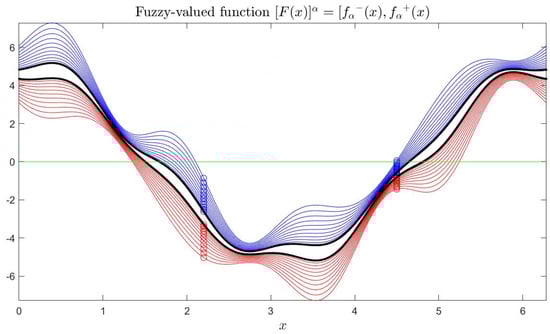
Figure 1. Level-wise endpoint graphical representation of the fuzzy-valued function defined by (39) and (40). In this representation, the core, highlighted by the black curves, is the interval-valued function $x⟶[f_1^{-}\left(x\right),f_1^{+}\left(x\right)]$, while the other $\alpha$-cuts are represented by red-colored curves for the left extreme functions $f_{\alpha }^{-}\left(x\right)$ and blue-colored curves for the right extreme functions $f_{\alpha }^{+}\left(x\right)$. The two marked points correspond to x = 2.2 and x = 4.5.

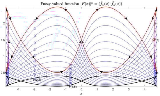
Figure 2. Level-wise midpoint graphical representation in the half plane $(\widehat{z};\tilde{z})$ for the same example defined by (39) and (40). In this figure, each curve represents a single $\alpha$-cut. The core is depicted by the black curve, while the support is shown by the red curve. The arrows give the direction of x from initial 0 to final $2\pi$.

In Figure 3, based on the midpoint representation, we obtain that the red lines on the right pictures reconstruct the eleven $\alpha$-cuts and it is established that y and $\widehat{z}$ share the same domain, and the linear vertical segment in the midpoint representation corresponds to a symmetric membership function having the same value of ${\widehat{f}}_{\alpha }\left(x\right)$ for all $\alpha$.

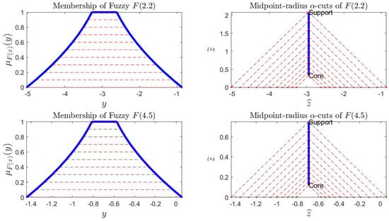
Figure 3. Membership function and level-wise midpoint representations of values $F(2;2)$ and $F(4;5)$ of the fuzzy-valued function $F\left(x\right)$ described in Figure 1. In the midpoint representation, a vertical curve depicts the shift of the computed $\alpha$-cuts for $n=11$. The red lines in the images on the right illustrate the reconstruction of these $\alpha$-cuts. It is important to note that y and $\widehat{z}$ denote the same domain, and that a straight vertical segment in the midpoint representation corresponds to a symmetric membership function with a constant value of ${\widehat{f}}_{\alpha }\left(x\right)$ across all levels of $\alpha$.

Definition 9.

Let $F:[a,b]\to {\mathbb{R}}_{\mathit{F}}$ be a fuzzy function, where ${\left[F\left(x\right)\right]}_{\alpha }=\left({\widehat{f}}_{\alpha }\left(x\right);{\tilde{f}}_{\alpha }\left(x\right)\right)$ for all $\alpha \in [0,1]$. We say that F is

(a-i) $(⪷)$-nondecreasing on $[a,b]$ if $x_1<x_2$ implies $F\left(x_1\right)⪷F\left(x_2\right)$ for all $x_1,x_2\in [a,b]$;

(a-ii) $(⪷)$-nonincreasing on $[a,b]$ if $x_1<x_2$ implies $F\left(x_2\right)⪷F\left(x_1\right)$ for all $x_1,x_2\in [a,b]$;

(b-i) (strictly) $(\precsim )$-increasing on $[a,b]$ if $x_1<x_2$ implies $F\left(x_1\right)\precsim F\left(x_2\right)$ for all $x_1,x_2\in [a,b]$;

(b-ii) (strictly) $(\precsim )$-decreasing on $[a,b]$ if $x_1<x_2$ implies $F\left(x_2\right)\precsim F\left(x_1\right)$ for all $x_1,x_2\in [a,b]$;

(c-i) (strongly) $(\prec )$-increasing on $[a,b]$ if $x_1<x_2$ implies $F\left(x_1\right)\prec F\left(x_2\right)$ for all $x_1,x_2\in [a,b]$;

(c-ii) (strongly) $(\prec )$-decreasing on $[a,b]$ if $x_1<x_2$ implies $F\left(x_2\right)\prec F\left(x_1\right)$ for all $x_1,x_2\in [a,b]$.

If one of the six conditions is satisfied, we say that F is monotonic on $[a,b]$; the monotonicity is strict if (b-i,b-ii) or strong if (c-i,c-ii) are satisfied.

We can also analyze the monotonicity of $F:[a,b]\to {\mathbb{R}}_{\mathit{F}}$ locally, in a neighborhood of an interior point $x_0\in ]a,b[$, by considering condition $F\left(x\right)⪷F\left(x_0\right)$ (or condition $F\left(x\right)⪸F\left(x_0\right)$) for $x\in ]a,b[$ and $\left|x-x_0\right|<\delta$ with a positive small $\delta$.

Definition 10.

Let $F:[a,b]\to {\mathbb{R}}_{\mathit{F}}$ be a fuzzy function, where ${\left[F\left(x\right)\right]}_{\alpha }=\left({\widehat{f}}_{\alpha }\left(x\right);{\tilde{f}}_{\alpha }\left(x\right)\right)$ for all $\alpha \in [0,1]$ and $x_0\in ]a,b[$. Let $U_{\delta }\left(x_0\right)=\{x;\left|x-x_0\right|<\delta \}$ (for positive δ) denote a neighborhood of $x_0$. We say that F is (locally)

(a-i) $(⪷)$-nondecreasing at $x_0$ if $x_1<x_2$ implies $F\left(x_1\right)⪷F\left(x_2\right)$ for all $x_1,x_2\in U_{\delta }\left(x_0\right)\cap [a,b]$ and some $\delta >0$;

(a-ii) $(⪷)$-nonincreasing at $x_0$ if $x_1<x_2$ implies $F\left(x_2\right)⪷F\left(x_1\right)$ for all $x_1,x_2\in U_{\delta }\left(x_0\right)\cap [a,b]$ and some $\delta >0$;

(b-i) (strictly)$(\precsim )$-increasing at $x_0$ if $x_1<x_2$ implies $F\left(x_1\right)\precsim F\left(x_2\right)$ for all $x_1,x_2\in U_{\delta }\left(x_0\right)\cap [a,b]$ and some $\delta >0$;

(b-ii) (strictly)$(\precsim )$-decreasing at $x_0$ if $x_1<x_2$ implies $F\left(x_2\right)\precsim F\left(x_1\right)$ for all $x_1,x_2\in U_{\delta }\left(x_0\right)\cap [a,b]$ and some $\delta >0$;

(c-i) (strongly) $(\precsim )$-increasing at $x_0$ if $x_1<x_2$ implies $F\left(x_1\right)\prec F\left(x_2\right)$ for all $x_1,x_2\in U_{\delta }\left(x_0\right)\cap [a,b]$ and some $\delta >0$;

(c-ii) (strongly) $(\precsim )$-decreasing at $x_0$ if $x_1<x_2$ implies $F\left(x_2\right)\prec F\left(x_1\right)$ for all $x_1,x_2\in U_{\delta }\left(x_0\right)\cap [a,b]$ and some $\delta >0$.

Proposition 8.

Let $F:[a,b]\to {\mathbb{R}}_{\mathit{F}}$ be a fuzzy function, where $F_{\alpha }\left(x\right)=\left({\widehat{f}}_{\alpha }\left(x\right);{\tilde{f}}_{\alpha }\left(x\right)\right)$ for $\alpha \in [0,1]$ and $x_0\in ]a,b[$. Then

1.

$F\left(x\right)$ is $(⪷)$-nondecreasing at $x_0$ if and only if ${\widehat{f}}_{\alpha }\left(x\right)$ is nondecreasing, ${\tilde{f}}_{\alpha }\left(x\right)-{\widehat{f}}_{\alpha }\left(x\right)$ is nonincreasing and ${\tilde{f}}_{\alpha }\left(x\right)+{\widehat{f}}_{\alpha }\left(x\right)$ is nondecreasing at $x_0$ for all $\alpha \in [0,1]$;

2.

$F\left(x\right)$ is $(⪷)$-nonincreasing at $x_0$ if and only if ${\widehat{f}}_{\alpha }\left(x\right)$ is nonincreasing, ${\tilde{f}}_{\alpha }\left(x\right)-{\widehat{f}}_{\alpha }\left(x\right)$ is nondecreasing and ${\tilde{f}}_{\alpha }\left(x\right)+{\widehat{f}}_{\alpha }\left(x\right)$ is nonincreasing at $x_0$ for all $\alpha \in [0,1]$.

Analogous conditions are valid for strict and strong monotonicity.

Proposition 9.

Let $F:]a,b[\to {\mathbb{R}}_{\mathit{F}}$ be a fuzzy function, where ${\left[F\left(x\right)\right]}_{\alpha }=\left({\widehat{f}}_{\alpha }\left(x\right);{\tilde{f}}_{\alpha }\left(x\right)\right)$ for all $\alpha \in [0,1]$ and let F be LgH-differentiable at the internal points $x\in ]a,b[$. Then

1.

If F is $(⪷)$-nondecreasing on $]a,b[$, then for all x, $F_{LgH}^{\prime }\left(x\right)⪸0$;

2.

If F is $(⪷)$-nonincreasing on $]a,b[$, then for all x, $F_{LgH}^{\prime }\left(x\right)⪷0$.

A similar result is obtained immediately by relating the strong (local) monotonicity of F to the “sign” of its left and right derivatives $F_{\left(l\right)LgH}^{\prime }\left(x\right)$ and $F_{\left(r\right)LgH}^{\prime }\left(x\right)$; note that at the extreme points of $[a,b]$, only the right monotonicity (in a) or left monotonicity (in b) and the right or left derivatives are considered.

Proposition 10.

Let $F:[a,b]\to {\mathbb{R}}_{\mathit{F}}$ be a fuzzy function, where ${\left[F\left(x\right)\right]}_{\alpha }=\left({\widehat{f}}_{\alpha }\left(x\right);{\tilde{f}}_{\alpha }\left(x\right)\right)$ for all $\alpha \in [0,1]$ with left and/or right gH-derivatives at a point $x_0\in [a,b]$. Then

(i.a) if $0\prec F_{\left(l\right)LgH}^{\prime }\left(x_0\right)$, then F is strongly $(\prec )$-increasing on $[x_0-\delta ,x_0]$ for some $\delta >0$ (here $x_0>a$);

(i.b) if $0\prec F_{\left(r\right)LgH}^{\prime }\left(x_0\right)$, then F is strongly $(\prec )$-increasing on $[x_0,x_0+\delta ]$ for some $\delta >0$ (here $x_0<b$);

(ii.a) if $0\succ F_{\left(l\right)LgH}^{\prime }\left(x_0\right)$, then F is strongly $(\prec )$-decreasing on $[x_0-\delta ,x_0]$ for some $\delta >0$ (here $x_0>a$);

(ii.b) if $0\succ F_{\left(r\right)LgH}^{\prime }\left(x_0\right)$, then F is strongly $(\prec )$-decreasing on $[x_0,x_0+\delta ]$ for some $\delta >0$ (here $x_0<b$).

As already performed for the monotonicity property, it is possible to manage the concavity and convexity of fuzzy-valued functions; in particular, there are three types of convexity.

Definition 11.

Let $F:[a,b]\to {\mathbb{R}}_{\mathit{F}}$ be a function and let ⪷ be a partial order on ${\mathbb{R}}_{\mathit{F}}$. We say that

(a-i)$F$ is (⪷)-convex on $[a,b]$ if and only if $F((1-\lambda )x_1+\lambda x_2)⪷(1-\lambda )F\left(x_1\right)+\lambda F\left(x_2\right),$ $\forall x_1,x_2\in [a,b]$ and all $\lambda \in [0,1]$;

(a-ii)$F$ is (${⪷}_{{\gamma }^{-},{\gamma }^{+}}$)-concave on $[a,b]$ if and only if $F((1-\lambda )x_1+\lambda x_2)⪸(1-\lambda )F\left(x_1\right)+\lambda F\left(x_2\right),$ $\forall x_1,x_2\in [a,b]$ and all $\lambda \in [0,1]$.

(b-i)$F$ is strictly (≾)-convex on $[a,b]$ if and only if $F((1-\lambda )x_1+\lambda x_2)\precsim (1-\lambda )F\left(x_1\right)+\lambda F\left(x_2\right),$ $\forall x_1,x_2\in [a,b]$ and all $\lambda \in ]0,1[$;

(b-ii)$F$ is strictly (≾)-concave on $[a,b]$ if and only if $F((1-\lambda )x_1+\lambda x_2)\succsim (1-\lambda )F\left(x_1\right)+\lambda F\left(x_2\right),$ $\forall x_1,x_2\in [a,b]$ and all $\lambda \in ]0,1[$.

(c-i)$F$ is strongly (≺)-convex on $[a,b]$ if and only if $F((1-\lambda )x_1+\lambda x_2)\prec (1-\lambda )F\left(x_1\right)+\lambda F\left(x_2\right),$ $\forall x_1,x_2\in [a,b]$ and all $\lambda \in ]0,1[$;

(c-ii)$F$ is strongly (≺)-concave on $[a,b]$ if and only if $F((1-\lambda )x_1+\lambda x_2)\succ (1-\lambda )F\left(x_1\right)+\lambda F\left(x_2\right),$ $\forall x_1,x_2\in [a,b]$ and all $\lambda \in ]0,1[$.

Concavity and convexity of a function ${\left[F\right]}_{\alpha }=\left({\widehat{f}}_{\alpha };{\tilde{f}}_{\alpha }\right)$ $\alpha \in [0,1]$ satisfy the property that F is (⪷)-concave if and only if $-F$ is (⪷)-convex.

Proposition 11.

Let $F:[a,b]\to {\mathbb{R}}_{\mathit{F}}$ with ${\left[F\right]}_{\alpha }=\left({\widehat{f}}_{\alpha };{\tilde{f}}_{\alpha }\right)$ for all $\alpha \in [0,1]$ and ⪷ be a given partial order; then

1.

F is (⪷)-convex if and only if ${\widehat{f}}_{\alpha }$ is convex, ${\tilde{f}}_{\alpha }+{\gamma }^{-}·{\widehat{f}}_{\alpha }$ is concave and ${\tilde{f}}_{\alpha }+{\gamma }^{+}·{\widehat{f}}_{\alpha }$ is convex;

2.

F is (⪷)-concave if and only if ${\widehat{f}}_{\alpha }$ is concave, ${\tilde{f}}_{\alpha }+{\gamma }^{-}·{\widehat{f}}_{\alpha }$ is convex and ${\tilde{f}}_{\alpha }+{\gamma }^{+}·{\widehat{f}}_{\alpha }$ is concave.

According to Proposition 11, it is easy to prove that F is (⪷)-convex (or concave) if and only if $f_{\alpha }^{-}$ and $f_{\alpha }^{+}$ are convex (or concave) for all $\alpha \in [0,1]$. Additionally, several ways to analyze (⪷)-convexity (or concavity) in terms of the first or second derivatives of functions ${\widehat{f}}_{\alpha }$, ${\widehat{f}}_{\alpha }-{\tilde{f}}_{\alpha }$ and ${\tilde{f}}_{\alpha }+{\widehat{f}}_{\alpha }$ can be easily derived.

Proposition 12.

Let $F:]a,b[\to {\mathbb{R}}_{\mathit{F}}$ with ${\left[F\right]}_{\alpha }=\left({\widehat{f}}_{\alpha };{\tilde{f}}_{\alpha }\right)$ for all $\alpha \in [0,1]$. Real-valued functions ${\widehat{f}}_{\alpha }$ and ${\tilde{f}}_{\alpha }$ are differentiable, then:

1. If the first order derivatives ${\widehat{f}}_{\alpha }^{\prime }$ and ${\tilde{f}}_{\alpha }^{\prime }$ exist, then:

(1-a) F is (⪷)-convex on $]a,b[$ if and only if ${\widehat{f}}_{\alpha }^{\prime }$, ${\widehat{f}}_{\alpha }^{\prime }-{\tilde{f}}_{\alpha }^{\prime }$ and ${\tilde{f}}_{\alpha }^{\prime }+{\widehat{f}}_{\alpha }^{\prime }$ are increasing (nondecreasing) for all $\alpha \in [0,1]$ on $]a,b[$;

(1-b) F is (⪷)-concave on $]a,b[$ if and only if ${\widehat{f}}_{\alpha }^{\prime }$, ${\widehat{f}}_{\alpha }^{\prime }-{\tilde{f}}_{\alpha }^{\prime }$ and ${\tilde{f}}_{\alpha }^{\prime }+{\widehat{f}}_{\alpha }^{\prime }$ are decreasing (nonincreasing) for all $\alpha \in [0,1]$ on $]a,b[$;

2. If the second order derivatives ${\widehat{f}}_{\alpha }^{″}$ and ${\tilde{f}}_{\alpha }^{″}$ exist and are continuous, then:

(2-a) F is (⪷)-convex on $]a,b[$ if and only if ${\widehat{f}}_{\alpha }^{″}\ge 0$, ${\widehat{f}}_{\alpha }^{″}-{\tilde{f}}_{\alpha }^{″}\ge 0$ and ${\tilde{f}}_{\alpha }^{″}+{\widehat{f}}_{\alpha }^{″}\ge 0$ for all $\alpha \in [0,1]$ on $]a,b[$;

(2-b) F is (⪷)-concave on $]a,b[$ if and only if ${\widehat{f}}_{\alpha }^{″}\le 0$, ${\widehat{f}}_{\alpha }^{″}-{\tilde{f}}_{\alpha }^{″}\le 0$ and ${\tilde{f}}_{\alpha }^{″}+{\widehat{f}}_{\alpha }^{″}\le 0$ for all $\alpha \in [0,1]$ on $]a,b[$.

Remark 1.

Similarly to the relationship between the convexity for ordinary functions and the sign of the second derivative, we can establish conditions for convexity of fuzzy functions and the sign of the second-order LgH-derivative $F_{LgH}^{″}\left(x\right)$; for example, a sufficient condition for strong ≺-convexity is the following (compare with Proposition 12):

1.

If $F_{LgH}^{″}\left(x_0\right)\prec 0$ then $F\left(x\right)$ is strongly concave at $x_0$.

2.

If $F_{LgH}^{″}\left(x_0\right)\succ 0$ then $F\left(x\right)$ is strongly convex at $x_0$.

The periodicity property for fuzzy-valued functions can also be defined.

Definition 12.

A function $F:[a,b]\to {\mathbb{R}}_{\mathit{F}}$ is said to be periodic if, for some nonzero constant $T\in ]0,b-a[$, it occurs that $F(x+T)=F\left(x\right)$ for all $x\in [a,b]$ with $x+T\in [a,b]$ (i.e., for all $x\in [a,b-T]$). A nonzero constant T for which this is verified is called a period of the function and if there exists a least positive constant T with this property, it is called the fundamental period.

Clearly, in case F has a period T, this also implies that $F_{\alpha }$ for all $\alpha \in [0,1]$ has a period T, i.e., for all $\alpha \in [0,1]$, ${\widehat{f}}_{\alpha }$ and ${\tilde{f}}_{\alpha }$ are periodic with period T. On the other side, the periodicity of F is not necessarily implied by the periodicity of the functions $F_{\alpha }$ for all $\alpha \in [0,1]$.

Proposition 13.

Let $F:[a,b]\to {\mathbb{R}}_{\mathit{F}}$ be a continuous function such that ${\left[F\left(x\right)\right]}_{\alpha }=({\widehat{f}}_{\alpha }\left(x\right);{\tilde{f}}_{\alpha }\left(x\right))$ for all $\alpha \in [0,1]$ with ${\widehat{f}}_{\alpha }$ periodic of period $\widehat{T}$ and ${\tilde{f}}_{\alpha }$ of period $\tilde{T}$. Then it holds that:

(1) 

if the periods $\widehat{T}$ and $\tilde{T}$ are commensurable, i.e., ${\displaystyle \frac{\widehat{T}}{\tilde{T}}}\in \mathbb{Q}$ (${\displaystyle \frac{\widehat{T}}{\tilde{T}}}={\displaystyle \frac{p}{q}}$, such that p and q are coprime) then the function F is periodic of period $T=lcm(\widehat{T},\tilde{T})$, i.e, T is the least common multiple between $\widehat{T}$ and $\tilde{T}$ (i.e., $T=p\tilde{T}=q\widehat{T}$);

(2) 

if the periods $\widehat{T}$ and $\tilde{T}$ are not commensurable, i.e., ${\displaystyle \frac{\widehat{T}}{\tilde{T}}}\notin \mathbb{Q}$, then function F is not periodic.

The function depicted in all the preceding figures, defined by (39) and (40), provides a clear example of a periodic function with period p = 2π.

5. Extrema of Fuzzy Valued Functions

The concepts of simple, strict and strong monotonicity defined above, based on the orders ⪷, ≾ and ≺, give rise to different concepts of extrema.

Regarding the demonstrations of the results presented below, reference is made to those discussed in [6], as the procedures and steps are similar for each $\alpha \in [0,1]$; therefore, the results are provided here without further demonstrations. Additionally, the following terminology will be adopted.

Definition 13.

If $F\left(x_0\right)⪷F\left(x\right)$, we say that $F\left(x_0\right)$ dominates $F\left(x\right)$ with respect to the partial order ⪷ (for short, $F\left(x_0\right)$ $(⪷)$-dominated $F\left(x\right)$), or equivalently that $F\left(x\right)$ is $(⪷)$-dominated by $F\left(x_0\right)$. We say that $F\left(x\right)$ and $F\left(x_0\right)$ are incomparable with respect to ⪷ if both $F\left(x_0\right)⪷F\left(x\right)$ and $F\left(x\right)⪷F\left(x_0\right)$ are not valid. Analogous domination rules are defined in terms of the strict and strong order relations ≾ and ≺, respectively.

Now the basic concepts of order-based minimum and maximum points can be introduced for fuzzy-valued functions.

Definition 14.

Let $F:[a,b]\to {\mathbb{R}}_{\mathit{F}}$ be a fuzzy-valued function and $x_0\in [a,b]$. We say that, with respect to ⪷,

(a) 

$x_0$ is a local lattice-minimum point of F ($min$-point for short) if there exists $\delta >0$ such that $F\left(x_0\right)⪷F\left(x\right)$ for all $x\in ]x_0-\delta ,x_0+\delta [\cap [a,b]$, i.e., if all $F\left(x\right)$ around $x_0$ are $(⪷)$-dominated by $F\left(x_0\right)$;

(b) 

$x_0$ is a local lattice-maximum point of F ($max$-point for short) if there exists $\delta >0$ such that $F\left(x\right)⪷F\left(x_0\right)$ for all $x\in ]x_0-\delta ,x_0+\delta [\cap [a,b]$, i.e., if all $F\left(x\right)$ around $x_0$ $(⪷)$-dominate $F\left(x_0\right)$.

It will be helpful to explicitly establish the conditions for $(⪷)$-dominance of a general fuzzy function $F\left(x\right)$, with respect to fuzzy functions $F\left(x_m\right)$ and $F\left(x_M\right)$, that characterize the minimality and the maximality of a point $x_m$ (for min) or a point $x_M$ (for max). Avoiding making an explicit distinction between strict or strong dominance, we have, for all $\alpha \in [0,1]$:

$$F\left(x\right)⪸F\left(x_m\right)\iff \left\{\begin{array}{c}{\widehat{f}}_{\alpha }\left(x\right)\ge {\widehat{f}}_{\alpha }\left(x_m\right)\\ {\tilde{f}}_{\alpha }\left(x\right)\le {\tilde{f}}_{\alpha }\left(x_m\right)+\left({\widehat{f}}_{\alpha }\left(x\right)-{\widehat{f}}_{\alpha }\left(x_m\right)\right)\\ {\tilde{f}}_{\alpha }\left(x\right)\ge {\tilde{f}}_{\alpha }\left(x_m\right)-\left({\widehat{f}}_{\alpha }\left(x\right)-{\widehat{f}}_{\alpha }\left(x_m\right)\right),\end{array}\right.$$

(41)

and

$$F\left(x\right)⪷F\left(x_M\right)\iff \left\{\begin{array}{c}{\widehat{f}}_{\alpha }\left(x\right)\le {\widehat{f}}_{\alpha }\left(x_M\right)\\ {\tilde{f}}_{\alpha }\left(x\right)\ge {\tilde{f}}_{\alpha }\left(x_M\right)+\left({\widehat{f}}_{\alpha }\left(x\right)-{\widehat{f}}_{\alpha }\left(x_M\right)\right)\\ {\tilde{f}}_{\alpha }\left(x\right)\le {\tilde{f}}_{\alpha }\left(x_M\right)-\left({\widehat{f}}_{\alpha }\left(x\right)-{\widehat{f}}_{\alpha }\left(x_M\right)\right).\end{array}\right.$$

(42)

With the following proposition it is possible to show that lattice-type minimality and maximality, with respect to the partial order ⪷, can be identified exactly in terms of functions $f_{\alpha }^{-}$ and $f_{\alpha }^{+}$, for all $\alpha \in [0,1]$, as follows.

Proposition 14.

Let $F:[a,b]\to {\mathbb{R}}_{\mathit{F}}$ be a fuzzy-valued function, where ${\left[F\left(x\right)\right]}_{\alpha }=[f_{\alpha }^{-}\left(x\right),f_{\alpha }^{+}\left(x\right)]$ for all $\alpha \in [0,1]$. Then

(a) 

$x_m\in [a,b]$ is a min-point of F if and only if it is a minimum of functions $f_{\alpha }^{-}$ and $f_{\alpha }^{+}$ for all $\alpha \in [0,1]$;

(b) 

$x_M\in [a,b]$ is a max-point of F if and only if it is a maximum of functions $f_{\alpha }^{-}$ and $f_{\alpha }^{+}$ for all $\alpha \in [0,1]$.

What has been seen above shows the restricting notion of a lattice-extreme point, since it is rare for simultaneous extrema to occur for the two functions $f_{\alpha }^{-}$ and $f_{\alpha }^{+}$. Taking into account the possibility that the fuzzy functions $F\left(x\right)$ for different x are locally incomparable with respect to the actual order relation, the following definition is more general.

Definition 15.

Let $F:[a,b]\to {\mathbb{R}}_{\mathit{F}}$ be a fuzzy-valued function and $x_m,x_M\in [a,b]$. We say that, with respect to the order ⪷ and the corresponding strict order ≾,

(c) $x_m$ is a local best-minimum point of F (best-min for short) if:

(c.1) it is a local minimum for the midpoint function ${\widehat{f}}_{\alpha }$ for all $\alpha \in [0,1]$, and

(c.2) there exists $\delta >0$ and no point $x\in ]x_m-\delta ,x_m+\delta [\cap [a,b]$ with $F\left(x\right)\ne F\left(x_m\right)$ such that $F\left(x\right)⪷F\left(x_m\right)$;

(d) $x_M$ is a local best-maximum point of F (best-max for short) if:

(d.1) it is a local maximum for the midpoint function ${\widehat{f}}_{\alpha }$ for all $\alpha \in [0,1]$, and

(d.2) there exists $\delta >0$ and no point $x\in ]x_M-\delta ,x_M+\delta [\cap [a,b]$ with $F\left(x\right)\ne F\left(x_M\right)$ such that $F\left(x_M\right)⪷F\left(x\right)$.

We can give the definitions of strict and strong (local) extremal points considering the strict ≾ or the strong ≺ orders associated to the lattice order ⪷.

Definition 16.

Let $F:[a,b]\to {\mathbb{R}}_{\mathit{F}}$ be a fuzzy-valued function. With respect to an order ⪷ and the associated strict order ≾ or strong order ≺, we say that

-

a best-min point $x_m$ is a strict (respectively, strong) best-minimum point if there exists $\delta >0$ and no point $x\in ]x_m-\delta ,x_m+\delta [\cap [a,b]$ with $F\left(x\right)\precsim F\left(x_m\right)$ (or $F\left(x\right)\prec F\left(x_m\right)$, respectively);

-

a best-max point $x_M$ is a strict (respectively, strong) best-maximum point if there exists $\delta >0$ and no point $x\in ]x_M-\delta ,x_M+\delta [\cap [a,b]$ with $F\left(x_M\right)\precsim F\left(x\right)$ (or $F\left(x_M\right)\prec F\left(x\right)$, respectively).

Considering the case in which $x_m\in [a,b]$ is a lattice-minimum point, that is, there exists a neighborhood of $x_m$ such that all $F\left(x\right)$ satisfy (41), we have that no such $F\left(x\right)$ is incomparable with $F\left(x_m\right)$; similarly, if $x_M\in [a,b]$ is a lattice-maximum point, i.e., there exists a neighborhood of $x_M$ such that all $F\left(x\right)$ satisfy (42), then no such $F\left(x\right)$ is incomparable with $F\left(x_M\right)$. This fact can be expressed by saying that the (local) min-efficient frontier for the $min$-point $x_m$ is concentrated into the fuzzy function $F\left(x_m\right)$; analogously, the (local) max-efficient frontier for the max-point $x_M$ is concentrated into the fuzzy function $F\left(x_M\right)$.

On the other hand, in the case where $x_m$ and $x_M$ are best-type and not lattice-type extrema, then it is fundamental to identify the fuzzy function $F\left(x\right)$, in particular with x in a neighborhood of $x_m$ or $x_M$, that are not min-dominated by $F\left(x_m\right)$ (or do not max-dominate $F\left(x_M\right)$); clearly, these $F\left(x\right)$ are necessarily (⪷)-incomparable with $F\left(x_m\right)$ (or with $F\left(x_M\right)$, respectively).

Therefore, corresponding to a minimum and to a maximum point of F, we are interested in identifying the locally (min/max)-efficient fuzzy function $F\left(x\right)$ and what we will call the local min or max efficient frontier for $F\left(x_m\right)$ and $F\left(x_M\right)$ around points $x_m$ and $x_M$, respectively.

In order to find the efficient frontier for a strict minimum and a strict maximum, the first thing to do is the following:

Proposition 15.

Let $F:[a,b]\to {\mathbb{R}}_{\mathit{F}}$ be a fuzzy-valued function. Let $x_m,x_M\in [a,b]$ be local strict best-min and local strict best-max points of F. Then, there exist $x_m^L\le x_m$, $x_m^R\ge x_m$, $x_M^L\le x_M$ and $x_M^R\ge x_M$ (all belonging to $[a,b]$) such that, respectively,

1.

$F\left(x\right)$ is incomparable with $F\left(x_m\right)$, for all $x\in [x_m^L,x_m^R]$, $x\ne x_m$;

2.

$F\left(x\right)$ is incomparable with $F\left(x_M\right)$, for all $x\in [x_M^L,x_M^R]$, $x\ne x_M$.

A significant consequence of Proposition 15 is a sufficient condition for a lattice type external point.

Proposition 16.

Let $F:[a,b]\to {\mathbb{R}}_{\mathit{F}}$; if $x_m$ (respectively, $x_M$) is a minimum point (a maximum point) of function ${\widehat{f}}_{\alpha }\left(x\right)$ for all $\alpha \in [0,1]$ and $x_m^L=x_m=x_m^R$ (or $x_M^L=x_M=x_M^R$) then $x_m$ is a lattice min-point (respectively $x_M$ is a lattice max-point) of $F\left(x\right)$ and vice versa.

Another crucial consequence of the last proposition is that the efficient function $F\left(x\right)$, relative to the best minimum point $x_m$ or to the best maximum point $x_M$, considering the case where they are not extremal points of the lattice, must be sought between the points $x\in [x_m^L,x_m^R]$ and $x\in [x_M^L,x_M^R]$, respectively.

The last step is to feature the points of $[x_m^L,x_m^R]$ and $[x_M^L,x_M^R]$ that contain, respectively, $x_m$, $x_M$ and are such that all corresponding $F\left(x\right)$ define the local efficient frontier of F around $F\left(x_m\right)$ and $F\left(x_M\right)$.

We begin by providing a formal definition of the min/max efficient frontier:

Definition 17.

Let $F:[a,b]\to {\mathbb{R}}_{\mathit{F}}$ be a fuzzy-valued function and let $x_m,x_M\in [a,b]$ be local strict best-min and local strict best-max points of F with respect to the partial order ⪷.

(a) The (local) min-efficient frontier of function F associated to the best-min point $x_m$ (or to the best-min fuzzy-value $F\left(x_m\right)$) is the set $E_{\min }(F,x_m)$ of fuzzy-values $F\left(x\right)$ such that:

(a.1) $F\left(x_m\right)\in E_{\min }(F,x_m)$,

(a.2) if $x^{\prime },x^{″}\in [a,b]$ and $F\left(x^{\prime }\right),F\left(x^{″}\right)\in E_{\min }(F,x_m)$ then $F\left(x^{\prime }\right)$ and $F\left(x^{″}\right)$ are (⪷)-incomparable,

(a.3) no other set $E^{\prime }$ containing $E_{\min }(F,x_m)$ has property (a.2). The set of points $x\in [x_m^L,x_m^R]$ such that $F\left(x\right)\in E_{\min }(F,x_m)$ are the local min-efficient points corresponding to $x_m$ and is denoted by $ef{f}_{\min }(F;x_m)$.

(b) The (local) max-efficient frontier of function F associated to the best-max point $x_M$ (or to the best-max fuzzy-value $F\left(x_M\right)$) is the set $E_{\max }(F,x_M)$ of fuzzy-values $F\left(x\right)$ such that:

(b.1) $F\left(x_M\right)\in E_{\max }(F,x_M)$,

(b.2) if $x^{\prime },x^{″}\in [a,b]$ and $F\left(x^{\prime }\right),F\left(x^{″}\right)\in E_{\max }(F,x_M)$ then $F\left(x^{\prime }\right)$ and $F\left(x^{″}\right)$ are (⪷)-incomparable,

(b.3) no other set $E^{\prime }$ containing $E_{\max }(F,x_m)$ has property (b.2). The set of points $x\in [x_M^L,x_M^R]$ such that $F\left(x\right)\in E_{\max }(F,x_M)$ are the local max-efficient points corresponding to $x_M$ and is denoted by $ef{f}_{\max }(F;x_M)$.

The efficient frontiers $ef{f}_{\min }(F;x_m)$ or $ef{f}_{\max }(F;x_M)$ are obviously subsets of the interval in Proposition 15; but, in cases where the function $F\left(x\right)$ has possible inflection or angular points, tangencies of high order, multiple nodes, fractal-like or complex pathological patterns, their characterization is not at all simple.

Let us consider the curve $C_F$, in the half-plane $(\widehat{z};\tilde{z})$ with parametric equations $\widehat{z}={\widehat{f}}_{\alpha }\left(x\right)$, $\tilde{z}={\tilde{f}}_{\alpha }\left(x\right)$ and parameter $x\in [a,b]$ and assume that the curve is simple (without multiple points) and differentiable (i.e., both ${\widehat{f}}_{\alpha }\left(x\right)$ and ${\tilde{f}}_{\alpha }\left(x\right)$ have derivatives at internal points); we say that $C_F$ has the convexity property if, for each of its points, the curve lies on one side of the tangent line to it. In our case, the convexity of $C_F$ is only needed locally, considering the restriction of $F\left(x\right)$ to points around $x_m$ (or $x_M$). In particular, we fix the notion of local convexity of $C_F$ by distinguishing the case of a minimum to the case of a maximum point.

Taking into account specific assumptions about the function’s shape, the following results can be proven:

Proposition 17.

Let ⪷ be a partial order on ${\mathbb{R}}_{\mathit{F}}$ and let $F:[a,b]\to {\mathbb{R}}_{\mathit{F}}$ be a fuzzy-valued function with ${\left[F\left(x\right)\right]}_{\alpha }=[f_{\alpha }^{-}\left(x\right),f_{\alpha }^{+}\left(x\right)]$ for all $\alpha \in [0,1]$ such that $x_m\in ]a,b[$ is a local min point of ${\widehat{f}}_{\alpha }\left(x\right)$ for all $\alpha \in [0,1]$ and Assumption 1 is satisfied. Then there exist two points $x_m^{\prime },x_m^{″}\in [x_m^L,x_m^R]$ with $x_m^{\prime }\le x_m\le x_m^{″}$ and such that, for $x\in \left[x_m-{\delta }_m^{\prime },x_m+{\delta }_m^{″}\right]$,

(1) 

either $x_m^{\prime }$ maximizes ${\tilde{f}}_{\alpha }\left(x\right)-{\widehat{f}}_{\alpha }\left(x\right)$ and $x_m^{″}$ minimizes ${\tilde{f}}_{\alpha }\left(x\right)+{\widehat{f}}_{\alpha }\left(x\right)$ for all $\alpha \in [0,1]$,

(2) 

or $x_m^{\prime }$ minimizes ${\tilde{f}}_{\alpha }\left(x\right)+{\widehat{f}}_{\alpha }\left(x\right)$ and $x_m^{″}$ maximizes ${\tilde{f}}_{\alpha }\left(x\right)-{\widehat{f}}_{\alpha }\left(x\right)$ for all $\alpha \in [0,1]$,

and equivalently,

(i) 

either $x_m^{\prime }$ minimizes $f_{\alpha }^{-}\left(x\right)$ and $x_m^{″}$ minimizes $f_{\alpha }^{+}\left(x\right)$ for all $\alpha \in [0,1]$,

(ii) 

or $x_m^{\prime }$ maximizes $f_{\alpha }^{+}\left(x\right)$ and $x_m^{″}$ minimizes $f_{\alpha }^{-}\left(x\right)$ for all $\alpha \in [0,1]$.

Furthermore, interval $[x_m^{\prime },x_m^{″}]$ is the local efficient frontier $ef{f}_{min}(F;x_m)$ of Definition 17. In particular, if $x_m^{\prime }$ and $x_m^{″}$ are internal to the local convexity region and ${\widehat{f}}_{\alpha }\left(x\right)$, ${\tilde{f}}_{\alpha }\left(x\right)$ are differentiable at x for all $\alpha \in [0,1]$, then

$$\left\{\begin{array}{c}{\tilde{f}}_{\alpha }^{\prime }\left(x_m^{\prime }\right)={\widehat{f}}_{\alpha }^{\prime }\left(x_m^{\prime }\right)\\ {\tilde{f}}_{\alpha }^{\prime }\left(x_m^{″}\right)=-{\widehat{f}}_{\alpha }^{\prime }\left(x_m^{″}\right)\end{array}\right.\mathrm{or}\left\{\begin{array}{c}{\tilde{f}}_{\alpha }^{\prime }\left(x_m^{″}\right)={\widehat{f}}_{\alpha }^{\prime }\left(x_m^{″}\right)\\ {\tilde{f}}_{\alpha }^{\prime }\left(x_m^{\prime }\right)=-{\widehat{f}}_{\alpha }^{\prime }\left(x_m^{\prime }\right)\end{array}\right..$$

(43)

Proposition 18.

Let ⪷ be a partial order on ${\mathbb{R}}_{\mathit{F}}$ and let $F:[a,b]\to {\mathbb{R}}_{\mathit{F}}$ be fuzzy-valued function with ${\left[F\left(x\right)\right]}_{\alpha }=[f_{\alpha }^{-}\left(x\right),f_{\alpha }^{+}\left(x\right)]$ for all $\alpha \in [0,1]$ such that $x_M\in ]a,b[$ is a local max point of ${\widehat{f}}_{\alpha }\left(x\right)$ for all $\alpha \in [0,1]$ and Assumption 2 is satisfied. Then there exist two points $x_M^{\prime },x_M^{″}\in [x_M^L,x_M^R]$ with $x_M^{\prime }\le x_M\le x_M^{″}$ and such that, for $x\in \left[x_M-{\delta }_M^{\prime },x_M+{\delta }_M^{″}\right]$,

(1) 

either $x_M^{\prime }$ minimizes ${\tilde{f}}_{\alpha }\left(x\right)-{\widehat{f}}_{\alpha }\left(x\right)$ and $x_M^{″}$ maximizes ${\tilde{f}}_{\alpha }\left(x\right)+{\widehat{f}}_{\alpha }\left(x\right)$ for all $\alpha \in [0,1]$,

(2) 

or $x_M^{\prime }$ maximizes ${\tilde{f}}_{\alpha }\left(x\right)+{\widehat{f}}_{\alpha }\left(x\right)$ and $x_M^{″}$ minimizes ${\tilde{f}}_{\alpha }\left(x\right)-{\widehat{f}}_{\alpha }\left(x\right)$ for all $\alpha \in [0,1]$.

Equivalently,

(i) 

either $x_M^{\prime }$ maximizes $f_{\alpha }^{-}\left(x\right)$ and $x_M^{″}$ maximizes $f_{\alpha }^{+}\left(x\right)$, for all $\alpha \in [0,1]$,

(ii) 

or $x_M^{\prime }$ maximizes $f_{\alpha }^{+}\left(x\right)$ and $x_M^{″}$ maximizes $f_{\alpha }^{+}\left(x\right)$ for all $\alpha \in [0,1]$. Furthermore, interval $[x_M^{\prime },x_M^{″}]$ is the local efficient frontier $ef{f}_{max}(F;x_M)$ of Definition 17. In particular, if $x_M^{\prime }$ and $x_M^{″}$ are internal to the local convexity region and ${\widehat{f}}_{\alpha }\left(x\right)$, ${\tilde{f}}_{\alpha }\left(x\right)$ are differentiable at x for all $\alpha \in [0,1]$, then

$$\left\{\begin{array}{c}{\tilde{f}}_{\alpha }^{\prime }\left(x_M^{\prime }\right)={\widehat{f}}_{\alpha }^{\prime }\left(x_M^{\prime }\right)\\ {\tilde{f}}_{\alpha }^{\prime }\left(x_M^{″}\right)=-{\widehat{f}}_{\alpha }^{\prime }\left(x_M^{″}\right)\end{array}\right.\mathrm{or}\left\{\begin{array}{c}{\tilde{f}}_{\alpha }^{\prime }\left(x_M^{″}\right)={\widehat{f}}_{\alpha }^{\prime }\left(x_M^{″}\right)\\ {\tilde{f}}_{\alpha }^{\prime }\left(x_M^{\prime }\right)=-{\widehat{f}}_{\alpha }^{\prime }\left(x_M^{\prime }\right)\end{array}\right..$$

(44)

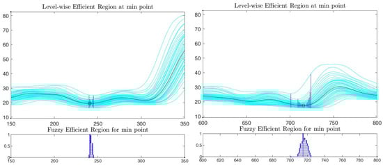
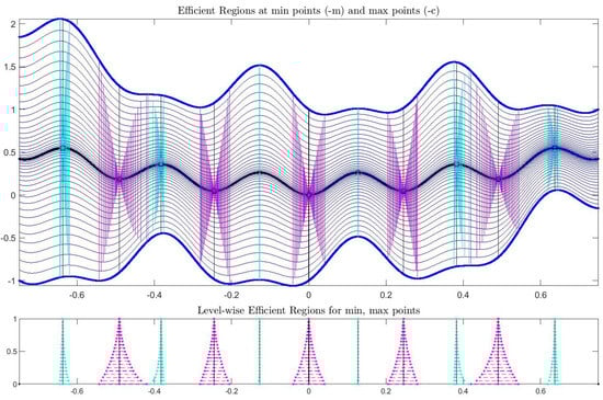
Developing the same examples (39) and (40), Figure 4 and Figure 5 show the Efficient Regions at two specific minimum and maximum points (both level-wise and fuzzy cases are indicated).

Figure 4. Level-wise efficient frontiers for specific max points of F(x) in examples defined by (39) and (40). The efficient frontiers are delimited by vertical red segments containing the max points. The corresponding Fuzzy Efficient Regions are displayed in the bottom part.

Figure 5. Level-wise efficient frontiers for specific min points of F(x) in examples defined by (39) and (40). The efficient frontiers are delimited by vertical red segments containing the max points. The corresponding Fuzzy Efficient Regions are displayed in the bottom part.

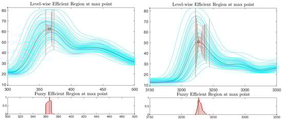
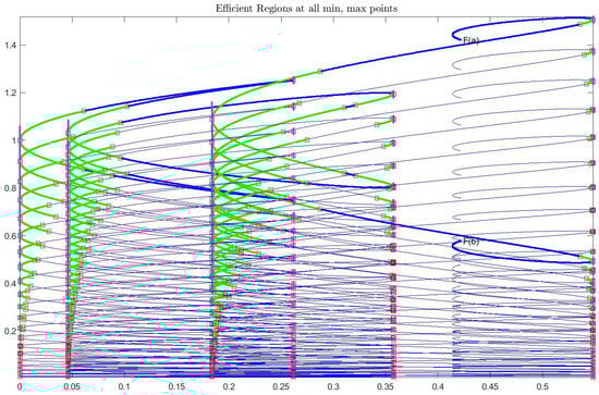
More generally, Figure 6 and Figure 7 summarize the efficient regions for all maximum and minimum points.

Figure 6. Efficient regions at all maximum and minimum points of F(x) in examples defined by (39) and (40). The respective level-wise efficient regions are shown below.

Figure 7. Function F(x) in examples (39) and (40) represented in midpoint form with all maximum and minimum points marked together with corresponding efficient regions.

The last part of the section is devoted to an attempt to see how the property of local extreme for a point $x_m$ (minimum) or $x_M$ (maximum) is connected to the left and/or right LgH-derivatives or to the LgH-derivative $F_{LgH}^{\prime }\left(x_0\right)$ when they assume the same value. To reach the goal, we introduce the following Fermat-like property:

Proposition 19.

Let $F:]a,b[\to {\mathbb{R}}_{\mathit{F}}$ be LgH-differentiable at $x_0\in ]a,b[$ and ⪷ be a partial order on ${\mathbb{R}}_{\mathit{F}}$. If $x_0$ is a lattice extremum for F (a lattice-min or a lattice-max point), then $F_{LgH}^{\prime }\left(x_0\right)=0$.

Proposition 20.

Let $F:[a,b]\to {\mathbb{R}}_{\mathit{F}}$, $x_0\in [a,b]$ and ⪷ be a partial order on ${\mathbb{R}}_{\mathit{F}}$. Suppose that F has left and right LgH-derivatives at $x_0$ (if $x_0=a$ or $x_0=b$, we consider only the right or the left LgH-derivatives, respectively):

(1.a) 

If $x_0$ is a lattice minimum point for F, then $F_{\left(l\right)LgH}^{\prime }\left(x_0\right)⪸0$ and $F_{\left(r\right)LgH}^{\prime }\left(x_0\right)⪷0$;

(1.b) 

If $x_0$ is a lattice maximum point for F, then $F_{\left(l\right)LgH}^{\prime }\left(x_0\right)⪷0$ and $F_{\left(r\right)LgH}^{\prime }\left(x_0\right)⪸0$.

Proposition 21.

Let $F:]a,b[\to {\mathbb{R}}_{\mathit{F}}$ be LgH-differentiable at $x_0\in ]a,b[$ and ${⪷}_{\alpha }$ be a partial order on ${\mathbb{R}}_{\mathit{F}}$.

(i) 

If $x_0$ is a best-minimum point for F, then $0\in$ $F_{LgH}^{\prime }\left(x_0\right)$.

(ii) 

If $x_0$ is a best-maximum point for F, then $0\in$ $F_{LgH}^{\prime }\left(x_0\right)$.

Notation: It is trivial to note that Proposition 21 is not valid for ⪷ of partial order on ${\mathbb{R}}_{\mathit{F}}$.

Analogously to the well-known situation for single-valued functions, the following are sufficient conditions based on the “sign” of the left and right LgH-derivatives.

Proposition 22.

Let $F:[a,b]\to {\mathbb{R}}_{\mathit{F}}$, $x_0\in [a,b]$ and ⪷ be a partial order on ${\mathbb{R}}_{\mathit{F}}$ and $\alpha \in [0,1]$. Suppose that F has left and right LgH-derivatives at $x_0$ (if $x_0=a$ or $x_0=b$ we consider only the right or the left LgH-derivatives, respectively):

(a) 

If $F_{\left(l\right)LgH}^{\prime }\left(x_0\right)\prec 0$ and $F_{\left(r\right)LgH}^{\prime }\left(x_0\right)\succ 0$, then $x_0$ is a best minimum point for F;

(b) 

If $F_{\left(l\right)LgH}^{\prime }\left(x_0\right)\succ 0$ and $F_{\left(r\right)LgH}^{\prime }\left(x_0\right)\prec 0$, then $x_0$ is a best maximum point for F.

Finally, it is possible to argue that the sign of the left and right LgH-derivatives established conditions for local extremes.

6. Conclusions and Further Work

Within the present paper, we developed new results to define extremal points (local or global minimum or maximum), in terms of the general LU-partial order, providing a general approach which can be extended to other types of partial orders. Another possible promising extension regards the analysis of concavity and convexity properties of fuzzy valued functions, through first-order and second-order LgH-derivatives.

It is anticipated that this theory may find practical application in future research. In this regard, the spectrum of potential applications is broad and diverse (see, for example, [17], where the authors examine the complexities inherent in assessing the quality of river waters, a multifaceted process influenced by parameters associated with intrinsic uncertainties that can be effectively modeled through the application of fuzzy sets, subsequently proposing an effective classification system for water pollution). In addition to the conventional roles in optimization and decision making, such as those widely discussed in [18], a notably impacting area of application is the scheduling of cross-docking activities within manufacturing sectors introduced in [19] where uncertain parameters are modeled as triangular interval-valued fuzzy numbers and multi-objective mathematical programming problems are solved. Although the aim of this paper is to systematize the use of the midpoint representation by providing powerful general order rules, the results play a crucial role in all contexts where optimization allows the solution of real problems.

Finally, recent studies detailed in [20] extend the differentiability for Interval-Valued functions of multiple variables versus a general approach to Fréchet-type and Gateaux-type gH-differentiability based on midpoint representation, contributing to the opening of new research directions extended to fuzzy-valued function calculus.

References

- Guerra, M.L.; Stefanini, L. A comparison index for interval ordering based on generalized Hukuhara difference. Soft Comput. 2012, 16, 1931–1943. [Google Scholar] [CrossRef]
- Kaleva, O. The calculus of fuzzy valued functions. Appl. Math. Lett. 1990, 3, 55–59. [Google Scholar] [CrossRef]
- Stefanini, L.; Bede, B. Generalized Hukuhara differentiability of interval-valued functions and interval differential equations. Nonlinear Anal. 2009, 71, 1311–1328. [Google Scholar] [CrossRef]
- Zhengguang, X.; Changping, S. Moving pattern-based forecasting model of a class of complex dynamical systems. In Proceedings of the 2011 50th IEEE Conference on Decision and Control and European Control Conference, Orlando, FL, USA, 12–15 December 2011; pp. 4967–4972. [Google Scholar] [CrossRef]
- Stefanini, L.; Guerra, M.L.; Amicizia, B. Interval analysis and calculus for interval-valued functions of a single variable. Part I: Partial orders, gH-derivative, monotonicity. Axioms 2019, 8, 113. [Google Scholar] [CrossRef]
- Stefanini, L.; Sorini, L.; Amicizia, B. Interval analysis and calculus for interval-valued functions of a single variable. Part II: External points, convexity, periodicity. Axioms 2019, 8, 114. [Google Scholar] [CrossRef]
- Amicizia, B.; Guerra, M.L.; Shahidi, M.; Sorini, L.; Stefanini, L. Midpoint representation of fuzzy-valued functions and applications. In Proceedings of the 2020 IEEE International Conference on Fuzzy Systems (FUZZ-IEEE), Glasgow, UK, 19–24 July 2020. [Google Scholar] [CrossRef]
- Stefanini, L.; Sorini, L.; Shahidi, M. New results in the calculus of fuzzy-valued functions using mid-point representations. In Information Processing and Management of Uncertainty in Knowledge-Based Systems, Proceedings of the 18th International Conference, IPMU 2020, Lisbon, Portugal, 15–19 June 2020; Springer: Cham, Switzerland, 2020. [Google Scholar] [CrossRef]
- Bede, B.; Stefanini, L. Generalized differentiability of fuzzy-valued functions. Fuzzy Sets Syst. 2013, 230, 119–141. [Google Scholar] [CrossRef]
- Zadeh, L.A. Fuzzy Sets. Inf. Control. 1965, 8, 338–353. [Google Scholar] [CrossRef]
- Bede, B. Mathematics of Fuzzy Sets and Fuzzy Logic; Studies in Fuzziness and Soft Computing n. 295; Springer: Berlin/Heidelberg, Germany, 2013. [Google Scholar] [CrossRef]
- Sengupta, A.; Pal, T.K. Fuzzy Preference Ordering of Interval Numbers in Decision Problems; Studies in Fuzziness and Soft Computing (STUDFUZZ); Springer: Berlin/Heidelberg, Germany, 2009; Volume 238. [Google Scholar] [CrossRef]
- Amicizia, B. Recent and New Perspectives in Interval Analysis. Ph.D. Thesis, University of Urbino, Urbino, Italy, 2023. Available online: https://hdl.handle.net/11576/2725531 (accessed on 1 April 2025).
- Kosheleva, O.; Kreinovich, V.; Pham, U.H. Decision Making Under Interval Uncertainty Revisited. Asian J. Econ. Bank. 2020, 5, 79–85. [Google Scholar] [CrossRef]
- Alefeld, G.; Mayer, G. Interval analysis: Theory and applications. J. Comput. Appl. Math. 2000, 121, 421–464. [Google Scholar] [CrossRef]
- Moore, R.E.; Kearfott, R.B.; Cloud, J.M. Introduction to Interval Analysis; SIAM: Philadelphia, PA, USA, 2009. [Google Scholar] [CrossRef]
- Das, A.K.; Gupta, N.; Mahmood, T.; Tripathy, B.C.; Das, R.; Das, S. An innovative fuzzy multi-criteria decision making model for analyzing anthropogenic influences on urban river water quality. Iran J. Comput. Sci. 2025, 8, 103–124. [Google Scholar] [CrossRef]
- Das, A.K.; Granados, C. An Advanced Approach to Fuzzy Soft Group Decision-Making Using Weighted Average Ratings. SN Comput. Sci. 2021, 2, 471. [Google Scholar] [CrossRef]
- Rajabzadeh, M.; Mousavi, S.M. A new interval-valued fuzzy optimization model for truck scheduling in a multi-door cross-docking system by considering transshipment and flexible dock doors extra cost. J. Fuzzy Syst. 2023, 20, 63–84. [Google Scholar] [CrossRef]
- Stefanini, L.; Arana-Jiménez, M.; Sorini, L. Fréchet and Gateaux gH-differentiability for interval valued functions of multiple variables. Inf. Sci. 2025, 691, 121601. [Google Scholar] [CrossRef]
Disclaimer/Publisher’s Note: The statements, opinions and data contained in all publications are solely those of the individual author(s) and contributor(s) and not of MDPI and/or the editor(s). MDPI and/or the editor(s) disclaim responsibility for any injury to people or property resulting from any ideas, methods, instructions or products referred to in the content. |
© 2025 by the authors. Licensee MDPI, Basel, Switzerland. This article is an open access article distributed under the terms and conditions of the Creative Commons Attribution (CC BY) license (https://creativecommons.org/licenses/by/4.0/).