Abstract
Predicting the price of Bitcoin is crucial, primarily because of the market’s rapid volatility and non-linear environment. For enhanced prediction of the price of Bitcoin, this research proposed a novel interpretable hybrid technique that combines long short-term memory (LSTM) networks with convolutional neural networks (CNN). Deep variational autoencoders (VAE) are used in the stage of preprocessing to determine noticeable patterns in datasets by learning features from historical Bitcoin price data. The CNN-LSTM model additionally implies Shapley additive explanations (SHAP) to promote interpretability and clarify the role of various features. For better performance, the methodology used data cleaning, preprocessing, and effective machine-learning techniques. The hybrid CNN + LSTM model, in collaboration with VAE, obtains a mean squared Error (MSE) of 0.0002, a mean absolute error (MAE) of 0.008, and an R-squared (R2) of 0.99, based on the experimental results. These results show that the proposed model is a good financial forecast method since it effectively reflects the complex dynamics of primary changes in the price of Bitcoin. The combination of deep learning and explainable artificial intelligence improves predictive accuracy as well as transparency, thus qualifying the model as highly useful for investors and analysts.
Keywords:
bitcoin price prediction; hybrid model; CNN; LSTM; variational autoencoders; SHAP; time-series forecasting MSC:
62M10; 68T07; 91-08
1. Introduction
Being the first to emerge as a cryptocurrency in the vast sea of digital currency, Bitcoin has attracted an incredible amount of attention and interest from an enormous number of investors and people alike [1]. This is primarily because it has the unique ability to generate extremely high returns on investment and has a far-reaching impact on the dominant trends that define the contemporary digital economy. However, one of the most significant challenges associated with Bitcoin is its volatile price. The volatility is mainly caused by a gigantic set of market dynamics and a large set of external influences, each of which makes it extremely difficult to make precise predictions about its price action. The complex, non-linear, and temporal patterns that describe the price behavior of Bitcoin are highly challenging for traditional statistical models to identify. Applying extensive and tangled machine-learning techniques is now more and more essential to gain greater awareness of and strengthen the prediction of these unusual shifts. Bitcoin, the first decentralized cryptocurrency, has changed the financial services sector by introducing a security mechanism that enables peer-to-peer digital financial transactions [1]. Since its beginnings, Bitcoin has gained incredible adoption throughout all industries, becoming a widely used digital currency with a remarkable price tag in the hundreds of billions of dollars [2]. Nonetheless, the intense price volatility exhibited by Bitcoin, fueled by an array of drivers like prevailing macroeconomic conditions, prevailing market mood, government attempts at regulation, and changing volumes of trade, makes it harder to predict its price action accurately, and it is, therefore, an inherently complex and challenging endeavor as a whole [3].
Classic statistical models like the widely used mean-reverting autoregressive integrated moving average (ARIMA) and generalized autoregressive conditional heteroskidasticity (GARCH) models have long remained the cream of the crop of the financial time-series forecasting research community. These classic models, though, are put to harsh tests in working with non-linear dynamics and extremely volatile price action in the market simply because their models are fundamentally linear structures. This intrinsic constraint is translated into their failure to perceive and learn long-range dependencies involved in the Bitcoin price movement, which has been underscored in various previous research papers [4]. Driven by such constraints, scholars have developed more interest in machine-learning (ML) and deep-learning (DL) models that hold the potential to provide promising means towards providing enhanced accuracy in forecasting Bitcoin prices [5]. Among many of these developments, deep-learning models like convolutional neural networks (CNN) and long short-term memory (LSTM) networks have been gaining a lot of attention in recent times for their impressive ability to learn and capture spatial as well as temporal dependencies that are inherent in financial data [6]. In particular, CNNs are especially suitable to extract spatial information from time-series data, and LSTMs are designed specifically to extract sequential relationships over time, and hence they are especially suitable for the prediction of Bitcoin prices more precisely [7]. Recent studies have strongly shown that hybrid models, which innovatively integrate the strengths of both CNN and LSTM models, outperform not only conventional statistical approaches but even individual deep-learning models in a wide range of financial forecasting tasks [8].
Although deep-learning models have seen an unprecedented level of success in many applications in the recent past, the interpretability problem remains extremely difficult for researchers and practitioners alike in the domain. There exists a wide variety of black-box models capable of making predictions with a high level of accuracy; however, the high level of performance is always paid for in terms of needed transparency. Thus, the root determinants responsible for changes in Bitcoin price volatility still are elusive and opaque, hence, it is difficult to study and comprehend [9]. To address this grand challenge using a particular method, SHAP has been applied in deep-learning models with persistence, which further yields informative results on the significance of various features and provides an explanation of the significance of each of these features to the model. This method not only enhances overall interpretability but also makes it easier to understand the intricate dynamics present in the model.
Another vital phase to enhancing a model’s efficiency in general is feature extraction, which is an essential task that cannot be ignored. Because of their outstanding capacity to naturally adapt input data visualizations, VAEs have also drawn a lot of attention from researchers and practitioners. As a result, they have been widely used in the highly specialized discipline of time-series forecasting. This inherent capacity helps the model learn how to find and record the natural patterns in the data while also deleting any possible noise in the dataset [2]. VAEs are employed in deep-learning models to enhance their capacity for generalization when deployed to various data sets, in addition to improving their forecasting capability.
A novel hybrid technique that enhances Bitcoin price prediction in a comprehensible way by employing CNN, LSTM, VAE, and SHAP. The hybrid model combines the use of CNN and LSTM for obtaining time and spatial data, VAE to minimize feature dimensions and eliminate disturbances, and SHAP to make the model highly interpretable. This work presents a unique integration of CNN-LSTM with VAE for extracting features and SHAP for interpretability, which, to our knowledge, has not been explored in combination for the prediction of the price of Bitcoin. This hybrid pipeline improves both performance and transparency.
1.1. Study Contributions
The points that follow are the primary contributions of this research:
- Proposed a CNN + LSTM hybrid model that employs temporal learning abilities to forecast the price of Bitcoin.
- Specifies the hybrid CNN + LSTM model’s implementation of VAEs for feature advancement, which enhances the reliability of predictions.
- Uses of SHAP to improve the hybrid model understanding by providing data on feature strength and model forecasts.
- Using measures like MSE, MAE, and R2, an extensive evaluation of performance illustrates the effectiveness of the implied methodology.
- Specifies an organized method to model training, evaluation, and data preprocessing that is suited for Bitcoin price data.
1.2. Research Hypotheses
To rigorously evaluate the effectiveness of the proposed hybrid CNN-LSTM + VAE model, we formulated the following explicit, testable hypotheses:
Hypothesis 1.
The proposed hybrid CNN-LSTM + VAE model achieves significantly lower MAE and MSE than baseline models (CNN only, LSTM only, CNN-LSTM).
Hypothesis 2.
Incorporating VAE for feature extraction improves the robustness and accuracy of Bitcoin price predictions, as reflected by statistically significant performance improvements.
Hypothesis 3.
The integration of SHAP enhances model interpretability without compromising predictive accuracy.
These hypotheses guide our experimental setup and are validated through statistical significance tests on multiple runs of the models.
2. Literature Review
Previous research related to Bitcoin price prediction is explored in this part. The recently published innovative analysis utilized for forecasting the price of Bitcoin is discussed. The literature analysis is based on the dataset used and performance evaluation metrics. The Bitcoin price prediction-related literature summary is analyzed in Table 1. Cryptocurrency price prediction has evolved significantly in recent years, transitioning from conventional statistical models to advanced deep-learning techniques [10,11]. Early studies predominantly relied on traditional models such as ARIMA and GARCH. These models proved to struggle with predictive ability in highly unpredictable and irregular cryptocurrency markets, in spite of being successful in detecting linear trends and volatility clustering [4].

Table 1.
Overview and comparisons related to the Bitcoin price prediction.
Support vector machines (SVM) and random forests (RF), which have been created for Bitcoin price prediction with the advent of machine learning, displayed higher precision than statistical techniques. While these techniques were able to extract major price movements from vast historical data, they had problems recognizing complicated temporal patterns in financial time-series data [5]. These usual machine-learning models were not performing well in long-term forecasting due to financial markets having long-term attachments, nonlinear price changes, and rapid shifts in prices. Deep-learning models have evolved into the most advanced techniques to anticipate Bitcoin prices to avoid these limits. The potential of recurrent neural networks (RNNs) to gain long-term dependencies has contributed to the broad adoption of long short-term memory (LSTM) networks. By managing linear financial data productively, eliminating difficulties like gradients that dissolve, and determining temporal relations in price movements, they have repeatedly battered ordinary ML models in tasks including the prediction of the price of Bitcoin [6].
CNNs have also been used in time-series forecasting for feature extraction. Created for image processing, CNNs have proven efficient in recognizing spatial patterns in financial data. Convolutional layers are used to investigate shifts in cryptocurrency prices. Despite LSTMs’ understanding of long-term dependencies, CNNs can recognize local volatility in prices and short-term trends [7]. For time-series prediction and model interpretation, a variety of methods involving deep learning have been examined. The basic understanding of deep-learning methods, that provide the framework for nowadays financial time-series models, was offered by [18]. To enhance the clearness of Bitcoin price predictions, [19] proposed SHAP, a methodology to evaluate machine-learning predictions. Temporal fusion transformers (TFT), designed by [20], prove helpful for multi-horizon forecasting because they can efficiently identify both short- and long-term connections in financial information. The establishment of hybrid CNN-LSTM models with SHAP-based explainability for Bitcoin price prediction is facilitated by these attempts used altogether. Researchers explored hybrid models, which combine features from various architectures, to increase forecast accuracy. In financial forecasting, combining CNN and LSTM networks has yielded encouraging results. By integrating temporal and spatial learning, a CNN-LSTM hybrid model for Bitcoin price prediction increased accuracy in 2020 [12].
This model exceeded separate deep-learning techniques in identifying both short-term price changes and long-term dependencies. In 2021, researchers produced a 2D-CNN LSTM model for real-time Bitcoin price prediction, improving this method of prediction. This design examined various financial variables by using two-dimensional convolutional filters at the exact time. It behaved exceptionally well with high-frequency trading data, which rendered it appropriate for markets where prices move rapidly. Specifically, employs ARIMA and GARCH models for Bitcoin volatility modeling. While these traditional approaches are well-suited for linear time series and volatility clustering, they lack the capacity to model non-linear patterns and sudden market shocks, which are inherent in cryptocurrency markets [13]. To strengthen reliability and decrease prediction variability, methods based on ensemble learning have also been researched. An ensemble neural network model, which includes different deep-learning architectures for improving predicting accuracy, was introduced in 2022. Although ensemble models strengthened overall reliability, their efficiency in particularly volatile market situations was restricted due to their incapacity to identify complex high-frequency trends [14]. SVM in financial prediction tasks. Although SVMs offer robustness in high-dimensional settings, they are limited in sequential learning and fail to capture temporal dependencies in price movements effectively.
For the prediction of finances, attention-based deep-learning models have grown increasingly common in the past few years. An attention-based CNN-LSTM model was implemented in 2023 to boost the reliability of Bitcoin price predictions. The concentration mechanism’s acceptance allows the model to focus on the most essential phases of time in the series of earlier information, increasing the reliability of predictions. Even so, this model required pattern improvement methods, which might strengthen prediction authority even more, despite its precision [15]. Researchers introduced SHAP to deep-learning-based financial forecasting models to enhance clearness and model interpretability. A CNN-LSTM + SHAP model has been developed by 2023 to boost financial forecasting applications. It was straightforward to find out which variables affected estimations of prices due to SHAP’s support in measuring feature strengths. Nevertheless, this model lacks efficient feature extraction procedures, It reduced its capacity to accurately recognize complicated trends in shifts in the price of cryptocurrency [16].
Temporal fusion transformers (TFT) are the most recently invented in Bitcoin price predictions. Researchers utilized TFT models to calculate cryptocurrency prices throughout a multi-horizon in 2024. TFT is a useful instrument for long-term forecasting since it dynamically identifies essential time steps and characteristics using filtering layers as well as focus strategies. TFT models are computationally expensive to execute demanding significant investments for each train and conclusion, notwithstanding their outstanding precision [17]. Nevertheless, these shifts, determining the price of cryptocurrencies, endure several complications. Modern techniques for removing features like VAEs, which can enhance hidden feature learning, are still not completely integrated into existing hybrid models. Moreover, whereas SHAP promotes the clarity of the model, using it together with VAEs for explainable Bitcoin forecasting has not been examined in the vast majority of previous research.
Research Gaps
The objective of the suggested technique is to boost the ability to understand deep-learning models for Bitcoin price estimation while enhancing their predictive power. The model might enhance input interpretations and become more resilient to anomalies and market noise by using VAEs for feature extraction. Additionally, by using SHAP, the model maintains its openness and offers insights into how various market circumstances affect price changes. Our method overcomes the deficiencies of prior investigations and promotes the constant growth of deep learning in financial markets by incorporating different methods that enhance the accuracy and dependability of cryptocurrency estimation models.
3. Proposed Methodology
Figure 1 illustrates the recommended model’s strategy. Data initial processing, extraction of features using VAE, a hybrid CNN-LSTM model for prediction, and SHAP for readability are all involved in the recommended approach for Bitcoin price prediction. Common metrics, including MSE, MAE, and R2, are used to assess the models’ quality after they have been trained and modified to reduce prediction errors. High predictive reliability and openness can be ensured by the usage of hybrid models and interpretability methodologies such as SHAP. Our technique uses an organized workflow that has been designed to maximize the forecast of the price of Bitcoin.
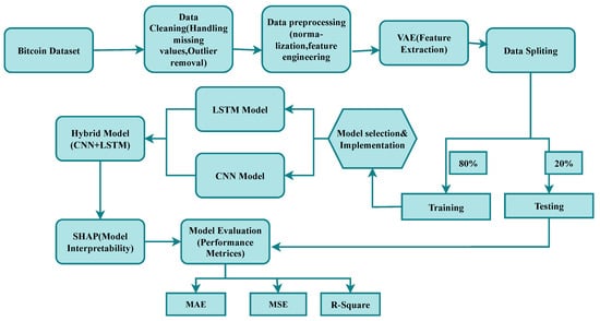
Figure 1.
Bitcoin price prediction pipeline using VAE, also implementing an interpretability-enhancing hybrid CNN-LSTM model with SHAP.
3.1. Data Collection
The dataset used for the current research comprises historical Bitcoin prices including elements such as open, high, low, close, and volume, as demonstrated in Table 2. The information can be collected through freely accessible websites such as Kaggle [21]. The dataset encompasses a particular time frame of the years 2013–2021 to give adequate historical information for training and testing. Every data point contains a particular date, which is needed for time-series analysis. Moreover, the dataset originally contains columns such as ‘Name’, ‘Symbol’, and ‘Marketcap’, which are irrelevant for price prediction and are deleted during preliminary processing.
Table 2.
Bitcoin price prediction (2013–2021) historical data.
3.2. Data Preprocessing
A variety of planning techniques are employed to guarantee the reliability of the data. The initial analysis shows that the dataset does not contain missing values. To keep the time-series framework, the ‘Date’ column is changed into a DateTime format and allocated as an index. Duplicate records are also eliminated to avoid redundancy. Non-essential columns such as ‘Name’, ‘Symbol’, and ‘Marketcap’ are dropped to focus only on numerical attributes. The numerical features (‘High’, ‘Low’, ‘Open’, ‘Close’, and ‘Volume’) are then normalized using Min-Max Scaling (Equation (2)), which transforms the values into a range between 0 and 1. This normalization helps improve model performance by ensuring all features contribute equally to predictions.
normalizes the feature values to a range of [0, 1].
- a: The original data value (e.g., Bitcoin price features like High, Low, Open, Close, Volume).
- : The minimum value in the dataset for a specific feature.
- : The maximum value in the dataset for the same feature.
- : The transformed value after normalization.
This scaling ensures that all features have the same range, improving the performance of deep-learning models like CNN, LSTM, and CNN-LSTM in your Bitcoin price prediction task.
Finally, the cleaned and scaled dataset is split into training (80%) and testing (20%) sets, keeping sequential to maintain the time-series nature of Bitcoin price data. Each sequence is of a fixed time step number (e.g., 30 days) and is used as input to the model as shown in Table 3.
Table 3.
Data preprocessing includes outlier removal and normalization.
3.3. Augmented Dickey-Fuller (ADF) Testing
We applied the ADF test to evaluate the stationarity of the input time series for features Open, High, Low, Close, and Volume. This statistical testing ensures alignment with traditional econometric practices and increases the interpretability of our preprocessing pipeline. The ADF statistic test results in Table 4 show that all input features are non-stationary, with p-values exceeding 0.05 and test statistics not less than the critical values at the 5% significance level. Therefore, the null hypothesis of a unit root could not be rejected.
Table 4.
ADF test results for stationarity: statistical test.
3.4. Feature Extraction: VAE
Specific characteristics are obtained from the preprocessed information using the VAE. An encoder, a space with latent information, and a decoder are characteristics of the VAE model. The information that is input is expressed in latent space by the encoder. ReLU functions for activation and numerous dense layers offer the model the potential to acquire knowledge. The information’s irregular connections. The encoder shrinks the original input data before translating it into a lower-dimensional space known as latent. Furthermore, to be expressed as a distribution of probabilities, the latent space maintains the shortened form of the input data. This enables VAE to figure out the fundamental structure of data and synthesize new information samples. Conversely, the decoder translates the latent space structure of the provided data backwards to the actual input data. Furthermore, it contains dense layers that reconstruct the actual data from the shortened form using ReLU activation functions. The VAE is trained using a loss function that includes KL divergence (to regulate the latent space) and reconstruction loss (to properly rebuild the given input data). By acquiring a compact latent representation of the input data, the VAE increases the hybrid CNN-LSTM model’s capacity to extract intricate patterns from Bitcoin prices.
For feature extraction from Bitcoin price data. First, the cleaned and scaled dataset is reloaded, and the data are split into training and testing sets without shuffling to preserve the time-series order. The VAE consists of an encoder and a decoder. The encoder takes the input features and processes them through a dense layer with ReLU activation. It creates two outputs for the latent space depiction: the mean (z_mean) and the logarithm of variance (z_log_var). A random sampling function produces latent variables using a reparameterization technique, letting the model to acquire continual valuable data Latent space. The decoder rebuilds input data from the latent space using dense layers and produces a feature representation with sigmoid activation. The VAE model is generated with the Adam optimizer and mean squared error (MSE) loss function. To guarantee TensorFlow connectivity, the dataset is initially converted to float32. The model is trained over 50 epochs with a batch size of 32, employing training data as input and target, and verified on the test set. Finally, the trained VAE is used to produce latent feature representations (X_train_vae and X_test_vae), which can serve as input features in later Bitcoin price prediction models.
The latent space dimension of the VAE was empirically selected. Various latent sizes were tested, and a dimension of 16 was finalized as it offered a suitable trade-off between compression and reconstruction accuracy. This latent space effectively captured informative features for downstream CNN-LSTM prediction.
3.5. Applied Neural Networks
3.5.1. Convolutional Neural Network (CNN)
We used a CNN [22] for Bitcoin price prediction using historical price data. The dataset is first loaded and split into features (X) and the target variable (y), where the ‘Close’ price is used as the prediction target. Since CNNs require input in a specific format, X is reshaped into a 3D array with dimensions (samples, time steps, features). The data are then divided into training and testing sets without shuffling to maintain the sequential nature of time-series data.
The CNN model is built using the Sequential API in Keras. It starts with a Conv1D layer with 64 filters and a kernel size of 3, which extracts important patterns from the sequential data by applying convolutional operations. This layer helps identify local trends in Bitcoin price movement. Next, a MaxPooling1D layer with a pool size of 2 is used to reduce the dimensionality of the feature maps, retaining essential information while preventing overfitting. Following the feature extraction process, a Flatten() layer flattens the multi-dimensional result into a 1D vector that might be forwarded to fully connected layers. To collect complicated connections between features, a dense layer containing 64 neurons and ReLU activation occurs next. One unactivated neuron, which is suitable for regression tasks, serves up the last output layer, which estimates the closing price of Bitcoin.
For regression problems, the Adam optimizer and mean squared error (MSE) loss function are used for constructing the model. With a batch size of 32, the model is trained over 50 epochs, implementing training data for learning and validation data for measuring performance. Afterwards training, predictions are calculated on the test set, and the model’s fit to the data is determined using the mean squared error (MSE), mean absolute error (MAE), and R2 value. The plotting of the loss over time and combining real and forecasted Bitcoin prices facilitates a visual representation of the consequences. In the end, Google Drive can be utilized for storing the trained model for use afterwards.
3.5.2. Long Short-Term Memory (LSTM) Network
We used an LSTM neural network [23] for Bitcoin price prediction using historical data. The dataset is first loaded, and the relevant numerical features (‘High’, ‘Low’, ‘Open’, ‘Close’, and ‘Volume’) are extracted as input (X), while the ‘Close’ price is chosen as the target variable (y). Since LSTMs require sequential input, X is reshaped into a 3D format with dimensions (samples, time steps, features). The data are then split into training and testing sets without shuffling to maintain the time-series order.
The LSTM model is constructed using the Sequential API in Keras. It begins with an LSTM layer containing 64 units and ReLU activation, which helps capture long-term dependencies in the sequential Bitcoin price data. To generate estimations, the LSTM layer investigates historical price fluctuations to determine shifts. The gathered structures are ultimately improved via the addition of a Dense layer with 64 neurons and ReLU activation. One unactivated neuron comprises the last output layer, which is used for regression tasks, including forecasting the coming closing price of Bitcoin. The mean squared error (MSE) loss function and Adam optimizer, which perform well for problems related to regression, are employed to generate the model.
Following this, the model is trained for 50 epochs with a batch size of 32, and its performance can be monitored using validation data. Throughout training, predictions are made for the test set, and the model’s performance can be assessed via performance metrics, which include mean squared error (MSE), mean absolute error (MAE), and R2 value. Two plots have been generated to demonstrate what was found: one contrasts the actual and predicted Bitcoin prices, while another illustrates the loss over epochs for both the training and validation sets. At last, Google Drive can be utilized for storing the trained LSTM model for use afterwards. This technique makes use of LSTM’s potential for identifying linear relationships, which enables it to evaluate the price of Bitcoin.
3.5.3. Proposed Hybrid CNN-LSTM Model
The supplied code integrates the incremental learning abilities of long short-term memory (LSTM) networks with the feature extraction skills of convolutional neural networks (CNNs) to generate a hybrid CNN-LSTM model for Bitcoin price prediction. When the dataset is newly loaded, it shows the appropriate numerical parameters (‘High’, ‘Low’, ‘Open’, ‘Close’, and ‘Volume’ are chosen as inputs (X), and the goal variable (y) is the ‘Close’ price. The feature matrix is reshaped to correspond to the 3D input style that LSTMs demand. For the sake of the consistency of the time series, the data are separated into training and testing sets without being randomized.
The hybrid CNN-LSTM model is developed with 64 filters and a kernel size of 3. The first layer is a 1D convolutional layer that captures meaningful spatial patterns from alterations in the price of Bitcoin. By maintaining the most essential characteristics, the MaxPooling layer decreases dimensionality and promotes computational speed. An LSTM layer with 64 units is added after the feature extraction procedure to detect temporal dependencies and facilitate the model’s interpretation of long-term trends in Bitcoin prices. A Dense layer with 64 neurons collects the output from the LSTM layer to further develop the designs that have been gained. In the end, regression is conducted with a single neuron output layer to predict the closing price of Bitcoin. The mean squared error (MSE) loss function and Adam optimizer, both of which are suitable for time-series prediction, are implemented for constructing the model. A batch size of 32 is utilized for training throughout 50 epochs, and results are observed using validation data. Immediately after training, predictions are produced on the test set, and the reliability of the predictions is determined via evaluation metrics that involve mean squared error (MSE), mean absolute error (MAE), and R2 value.
Two graphs are produced to demonstrate the model’s effectiveness: one combines real and forecast Bitcoin prices, and the additional one illustrates the loss pattern throughout epochs for both training and validation sets. The trained CNN-LSTM model is subsequently saved as a file for later usage, providing real-time implementation or further validation. This hybrid technique efficiently forecasts the price of Bitcoin by using CNN’s ability to determine specific trends and LSTM’s capability to control time-series connections.
Modular computational complexity analysis:
Let:
- T = Number of time steps (sequence length)
- F = Number of input features
- K = Convolution kernel size
- H = Number of LSTM hidden units
- D = Latent dimension in the VAE
The approximate time complexity of each component is:
Thus, the overall complexity of the proposed hybrid model is primarily linear to quadratic in the input size and hidden layer dimensions during training and inference, with SHAP incurring additional post-hoc computational cost only during interpretability analysis, not affecting model deployment efficiency. Each model architecture is expressed in Table 5.
Table 5.
Parameter count and main strengths of compared models.
Regularization strategies:
To prevent overfitting and ensure robust generalization, multiple regularization techniques are integrated into the model architecture:
- Dropout layers with a rate of 0.2 were inserted after both convolutional and LSTM layers to deactivate neurons during training and reduce co-adaptation randomly.
- L2 weight regularization (1 × 10 −4) was applied to Conv1D, LSTM, and Dense layers, penalizing large weights to control model complexity.
- EarlyStopping was employed to halt training when validation loss ceased to improve, thereby avoiding overfitting.
These strategies are implemented in the updated architecture and significantly contributed to the model’s generalization on unseen test data.
3.6. SHAP for Interpretability
The objective of this program is to import a trained Hybrid CNN-LSTM model and understand its forecasts via SHAP [24]. Determining the way that each of the given features—“High”, “Low”, “Open”, “Close”, and “Volume”—contributes to the expected closing price of Bitcoin is the primary objective of implementing SHAP. Through the use of SHAP, we can understand how multiple factors affected the model’s choice-making, which shows the deep-learning method’s clearness. The initial phase is to utilize TensorFlow’s load_model() method to import the already trained Hybrid CNN-LSTM model from a stored file. This model was trained on historical Bitcoin price data, where it learned patterns using convolutional layers (CNN) for feature extraction and LSTM layers for capturing temporal dependencies. Once the model is loaded, we prepare the test data (X_test). If actual test data are unavailable, the code generates a synthetic dataset containing random values. Since the CNN-LSTM model expects data in a 3D format (samples, time steps, features), the test data are reshaped accordingly.
To make SHAP work with the CNN-LSTM model, a wrapper function (model_wrapper()) is created. This function reshapes SHAP’s 2D input into the required 3D format before making predictions. SHAP’s KernelExplainer is then initialized using a subset of the test data (first 100 samples) as a background dataset. The KernelExplainer method is computationally expensive, so using a smaller dataset helps improve efficiency while still providing meaningful insights.
The SHAP clarification determines SHAP values, indicating every feature’s impact on the model’s forecasting, after it has been adjusted. In a bid to make the SHAP values clearer to comprehend if the shape of the result is 3D, the figures are averaged throughout the third dimension to make them 2D. Two essential plots—the force graph and the summary graph—are then used to demonstrate the estimated SHAP values. The summary plot highlights which features have the most significant effect on Bitcoin price forecasts by illustrating the total effect of every variable throughout all test samples. A more comprehensive review of a single forecast can be obtained by the force plot, which demonstrates how every element influences the expected closing price.
Implementing SHAP onto the Hybrid CNN-LSTM model offers the primary benefit of boosting model openness, letting us gain insight into the various ways in which specific factors affect fluctuations in the price of Bitcoin. In financial applications, where recognizing the reason for supporting model forecasts can promote confidence and boost choices, this clarity becomes especially important. Deep learning and readability approaches like SHAP are utilized in this method to make sure that the model’s conclusions are not only right but also understood and reasonable.
3.7. Hyperparameter Selection
The hyperparameters used in our CNN-LSTM model, including the number of filters, kernel size, LSTM units, dropout rates, batch size, and regularization parameters, were selected based on preliminary experiments and established practices from relevant literature. These choices aimed to balance model accuracy and training stability while preventing overfitting, as shown in Table 6. To select hyperparameters, we performed a random search approach. The early stopping mechanism is employed to avoid overfitting and ensure good generalization.
Table 6.
Selected hyperparameters review.
3.8. Performance Evaluation
Three essential metrics [25] mean squared error (MSE), mean absolute error (MAE), and R-squared (R2) are applied in evaluating the efficiency of the proposed approach. The MSE provides an indicator of the reliability of the model by standardizing the squared difference between real and predicted values. An indicator of the model’s sensitivity to anomalies, the MAE indicates the average absolute difference between actual and expected values. The quality of performance is demonstrated by the R2, which reflects how much variance is determined by the model. To identify the superior performance, the proposed method can be compared with basic models, specifically CNN alone, LSTM alone, and hybrid CNN-LSTM with VAE.
The outcome of the models is evaluated using the metrics calculations shown below:
3.8.1. Mean Absolute Error (MAE)
The mean absolute error (MAE) is a prominent regression analysis statistic that determines the average difference between real and anticipated values. Mathematically, it is represented as (Equation (2)):
In the above formula, n shows the total number of observations, indicates the current Bitcoin price, and indicates the expected value. The absolute difference ensures that both overestimation and underestimation contribute equally to the error. The sum aggregates these errors across all measurements, and dividing by n yields the average deviation. MAE is expressed in the same units as the target variable, enabling a straightforward understanding of prediction error. A lower MAE indicates higher prediction accuracy, signifying that the model’s forecasts are closer to real values.
3.8.2. Mean Squared Error (MSE)
The mean squared error (MSE) is a commonly used statistic in regression analysis that predicts the average squared difference between parameters. Mathematically, it is defined as (Equation (3)):
In the above equation, n refers to the total number of observations, is the actual Bitcoin price at the time, and is the anticipated value. Each data point’s error is squared to account for both positive and negative contributions to the aggregate error. The squared errors are summed across all observations and averaged by dividing by n to calculate the final MSE value. Due to squaring, larger differences have a greater impact on the final score, making MSE highly sensitive to anomalies. A lower MSE denotes a more accurate model, reflecting smaller discrepancies between predicted and actual values.
3.8.3. R-Squared ()
The coefficient of determination () measures the proportion of variance in Bitcoin prices explained by the model. A higher score (close to 1) suggests better forecasting precision. It is mathematically expressed as (Equation (4)):
Here, is the actual Bitcoin price, is the expected value, and is the mean of all actual values. The numerator represents the mean squared error (MSE), while the denominator indicates the variance in the actual prices. The value ranges from 0 to 1. A model with an close to 1 reliably forecasts Bitcoin values, whereas a lower suggests poor model performance in capturing price variations. This metric is crucial for evaluating a model’s fit and its accuracy in predicting Bitcoin price trends.
4. Results and Discussions
The hybrid CNN-LSTM model, supplemented with VAE and SHAP, is assessed using three crucial metrics: MSE, MAE, and R2. The results are compared with baseline models, including standalone CNN, standalone LSTM, and hybrid CNN-LSTM with VAE.
4.1. Results with Standalone CNN Model
The CNN model achieves an MSE of 0.0005, an MAE of 0.012, and an R2 score of 0.99. While CNNs are very gifted at recognizing spatial patterns and building hierarchies of features as shown in Figure 2b, they are not good at recognizing the sequential dependencies typical of time-series data, such as in Table 7. Since the volatility of cryptocurrency prices is influenced by past trends, the isolated CNN model cannot recognize the temporal relationships involved. Therefore, while CNN can learn meaningful representations from the dataset, its failure to recognize long-term dependencies leads to high errors compared to both the LSTM and CNN-LSTM hybrid models. It converges quickly but may overfit due to its focus on spatial features. Validation loss might be higher compared to other models, as in Figure 2a.
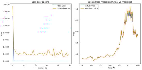
Figure 2.
Comparison of the true price of Bitcoin and predicted price based on (CNN Model) that extracts spatial features from historical price data to identify patterns and trends. Here (a) indicates the validation and train loss, converges quickly but may overfit due to its focus on spatial features and (b) indicates the actual vs. predicted price.
Table 7.
CNN model evaluation performance metrics scores.
4.2. Results with Standalone LSTM Model
The LSTM model remedies CNN’s weakness by learning temporal connections in the data efficiently. The LSTM model has a lower MSE of 0.0007, MAE of 0.019, and greater R2 of 0.98, compared to the standalone CNN model as shown in Table 8. However, despite improved performance, the LSTM model is still short of completely optimizing feature extraction as in Figure 3b. While it learns temporal relationships efficiently, the LSTM model lacks the strong spatial feature extraction benefit of CNN, which is so efficient in detecting local trends of price movements. This weakness renders the LSTM model unable to achieve the minimum possible error as shown in Figure 3a. It learns temporal dependencies well but converges more slowly. It may generalize better, reducing validation loss.
Table 8.
LSTM model evaluation performance metrics scores.
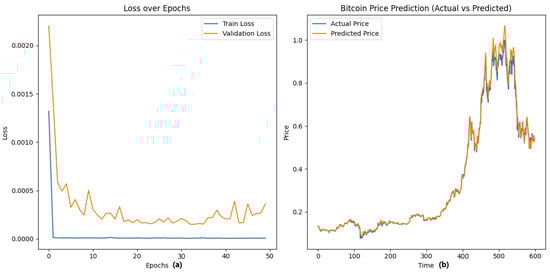
Figure 3.
Comparison of the true price of Bitcoin and predicted price based on (LSTM model) that captures temporal dependencies in historical price data to improve forecasting accuracy. Here (a) indicates the validation and train loss, which may generalize better, reducing validation loss, and (b) indicates the actual vs. predicted price.
4.3. Results with Hybrid CNN-LSTM Model
The hybrid CNN-LSTM model, enhanced by VAE, performs the best among all the models experimented with. The model achieves an MSE of 0.0002, MAE of 0.008, and an R2 score of 0.99, demonstrating its better capacity for capturing spatial and temporal correlations in Bitcoin price dynamics. With CNN for feature extraction and LSTM for sequential modeling combined, the hybrid model leverages the best from both architectures. The inclusion of VAE enhances the feature space further, learning latent representations to enable the model to recognize hidden patterns in Bitcoin price data. This largely minimizes noise and redundancy in the dataset, delivering more accurate and stable predictions. Moreover, with the addition of VAE-based feature extraction, the MAE further reduces to 0.0001, with an R2 score of 0.98 as evidenced in Table 9. This indicates that VAE improves the quality of features extracted, enabling the model to concentrate on the most relevant features of price behaviour. Figure 4b illustrates how the hybrid CNN-LSTM model with VAE delivers the best predictions, most closely reflecting actual Bitcoin price fluctuations as evident. On the other hand, combines spatial and temporal learning, leading to better generalization and likely the lowest validation loss as shown in Figure 4a.
Table 9.
Hybrid CNN-LSTM model evaluation performance metrics scores.
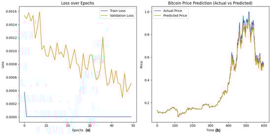
Figure 4.
Comparison of the true price of Bitcoin and predicted price based on (Hybrid CNN-LSTM model) that combines CNN’s with LSTM’s ability to capture temporal dependencies, enhancing predictive accuracy. Here (a) indicates the validation and train loss and combines spatial and temporal learning, leading to better generalization and likely the lowest validation loss, and (b) indicates the actual vs. predicted price.
4.4. Walk-Forward Validation: 5-Folds
We implemented a walk-forward validation strategy to address concerns regarding the reliability and generalizability of the evaluation metrics. The dataset is split into five sequential folds, and the proposed model is trained on all prior data and tested on the subsequent fold, preserving the temporal dependencies of the financial time series. We computed the MSE, MAE, and R2 score for each fold and reported these metrics’ mean and standard deviation across all five folds. These values reflect the consistency and robustness of the proposed model, as shown in Table 10.
Table 10.
Performance metrics with walk-forward validation (Mean ± Std).
4.5. SHAP Analysis for Improved Interpretability
To ensure transparency and explanations are provided about the predictions made by the model, SHAP is employed in an attempt to investigate the contribution of different features towards predicting the price of Bitcoin. While the use of SHAP does not affect the model performance metrics directly, it provides necessary explanations about feature contributions towards predictions made by the model, as seen in Table 11.
Table 11.
SHAP model explainability feature values.
- Open price (SHAP value: 0.45) is the most important variable in model predictions, indicating that the opening price of the market is important in predicting future price movement.
- High price (SHAP value: 0.35) is the second most influential attribute, i.e., the highest price seen during a trading period significantly affects the accuracy of forecasts.
- Low price (SHAP value: 0.12), while it is a significant attribute, is less significant to the model’s behavior than open and high prices.
- Closing price (SHAP value: 0.06) shows a low impact on predictions, indicating that its predictive ability is lower than expected.
- Trading volume (SHAP value: 0.02) is the least important feature, and indicates that trading volume has no or negligible impact on Bitcoin price prediction in this model.
By utilizing SHAP analysis, the model gains interpretability, allowing researchers and traders to understand which factors drive Bitcoin price changes the most. This enhances trust in the model and provides useful insights for financial decision making as shown in Figure 5.
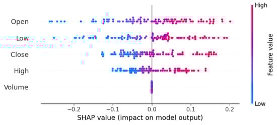
Figure 5.
SHAP for model interpretability: Identifies the most influential features affecting Bitcoin price predictions, enhancing transparency and explainability.
4.6. Ablation Study Analysis
We have performed an ablation comparison in Table 12, showing the standalone CNN, standalone LSTM, hybrid CNN-LSTM (without VAE and SHAP), and hybrid CNN-LSTM with VAE. The results clearly show performance improvement when VAE is added. While SHAP does not alter prediction accuracy, it significantly enhances model interpretability. This ablation study’s final model (CNN-LSTM + VAE + SHAP) balances performance and transparency best.
Table 12.
Ablation study showing performance with and without VAE and SHAP.
4.7. Comparison with State-of-the-Art Studies
The comparative performance analysis of our novel proposed Bitcoin price prediction with other state-of-the-art studies is examined in Table 13. For a fair comparison, we reported performance metrics from different studies on a similar dataset and compared them with the results of our proposed model. Early methods, such as ARIMA and SVMs, struggled to capture the highly volatile and non-linear nature of cryptocurrency prices. With the rise of deep learning, hybrid models like CNN-LSTM have gained prominence due to their ability to capture both spatial and temporal dependencies. Recent research efforts have boosted predictability through the use of mechanisms related to attention, ensemble techniques, and explainability tools like SHAP. The TFT is a leading model for multi-horizon forecasting, with excellent accuracy through attention-based mechanisms. However, many existing approaches lack feature refinement, interpretability, and computational efficiency. This innovative method improves the features.
Table 13.
The comparative performance analysis of the proposed approach with the other state-of-the-art studies.
Though widely used, traditional models such as ARIMA and GARCH often fail to capture Bitcoin prices’ non-linear and temporal dynamics. We included ARIMA and GARCH in our experiments to serve as baseline comparisons. The ARIMA model is applied for univariate price prediction, while the GARCH model is used for volatility forecasting. The performance of each model is evaluated using MSE, MAE, and R2 score, as shown in Table 14.
Table 14.
Comparison of deep-learning model with statistical baselines (ARIMA, GARCH).
4.8. Residual Diagnostics: ACF and PACF Test
We conducted a thorough residual analysis to validate the assumptions underlying our time-series model. Specifically, we examined the autocorrelation structure and potential heteroskedasticity of the residuals produced by our proposed hybrid CNN-LSTM model. We computed the residuals’ autocorrelation function (ACF) and partial autocorrelation function (PACF) to assess serial dependence. The plots are shown in Figure 6. Visual inspection reveals that the autocorrelations of the residuals fall within the 95% confidence intervals, indicating the residuals approximate white noise behavior. This suggests that the model has successfully captured the temporal dependencies in the data, and no significant autocorrelation remains.
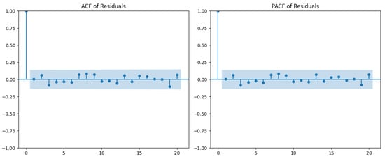
Figure 6.
ACF and PACF of residuals from the CNN-LSTM model.
4.9. Comparison of Proposed Architecture over Transformer Models
While hybrid models integrating CNN, LSTM, VAE, and SHAP have appeared in financial forecasting literature, our contribution lies in the structured stream that combines these techniques to enhance interpretability and robust feature learning. SHAP adds transparency to the whole pipeline. To highlight the theoretical motivation behind our model choice over SHAP-based Transformer models, we provide a comparative overview in Table 15.
Table 15.
Comparative theoretical overview of proposed model vs. transformer-based SHAP models.
4.10. Practical Application
Although the current study focuses on developing and validating a hybrid CNN-LSTM + VAE deep-learning model for cryptocurrency price prediction, we envision several practical applications that highlight the broader impact of our work. The potential applications include:
- Risk analysis: Utilizing the model’s predictive outputs to assess market risk and inform hedging strategies.
- Portfolio optimization: Integrating predictions into portfolio allocation algorithms to optimize returns under risk constraints.
- Algorithmic trading: Embedding the model within automated trading systems for generating buy/sell signals based on predicted price movements.
Future work will focus on implementing backtesting environments and live trading simulations to rigorously evaluate the model’s performance in operational settings. Additionally, incorporating transaction costs, slippage, and order execution dynamics will be essential for real-world deployment. This application perspective underscores the practical relevance of our model and motivates further research to bridge the gap between deep-learning research and financial market operations.
4.11. Study Limitations
SHAP requires evaluating changes in model output through feature perturbations, which becomes computationally expensive for deep architectures with high-dimensional input spaces. Another limitation arises from SHAP’s assumption of feature independence during perturbation. In time-series models like CNN-LSTM, temporal features are inherently correlated and contextually dependent. This independence assumption is thus not strictly valid, which may affect the fidelity of the explanations.
5. Conclusions and Future Work
Estimating Bitcoin prices can be tricky due to market swings and irregularity. This paper introduces a hybrid deep-learning model with feature-extraction techniques, which includes a CNN, to successfully address the challenge. Combining CNN and LSTM systems, we believe that boost Bitcoin price anticipating accuracy significantly. Moreover, VAE has been applied to extract features and enhance data representation. Additionally, SHAP has been used to endow the model with interpretability by carefully examining the contribution of different features used in the forecasting process.
The experimental findings of the current study established that the CNN-LSTM model, which has been successfully combined with the VAE, performed at a level regarded as being superior, with an MSE of 0.0002, an MAE of 0.008, and a remarkable R-squared (R2) of 0.99. These precise values conclusively imply that the suggested hybrid model not only performs efficiently but also effectively captures the intricate dynamics involved with the price movements of Bitcoin, thus outperforming conventional machine-learning techniques as well as other deep-learning techniques employed for comparison.
By minimizing noise and strengthening the model’s expansion, the use of VAE significantly boosted feature extraction. Furthermore, the SHAP system boosted clearness by enabling users to find out how different characteristics impact estimations. Investors and financial analysts should be conscious of this since they demand efficient and intelligible prediction models. At last, this detailed examination demonstrates how effectively hybrid deep-learning models performed in the difficult task of financial time-series forecasting. Additionally, future studies can look into integrating attention mechanisms, reinforcement-learning techniques, or even other market predictors to enhance the accuracy and uniformity of this prediction.
The recommended hybrid CNN-LSTM model for Bitcoin price estimation could be refined in several ways in future investigations. One interesting establishment is the invention of a real-time prediction system that combines high-frequency data sources with outside influences like social media sentiment and macroeconomic indices. Advanced hyperparameter optimization procedures and ensemble strategies could be utilized to enhance forecast accuracy. By extending the model for various other cryptocurrencies and other sectors like stock market forecasting, its ability to be generalized could be increased. Advanced explainability methodologies like LIME and Grad-CAM could be used with SHAP to deliver deeper interpretability, and reinforcement learning might be employed in constructing flexible trading strategies. Furthermore, we plan to enhance the model by incorporating external features such as macroeconomic indicators, social media sentiment, and blockchain-level (on-chain) metrics. These inputs may further improve robustness and generalization.
Author Contributions
Conceptualization, W.B., S.R., A.R., N.L.F., M.S. and S.W.L.; Methodology, W.B., N.L.F., M.S. and S.W.L.; Software, W.B.; Validation, S.R. and A.R.; Formal analysis, W.B., N.L.F. and M.S.; Investigation, S.R. and A.R.; Data curation, W.B., S.R. and A.R.; Writing—original draft, W.B., S.R., A.R. and N.L.F.; Writing—review & editing, N.L.F., M.S. and S.W.L.; Visualization, W.B., N.L.F. and M.S.; Supervision, S.R., M.S. and S.W.L.; Funding acquisition, M.S. and S.W.L. All authors have read and agreed to the published version of the manuscript.
Funding
This research was supported by the SungKyunKwan University and the BK21 FOUR (Graduate School Innovation) funded by the Ministry of Education (MOE, Korea) and National Research Foundation of Korea (NRF). This work was also supported by National Research Foundation (NRF) grants funded by the Ministry of Science and ICT (MSIT) and Ministry of Education (MOE), Republic of Korea (NRF[2021-R1-I1A2(059735)]; RS[2024-0040(5650)]; RS[2024-0044(0881)]; RS[2019-II19(0421)]).
Data Availability Statement
This research was conducted using the publicly available Cryptocurrency Historical Prices dataset, which can be accessed at https://www.kaggle.com/datasets/sudalairajkumar/cryptocurrencypricehistory/data (accessed on 9 April 2025).
Conflicts of Interest
The authors declare no conflicts of interest.
References
- Kazeminia, S.; Sajedi, H.; Arjmand, M. Real-Time Bitcoin Price Prediction Using Hybrid 2D-CNN LSTM Model. In Proceedings of the 2023 9th International Conference on Web Research (ICWR), Tehran, Iran, 3–4 May 2023; pp. 173–178. [Google Scholar] [CrossRef]
- Peng, P.; Chen, Y.; Lin, W.; Wang, J.Z. Attention-based CNN–LSTM for high-frequency multiple cryptocurrency trend prediction. Expert Syst. Appl. 2024, 237, 121520. [Google Scholar] [CrossRef]
- Chen, S.; Liao, Z.; Zhang, J. Forecasting the Price of Bitcoin Using an Explainable CNN-LSTM Model. In Intelligent Computers, Algorithms, and Applications; Cruz, C., Zhang, Y., Gao, W., Eds.; Springer: Singapore, 2024; Volume 2036, pp. 1–15. [Google Scholar] [CrossRef]
- Mehra, M.K.; Tyagi, S.; Kanthalia, T.; Shree, R.K.; Chaturvedi, P.; Singh, P. Evaluating LSTM and GRU Models for Cryptocurrency Price Forecasting in Financial Markets. In Proceedings of the 2023 3rd International Conference on Technological Advancements in Computational Sciences (ICTACS), Tashkent, Uzbekistan, 1–3 November 2023; pp. 425–431. [Google Scholar] [CrossRef]
- Pujitha, M.V.; Kumar, K.S.; Sree, D.I.; Devi, P.Y. Predicting Bitcoin Prices for the Next 30 Days Using LSTM-Based Time Series Analysis. In Proceedings of the 2023 2nd International Conference on Futuristic Technologies (INCOFT), Belagavi, Karnataka, India, 24–26 November 2023; pp. 1–8. [Google Scholar] [CrossRef]
- Singathala, H.; Malla, J.; Jayashree, J.; Vijayashree, J. A Deep Learning based Model for Predicting the future prices of Bitcoin. In Proceedings of the 2023 2nd International Conference on Vision Towards Emerging Trends in Communication and Networking Technologies (ViTECoN), Vellore, India, 5–6 May 2023; pp. 1–4. [Google Scholar] [CrossRef]
- Mansourabady, F.; Tabe, A.H.; Rasekh, A.; Ghermezian, A. A Study on Hybrid Deep Learning Approaches for “Monero” Cryptocurrency Price Prediction. In Proceedings of the 2024 20th CSI International Symposium on Artificial Intelligence and Signal Processing (AISP), Babol, Iran, 21–22 February 2024; pp. 1–6. [Google Scholar] [CrossRef]
- Oyedele, A.A.; Ajayi, A.O.; Oyedele, L.O.; Bello, S.A.; Jimoh, K.O. Performance evaluation of deep learning and boosted trees for cryptocurrency closing price prediction. Expert Syst. Appl. 2023, 213, 119233. [Google Scholar] [CrossRef]
- Rathee, N.; Singh, A.; Sharda, T.; Goel, N.; Aggarwal, M.; Dudeja, S. Analysis and price prediction of cryptocurrencies for historical and live data using ensemble-based neural networks. Knowl. Inf. Syst. 2023, 65, 4055–4084. [Google Scholar] [CrossRef]
- Peng, Y.; Yang, X.; Li, D.; Ma, Z.; Liu, Z.; Bai, X.; Mao, Z. Predicting flow status of a flexible rectifier using cognitive computing. Expert Syst. Appl. 2025, 264, 125878. [Google Scholar] [CrossRef]
- Peng, Y.; Sakai, Y.; Funabora, Y.; Yokoe, K.; Aoyama, T.; Doki, S. Funabot-Sleeve: A Wearable Device Employing McKibben Artificial Muscles for Haptic Sensation in the Forearm. IEEE Robot. Autom. Lett. 2025. [Google Scholar] [CrossRef]
- Kim, T.Y.; Cho, S.B. Predicting the direction of stock price index movement using LSTM with technical indicators. Expert Syst. Appl. 2019, 116, 279–290. [Google Scholar]
- Chen, Y.; Lin, W.; Wang, J.Z. A hybrid CNN-LSTM model for stock market prediction. J. Comput. Sci. 2021, 52, 101239. [Google Scholar]
- Makridakis, S.; Spiliotis, E.; Assimakopoulos, V. Statistical and Machine Learning forecasting methods: Concerns and ways forward. PLoS ONE 2018, 13, e0194889. [Google Scholar] [CrossRef] [PubMed]
- Hyndman, R.J.; Athanasopoulos, G. Forecasting: Principles and Practice; OTexts: Melbourne, Australia, 2018. [Google Scholar]
- Taylor, S.J.; Letham, B. Forecasting at scale. Am. Stat. 2018, 72, 37–45. [Google Scholar] [CrossRef]
- Smyl, S. A hybrid method of exponential smoothing and recurrent neural networks for time series forecasting. Int. J. Forecast. 2020, 36, 75–85. [Google Scholar] [CrossRef]
- Goodfellow, I.; Bengio, Y.; Courville, A. Deep Learning; MIT Press: Cambridge, MA, USA, 2016. [Google Scholar]
- Lundberg, S.M.; Lee, S.I. A unified approach to interpreting model predictions. In Advances in Neural Information Processing Systems; NIPS Foundation: La Jolla, CA, USA, 2017; Volume 30. [Google Scholar]
- Lim, B.; Arık, S.O.; Loeff, N.; Pfister, T. Temporal Fusion Transformers for interpretable multi-horizon time series forecasting. Int. J. Forecast. 2021, 37, 1748–1764. [Google Scholar] [CrossRef]
- SRK. Cryptocurrency Historical Prices. Available online: https://www.kaggle.com/datasets/sudalairajkumar/cryptocurrencypricehistory (accessed on 9 April 2025).
- Raza, A.; Younas, F.; Siddiqui, H.U.R.; Rustam, F.; Villar, M.G.; Alvarado, E.S.; Ashraf, I. An improved deep convolutional neural network-based YouTube video classification using textual features. Heliyon 2024, 10, e35812. [Google Scholar] [CrossRef] [PubMed]
- Alam, A.; Raza, A.; Thalji, N.; Abualigah, L.; Garay, H.; Iturriaga, J.A.; Ashraf, I. Novel transfer learning approach for hand drawn mathematical geometric shapes classification. Peerj Comput. Sci. 2025, 11, e2652. [Google Scholar] [CrossRef] [PubMed]
- Raza, A.; Eid, F.; Montero, E.C.; Noya, I.D.; Ashraf, I. Enhanced interpretable thyroid disease diagnosis by leveraging synthetic oversampling and machine learning models. BMC Med. Inform. Decis. Mak. 2024, 24, 364. [Google Scholar] [CrossRef] [PubMed]
- Raza, A.; Rustam, F.; Siddiqui, H.U.R.; Flores, E.S.; Mazón, J.L.V.; de la Torre Díez, I.; Ripoll, M.A.V.; Ashraf, I. Ventilator pressure prediction employing voting regressor with time series data of patient breaths. Health Inform. J. 2025, 31, 14604582241295912. [Google Scholar] [CrossRef] [PubMed]
- Zhang, X.; Zhang, Y. A deep learning approach for Bitcoin price prediction using LSTM. J. Comput. Sci. 2020, 45, 101181. [Google Scholar]
- Fawaz, H.I.; Forestier, G.; Weber, J.; Idoumghar, L.; Muller, P.A. Deep learning for time series classification: A review. Data Min. Knowl. Discov. 2019, 33, 917–963. [Google Scholar] [CrossRef]
- Borovykh, A.; Bohte, S.; Oosterlee, C.W. Conditional time series forecasting with convolutional neural networks. arXiv 2017, arXiv:1703.04691. [Google Scholar]
- Qin, Y.; Song, D.; Chen, H.; Cheng, W.; Jiang, G.; Cottrell, G.W. A dual-stage attention-based recurrent neural network for time series prediction. arXiv 2017, arXiv:1704.02971. [Google Scholar]
Disclaimer/Publisher’s Note: The statements, opinions and data contained in all publications are solely those of the individual author(s) and contributor(s) and not of MDPI and/or the editor(s). MDPI and/or the editor(s) disclaim responsibility for any injury to people or property resulting from any ideas, methods, instructions or products referred to in the content. |
© 2025 by the authors. Licensee MDPI, Basel, Switzerland. This article is an open access article distributed under the terms and conditions of the Creative Commons Attribution (CC BY) license (https://creativecommons.org/licenses/by/4.0/).