L^p-Norm for Compositional Data: Exploring the CoDa L¹-Norm in Penalised Regression

Abstract

The Least Absolute Shrinkage and Selection Operator (LASSO) regression technique has proven to be a valuable tool for fitting and reducing linear models. The trend of applying LASSO to compositional data is growing, thereby expanding its applicability to diverse scientific domains. This paper aims to contribute to this evolving landscape by undertaking a comprehensive exploration of the $L^1$-norm for the penalty term of a LASSO regression in a compositional context. This implies first introducing a rigorous definition of the compositional $L^p$-norm, as the particular geometric structure of the compositional sample space needs to be taken into account. The focus is subsequently extended to a meticulous data-driven analysis of the dimension reduction effects on linear models, providing valuable insights into the interplay between penalty term norms and model performance. An analysis of a microbial dataset illustrates the proposed approach.

1. Introduction

Linear regression serves as a powerful framework for modelling relationships between variables, as it aims to capture the underlying patterns that govern the variability in the response variable. For instance, in the microbiome domain, there is a particular interest in identifying which taxa are associated with a variable of interest, for example, the inflammatory parameter sCD14. To address such complex problems, adopting LASSO regression methods [1] has emerged as a popular choice for variable selection. LASSO regression strategically applies the Euclidean $L^1$-norm penalisation to the model coefficients, wherein the $L^1$-norm represents the sum of the absolute values of these coefficients. The penalised term shrinks some regression parameters towards zero, facilitating variable selection.

While conventional regression models assume independence among covariates, this assumption fails when dealing with compositional explanatory variables. These variables are called parts of a whole, and are usually expressed in proportions, percentages, or ppm. Historically [2], the sample space of the compositional data (CoDa) is designed as the D-part unit simplex ${\mathit{S}}^D=\{\mathbf{x}\in {\mathbb{R}}^D:x_j>0;\sum x_j=1;j=1,\dots ,D\}$. The fundamental idea in the analysis of CoDa is that the information is relative, and is primarily contained in the ratios between parts, not the absolute amounts of the parts. Therefore, the use of log-ratios is advocated. The analysis of CoDa, pioneered by [2], has witnessed increasing significance across such diverse fields as environmental science, geochemistry, microbiology, and economics. However, the integration of CoDa as covariates in regression models introduces particular challenges. The existing literature addresses these challenges, providing methodologies for regression model simplification with CoDa. The first works on penalised regression with compositional covariates [3,4,5,6] restricted the Euclidean $L^1$-norm on the centered log-ratio ($\mathrm{clr}$) subspace when defining the penalty term. Saperas et al. [7] introduced a new norm, called the pairwise log-ratio ($L^1$-plr), as a part of a methodology on penalised regression to simplify the log-ratios on the explanatory side of the model. These log-ratios are also known as balances [8].

The primary objective of this article lies in comprehensive comparison of the effects of different norms on the penalty term within LASSO regression with different compositional explanatory variables. The choice of a norm in the penalty term is a pivotal aspect that significantly influences the regularization mechanism, and consequently the characteristics of the resulting models. To accomplish this, a precise and rigorous definition of the induced $L^p$-norms for CoDa (CoDa $L^p$-norms) within the compositional space is necessary. A comparison between the CoDa $L^1$-norm and other norms for compositions established in the literature is provided. Through this analysis, we seek to contribute valuable insights into the characteristics and implications of these norms in penalised regression.

The rest of this article is organised as follows. In Section 2, fundamental concepts related to the geometric structure of CoDa are outlined. In addition, some popular measures of central tendency are written as the solution of a variational problem using $L^p$-norms in real space. Section 3 is devoted to defining the CoDa $L^p$-norms on the compositional space. In Section 4, after describing the basic concepts of standard penalty regression, we analyse LASSO regression with compositional covariates using three different $L^1$-norms in the penalty term, with the CoDa $L^1$-norm among them. A comparison of the different norms is illustrated in Section 5 using a microbiome dataset. Finally, Section 6 concludes with some closing remarks.

2. Some Basic Concepts

2.1. Elements of the Aitchison Geometry

CoDa conveys relative information because the variables describe relative contributions to a given total [2]. The formal geometrical framework for the analysis of CoDa, coined the Aitchison geometry, first appeared in [9,10]. The Aitchison geometry is based on two specific operations on ${\mathit{S}}^D$, called perturbation and powering, respectively defined as $\mathbf{x}\oplus \mathbf{y}=(x_1{y}_1,x_2{y}_2,\dots ,x_D{y}_D)$ and $\alpha \odot \mathbf{x}=(x_1^{\alpha },x_2^{\alpha },\dots ,x_D^{\alpha })$ for $\mathbf{x},\mathbf{y}\in {\mathit{S}}^D$, $\alpha \in \mathbb{R}$. In order to interpret the results of these operations, one can perform closure on the result, that is, normalise the resulting vector to a unit sum by dividing each component by its total sum. Note that the closure operation provides a compositionally equivalent vector. With a vector space structure, a metric structure can be easily defined using the $\mathrm{clr}$-scores of a D-part composition $\mathbf{x}=(x_1,\dots ,x_D)$ [2]:

$$\mathrm{clr}\left(\mathbf{x}\right)=\left(\mathrm{clr}{\left(\mathbf{x}\right)}_1,\dots ,\mathrm{clr}{\left(\mathbf{x}\right)}_D\right)=\left(ln\frac{x_1}{g\left(\mathbf{x}\right)},\dots ,ln\frac{x_D}{g\left(\mathbf{x}\right)}\right),$$

where $g(·)$ is the geometric mean of the composition. Note that $\mathrm{clr}$-scores are collinear, because it holds that ${\sum }_{j=1}^D\mathrm{clr}{\left(\mathbf{x}\right)}_j=0$.

The basic metric elements of the Aitchison geometry are the inner product ($<·,·{>}_{\mathcal{A}}$), $L^2$-norm ($\left|\right|·{\left|\right|}_{\mathcal{A}}$), and distance ($d_{\mathcal{A}}(·,·)$), defined as follows:

$$<\mathbf{x},\mathbf{y}{>}_{\mathcal{A}}=<\mathrm{clr}\left(\mathbf{x}\right),\mathrm{clr}\left(\mathbf{y}\right){>}_E{,\parallel \mathbf{x}\parallel }_{\mathcal{A}}^2=<\mathbf{x},\mathbf{x}{>}_{\mathcal{A}},d_{\mathcal{A}}(\mathbf{x},\mathbf{y})={\parallel \mathbf{x}\ominus \mathbf{y}\parallel }_{\mathcal{A}},\mathrm{for}\mathbf{x},\mathbf{y}\in {\mathit{S}}^D,$$

(1)

where “$\mathcal{A}$” means the Aitchison geometry, “E” the typical Euclidean geometry, and “⊖” the perturbation difference $\mathbf{x}\ominus \mathbf{y}=\mathbf{x}\oplus \left(\right(-1)\odot \mathbf{y})$. Log-ratios, like $\mathrm{clr}$-scores, have become a cornerstone of CoDa analysis; nevertheless, in the literature the concept of balance between two non-overlapping groups of parts is frequently used. A balance is defined as the log-ratio between the geometric means of the parts within each group multiplied by a constant that depends on the number of parts in each group [8].

An important scale-invariant function is the log-contrast, which plays the typical role of the linear combination of variables. Given a D-part composition $\mathbf{x}$, a log-contrast is defined as any linear combination of the logarithms of the compositional parts

$$\sum _{j=1}^D{a}_{j}ln{x}_j,\mathrm{with}\sum _{j=1}^D{a}_j=0,a_j\in \mathbb{R}.$$

Given a dependent variable y and an explanatory D-part composition $\mathbf{x}$, the definition of a linear regression model in terms of a log-contrast [11] is

$$y={\alpha }_0+\sum _{j=1}^D{\alpha }_{j}ln{x}_j,\mathrm{with}\sum _{j=1}^D{\alpha }_j=0,{\alpha }_j\in \mathbb{R},$$

(2)

whereas in terms of metric elements the model formulation [12] is

$$y={\beta }_0+{⟨\mathit{\beta },\mathbf{x}⟩}_{\mathcal{A}}={\beta }_0+{⟨\mathrm{clr}\left(\mathit{\beta }\right),\mathrm{clr}\left(\mathbf{x}\right)⟩}_E,$$

(3)

where $\mathit{\beta }$ is the compositional gradient vector. The expressions in both Equations (2) and (3) are equivalent when one considers ${\alpha }_0={\beta }_0$ and $\alpha =\mathrm{clr}\left(\mathit{\beta }\right)$. Because the sum of the $\mathrm{clr}$-scores is zero (${\sum }_{j=1}^D\mathrm{clr}{\left(\beta \right)}_j={\sum }_{j=1}^D\mathrm{clr}{\left(\mathbf{x}\right)}_j=0$), the inner product of $\mathrm{clr}$ transformed vectors is equal to

$${⟨\mathrm{clr}\left(\mathit{\beta }\right),\mathrm{clr}\left(\mathbf{x}\right)⟩}_E={⟨\mathrm{clr}\left(\mathit{\beta }\right),ln\left(\mathbf{x}\right)⟩}_E={⟨ln\mathit{\beta },\mathrm{clr}\left(\mathbf{x}\right)⟩}_E.$$

(4)

For simplicity and to avoid overloading the notation, we denote ${\mathit{\beta }}^{*}=ln\mathit{\beta }$, and write the linear regression model in terms of the Euclidean inner product as $y={\beta }_0+{⟨{\mathit{\beta }}^{*},\mathrm{clr}\left(\mathbf{x}\right)⟩}_E.$

2.2. Norms and Measures of Central Tendency

The most popular measures of the central tendency of a real variable are the median and the arithmetic mean. Both can be defined as solving a variational problem [13]; indeed, the median $Med\left(\mathbf{z}\right)$ of a dataset $\mathbf{z}=\{z_1,\dots ,z_D|z_i\in \mathbb{R}\}$ is the value that minimises the average absolute deviation ${\displaystyle Med\left(\mathbf{z}\right)=arg\underset{\lambda }{min}\frac{1}{D}\sum _{j=1}^D|z_j-\lambda |}$. The arithmetic mean $\overline{\mathbf{z}}$ of a dataset $\mathbf{z}=\{z_1,\dots ,z_D|z_i\in \mathbb{R}\}$ is the value that minimises the mean squared deviation ${\displaystyle \overline{\mathbf{z}}=arg\underset{\lambda }{min}\frac{1}{D}\sum _{j=1}^D{\left(z_j-\lambda \right)}^2}$. In addition, the mid-range $MR\left(\mathbf{z}\right)$ of a dataset $\mathbf{z}$ is the value that minimises the maximum absolute deviation ${\displaystyle MR\left(\mathbf{z}\right)=arg\underset{\lambda }{min}(\underset{j}{max}|z_j-\lambda \left|\right)}$. These definitions can be generalised to any $L^p$-norm [13] (Chapter 3).

Definition 1. 

Let $\mathbf{z}=\{z_1,\dots ,z_D\}$ be a dataset and let $p\ge 1$; furthermore, let ${\mu }_p$ be the p-measure of central tendency that minimises the total p-deviation function $T{D}_p\left(\lambda \right)$:

$${\displaystyle {\mu }_p=arg\underset{\lambda }{min}\left\{T{D}_p\left(\lambda \right)={\parallel \mathbf{z}-\Lambda \parallel }_p^p=\frac{1}{D}\sum _{j=1}^D{\left(z_j-\lambda \right)}^p\right\},}$$

where $\Lambda =(\lambda ,\dots ,\lambda )$, $\lambda \in \mathbb{R}$.

With this definition, the median (${\mu }_1=Med\left(\mathbf{z}\right)$), arithmetic mean (${\mu }_2=\overline{\mathbf{z}}$), and mid-range (${\mu }_{\infty }=MR\left(\mathbf{z}\right)$) follow as special cases for the norms $L^1$, $L^2$, and $L^{\infty }$, respectively.

Remark 1. 

Convexity of the total p-deviation function $T{D}_p\left(\lambda \right)$:

• For $p=1$, the average absolute deviation $T{D}_1\left(\lambda \right)$ is a convex function of λ; however, it is not strictly convex. Thus, the median may be a non-unique value.
• For $p>1$, the total p-deviation function $T{D}_p\left(\lambda \right)$ is strictly convex; thus, if ${\mu }_p\left(\mathbf{Z}\right)$ exists, this is unique.

3. ${\mathit{L}}^{\mathit{p}}$-Norms on the Compositional Space

To define induced $L^p$-norms on the compositional space (CoDa $L^p$-norms) in a compatible way with the Aitchison geometry, one must capture the geometric structure of the ${\mathit{S}}^D$ [14]. To achieve this objective, we initially define the induced $L^p$-norm within the quotient space ${\mathcal{L}}^D=\{\mathbf{z}+\lambda {\mathbf{1}}_D|\mathbf{z}\in {\mathbb{R}}^D,{\mathbf{1}}_D=(1,\dots ,1)\}$. Following Brezis [15] (Chapter 11.2), an induced $L^p$-norm on the quotient space ${\mathcal{L}}^D$ can be defined by inducing the Euclidean $L^p$-norm in ${\mathbb{R}}^D$ on ${\mathcal{L}}^D$. The underlying idea is to assign to an equivalence class the minimum value of the $L^p$-norm among the elements belonging to the same equivalence class.

Definition 2. 

Let $\mathbf{z}\in {\mathcal{L}}^D$ be a log-composition. The induced $L^p$-norm, denoted by ${\parallel \mathbf{z}\parallel }_{p,{\mathcal{L}}^D}$, is

$${\displaystyle {\parallel \mathbf{z}\parallel }_{p,{\mathcal{L}}^D}=\underset{\lambda }{min}{\parallel \mathbf{z}+\lambda {\mathbf{1}}_D\parallel }_p,}$$

where ${\mathbf{1}}_D=(1,\dots ,1)$ and ${\parallel ·\parallel }_p$ denotes the typical $L^p$-norm in the real space.

Using the logarithmic isomorphism [14], the $L^p$-norm can be extended to the compositional space.

Definition 3. 

Let $\mathbf{x}\in {\mathit{S}}^D$ be a composition. The CoDa $L^p$-norm, denoted by ${\parallel \mathbf{x}\parallel }_{p,{\mathit{S}}^D}$, is

$${\displaystyle {\parallel \mathbf{x}\parallel }_{p,{\mathit{S}}^D}={\parallel ln\mathbf{x}\parallel }_{p,{\mathcal{L}}^D}=\underset{\lambda }{min}{\parallel ln\mathbf{x}+\lambda {\mathbf{1}}_D\parallel }_p.}$$

Proposition 1. 

The CoDa $L^p$-norm on ${\mathit{S}}^D$ is ${\parallel \mathbf{x}\parallel }_{p,{\mathit{S}}^D}$, and verifies the properties of the Aitchison geometry [16]:

• Scale invariance: ${\parallel \mathbf{x}\parallel }_{p,{\mathit{S}}^D}={\parallel k\mathbf{x}\parallel }_{p,{\mathit{S}}^D}$, $k>0$.
• Permutation invariance: ${\parallel (x_1,\dots ,x_i,\dots ,x_j,\dots ,x_D)\parallel }_{p,{\mathit{S}}^D}={\parallel (x_1,\dots ,x_j,\dots ,x_i,\dots ,x_D)\parallel }_{p,{\mathit{S}}^D}$.
• Subcompositional dominance: ${\parallel \mathbf{x}\parallel }_{p,{\mathit{S}}^D}\ge {\parallel \mathrm{sub}\left(\mathbf{x}\right)\parallel }_{p,{\mathit{S}}^d}$, where $\mathrm{sub}\left(\mathbf{x}\right)\in {\mathit{S}}^d$ denotes any subset formed by d parts of $\mathbf{x}$.

Proof of Proposition  1. 

The proof directly follows from the Definition 3.    □

Following Definition 3 and the measures of central tendency described in Section 2.2, the CoDa $L^p$-norms $L^1$, $L^2$, and $L^{\infty }$ can be developed:

• The CoDa $L^1$-norm on ${\mathit{S}}^D$ is

  $${\parallel \mathbf{x}\parallel }_{1,{\mathit{S}}^D}={\parallel ln\mathbf{x}-Med(ln\mathbf{x}){\mathbf{1}}_D\parallel }_1={∥ln\frac{\mathbf{x}}{Med\left(\mathbf{x}\right)}∥}_1=\sum _{j=1}^D\left|ln\frac{x_j}{Med\left(\mathbf{x}\right)}\right|,$$

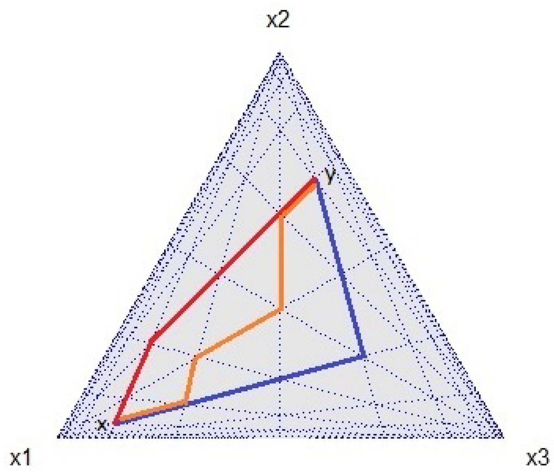
  where $Med(ln\mathbf{x})$ and $Med\left(\mathbf{x}\right)$ are the median of the sets $\{ln{x}_1,\dots ,ln{x}_D\}$ and $\{x_1,\dots ,x_D\}$, respectively. As the logarithm function is strictly increasing, as per Definition 1, the set of points that serve as solutions to the variational problem $T{D}_1$ when applied to log-transformed values ${\mu }_1=\mathit{Med}(ln\left(x\right))$ precisely corresponds to the log-transformed set of points that are solutions to the variational problem $T{D}_1$ when applied to the raw data, that is, $ln\left(\mathit{Med}\right(x\left)\right)$.
  Wu et al. [17] proposed the median of a D-part composition as an alternative denominator to the geometric mean in an attempt to extend the definition of $\mathrm{clr}$-scores. In general, the performance of the median as a robust estimator of the midpoint of a dataset is better when the data have high asymmetry. The CoDa $L^1$-norm captures the distance between two points when movement is restricted to paths that run parallel to the $\mathrm{clr}$-axes ($ln\left(\frac{x_i}{g\left(\mathbf{x}\right)}\right)$), as is the case in a grid or city street network (Manhattan distance, Figure 1). The CoDa $L^1$-norm has an equivalent expression that captures the information about the ratio between the components of a composition; indeed, the median is the central point that divides a set into two equal parts, with half of the values falling below this central position and half above it. Therefore, half of the log-ratios $ln\left(\frac{x_j}{Med\left(\mathbf{x}\right)}\right)$ are positive and the other half are negative. If we rearrange the parts of a composition in increasing order (small to large), i.e., $x_{\left(1\right)}\le \dots \le x_{\left(D\right)}$, then the CoDa $L^1$-norm can be written in the following manner:
  

  Figure 1. The Manhattan distance based on the CoDa $L^1$-norm in the simplex ${\mathit{S}}^3$: the distance between two points $\mathbf{x}=\mathcal{C}\left[e^3,1,e\right]$ and $\mathbf{y}=\mathcal{C}\left[1,e^2,e\right]$ in a grid-based system, where $\mathcal{C}\left[·\right]$ is the closure operation, is represented by three paths (red, orange, and blue) of the same length (five units).

  ∗

  ${\parallel \mathbf{x}\parallel }_{1,{\mathit{S}}^D}=ln\left({\displaystyle \frac{x_{(n+1)}·\dots ·x_{\left(2n\right)}}{x_{\left(1\right)}·\dots ·x_{\left(n\right)}}}\right)$ if $D=2n$;  

  ∗

  ${\parallel \mathbf{x}\parallel }_{1,{\mathit{S}}^D}=ln\left({\displaystyle \frac{x_{(n+1)}·\dots ·x_{(2n-1)}}{x_{\left(1\right)}·\dots ·x_{(n-1)}}}\right)$ if $D=2n-1$.

  Thus, the CoDa $L^1$-norm is a balance between the large parts and small parts.
• The CoDa $L^2$-norm on ${\mathit{S}}^D$ is

  $${\parallel \mathbf{x}\parallel }_{2,{\mathit{S}}^D}=\parallel ln\mathbf{x}-\overline{ln\left(\mathbf{x}\right)}{\mathbf{1}}_D{\parallel }_2={\parallel ln\mathbf{x}-ln\left(g\right(\mathbf{x}\left)\right){\mathbf{1}}_D\parallel }_2={∥ln\frac{\mathbf{x}}{g\left(\mathbf{x}\right)}∥}_2={\left(\sum _{j=1}^D{\left(ln\frac{x_j}{g\left(\mathbf{x}\right)}\right)}^2\right)}^{\frac{1}{2}},$$

  where $g\left(\mathbf{x}\right)$ is the geometric mean of the set $\{x_1,\dots ,x_D\}$. Because $ln\frac{\mathbf{x}}{g\left(\mathbf{x}\right)}\in \mathrm{clr}$-subspace, the CoDa $L^2$-norm is the restricted Euclidean $L^2$-norm on the $\mathrm{clr}$-subspace. This norm is commonly referred to as Aitchison’s norm ${\parallel \mathbf{x}\parallel }_{\mathcal{A}}$ [18].
• The CoDa $L^{\infty }$-norm on ${\mathit{S}}^D$ is

  $${\displaystyle {\parallel \mathbf{x}\parallel }_{\infty ,{\mathit{S}}^D}={\parallel ln\mathbf{x}-MR(ln\mathbf{x}){\mathbf{1}}_D\parallel }_{\infty }={∥ln\frac{\mathbf{x}}{GR\left(\mathbf{x}\right)}∥}_{\infty }=\underset{j}{max}\left\{|ln\frac{x_j}{GR\left(\mathbf{x}\right)}|\right\},}$$

  where $MR(ln\mathbf{x})$ and $GR\left(\mathbf{x}\right)$ are respectively the mid-range and geometric mid-range of the sets $\{ln{x}_1,\dots ,ln{x}_D\}$ and $\{x_1,\dots ,x_D\}$. Note that $MR(ln(\mathbf{x}\left)\right)=ln\left(GR\right(\mathbf{x}\left)\right)$; thus, $GR\left(\mathbf{x}\right)={\left({\displaystyle \underset{i}{max}\left\{x_i\right\}·\underset{j}{min}\left\{x_j\right\}}\right)}^{\frac{1}{2}},i,j=1,\dots ,D$. The CoDa $L^{\infty }$-norm can be interpreted as a form of log-pairwise, as the CoDa $L^{\infty }$-norm represents half of the log-pairwise between the largest part against the smallest part. This log-pairwise is the greatest among all log-pairwise in the composition:

  $${\displaystyle {\parallel \mathbf{x}\parallel }_{\infty ,{\mathit{S}}^D}={\displaystyle \frac{1}{2}}ln\left({\displaystyle \frac{{\displaystyle \underset{i}{max}\left\{x_i\right\}}}{{\displaystyle \underset{j}{min}\left\{x_j\right\}}}}\right)={\displaystyle \frac{1}{2}}\underset{i,j}{max}\left\{ln{\displaystyle \frac{x_i}{x_j}}\right\}.}$$

4. Penalised Regression with a Compositional Covariate

The LASSO regression model is formulated as the combination of the $L^2$-norm cost function and the $L^1$-norm regularisation term [1]. For a real dataset $\mathbf{Z}$ with n observations and D predictors along with a real response vector $\mathbf{Y}$ of length n, the LASSO regression model can be formulated as follows:

$$min\left\{{\displaystyle \frac{1}{2}}\parallel \mathbf{Y}-{\beta }_0-{⟨\mathit{\beta },\mathbf{Z}⟩}_E{\parallel }_2^2+\lambda {\parallel \mathit{\beta }\parallel }_1\right\}$$

(5)

where ${\beta }_0$ is the intercept, the vector $\mathit{\beta }$ is the gradient, and $\lambda$ is the penalty parameter that controls the amount of regularisation. Note that ${\parallel ·\parallel }_2$ and ${\parallel ·\parallel }_1$ refer to the Euclidean $L^2$ and $L^1$ norms in real space, respectively. For $\lambda =0$, the LASSO regression model (Equation (5)) provides the classical least squares regression model. The larger the value of $\lambda$, the greater the number of coefficients in $\mathit{\beta }$ that is forced to be zero. The optimal value of $\lambda$ can be chosen based on cross-validation techniques and related methods [19].

In the case of CoDa, additional considerations must be taken into account in order to respect the compositional nature of both the covariate $\mathbf{X}$ and the intercept $\mathit{\beta }$. In variable selection, [3,20] wrote the LASSO model in terms of ${\mathit{\beta }}^{*}=ln\mathit{\beta }$ and the log-transformed data instead of the $\mathrm{clr}$-scores; consequently, a linear constraint on the compositional gradient coefficient ${\mathit{\beta }}^{*}$ is necessary:

$$min\left\{{\displaystyle \frac{1}{2}}\parallel \mathbf{Y}-{\beta }_0-{⟨{\mathit{\beta }}^{*},ln\left(\mathbf{X}\right)⟩}_E{\parallel }_2^2+\lambda {\parallel {\mathit{\beta }}^{*}\parallel }_1\right\},\mathrm{subject}\mathrm{to}\sum _{j=1}^D{\beta }_j^{*}=0.$$

(6)

Most of the literature addressing the topic of penalised regression with a compositional covariate has predominantly employed the Euclidean $L^1$-norm in the penalty term, leading to a $\mathrm{clr}$-variable selection ([3,4,5,6,20,21,22]).

In Equation (6), the constraint ${\sum }_{j=1}^D{\beta }_j^{*}=0$ can be incorporated in the minimising function. The constraint ${\sum }_{j=1}^D{\beta }_j^{*}=0$ forces the ${\mathit{\beta }}^{*}$ parameter to be an element in the $\mathrm{clr}$-subspace. Therefore, per Equation (4), the inner product ${⟨{\mathit{\beta }}^{*},ln\left(\mathbf{X}\right)⟩}_E$ is equivalent to ${⟨\mathrm{clr}\left(\mathit{\beta }\right),\mathrm{clr}\left(\mathbf{X}\right)⟩}_E={⟨\mathit{\beta },\mathbf{X}⟩}_{\mathcal{A}}$. Thus, the constrained LASSO (Equation (6)) is equivalent to the following definition.

Definition 4. 

Given $y_i$, $i=1,\dots ,n$, the sample of the response variable $\mathbf{X}$, and the $n\times D$ matrix whose rows ${\mathbf{X}}_i=(x_{i1},\dots ,x_{iD})$ for $i=1,\dots ,n$ contain the compositional sample, the $L^1$-$\mathrm{clr}$ LASSO estimator is defined as

$$\mathit{\beta }\in \underset{{\beta }_0,\mathit{\beta }}{argmin}\left\{{\displaystyle \frac{1}{2}}{\parallel \mathbf{Y}-{\beta }_0-{⟨\mathit{\beta },\mathbf{X}⟩}_{\mathcal{A}}\parallel }_2^2+\lambda {\parallel \mathit{\beta }\parallel }_{1-clr}\right\},$$

(7)

where ${\parallel \mathit{\beta }\parallel }_{1-clr}={\sum }_{j=1}^D\left|\mathrm{clr}{\left(\mathit{\beta }\right)}_j\right|={\sum }_{j=1}^D\left|ln\frac{{\beta }_j}{g\left(\mathit{\beta }\right)}\right|.$

The key innovation here is that the linear constraint becomes embedded in the penalty term through the $L^1$-$\mathrm{clr}$ norm. This change in approach is not merely an algebraic or formal change; rather it implies a deeper understanding of the variable selection process in CoDa. The penalty term imposes a constraint on the sum of the absolute values of $\mathrm{clr}$-scores within the gradient vector $\mathit{\beta }$. This constraint compels the model to shrink or eliminate certain $\mathrm{clr}$-scores, effectively driving them to zero. Consequently, this results in a balance selection. Without loss of generality, let us assume that the balance $ln\frac{{\beta }_1}{g\left(\mathit{\beta }\right)}$ is zero. This implies that the corresponding balance $ln\frac{x_1}{g\left(\mathbf{x}\right)}$ has no influence on the response variable y. Therefore, the maximum variation in y is concentrated in the subspace orthogonal to the balance $ln\frac{x_1}{g\left(\mathbf{x}\right)}$, i.e., the subspace of balances among the subcomposition $(x_2,\dots ,x_D)$. This selective regularization process facilitates variable selection, as $x_1$ does not influence the response variable y.

In order to establish a unified framework, the generalised LASSO problem [23] can be adapted to penalised linear models with a compositional covariate:

$$min\left\{{\displaystyle \frac{1}{2}}\parallel \mathbf{Y}-{\beta }_0-{⟨{\mathit{\beta }}^{*},\mathrm{clr}\left(\mathbf{X}\right)⟩}_E{\parallel }_2^2+\lambda {\parallel \mathbf{D}·{\mathit{\beta }}^{*}\parallel }_1\right\},$$

(8)

where ${\parallel ·\parallel }_2$ and ${\parallel ·\parallel }_1$ respectively refer to the Euclidean $L^2$ and $L^1$ norms in real space. The generalised LASSO problem allows for a broader range of applications by considering a matrix $\mathbf{D}$ associated with the penalty term. The matrix $\mathbf{D}$ is related to the $L^1$-norm considered in the penalty term. The choice of one norm over another determines the type of regularization. Different models can be formulated within the framework of the generalised LASSO problem and addressed through convex optimization algorithms. Solving each of these different penalised regression models yields distinct coefficients, each characterised by unique properties. Indeed, Definition 4 can be expressed as a generalised LASSO problem in the following manner:

$${\mathit{\beta }}^{*}\in \underset{{\beta }_0,{\mathit{\beta }}^{*}}{argmin}\left\{{\displaystyle \frac{1}{2}}\sum _{i=1}^n{\left(y_i-{\beta }_0-{⟨{\mathit{\beta }}^{*},\mathrm{clr}{\left(\mathbf{X}\right)}_i⟩}_E\right)}^2+\lambda {\parallel {\mathbf{C}}_D{\mathit{\beta }}^{*}\parallel }_1\right\},$$

(9)

where ${\mathit{\beta }}^{*}=ln\mathit{\beta }$ and $\mathbf{D}={\mathbf{C}}_D$ is the centering matrix on the $\mathrm{clr}$-subspace, with ${\mathbf{C}}_D{\mathit{\beta }}^{*}={\mathit{\beta }}^{*}-\overline{{\mathit{\beta }}^{*}}{\mathbf{1}}_D$.

On the other hand, following [7], it is possible to consider the matrix $\mathbf{D}$ equal to $\mathbf{F}$, that is, the matrix associated with the linear transformation $F({\beta }_1^{*},\dots ,{\beta }_D^{*})={\displaystyle \frac{1}{D-1}}({\beta }_1^{*}-{\beta }_2^{*},{\beta }_1^{*}-{\beta }_3^{*},\dots ,{\beta }_1^{*}-{\beta }_D^{*},{\beta }_2^{*}-{\beta }_3^{*},\dots ,{\beta }_2^{*}-{\beta }_D^{*},\dots ,{\beta }_{D-1}^{*}-{\beta }_D^{*})$. Note that ${\beta }_i^{*}-{\beta }_j^{*}=ln\left(\frac{{\beta }_i}{{\beta }_j}\right)$, which is a log-pairwise. In this case, the penalty term in a generalised LASSO problem can be written as ${\parallel \mathbf{F}·{\mathit{\beta }}^{*}\parallel }_1$, meaning that the generalised LASSO problem results in the following:

$${\mathit{\beta }}^{*}\in \underset{{\beta }_0,{\mathit{\beta }}^{*}}{argmin}\left\{{\displaystyle \frac{1}{2}}\sum _{i=1}^n{\left(y_i-{\beta }_0-{⟨{\mathit{\beta }}^{*},\mathrm{clr}{\left(\mathbf{X}\right)}_i⟩}_E\right)}^2+\lambda {\parallel \mathbf{F}{\mathit{\beta }}^{*}\parallel }_1\right\}.$$

(10)

The model can be defined as follows.

Definition 5. 

Given $y_i$, $i=1,\dots ,n$, the sample of the response variable $\mathbf{X}$, and the $n\times D$ matrix whose rows, ${\mathbf{X}}_i=(x_{i1},\dots ,x_{iD})$ for $i=1,\dots ,n$ contain the compositional sample, the $L^1$-plr LASSO estimator is defined as

$$\mathit{\beta }\in \underset{{\beta }_0,\mathit{\beta }}{argmin}\left\{{\displaystyle \frac{1}{2}}\parallel \mathbf{Y}-{\beta }_0-⟨\mathit{\beta },\mathbf{X}){{⟩}_{\mathcal{A}}\parallel }_2^2+\lambda {\parallel \mathit{\beta }\parallel }_{1-plr}\right\},$$

(11)

where ${\parallel \mathit{\beta }\parallel }_{1-plr}=\frac{1}{D-1}{\sum }_{i<j}\left|ln\left(\frac{{\beta }_i}{{\beta }_j}\right)\right|.$

Importantly, because $ln\frac{{\beta }_i}{{\beta }_j}=\mathrm{clr}{\left(\mathit{\beta }\right)}_i-\mathrm{clr}{\left(\mathit{\beta }\right)}_j$, the penalty term shrinks the absolute value of the differences of the $\mathrm{clr}$-scores within the gradient vector, which forces some pairwise differences of $\mathrm{clr}$-scores to be zero, i.e., it forces equality on some $\mathrm{clr}$-scores. Therefore, each set of equal $\mathrm{clr}$-scores defines a subcomposition with non-influential balances within its parts. This selective regularization process facilitates balanced selection [7].

Finally, using the CoDa $L^1$-norm introduced in Section 3, it is possible to define another generalised LASSO problem.

Definition 6. 

Given $y_i$, $i=1,\dots ,n$, the sample of the response variable $\mathbf{X}$, and the $n\times D$ matrix whose rows ${\mathbf{X}}_i=(x_{i1},\dots ,x_{iD})$ for $i=1,\dots ,n$ contain the compositional sample, the CoDa $L^1$-norm LASSO estimator is defined as

$$\mathit{\beta }\in \underset{{\beta }_0,\mathit{\beta }}{argmin}\left\{{\displaystyle \frac{1}{2}}\parallel \mathbf{Y}-{\beta }_0-⟨\mathit{\beta },\mathbf{X}){{⟩}_{\mathcal{A}}\parallel }_2^2+\lambda {\parallel \mathit{\beta }\parallel }_{1,{\mathit{S}}^D}\right\},$$

(12)

where ${\parallel \mathit{\beta }\parallel }_{1,{\mathit{S}}^D}={\sum }_{j=1}^D\left|ln\frac{{\beta }_j}{Med\left(\mathit{\beta }\right)}\right|.$

In this case, the penalty term compels certain parts ${\beta }_j$ to be equal to the median of the parts, ensuring equality among them in particular. Consequently, the effect produced is also a balance selection, as in the previous case; however, unlike the $L^1$-plr LASSO estimator, with the CoDa $L^1$-norm estimator there is only one set of equal $\mathrm{clr}$-scores, and all non-influential balances belong to a single subcomposition.

As there is no algebraic formula to express the median, $Med\left(\mathit{\beta }\right)$, it is necessary to include a new variable $m\in \mathbb{R}$ in the penalty term when formulating the minimization problem (Equation (12)) as a generalised LASSO problem:

$${\mathit{\beta }}^{*}\in \underset{{\beta }_0,{\mathit{\beta }}^{*},m}{argmin}\left\{{\displaystyle \frac{1}{2}}\sum _{i=1}^n{\left(y_i-{\beta }_0-{⟨{\mathit{\beta }}^{*},\mathrm{clr}{\left(\mathbf{X}\right)}_i⟩}_E\right)}^2+\lambda {\parallel \mathbf{G}·({\mathit{\beta }}^{*},m)\parallel }_1\right\},$$

(13)

where ${\mathit{\beta }}^{*}=ln\mathit{\beta }$, $\mathbf{D}=\mathbf{G}$, and the matrix associated with the transformation $G({\mathit{\beta }}^{*},m)=({\mathit{\beta }}_1^{*}-m,{\mathit{\beta }}_2^{*}-m,\dots ,{\mathit{\beta }}_D^{*}-m)$.

5. Study Case

We used the microbial dataset analyzed in [24,25] to compare the different $L^1$-norms in a CoDa LASSO regression problem. The dataset, collected and explained in [24], comprises the compositions of $D=60$ taxa spanning various taxonomic levels (e.g., g for genus, f for family, o for order, and k for kingdom) within a set of $n=$151 individuals. The dependent variable y is an inflammatory parameter, specifically, the levels of soluble CD14 (sCD14 variable) measured for each individual. These data are available in the R package [26]. An individual having a zero value recorded for some parts indicates that certain taxa were not detected. A zero value prevents the application of the log-ratio methodology. Following a more analogous procedure than in [26], the genus Thalassospira, unclassified genus of the class Alphaproteobacteria, and unclassified genus of the family Porphyromonadaceae, all with more than $80\%$ of zeros, were removed. The rest of the zeros recorded in the remaining 57 taxa were replaced by a small value using an imputation method [27,28]. Because the zeros are of count type, it is appropriate to apply methods based on Dirichlet-multinomial duality [29].

To solve the convex optimizations problems in Equations (9), (10), and (13), we first select the optimal $\lambda$ parameter for the penalised model by performing a ten-fold cross-validation. Each iteration involves dividing the data into ten equal parts, training the model on nine of them, and then evaluating it on the remaining part to produce the lowest Mean Squared Error (MSE). With the parameter $\lambda$ selected, we proceeded to solve the optimization problem in order to find the parameters ${\beta }_0$ and ${\mathit{\beta }}^{*}$. The CVXR package in R version 4.3.2 [30] offers an interface for defining and solving convex optimization problems. CVXR utilises a domain-specific language, making it user-friendly and allowing users to express optimization problems. The package supports various solvers, enabling users to choose the one that best suits their needs. In our case, we opted for the Operator Splitting Quadratic Program (OSQP). The OSQP is a solver for quadratic programming problems and employs an operator-splitting method [31]. This solver is highly efficient even in cases where the matrices are not full-rank, such as our situation, because the $\mathrm{clr}$-scores are used. Referring to the procedure detailed above, we have outlined an Algorithm 1 for a generalised LASSO method below.

The algorithm is applied in the three cases discussed in the previous section, namely, when considering the three different $L^1$ norms in the penalty term, i.e., the $L^1$-$\mathrm{clr}$ (Definition 4), $L^1$-plr (Definition 5), and CoDa $L^1$-norms (Definition 6).

For the $L^1$-$\mathrm{clr}$ estimator, the LASSO regression algorithm is applied iteratively within the cross-validation framework. Figure 2 illustrates the cross-validated MSE across different $\lambda$ values. The optimal $\lambda$ is determined by selecting the point on the curve where the mean squared error is minimised: ${\lambda }_{min}$ = 35,769.42.

Algorithm 1 Generalised LASSO for CoDa

1. Fit the generalised LASSO model with tuning parameter $\lambda$ (Equations (9), (10) or (13)). 2. Calculate the $\mathrm{clr}$-representative: ${\mathit{\beta }}^{*}-\overline{{\mathit{\beta }}^{*}}$ 3. Express the generalised LASSO model in terms of $\mathrm{clr}$-scores.

Figure 2. $L^1$-$\mathrm{clr}$: cross-validation MSE curve for different log-transformed values of the penalty parameter ($ln\left(\lambda \right)$). The circle (∘) is the arithmetical mean of the ten-fold CV. The red lines (above and below the mean) indicate the mean ± stdev value, where stdev is the standard deviation of the ten-fold CV. The vertical line represents the log-transformed values of lambda.min = 35,769.42.

For ${\lambda }_{min}$ = 35,769.42, the generalised LASSO (Equation (9)) identifies which ones among all the ${\beta }_i^{*}$ are set to $\overline{{\beta }^{*}}$, particularly ensuring equality among them. Importantly, when computing the representative ${\beta }^{*}-\overline{{\beta }^{*}}{\mathbf{1}}_D\in \mathrm{clr}$-subspace, we find that some $\mathrm{clr}$-scores are equal to zero. Therefore, the regularization process effectively splits the composition into two subcompositions. The first subcomposition represents the 33 non-influential parts, where coefficients $\mathrm{clr}{\left(\mathit{\beta }\right)}_k,k=1,\dots ,33$ are driven to zero, contributing to model simplicity. The second subcomposition identifies the 24 parts that actively contribute to the influential balances on the response variable y (see Table A1). The intercept ${\beta }_0$ is equal to $6563.19$. Figure 3a shows the non-zero $\mathrm{clr}$-scores for parameter $\mathit{\beta }$. We highlight that the most influential pairwise is formed by the genus Subdoligranulum and the unclassified genus of the family Lachnospiraceae.

Figure 3. Comparison of the $\mathrm{clr}\left(\mathit{\beta }\right)$ parameter, with the taxon order maintained on the vertical axis to facilitate comparison: (a) $\mathrm{clr}$-scores for the $L^1$-$\mathrm{clr}$ LASSO estimator, (b) $\mathrm{clr}$-scores for the $L^1$-CoDa LASSO estimator, and (c) $\mathrm{clr}$-scores for the $L^1$-plr LASSO estimator.

For the CoDa $L^1$-norm estimator (Equation (13)), the LASSO regression algorithm is applied with the same cross-validation partition used in the $L^1$-$\mathrm{clr}$ estimator. Figure 4 illustrates the model’s performance across different regularization parameters $\lambda$. The optimal value is ${\lambda }_{min}$ = 45,582.21

Figure 4. CoDa $L^1$-norm: cross-validation MSE curve for different log-transformed values of the penalty parameter ($ln\left(\lambda \right)$). The circle (∘) is the arithmetical mean of the ten-fold CV. The red lines (above and below the mean) represent the value mean ± stdev, where stdev is the standard deviation of the ten-fold CV. The vertical line represents the log-transformed values of lambda.min = 45,582.21.

For ${\lambda }_{min}$ = 45,582.21, the generalised LASSO (Equation (13)) identifies which ones among all the ${\beta }_i^{*}$ are set to the median of ${\mathit{\beta }}^{*}$, particularly ensuring equality among them. This equality among some ${\mathit{\beta }}_i^{*}$ indicates that the balances involving their respective parts $x_i$ have a non-influential role in the response variable y. However, in contrast to the $L^1$-$\mathrm{clr}$ scenario when computing the representative ${\mathit{\beta }}^{*}-\overline{{\mathit{\beta }}^{*}}$, in general, all $\mathrm{clr}$-scores are non-zero. Consequently, variable selection cannot be performed in this case. The regularization process effectively splits the composition into two subcompositions. The first subcomposition represents the 36 internally independent parts, that is, a subcomposition in which the balances between the respective parts do not influence y [32]. The coefficients $\mathrm{clr}{\left(\mathit{\beta }\right)}_k,k=1,\dots ,36$ are driven to the median of ${\mathit{\beta }}^{*}$ ($6.44$), contributing to model simplicity. The second subcomposition identifies the 21 parts that actively contribute to the influential balances on the response variable y (see Table A1).

To highlight the model’s simplicity, it is crucial to accurately summarise the information contained in the first subcomposition. Without loss of generality, let $(x_1,\dots ,x_k)$ be an internally independent subcomposition. The linear model in $\mathrm{clr}$-scores is

$$y={\beta }_0+\sum _{j=1}^k\mathrm{clr}{\left(\beta \right)}_{j}ln{x}_i+\sum _{j=k+1}^D\mathrm{clr}{\left(\beta \right)}_{j}ln{x}_j,\mathrm{clr}{\left(\beta \right)}_1=\dots =\mathrm{clr}{\left(\beta \right)}_k.$$

As explained by [16] in Chapter 4, the best approach to represent a subcomposition is through its geometric mean, denoted as $g_{sub}={(x_1·\dots ·x_k)}^{\frac{1}{k}}$. Therefore, the linear model is

$$y={\beta }_0+k\mathrm{clr}\left({\beta }_{sub}\right)ln{g}_{sub}+\sum _{j=k+1}^D\mathrm{clr}{\left(\beta \right)}_{j}ln{x}_j,$$

where $\mathrm{clr}\left({\beta }_{sub}\right)=\mathrm{clr}{\left(\beta \right)}_1=\dots =\mathrm{clr}{\left(\beta \right)}_k$. This model has $D-k$ degrees of freedom, as opposed to the $D-1$ degrees of freedom of the general linear model. The intercept value is ${\beta }_0=7023.879$, and Figure 3b shows the $\mathrm{clr}$-scores of $\mathit{\beta }$.

$L^1$-$\mathrm{clr}$ regularization creates a subcomposition that is both internally and externally independent [32], that is, both the balances within the parts of the subcomposition and the full balance between the parts of the subcomposition and the rest of the parts are all non-influential. In contrast, CoDa $L^1$-norm regularization relaxes the conditions and establishes only one subcomposition that is internally independent. In this context, the CoDa $L^1$-norm is somewhat more permissive. When comparing the results, we observe that both are quite similar; what stands out is the significance of the new variable $g_{sub}$ in the CoDa $L^1$-norm penalised linear model. $L^1$-$\mathrm{clr}$ regularization eliminates the balance $ln\frac{g_{sub}}{g\left(\mathbf{x}\right)}$ without prior analysis. This observation prompts us to consider that the direct application of $L^1$-$\mathrm{clr}$ regularization might be premature. Furthermore, when dealing with a penalised model, it is always possible to subsequently test the nullity of any parameter [33].

$L^1$-$\mathrm{clr}$ and CoDa $L^1$-norm regularization share the fact that both shrink the difference between ${\beta }_i^{*}$ coefficients and a central measure, respectively, the mean and the median; consequently, each regularization technique generates a unique subcomposition with certain properties related to its influence on the dependent variable y. Because the goal of a CoDa analysis is to describe the subcompositional structure of the data, the use of the $L^1$-$\mathrm{clr}$ and CoDa $L^1$-norms in the penalty term leads to a result that has to be considered as limited. To overcome this limitation, the $L^1$-plr norm enables the construction of more than one internally independent subcomposition, which can better capture the subcompositional structure of the data regarding the variable y [7].

With the same data partition as executed in previous cases, we performed cross-validation to find the optimal lambda value for the $L^1$-plr estimator. The optimal parameter is $\lambda$ = 69,669.31 (Figure 5).

Figure 5. $L^1$-plr: cross-validation MSE curve for different log-transformed values of the penalty parameter ($ln\left(\lambda \right)$). The circle (∘) is the arithmetical mean of the ten-fold CV. The red lines (above and below the mean) represent the value mean ± stdev, where stdev is the standard deviation of the ten-fold CV. The vertical line represents the log-transformed values of lambda.min = 69,669.31.

For $\lambda$ = 69,669.31, the generalised LASSO (Equation (13)) splits the composition into six distinct subcompositions: five internally independent subcompositions on response variable y and one subcomposition comprising 14 parts actively contributing to the influential balances on the response variable y (see Table A1 to compare $L^1$-plr estimator with $L^1$-$\mathrm{clr}$ and $L^1$-CoDa estimators, and Table A2 to explore its subcompositional structure). Each of the five internally independent subcompositions related to y contributes to reducing the dimension of the linear model. This reduction is achieved by substituting each subcomposition with its geometric mean ($g-subcom{p}_k,k=1,\dots ,5$), following the approach outlined in the CoDa $L^1$-norm estimator. The intercept value is ${\beta }_0=7023.879$ and Figure 3c shows the $\mathrm{clr}$-scores of $\mathit{\beta }$.

The $L^1$-plr estimator is the simplest and provides us with the most information about the subcompositional structure of the composition as regards the variable y.

6. Discussion

This paper has rigorously defined CoDa $L^p$-norms, providing a foundation for their application. The specific cases of the CoDa $L^1$, $L^2$, and $L^{\infty }$ norms have been studied, interpreting these metrics in terms of log-ratios to enhance the reader’s understanding. Additionally, a unified treatment of three distinct $L^1$-norms tailored for compositional data has been presented in the context of a generalised LASSO problem. Through a detailed examination of the regularization effects of each norm, we have uncovered valuable insights. The $L^1$-$\mathrm{clr}$ norm is well suited for variable selection, creating a unique subcomposition that is both internally and externally independent. The CoDa $L^1$-norm, on the other hand, emphasises internal independence. Lastly, the $L^1$-plr norm showcases a balance selection effect. Consequently, the $L^1$-plr norm enables more detailed study of the subcompositional structure of the compositional covariate $\mathbf{x}$ in relation to the explained variable y.

In this article, we have expanded the methodological toolkit for performing penalised regression with compositional covariates. For low dimensions, our recommendation is to run penalised regression with the $L^1$-plr norm. However, we cannot ignore that variable selection becomes imperative for higher dimensions. Therefore, we suggest conducting an initial examination using the CoDa $L^1$-norm or $L^1$-plr norm to gain insights into the subcompositional structure. Following this analysis, it is possible to proceed with penalised regression employing the $L^1$-$\mathrm{clr}$ norm.

As part of our future work, we aim to investigate penalised regression models that effectively integrate both the $L^1$-plr and $L^1$-$\mathrm{clr}$ norms into the penalty term. This research is expected to offer deeper insight into the underlying structure of compositional data, allowing for a more thorough understanding. Moreover, our aim is to improve the flexibility of modelling, especially in datasets with high dimensionality. This holistic approach will contribute to advancing the applicability and effectiveness of penalised regression techniques in the context of compositional data analysis.

References

- Tibshirani, R. Regression shrinkage and selection via the lasso. J. R. Stat. Soc. Ser. B 1996, 58, 267–288. [Google Scholar] [CrossRef]
- Aitchison, J. The Statistical Analysis of Compositional Data; Chapman & Hall: London, UK, 1986. [Google Scholar]
- Lin, W.; Shi, R.; Feng, R.; Li, H. Variable selection in regression with compositional covariates. Biometrika 2014, 101, 785–797. [Google Scholar] [CrossRef]
- Shi, P.; Zhang, A.; Li, H. Regression analysis for microbiome compositional data. Ann. Appl. Stat. 2016, 10, 1019–1040. [Google Scholar] [CrossRef]
- Lu, J.; Shi, P.; Li, H. Generalized linear models with linear constraints for microbiome compositional data. Biometrics 2019, 75, 235–244. [Google Scholar] [CrossRef] [PubMed]
- Susin, A.; Wang, Y.; Lê Cao, K.A.; Calle, M.L. Variable selection in microbiome compositional data analysis. NAR Genom. Bioinform. 2020, 2, lqaa029. [Google Scholar] [CrossRef] [PubMed]
- Saperas-Riera, J.; Martín-Fernández, J.; Mateu-Figueras, G. Lasso regression method for a compositional covariate regularised by the norm L1 pairwise logratio. J. Geochem. Explor. 2023, 255, 107327. [Google Scholar] [CrossRef]
- Egozcue, J.J.; Pawlowsky-Glahn, V. Groups of parts and their balances in compositional data analysis. Math. Geol. 2005, 37, 795–828. [Google Scholar] [CrossRef]
- Pawlowsky-Glahn, V.; Egozcue, J.J. Geometric approach to statistical analysis on the simplex. Stoch. Environ. Res. Risk Assess. 2001, 15, 384–398. [Google Scholar] [CrossRef]
- Billheimer, D.; Guttorp, P.; Fagan, W.F. Statistical Interpretation of Species Composition. J. Am. Stat. Assoc. 2001, 96, 1205–1214. [Google Scholar] [CrossRef]
- Aitchison, J.; Bacon-Shone, J. Log contrast models for experiments with mixtures. Biometrika 1984, 71, 323–330. [Google Scholar] [CrossRef]
- Van der Boogaart, K.G.; Tolosana, R. Analyzing Compositional Data with R; Use R! Springer: Berlin/Heidelberg, Germany, 2013. [Google Scholar]
- Dave, A. Measurement of Central Tendency. In Applied Statistics for Economics; Horizon Press: Toronto, ON, Canada, 2014; Chapter 3. [Google Scholar]
- Barceló-Vidal, C.; Martín-Fernández, J.A. The Mathematics of Compositional Analysis. Austrian J. Stat. 2016, 45, 57–71. [Google Scholar] [CrossRef]
- Brezis, H. Functional Analysis, Sobolev Spaces and Partial Differential Equations; Universitext; Springer: New York, NY, USA, 2011. [Google Scholar]
- Pawlowsky-Glahn, V.; Egozcue, J.J.; Tolosana-Delgado, R. Modeling and Analysis of Compositional Data; John Wiley & Sons: Chichester, UK, 2015. [Google Scholar]
- Wu, J.R.; Macklaim, J.M.; Genge, B.L.; Gloor, G.B. Finding the Centre: Compositional Asymmetry in High-Throughput Sequencing Datasets. In Advances in Compositional Data Analisys; Springer: Berlin/Heidelberg, Germany, 2021; Chapter 17; pp. 329–342. [Google Scholar] [CrossRef]
- Martín-Fernández, J. Measures of Difference and Non-Parametric Classification of Compositional Data. Ph.D. Thesis, Department of Applied Mathematics, Universitat Politècnica de Catalunya, Barcelona, Spain, 2001. [Google Scholar]
- James, G.; Witten, D.; Hastie, T.; Tibshirani, R. Introduction to Statistical Learning, 2nd ed.; Springer: New York, NY, USA, 2021. [Google Scholar]
- Bates, S.; Tibshirani, R. Log-ratio lasso: Scalable, sparse estimation for log-ratio models. Biometrics 2019, 75, 613–624. [Google Scholar] [CrossRef]
- Monti, G.; Filzmoser, P. Sparse least trimmed squares regression with compositional covariates for high-dimensional data. Bioinformatics 2021, 37, 3805–3814. [Google Scholar] [CrossRef] [PubMed]
- Monti, G.; Filzmoser, P. Robust logistic zero-sum regression for microbiome compositional data. Adv. Data Anal. Classif. 2022, 16, 301–324. [Google Scholar] [CrossRef]
- Tibshirani, R.; Taylor, J. The solution path of the generalized lasso. Ann. Statist. 2011, 39, 1335–1371. [Google Scholar] [CrossRef]
- Noguera-Julian, M.; Rocafort, M.; Guillén, Y.; Rivera, J.; Casadellà, M.; Nowak, P.; Hildebrand, F.; Zeller, G.; Parera, M.; Bellido, R.; et al. Gut Microbiota Linked to Sexual Preference and HIV Infection. eBioMedicine 2016, 5, 135–146. [Google Scholar] [CrossRef] [PubMed]
- Rivera-Pinto, J.; Egozcue, J.J.; Pawlowsky-Glahn, V.; Paredes, R.; Noguera-Julian, M.; Calle, M.L. Balances: A new perspective for microbiome analysis. mSystems 2018, 3, e00053-18. [Google Scholar] [CrossRef] [PubMed]
- Calle, M.; Susin, T.; Pujolassos, M. coda4microbiome: Compositional Data Analysis for Microbiome Studies; R Package Version 0.2.1. BMC Bioinf. 2023; 24, 82. [Google Scholar]
- Palarea-Albaladejo, J.; Martín-Fernández, J.A. zCompositions—R package for multivariate imputation of left-censored data under a compositional approach. Chemom. Intell. Lab. Syst. 2015, 143, 85–96. [Google Scholar] [CrossRef]
- Palarea-Albaladejo, J.; Martin-Fernandez, J. zCompositions: Treatment of Zeros, Left-Censored and Missing Values in Compositional Data Sets; R Package Version 1.5. 2023. Available online: https://cran.r-project.org/web/packages/zCompositions/zCompositions.pdf (accessed on 13 March 2024).
- Martín-Fernández, J.; Hron, K.; Templ, M.; Filzmoser, P.; Palarea-Albaladejo, J. Bayesian-multiplicative treatment of count zeros in compositional data sets. Stat. Model. 2015, 15, 134–158. [Google Scholar] [CrossRef]
- Fu, A.; Narasimhan, B.; Boyd, S. CVXR: An R Package for Disciplined Convex Optimization. J. Stat. Softw. 2020, 94, 1–34. [Google Scholar] [CrossRef]
- Stellato, B.; Banjac, G.; Goulart, P.; Bemporad, A.; Boyd, S. OSQP: An Operator Splitting Solver for Quadratic Programs. Math. Program. Comput. 2020, 12, 637–672. [Google Scholar] [CrossRef]
- Boogaart, K.; Filzmoser, P.; Hron, K.; Templ, M.; Tolosana-Delgado, R. Classical and robust regression analysis with compositional data. Math. Geosci. 2021, 53, 823–858. [Google Scholar] [CrossRef]
- Hyun, S.; G’Sell, M.; Tibshirani, R.J. Exact post-selection inference for the generalized lasso path. Electron. J. Stat. 2018, 12, 1053–1097. [Google Scholar] [CrossRef]
Disclaimer/Publisher’s Note: The statements, opinions and data contained in all publications are solely those of the individual author(s) and contributor(s) and not of MDPI and/or the editor(s). MDPI and/or the editor(s) disclaim responsibility for any injury to people or property resulting from any ideas, methods, instructions or products referred to in the content. |
© 2024 by the authors. Licensee MDPI, Basel, Switzerland. This article is an open access article distributed under the terms and conditions of the Creative Commons Attribution (CC BY) license (https://creativecommons.org/licenses/by/4.0/).