Numerical Analysis for Sturm–Liouville Problems with Nonlocal Generalized Boundary Conditions

Abstract

For the generalized Sturm–Liouville problem (GSLP), a new formulation is undertaken to reduce the number of unknowns from two to one in the target equation for the determination of eigenvalue. The eigenparameter-dependent shape functions are derived for using in a variable transformation, such that the GSLP becomes an initial value problem for a new variable. For the uniqueness of eigenfunction an extra condition is imposed, which renders the right-end value of the new variable available; a derived implicit nonlinear equation is solved by an iterative method without using the differential; we can achieve highly precise eigenvalues. For the nonlocal Sturm–Liouville problem (NSLP), we consider two types of integral boundary conditions on the right end. For the first type of NSLP we can prove sufficient conditions for the positiveness of the eigenvalue. Negative eigenvalues and multiple solutions may exist for the second type of NSLP. We propose a boundary shape function method, a two-dimensional fixed-quasi-Newton method and a combination of them to solve the NSLP with fast convergence and high accuracy. From the aspect of numerical analysis the initial value problem of ordinary differential equations and scalar nonlinear equations are more easily treated than the original GSLP and NSLP, which is the main novelty of the paper to provide the mathematically equivalent and simpler mediums to determine the eigenvalues and eigenfunctions.

1. Introduction

The Sturm–Liouville problems and their generalizations are important issues in computational mathematics. Let us consider a generalized Sturm–Liouville problem (GSLP):

$$\begin{array}{c}{w}^{″}\left(x\right)+q(x,\lambda )w\left(x\right)=0,0<x<1,\end{array}$$

(1)

$$\begin{array}{c}{\mathcal{L}}_{\lambda }\left(w\right):=a_1\left(\lambda \right)w\left(0\right)+b_1\left(\lambda \right)w^{\prime }\left(0\right)=0,\end{array}$$

(2)

$$\begin{array}{c}{\mathcal{R}}_{\lambda }\left(w\right):=a_2\left(\lambda \right)w\left(1\right)+b_2\left(\lambda \right)w^{\prime }\left(1\right)=0.\end{array}$$

(3)

We seek $\lambda$ and $w\left(x\right)$ by giving $q(x,\lambda )$, $a_1\left(\lambda \right)$, $b_1\left(\lambda \right)$, $a_2\left(\lambda \right)$ and $b_2\left(\lambda \right)$, where $[a_1^2\left(\lambda \right)+b_1^2\left(\lambda \right)][a_2^2\left(\lambda \right)+b_2^2\left(\lambda \right)]>0$. ${\mathcal{L}}_{\lambda }\left(w\right)$ and ${\mathcal{R}}_{\lambda }\left(w\right)$ are, respectively, the left and right linear boundary operators, depending on $\lambda$.

When $q(x,\lambda )=\lambda q_1\left(x\right)+q_2\left(x\right)$ and constant $a_1$, $b_1$, $a_2$ and $b_2$ are given in Equations (1)–(3), we recover to the Sturm–Liouville problem (SLP). It is known that solving the GSLP is more difficult than solving the SLP. Therefore, it is important that for the GSLP one can develop efficient methods [1,2,3,4,5,6,7,8,9].

As a special case of Equations (1)–(3), Aliyev and Kerimov [1] studied the following spectral problem:

$$\begin{array}{c}{w}^{″}\left(x\right)+[\lambda -q\left(x\right)]w\left(x\right)=0,0<x<1,\hfill \end{array}$$

(4)

$$\begin{array}{c}{w}^{\prime }\left(0\right)sin\beta =w\left(0\right)cos\beta ,0\le \beta <\pi ,\hfill \end{array}$$

(5)

$$\begin{array}{c}{w}^{\prime }\left(1\right)=(a{\lambda }^2+b\lambda +c)w\left(1\right),\hfill \end{array}$$

(6)

where $a\ne 0$, b, c and $\beta$ are real constants. In terms of a target function

$$f\left(\lambda \right)=w^{\prime }(1;\lambda )-(a{\lambda }^2+b\lambda +c)w(1;\lambda ),$$

(7)

and root functions system, the authors proved that for the basisness in $L_2$, the part of the root space is quadratically close to systems of sines and cosines. In general, the target function is different from the characteristic function, which is usually not attainable in the closed form. The above work was extended in [10] to a boundary condition linearly dependent on the eigenparameter. In this paper, we also set the target equation $f\left(\lambda \right)=a_2\left(\lambda \right)w(1;\lambda )+b_2\left(\lambda \right)w^{\prime }(1;\lambda )=0$ as a mathematical tool to determine the eigenvalues. However, we emphasize the numerical aspect of the spectral problem of Equations (1)–(3), which is not addressed in [1].

Currently, the Sturm–Liouville problems with eigenparameter-dependent boundary conditions and transmission conditions are also important issues in many studies [11,12]. Recently, many engineering issues and mathematical schemes have been presented resolving the GSLPs, e.g., an analytical method to acquire the sharp estimates for the lowest positive periodic eigenvalue and all Dirichlet eigenvalues of a GSLP [13]; a class of generalized discontinuous GSLPs with boundary conditions rationally dependent on the eigenparameter was solved by using operator theoretic formulation under the new inner product [14]; the GSLP had infinite eigenvalues and corresponding eigenfunctions existed such that the sequence of eigenvalues was increasing as shown in [15]; a thorough formulation of the weighted residual collocation method was based on the Bernstein polynomials for a class of Sturm–Liouville boundary value problems [16]; the infinitely dimensional minimization problem of the lowest positive Neumann eigenvalue for the SLP [17], and an optimal design of a structure was described by a GSLP with a spectral parameter in the boundary conditions [18].

The integral type nonlocal boundary conditions (BCs) are an area of the fast-developing differential equations theory, which may rise up when the solution on the boundary is connected with the values inside the domain. There are some works on the forced Duffing equation with integral boundary conditions [19,20,21,22], which are effective methods for solving the boundary value problem (BVP) with linear integral BCs [22,23,24].

As defined in [25], the boundary shape function (BSF) automatically satisfies the BCs, which includes the solution of BVP as a special member since the solution must exactly satisfy the specified BCs. The boundary shape function method (BSFM) has been adopted to solve some BVPs [25] with conventional local BCs. Recently, Liu [26] provided a unified BSFM to resolve the eigenvalue problems of SLP, GSLP and periodic SLP. However, the method based on the BSF is not yet developed for solving the NSLP endowed with nonlocal BCs. The SLP with nonlocal BCs has been investigated in [27,28,29,30,31], and has been surveyed in [32]. Those papers were mainly focused on theoretical analyses, and the numerical algorithm to solve the NSLP is not addressed.

Sequentially, we construct two $\lambda$-dependent shape functions and a variable transformation for the GSLP in Section 2. In Section 3, an initial value problem for a new variable with the aid of the normalization technique is derived. To match the right-end BC an implicit nonlinear equation is derived to obtain the eigenvalues by an iterative scheme. Five testing examples are revealed in Section 4. In Section 5, we discuss the first type NSLP to prove $\lambda >0$, and develop the boundary shape function method (BSFM) for a new variable to iteratively solve the eigenvalue, wherein two examples are given. In Section 6, the second type of NSLP is studied and solved iteratively by the BSFM for a new variable. Two examples are given to display the multiple solutions. To obtain the eigenvalue precisely, we develop a two-dimensional fixed-quasi-Newton method (FQNM) in Section 7 for solving the first type NSLP in the original variable, and the second type NSLP in the new variable. The conclusions are drawn in Section 8.

2. Boundary Shape Function

We explore a novel method in [33] for solving a nonlinear equation, which is combined to the boundary shape function method [25] to solve Equations (1)–(3). For this purpose we need to develop a new mathematical method for transforming Equations (1)–(3) to an initial value problem with a new idea of the eigenparameter-dependent boundary shape function.

Let $s_1(x,\lambda )$ and $s_2(x,\lambda )$ be shape functions of x and $\lambda$:

$$\begin{array}{c}{\mathcal{L}}_{\lambda }\left(s_1\right)=a_1\left(\lambda \right)s_1(0,\lambda )+b_1\left(\lambda \right)s_1^{\prime }(0,\lambda )=1,{\mathcal{R}}_{\lambda }\left(s_1\right)=a_2\left(\lambda \right)s_1(1,\lambda )+b_2\left(\lambda \right)s_1^{\prime }(1,\lambda )=0,\hfill \end{array}$$

(8)

$$\begin{array}{c}{\mathcal{L}}_{\lambda }\left(s_2\right)=a_1\left(\lambda \right)s_2(0,\lambda )+b_1\left(\lambda \right)s_2^{\prime }(0,\lambda )=0,{\mathcal{R}}_{\lambda }\left(s_2\right)=a_2\left(\lambda \right)s_2(1,\lambda )+b_2\left(\lambda \right)s_2^{\prime }(1,\lambda )=1.\hfill \end{array}$$

(9)

If $a_1\left(\lambda \right)[a_2\left(\lambda \right)+b_2\left(\lambda \right)]-a_2\left(\lambda \right)b_1\left(\lambda \right)\ne 0$, we can derive

$$s_1(x,\lambda )=\frac{a_2\left(\lambda \right)+b_2\left(\lambda \right)-a_2\left(\lambda \right)x}{a_1\left(\lambda \right)[a_2\left(\lambda \right)+b_2\left(\lambda \right)]-a_2\left(\lambda \right)b_1\left(\lambda \right)},s_2(x,\lambda )=\frac{a_1\left(\lambda \right)x-b_1\left(\lambda \right)}{a_1\left(\lambda \right)[a_2\left(\lambda \right)+b_2\left(\lambda \right)]-a_2\left(\lambda \right)b_1\left(\lambda \right)}.$$

(10)

Theorem 1. 

For any $v\left(x\right)\in {\mathcal{C}}^2[0,1]$, if $s_1(x,\lambda )$ and $s_2(x,\lambda )$ satisfy Equations (8) and (9), then the function $w\left(x\right)$, given by

$$w\left(x\right)=v\left(x\right)-T(x,\lambda ),$$

(11)

 automatically satisfies the boundary conditions (2) and (3), where $T(x,\lambda )$ is given by

$$T(x,\lambda ):=[v\left(0\right)a_1\left(\lambda \right)+v^{\prime }\left(0\right)b_1\left(\lambda \right)]s_1(x,\lambda )+s_2(x,\lambda )[a_2\left(\lambda \right)v\left(1\right)+b_2\left(\lambda \right)v^{\prime }\left(1\right)].$$

(12)

Proof. 

Applying ${\mathcal{L}}_{\lambda }$ to Equation (11), and using the first ones in Equations (8) and (9), we have

$$\begin{array}{c}{\mathcal{L}}_{\lambda }\left(w\right)={\mathcal{L}}_{\lambda }\left(v\right)-{\mathcal{L}}_{\lambda }\left(s_1\right)[v\left(0\right)a_1\left(\lambda \right)+v^{\prime }\left(0\right)b_1\left(\lambda \right)]-{\mathcal{L}}_{\lambda }\left(s_2\right)[a_2\left(\lambda \right)v\left(1\right)+b_2\left(\lambda \right)v^{\prime }\left(1\right)]\hfill \\ =a_1\left(\lambda \right)v\left(0\right)+b_1\left(\lambda \right)v^{\prime }\left(0\right)-[v\left(0\right)a_1\left(\lambda \right)+v^{\prime }\left(0\right)b_1\left(\lambda \right)]=0,\hfill \end{array}$$

where ${\mathcal{L}}_{\lambda }\left(v\right)=a_1\left(\lambda \right)v\left(0\right)+b_1\left(\lambda \right)v^{\prime }\left(0\right)$ was taken into account. Hence, we proved Equation (2).

Similarly, applying ${\mathcal{R}}_{\lambda }$ to Equation (11) and using the second ones in Equations (8) and (9), leads to

$$\begin{array}{c}{\mathcal{R}}_{\lambda }\left(w\right)={\mathcal{R}}_{\lambda }\left(v\right)-{\mathcal{R}}_{\lambda }\left(s_1\right)[v\left(0\right)a_1\left(\lambda \right)+v^{\prime }\left(0\right)b_1\left(\lambda \right)]-{\mathcal{R}}_{\lambda }\left(s_2\right)[a_2\left(\lambda \right)v\left(1\right)+b_2\left(\lambda \right)v^{\prime }\left(1\right)]\hfill \\ =a_2\left(\lambda \right)v\left(1\right)+b_2\left(\lambda \right)v^{\prime }\left(1\right)-[a_2\left(\lambda \right)v\left(1\right)+b_2\left(\lambda \right)v^{\prime }\left(1\right)]=0,\hfill \end{array}$$

where ${\mathcal{R}}_{\lambda }\left(v\right)=a_2\left(\lambda \right)v\left(1\right)+b_2\left(\lambda \right)v^{\prime }\left(1\right)$ was taken into account. Thus, Equation (3) was proven. □

An eigenparameter-dependent boundary shape function is such a function that it satisfies the eigenparameter-dependent boundary conditions in Equations (2) and (3), automatically. Theorem 1 is crucial that the eigenparameter-dependent boundary shape function can be constructed from Equations (11) and (12) easily, with the help of two shape functions $s_1(x,\lambda )$ and $s_2(x,\lambda )$ and a new function $v\left(x\right)$.

3. An Implicit Nonlinear Equation

3.1. A Definite Initial Value Problem

One drawback in Equation (11) is that the right-end values of $v\left(1\right)$ and $v^{\prime }\left(1\right)$ in $a_2\left(\lambda \right)v\left(1\right)+b_2\left(\lambda \right)v^{\prime }\left(1\right)$ appeared in the translation function $T(x,\lambda )$ are themselves unknown values. In this situation the variable transformation in Equation (11) is hard to work in the present form, since there are three unknown values $\lambda$, $v\left(1\right)$ and $v^{\prime }\left(1\right)$ in $T(x,\lambda )$ to be determined; $v\left(0\right)$ and $v^{\prime }\left(0\right)$ in $T(x,\lambda )$ are some given initial values. We can improve this drawback by considering one extra condition in the following two normalization conditions:

$$\begin{array}{c}w\left(0\right)=A_0,\hfill \end{array}$$

(13)

$$\begin{array}{c}{w}^{\prime }\left(0\right)=B_0,\hfill \end{array}$$

(14)

where $A_0$ and $B_0$ are the given nonzero constants. Hence, $w\left(x\right)$ is unique. If the condition $w\left(0\right)=A_0$ is given, we need to specify the value of $B_0$, say $B_0=1$; in contrast, if the condition $w^{\prime }\left(0\right)=B_0$ is given, we need to specify the value of $A_0$, say $A_0=1$. If $a_1\left(\lambda \right)b_1\left(\lambda \right)\ne 0$ in Equation (2), we can adopt $w\left(0\right)=A_0$ or $w^{\prime }\left(0\right)=B_0$ as a normalization condition. In general, we take $A_0=1$ or $B_0=1$.

Theorem 2. 

If $a_1\left(\lambda \right)=0$ and Equation (13) is adopted, then the translation function $T(x,\lambda )$ in Equation (12) reads as

$$T_a(x,\lambda )=v^{\prime }\left(0\right)b_1\left(\lambda \right)s_1(x,\lambda )+\frac{s_2(x,\lambda )}{s_2(0,\lambda )}\{v\left(0\right)-s_1(0,\lambda )v^{\prime }\left(0\right)b_1\left(\lambda \right)-A_0\}.$$

(15)

If $a_1\left(\lambda \right)\ne 0$ and Equation (14) is imposed, then $T(x,\lambda )$ is given by

$$T_b(x,\lambda )=[v\left(0\right)a_1\left(\lambda \right)+v^{\prime }\left(0\right)b_1\left(\lambda \right)]s_1(x,\lambda )+\frac{s_2(x,\lambda )}{s_2^{\prime }(0,\lambda )}\{v^{\prime }\left(0\right)-s_1^{\prime }(0,\lambda )[v\left(0\right)a_1\left(\lambda \right)+v^{\prime }\left(0\right)b_1\left(\lambda \right)]-B_0\}.$$

(16)

Proof. 

Inserting

$$\eta :=a_2\left(\lambda \right)v\left(1\right)+b_2\left(\lambda \right)v^{\prime }\left(1\right)$$

(17)

into Equation (12), renders

$$T(x,\lambda )=[v\left(0\right)a_1\left(\lambda \right)+v^{\prime }\left(0\right)b_1\left(\lambda \right)]s_1(x,\lambda )+\eta s_2(x,\lambda ).$$

(18)

If $a_1\left(\lambda \right)=0$, the analysis can be succeeded as follows. Inserting Equation (18) into Equation (11), taking $x=0$ and using $w\left(0\right)=A_0$, we have

$$\eta =\frac{1}{s_2(0,\lambda )}\{v\left(0\right)-s_1(0,\lambda )[v\left(0\right)a_1\left(\lambda \right)+v^{\prime }\left(0\right)b_1\left(\lambda \right)]-A_0\};$$

(19)

by Equation (10),

$$s_2(0,\lambda )=-\frac{b_1\left(\lambda \right)}{a_1\left(\lambda \right)[a_2\left(\lambda \right)+b_2\left(\lambda \right)]-a_2\left(\lambda \right)b_1\left(\lambda \right)}\ne 0,$$

due to $b_1\left(\lambda \right)\ne 0$ deduced from $a_1\left(\lambda \right)=0$ and $a_1^2\left(\lambda \right)+b_1^2\left(\lambda \right)>0$. Equation (15) is obtained by Equations (19) and (18) with $a_1\left(\lambda \right)=0$.

Alternatively, for the case of $a_1\left(\lambda \right)\ne 0$, we can continue the following analysis. Differentiating Equations (11) and (18) with respect to x, taking $x=0$ and using $w^{\prime }\left(0\right)=B_0$, yields

$$\eta =\frac{1}{s_2^{\prime }(0,\lambda )}\{v^{\prime }\left(0\right)-s_1^{\prime }(0,\lambda )[v\left(0\right)a_1\left(\lambda \right)+v^{\prime }\left(0\right)b_1\left(\lambda \right)]-B_0\};$$

(20)

by Equation (10),

$$s_2^{\prime }(0,\lambda )=\frac{a_1\left(\lambda \right)}{a_1\left(\lambda \right)[a_2\left(\lambda \right)+b_2\left(\lambda \right)]-a_2\left(\lambda \right)b_1\left(\lambda \right)}\ne 0,$$

due to $a_1\left(\lambda \right)\ne 0$. It immediately leads to Equation (16) by inserting Equation (20) for $\eta$ into Equation (18). □

Theorem 2 is interesting that by using the normalization condition the translation function $T(x,\lambda )$ can be reduced to a function that merely involves $\lambda$ as an unknown value. The reduction from three unknown values $\lambda$, $v\left(1\right)$ and $v^{\prime }\left(1\right)$ to one unknown value $\lambda$ is a key point for the success of the iterative algorithm to be presented in Section 3.2.

Theorem 3. 

If $a_1\left(\lambda \right)=0$ and Equation (13) is adopted, then Equations (1)–(3) can be transformed to

$$v^{″}\left(x\right)=T_a^{″}(x,\lambda )-q(x,\lambda )[v\left(x\right)-T_a(x,\lambda )],$$

(21)

 where the new variable $v\left(x\right)$ is subjected to

$$a_2\left(\lambda \right)[v\left(1\right)-T_a(1,\lambda )]+b_2\left(\lambda \right)[v^{\prime }\left(1\right)-T_a^{\prime }(1,\lambda )]=0.$$

(22)

If $a_1\left(\lambda \right)\ne 0$ and Equation (14) is imposed, then Equations (1)–(3) can be transformed to

$$v^{″}\left(x\right)=T_b^{″}(x,\lambda )+q(x,\lambda )[T_b(x,\lambda )-v\left(x\right)],$$

(23)

 which is subjected to 

$$a_2\left(\lambda \right)[v\left(1\right)-T_b(1,\lambda )]+b_2\left(\lambda \right)[v^{\prime }\left(1\right)-T_b^{\prime }(1,\lambda )]=0.$$

(24)

For Equation (21) or Equation (23), $v\left(0\right)=c_1$ and $v^{\prime }\left(0\right)=c_2$ are the specified initial conditions with $c_1$ and $c_2$ given constants.

Proof. 

Inserting $w\left(x\right)=v\left(x\right)-T_a(x,\lambda )$ into Equations (1) and (3), we can derive Equations (21) and (22). Similarly, we can prove Equations (23) and (24). □

Although the proof of Theorem 3 is straightforward, it is very important that we can fully transform Equations (1)–(3) to an initial value problem of the second-order ordinary differential equation (ODE) for the new variable $v\left(x\right)$, and a nonlinear equation as the target equation to determine the eigenvalue $\lambda$.

3.2. An Iterative Algorithm

Liu et al. [33] proposed an iterative scheme (LHL) to find the root of $f\left(x\right)=0$:

$$x_{n+1}=x_n-\frac{f\left(x_n\right)}{a+bf\left(x_n\right)},$$

(25)

where

$$a=f^{\prime }\left(r\right),b=\frac{f^{″}\left(r\right)}{2f^{\prime }\left(r\right)},$$

(26)

with $f\left(r\right)=0$ and $f^{\prime }\left(r\right)\ne 0$. Equation (25) has third-order convergence.

Choose $x_0$ and $x_2$ with $r\in (x_0,x_2)$ to render $f\left(x_0\right)f\left(x_2\right)<0$. Then, we take $x_1=(x_0+x_2)/2$ and approximate a and b in Equation (26) by using the finite differences:

$$a=\frac{f\left(x_2\right)-f\left(x_0\right)}{x_2-x_0},b=\frac{1}{2a}\frac{f\left(x_2\right)-2f\left(x_1\right)+f\left(x_0\right)}{{(x_1-x_0)}^2}.$$

(27)

The procedures for solving $f\left(x\right)=0$ are given as follows: (i) Take $x_0$ and $x_2$ such that $f\left(x_0\right)f\left(x_2\right)<0$. (ii) Obtain a and b by Equation (27). (iii) For $k=0,1,\dots$, iterate

$$x_{k+1}=x_k-\frac{f\left(x_k\right)}{a+bf\left(x_k\right)},$$

(28)

until $\left|f\right(x_k\left)\right|<ϵ$.

The idea to solve Equations (1)–(3) is now simplifying to the shooting method to solve Equations (21) and (22) or Equations (23) and (24). For each given value of $\lambda$ and the given initial values $v\left(0\right)=c_1$ and $v^{\prime }\left(0\right)=c_2$, we can integrate Equation (21) by employing the fourth-order Runge–Kutta method (RK4). At the endpoint $x=1$ of the integration, we can obtain $v\left(1\right)$ and $v^{\prime }\left(1\right)$ which are implicit functions of $\lambda$. Inserting $v\left(1\right)$ and $v^{\prime }\left(1\right)$ into the target Equation (22), an implicit nonlinear equation denoted by $f_a\left(\lambda \right)$ is obtained as follows:

$$f_a\left(\lambda \right):=a_2\left(\lambda \right)[v\left(1\right)-T_a(1,\lambda )]+b_2\left(\lambda \right)[v^{\prime }\left(1\right)-T_a^{\prime }(1,\lambda )]=0.$$

(29)

Similarly, for each given value of $\lambda$, we can integrate Equation (23) with the given initial values $v\left(0\right)=c_1$ and $v^{\prime }\left(0\right)=c_2$ to obtain $v\left(1\right)$ and $v^{\prime }\left(1\right)$; hence, Equation (24) yields the following implicit nonlinear target equation:

$$f_b\left(\lambda \right):=a_2\left(\lambda \right)[v\left(1\right)-T_b(1,\lambda )]+b_2\left(\lambda \right)[v^{\prime }\left(1\right)-T_b^{\prime }(1,\lambda )]=0.$$

(30)

Equation (29) or Equation (30) is an implicit nonlinear equation of $\lambda$, which can be solved by the LHL in Equation (28).

In the GSLP of Equations (1)–(3) there are two unknowns of $\lambda$ and $w\left(0\right)$ (or $w^{\prime }\left(0\right)$). Equations (21)–(24) overcome this difficulty by reducing two unknowns to one unknown for $\lambda$ in Equations (21) and (22) or Equations (23) and (24).

No matter the cases in Equations (21) and (22), or in Equations (23) and (24), we unify them to

$$\begin{array}{c}{v}^{″}\left(x\right)=F(x,v;\lambda ),v\left(0\right)=c_1,v^{\prime }\left(0\right)=c_2,\hfill \end{array}$$

(31)

$$\begin{array}{c}f\left(\lambda \right)=0,\hfill \end{array}$$

(32)

where $f\left(\lambda \right)$ is an implicit function of $\lambda$ through $v(1;\lambda )$ and $v^{\prime }(1;\lambda )$.

The iterative processes for solving Equations (1)–(3) to determine the eigenvalue are given as follows: (i) Give $q(x,\lambda )$, $a_1\left(\lambda \right)$, $b_1\left(\lambda \right)$, $a_2\left(\lambda \right)$, $b_2\left(\lambda \right)$, $c_1$, $c_2$, $ϵ$, $\mathsf{\Delta }x=1/N$, and initial guess ${\lambda }^{\left(0\right)}$. (ii) Give ${\lambda }^0$, ${\lambda }^2$, ${\lambda }^1=({\lambda }^0+{\lambda }^2)/2$; compute Equation (31) by RK4 to obtain $v(1;{\lambda }^0)$ and $v^{\prime }(1;{\lambda }^0)$, and obtain $f\left({\lambda }^0\right)$; compute Equation (31) by RK4 to obtain $v(1;{\lambda }^2)$ and $v^{\prime }(1;{\lambda }^2)$, and obtain $f\left({\lambda }^2\right)$; compute Equation (31) by RK4 to obtain $v(1;{\lambda }^1)$ and $v^{\prime }(1;{\lambda }^1)$, and obtain $f\left({\lambda }^1\right)$; compute

$$a=\frac{f\left({\lambda }^2\right)-f\left({\lambda }^0\right)}{{\lambda }^2-{\lambda }^0},b=\frac{1}{2a}\frac{f\left({\lambda }^2\right)-2f\left({\lambda }^1\right)+f\left({\lambda }^0\right)}{{({\lambda }^1-{\lambda }^0)}^2}.$$

(iii) Conduct $k=0,1,\dots$,

$$\begin{array}{l}\mathrm{compute} \mathrm{Equation} (31) \mathrm{by} \mathrm{RK}4 \mathrm{to} \mathrm{obtain}v(1;{\lambda }^{\left(k\right)}),v^{\prime }(1;{\lambda }^{\left(k\right)}),\\ \mathrm{compute} \mathrm{Equation} (32) \mathrm{to} \mathrm{obtain} f\left({\lambda }^{\left(k\right)}\right),\\ {\lambda }^{(k+1)}={\lambda }^{\left(k\right)}-\frac{f\left({\lambda }^{\left(k\right)}\right)}{a+bf\left({\lambda }^{\left(k\right)}\right)},\end{array}$$

until $|{\lambda }^{(k+1)}-{\lambda }^{\left(k\right)}| <ϵ$.

Because we have mathematically transformed the spectral problem of GSLP to the problem for solving a target equation, the convergence is guaranteed by the LHL with three-order convergence. It is known that the RK4 has fourth-order accuracy which together with the LHL, can achieve highly accurate eigenvalue and the corresponding eigenfunction.

4. Examples Testing

4.1. Example 1

Consider a generalized Sturm–Liouville problem in [1]:

$$\begin{array}{c}{w}^{″}\left(x\right)+\lambda w\left(x\right)=0,0<x<1,\hfill \end{array}$$

(33)

$$\begin{array}{c}{w}^{\prime }\left(0\right)=0,\left(\lambda -\frac{{\lambda }^2}{{\pi }^2}\right)w\left(1\right)+w^{\prime }\left(1\right)=0.\hfill \end{array}$$

(34)

For this problem we solve $\lambda$ from the following characteristic equation in [1]:

$$g\left(\lambda \right)=tan\sqrt{\lambda }-\sqrt{\lambda }\left(1-\frac{\lambda }{{\pi }^2}\right)=0,$$

(35)

which is the explicit form of the characteristic equation and we solve it by using the Newton method. Here $w\left(x\right)=cos\sqrt{\lambda }x$ is the eigenfunction.

As shown in [1], the target equation is

$$f\left(\lambda \right)=\sqrt{\lambda }sin\sqrt{\lambda }-\left(\frac{{\lambda }^2}{{\pi }^2}-\lambda \right)cos\sqrt{\lambda }=0,$$

which can be arranged to Equation (35). For this spectral problem, the target equation is equal to the characteristic equation.

We set $A_0=1$, $N=5000$, $c_1=c_2=0$ and determine $\lambda$ by Equation (29). Table 1 reveals fast convergence with high accuracy for the eigenvalues obtained. NI denotes the number of iterations, the absolute error AE$\left(\lambda \right)$ of eigenvalue, ERBC the absolute error of the right boundary condition, and ME the maximum error of eigenfunction.

Table 1. For example 1, tabulating $\lambda$, $ϵ$, NI, AE$\left(\lambda \right)$, ERBC, and ME.

$\mathit{\lambda }$	$\mathit{ϵ}$	NI	AE (λ)	ERBC	ME
9.86960440101	${10}^{-14}$	12	$2.49 \times {10}^{-14}$	$1.19 \times {10}^{-14}$	$6.89 \times {10}^{-15}$
23.61120532012	${10}^{-15}$	13	$3.52 \times {10}^{-13}$	$1.1 \times {10}^{-13}$	$3.61 \times {10}^{-15}$
199.9633145327	${10}^{-10}$	7	$2.13 \times {10}^{-10}$	$1.12 \times {10}^{-11}$	$7.54 \times {10}^{-12}$

4.2. Example 2

Consider a generalized Sturm–Liouville problem specified in [2,3]:

$$\begin{array}{c}{w}^{″}\left(x\right)+\lambda w\left(x\right)=0,0<x<1,\hfill \end{array}$$

(36)

$$\begin{array}{c}w\left(0\right)+(\lambda -4{\pi }^2)w^{\prime }\left(0\right)=0,w\left(1\right)-\lambda w^{\prime }\left(1\right)=0.\hfill \end{array}$$

(37)

The characteristic equation is derived in [3]:

$$g\left(\lambda \right)=\sqrt{\lambda }(4{\pi }^2-2\lambda )cos\sqrt{\lambda }+sin\sqrt{\lambda }(1+4{\pi }^2{\lambda }^2-{\lambda }^3)=0.$$

(38)

No closed-form eigenfunction exists for this spectral problem. We take $B_0=1$, $N=$ 10,000, $c_1=0$ and $c_2=1$, and iteratively determine $\lambda$ by Equation (30) as shown in Table 2.

Table 2. Tabulating $\lambda$, $ϵ$, NI, AE$\left(\lambda \right)$, and ERBC for example 2.

$\mathit{\lambda }$	$\mathit{ϵ}$	NI	AE (λ)	ERBC
9.73088657821	${10}^{-12}$	5	$3.02 \times {10}^{-14}$	$2.82 \times {10}^{-12}$
88.7633162526	${10}^{-10}$	5	$1.05 \times {10}^{-12}$	$2.83 \times {10}^{-10}$
157.884110439	${10}^{-9}$	4	$6.48 \times {10}^{-12}$	$8.31 \times {10}^{-11}$
246.722352967	${10}^{-9}$	5	$2.49 \times {10}^{-11}$	$4.74 \times {10}^{-9}$
355.293796381	${10}^{-9}$	5	$7.47 \times {10}^{-11}$	$2.42 \times {10}^{-9}$

4.3. Example 3

Taken from [3], we consider the following generalized Sturm–Liouville problem:

$$\begin{array}{c}{w}^{″}\left(x\right)+(\lambda -e^x)w\left(x\right)=0,0<x<1,\hfill \end{array}$$

(39)

$$\begin{array}{c}w\left(0\right)=0,w^{\prime }\left(1\right)cos\sqrt{\lambda }-w\left(1\right)\sqrt{\lambda }sin\sqrt{\lambda }=0.\hfill \end{array}$$

(40)

For this spectral problem we have

$$q=\lambda -e^x,a_1=1,b_1=0,a_2=-\sqrt{\lambda }sin\sqrt{\lambda },b_2=cos\sqrt{\lambda }.$$

(41)

It follows from Equation (10) that

$$s_1\left(x\right)=\frac{a_2+b_2-a_{2}x}{a_2+b_2}=1+\frac{x\sqrt{\lambda }sin\sqrt{\lambda }}{cos\sqrt{\lambda }-\sqrt{\lambda }sin\sqrt{\lambda }},s_2\left(x\right)=\frac{a_{1}x}{a_2+b_2}=\frac{x}{cos\sqrt{\lambda }-\sqrt{\lambda }sin\sqrt{\lambda }}.$$

(42)

Then, in view of Equations (17) and (18), one has

$$\begin{array}{c}\eta =cos\sqrt{\lambda }{v}^{\prime }\left(1\right)-\sqrt{\lambda }sin\sqrt{\lambda }v\left(1\right),\hfill \end{array}$$

(43)

$$\begin{array}{c}T=c_1{s}_1\left(x\right)+\eta s_2\left(x\right).\hfill \end{array}$$

(44)

From Equations (23) and (24) the second-order ordinary differential equation and nonlinear equation are given by

$$\begin{array}{c}{v}^{″}\left(x\right)=F(x,v;\lambda )=(\lambda -e^x)[c_1{s}_1\left(x\right)+\eta s_2\left(x\right)-v\left(x\right)],\hfill \end{array}$$

(45)

$$\begin{array}{c}f\left(\lambda \right)=\sqrt{\lambda }sin\sqrt{\lambda }[c_1{s}_1\left(1\right)+\eta s_2\left(1\right)-v\left(1\right)]+cos\sqrt{\lambda }[v^{\prime }\left(1\right)-T^{\prime }]=0,\hfill \end{array}$$

(46)

where

$$T^{\prime }=c_1{s}_1^{\prime }\left(x\right)+\eta s_2^{\prime }\left(x\right)=\frac{c_1\sqrt{\lambda }sin\sqrt{\lambda }}{cos\sqrt{\lambda }-\sqrt{\lambda }sin\sqrt{\lambda }}+\frac{\eta }{cos\sqrt{\lambda }-\sqrt{\lambda }sin\sqrt{\lambda }}.$$

(47)

Now, the iterative method listed Section 3.2 can be applied to compute the eigenvalues of Equations (39) and (40).

We take $B_0=1$, $N=5000$, $c_1=0$ and $c_2=1$ and iteratively determine $\lambda$ by Equation (46) as shown in Table 3, where the exact eigenvalues are given by [3].

Table 3. Tabulating computed and exact $\lambda$, $ϵ$, NI, and ERBC for example 3.

Computed $\mathit{\lambda }$	Exact $\mathit{\lambda }$	$\mathit{ϵ}$	NI	ERBC
0.929062028579	0.92906202857	${10}^{-15}$	9	0
6.74788117822	6.7478811782	${10}^{-15}$	6	$4.44 \times {10}^{-16}$
16.1245477259	16.1245477258	${10}^{-15}$	8	$3.33 \times {10}^{-16}$
31.2202765051	31.2202765051	${10}^{-15}$	7	$6.11 \times {10}^{-16}$
50.7339278392	50.7339278392	${10}^{-15}$	6	$7.22 \times {10}^{-16}$

4.4. Example 4

Consider a generalized Sturm–Liouville problem in [3]:

$$\begin{array}{c}{w}^{″}\left(x\right)+\lambda w\left(x\right)=0,0<x<1,\hfill \end{array}$$

(48)

$$\begin{array}{c}w\left(0\right)-2w^{\prime }\left(0\right)=0,(1+\sqrt{\lambda })w\left(1\right)+(1-\lambda )w^{\prime }\left(1\right)=0,\hfill \end{array}$$

(49)

whose characteristic equation reads as

$$g\left(\lambda \right)=2cos\sqrt{\lambda }+\frac{sin\sqrt{\lambda }}{\sqrt{\lambda }}+(1-\sqrt{\lambda })(cos\sqrt{\lambda }-2\sqrt{\lambda }sin\sqrt{\lambda })=0.$$

(50)

We take $B_0=1$, $N=$ 10,000, $c_1=0$ and $c_2=1$, and iteratively determine $\lambda$ by Equation (30), as shown in Table 4.

Table 4. For example 4 tabulating $\lambda$, $ϵ$, NI, AE$\left(\lambda \right)$, and ERBC.

$\mathit{\lambda }$	$\mathit{ϵ}$	NI	AE (λ)	ERBC
9.93874341403	${10}^{-14}$	6	$8.88 \times {10}^{-15}$	$7.99 \times {10}^{-14}$
40.0989697328	${10}^{-12}$	5	$2.06 \times {10}^{-13}$	$3.73 \times {10}^{-12}$
89.5876345317	${10}^{-12}$	5	$1.21 \times {10}^{-12}$	$1.08 \times {10}^{-12}$

4.5. Example 5

We compute the eigenvalues of the following generalized Sturm–Liouville problem:

$$\begin{array}{c}{w}^{″}\left(x\right)+\lambda w\left(x\right)=0,0<x<1,\hfill \end{array}$$

(51)

$$\begin{array}{c}(1+4{\pi }^2{\lambda }^2-{\lambda }^3)w\left(0\right)+(2\lambda -4{\pi }^2)w^{\prime }\left(0\right)=0,w\left(1\right)=0,\hfill \end{array}$$

(52)

whose eigenvalues are the same as those in Example 2.

We set $A_0=1$, $N=$ 10,000, $c_1=0$ and $c_2=1.5$ and determine $\lambda$ by Equation (29). As shown in Table 5, the accuracy in the right boundary condition is slightly better than that in Table 2.

Table 5. Tabulating $\lambda$, $ϵ$, NI, AE$\left(\lambda \right)$, and ERBC for example 5.

$\mathit{\lambda }$	$\mathit{ϵ}$	NI	AE (λ)	ERBC
9.73088657821	${10}^{-12}$	14	$3.38 \times {10}^{-14}$	$2.39 \times {10}^{-13}$
88.7633162526	${10}^{-10}$	7	$8.53 \times {10}^{-14}$	$1.61 \times {10}^{-11}$
157.884110439	${10}^{-9}$	6	$8.64 \times {10}^{-12}$	$7.04 \times {10}^{-11}$

5. First Type Nonlocal Sturm–Liouville Problem

In this section we consider a nonlocal Sturm–Liouville problem (NSLP) [34,35]:

$$\begin{array}{c}-y^{″}\left(x\right)+q\left(x\right)y\left(1\right)=\lambda y\left(x\right),x\in (0,1),\hfill \end{array}$$

(53)

$$\begin{array}{c}y\left(0\right)=0,y^{\prime }\left(1\right)-{\int }_0^{1}q\left(x\right)y\left(x\right)dx=0,\hfill \end{array}$$

(54)

where $q\left(x\right)$ is a nonlocal potential. To distinguish the NSLP from the GSLP in Equations (1)–(3), we adopt a different notation $y\left(x\right)$ for the eigenfunction, instead of $w\left(x\right)$.

In terms of a nonlocal linear boundary operator:

$$\mathcal{B}\left(y\right):=y^{\prime }\left(1\right)-{\int }_0^{1}q\left(x\right)y\left(x\right)dx,$$

(55)

Equation (54) is written as

$$y\left(0\right)=0,\mathcal{B}\left(y\right)=0.$$

(56)

We can impose a normalization condition:

$$y^{\prime }\left(0\right)=a_0,$$

(57)

where $a_0\ne 0$ is a given constant.

5.1. The Positiveness of $\lambda$

Theorem 4. 

For Equation (53), the conditions in Equation (54) are sufficient for

$$\lambda >0.$$

(58)

Proof. 

Considering $-y\left(x\right)y^{″}\left(x\right)=-{\left[y\left(x\right)y^{\prime }\left(x\right)\right]}^{\prime }+y^{\prime }{\left(x\right)}^2$, with Equation (53) multiplying by $y\left(x\right)$, and integrating both sides, we have

$$\begin{array}{c}-y^{″}\left(x\right)y\left(x\right)+y\left(1\right)q\left(x\right)y\left(x\right)=\lambda y^2\left(x\right),\hfill \\ -{\int }_0^1{y}^{″}\left(x\right)y\left(x\right)dx+y\left(1\right){\int }_0^{1}q\left(x\right)y\left(x\right)dx=\lambda {\int }_0^1{y}^2\left(x\right)dx,\hfill \\ -{\int }_0^1{\left[y\left(x\right)y^{\prime }\left(x\right)\right]}^{\prime }dx+y\left(1\right){\int }_0^{1}q\left(x\right)y\left(x\right)dx+{\int }_0^1{y}^{\prime }{\left(x\right)}^{2}dx=\lambda {\int }_0^1{y}^2\left(x\right)dx,\hfill \\ y\left(0\right)y^{\prime }\left(0\right)+y\left(1\right)\left[{\int }_0^{1}q\left(x\right)y\left(x\right)dx-y^{\prime }\left(1\right)\right]+{\int }_0^1{y}^{\prime }{\left(x\right)}^{2}dx=\lambda {\int }_0^1{y}^2\left(x\right)dx.\hfill \end{array}$$

(59)

If Equation (54) holds, Equation (59) reduces to

$${\int }_0^1{y}^{\prime }{\left(x\right)}^{2}dx=\lambda {\int }_0^1{y}^2\left(x\right)dx,$$

(60)

which provides a formula to compute

$$\lambda =\frac{{\int }_0^1{y}^{\prime }{\left(x\right)}^{2}dx}{{\int }_0^1{y}^2\left(x\right)dx}>0.$$

(61)

Thus, the proof is completed. □

Equation (61) is somewhat similar to the Rayleigh quotient; however, the Rayleigh quotient in the classical Sturm–Liouville problem includes a potential function $q\left(x\right)$ in the integral term ${\int }_0^{1}q\left(x\right)y^2\left(x\right)dx$ at the numerator. Equation (61) is important for developing a highly precise iterative algorithm in Section 7, where

$$\lambda {\int }_0^1{y}^2\left(x\right)dx-{\int }_0^1{y}^{\prime }{\left(x\right)}^{2}dx=0$$

and the second one in Equation (54) constitute coupled nonlinear equations to determine $\lambda$.

5.2. Boundary Shape Function

Let $p_1\left(x\right)$ and $p_2\left(x\right)$ be

$$\begin{array}{c}{p}_1\left(0\right)=1,\mathcal{B}\left(p_1\right)=p_1^{\prime }\left(1\right)-{\int }_0^{1}q\left(x\right)p_1\left(x\right)dx=0,\hfill \end{array}$$

(62)

$$\begin{array}{c}{p}_2\left(0\right)=0,\mathcal{B}\left(p_2\right)=p_2^{\prime }\left(1\right)-{\int }_0^{1}q\left(x\right)p_2\left(x\right)dx=1.\hfill \end{array}$$

(63)

We can derive

$$p_1\left(x\right)=1+\frac{x{\int }_0^{1}q\left(x\right)dx}{1-{\int }_0^{1}xq\left(x\right)dx},p_2\left(x\right)=\frac{x}{1-{\int }_0^{1}xq\left(x\right)dx},$$

(64)

where we suppose that $1-{\int }_0^{1}xq\left(x\right)dx\ne 0$.

Theorem 5. 

For any $u\left(x\right)\in {\mathcal{C}}^2[0,1]$, if $p_1\left(x\right)$ and $p_2\left(x\right)$ satisfy Equations (62) and (63), then the function $y\left(x\right)$ satisfying Equation (54) is given by

$$y\left(x\right)=u\left(x\right)-G\left(x\right),$$

(65)

where 

$$G\left(x\right)=p_1\left(x\right)u\left(0\right)+p_2\left(x\right)\left[u^{\prime }\left(1\right)-{\int }_0^{1}q\left(x\right)u\left(x\right)dx\right].$$

(66)

Proof. 

Inserting $x=0$ into Equation (65) and using $p_1\left(0\right)=1$ and $p_2\left(0\right)=0$, it is apparent that

$$y\left(0\right)=u\left(0\right)-G\left(0\right)=u\left(0\right)-p_1\left(0\right)u\left(0\right)-p_2\left(0\right)\left[u^{\prime }\left(1\right)-{\int }_0^{1}q\left(x\right)u\left(x\right)dx\right]=u\left(0\right)-u\left(0\right)=0.$$

(67)

The first condition in Equation (54) is proven. Applying the linear operator $\mathcal{B}$ to Equation (65), and using the second ones in Equations (62) and (63), we have

$$\begin{array}{c}\mathcal{B}\left(y\right)=\mathcal{B}\left(u\right)-\mathcal{B}\left(p_1\right)u\left(0\right)-\mathcal{B}\left(p_2\right)\left[u^{\prime }\left(1\right)-{\int }_0^{1}q\left(x\right)u\left(x\right)dx\right]\hfill \\ =u^{\prime }\left(1\right)-{\int }_0^{1}q\left(x\right)u\left(x\right)dx-\left[u^{\prime }\left(1\right)-{\int }_0^{1}q\left(x\right)u\left(x\right)dx\right]=0,\hfill \end{array}$$

where $\mathcal{B}\left(u\right)=u^{\prime }\left(1\right)-{\int }_0^{1}q\left(x\right)u\left(x\right)dx$ is taken as that defined in Equation (55). Hence, the second condition in Equation (54) is proven. □

Theorem 5 is critical such that the nonlocal boundary conditions in Equation (54) can be automatically satisfied for $y\left(x\right)$ with the help of two nonlocal shape functions $p_1\left(x\right)$ and $p_2\left(x\right)$ and a new function $u\left(x\right)$.

5.3. Numerical Algorithm

Let

$$b_0:=u^{\prime }\left(1\right)-{\int }_0^{1}q\left(x\right)u\left(x\right)dx;$$

(68)

hence, the variable transformation in Equation (65) reads as

$$y\left(x\right)=u\left(x\right)-p_1\left(x\right)u\left(0\right)-b_0{p}_2\left(x\right).$$

(69)

Following Equation (53), a new second-order ODE for $u\left(x\right)$:

$$-u^{″}\left(x\right)+q\left(x\right)[u\left(1\right)-p_1\left(1\right)u\left(0\right)-b_0{p}_2\left(1\right)]=\lambda [u\left(x\right)-p_1\left(x\right)u\left(0\right)-b_0{p}_2\left(x\right)],$$

(70)

where

$$b_0=\frac{u^{\prime }\left(0\right)-p_1^{\prime }\left(0\right)u\left(0\right)-a_0}{p_2^{\prime }\left(0\right)}$$

(71)

is derived by inserting $x=0$ into the differential of Equation (69) and by using Equation (57). In view of Equation (64),

$$p_2^{\prime }\left(0\right)=\frac{1}{1-{\int }_0^{1}xq\left(x\right)dx}\ne 0,$$

according to the assumption $1-{\int }_0^{1}xq\left(x\right)dx\ne 0$; hence, $b_0$ is a well-defined constant given in Equation (71).

In terms of $u\left(x\right)$, $\lambda$ in Equation (61) is recast to

$$\lambda =\frac{{\int }_0^1{[u^{\prime }\left(x\right)-p_1^{\prime }\left(x\right)u\left(0\right)-b_0{p}_2^{\prime }\left(x\right)]}^{2}dx}{{\int }_0^1{[u\left(x\right)-p_1\left(x\right)u\left(0\right)-b_0{p}_2\left(x\right)]}^{2}dx}.$$

(72)

Let $u_1\left(x\right)=u\left(x\right)$, $u_2\left(x\right)=u^{\prime }\left(x\right)$, $u_1\left(0\right)=u\left(0\right)=c_1$, $u_2\left(0\right)=u^{\prime }\left(0\right)=c_2$ and $\alpha =u_1\left(1\right)=u\left(1\right)$, which is an unknown constant. For solving Equations (53) and (54), we list the iterative algorithm based on the boundary shape function method (BSFM). (i) Give $q\left(x\right)$ and derive $p_1\left(x\right)$ and $p_2\left(x\right)$; give $c_1$, $c_2$, $a_0$, initial guesses of ${\lambda }_0$, ${\alpha }_0$, $ϵ$ and N. (ii) Calculate $b_0=[c_2-p_1^{\prime }\left(0\right)c_1-a_0]/p_2^{\prime }\left(0\right)$. (iii) For $k=0,1,2,\dots$, the RK4 integrates

$$\begin{array}{c}{u}_{1,k}^{\prime }\left(x\right)=u_{2,k}\left(x\right),u_{1,k}\left(0\right)=c_1,\hfill \\ u_{2,k}^{\prime }\left(x\right)=q\left(x\right)[{\alpha }_k-p_1\left(1\right)c_1-b_0{p}_2\left(1\right)]-{\lambda }_k[u_{1,k}\left(x\right)-p_1\left(x\right)c_1-b_0{p}_2\left(x\right)],u_{2,k}\left(0\right)=c_2,\hfill \\ u_{3,k}^{\prime }\left(x\right)={[u_{1,k}\left(x\right)-p_1\left(x\right)c_1-b_0{p}_2\left(x\right)]}^2,u_{3,k}\left(0\right)=0,\hfill \\ u_{4,k}^{\prime }\left(x\right)={[u_{2,k}\left(x\right)-p_1^{\prime }\left(x\right)c_1-b_0{p}_2^{\prime }\left(x\right)]}^2,u_{4,k}\left(0\right)=0.\hfill \end{array}$$

(73)

Take

$${\alpha }_{k+1}=u_{1,k}\left(1\right),{\lambda }_{k+1}=\frac{u_{4,k}\left(1\right)}{u_{3,k}\left(1\right)},$$

(74)

where ${\lambda }_{k+1}$ is computed according to Equation (72). Terminate the iterations if

$$r_k=\sqrt{{({\alpha }_{k+1}-{\alpha }_k)}^2+{({\lambda }_{k+1}-{\lambda }_k)}^2}<ϵ.$$

(75)

When $u\left(x\right)$ is available, we can compute $y\left(1\right)=u\left(1\right)-G\left(1\right)$ which is inserted into Equation (53), and then integrating Equation (53) by RK4 with the initial values $y\left(0\right)=0$ and $y^{\prime }\left(0\right)=a_0$, we can obtain the eigenfunction $y\left(x\right)$.

5.4. Example 6

In Equations (53) and (54), we take

$$q\left(x\right)=90x^2-60x+6,y\left(x\right)=\frac{2}{3}x-x^2.$$

(76)

The exact eigenvalue is $\lambda =30$.

We can derive $p_1\left(x\right)=1-4x/3$ and $p_2\left(x\right)=-2x/9$; take $a_0=2/3$ for the sake of comparing the computed $y\left(x\right)$ to the exact one. We take $c_1=0$, $c_2=1$, ${\alpha }_0=1$, ${\lambda }_0=20$, $N=1000$ and $ϵ={10}^{-7}$. Figure 1a shows 77 iterations for the convergence, and upon comparing the computed $y\left(x\right)$ to the exact one, Figure 1b reveals high accuracy with a very small maximum error (ME) = $1.02 \times {10}^{-8}$. The eigenvalue obtained is $\lambda =29.9999999744329$, which has an absolute error (AE) of $\lambda$ denoted by AE$\left(\lambda \right)=2.56 \times {10}^{-8}$. We obtain the AE for satisfying the right-end boundary condition $|y^{\prime }\left(1\right)-{\int }_0^{1}q\left(x\right)y\left(x\right)dx|$ = $2.18 \times {10}^{-9}$.

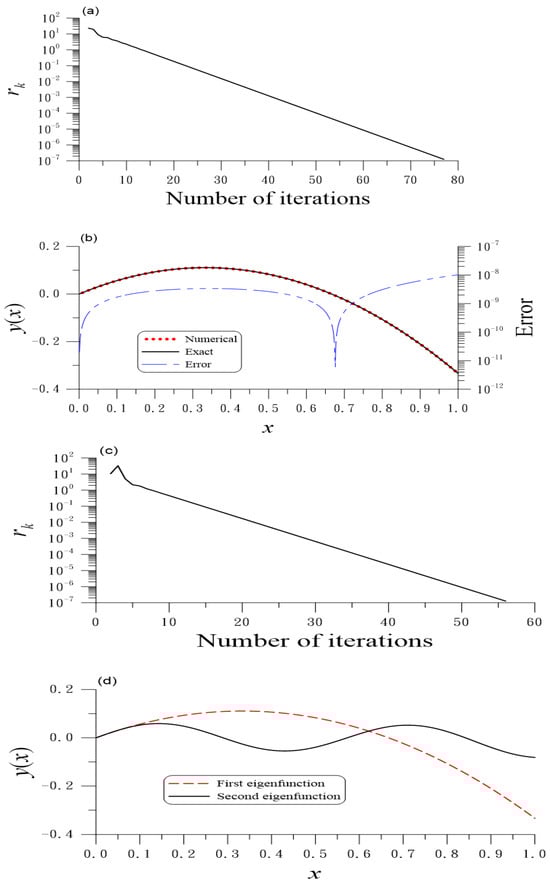
Figure 1. For example 6 of the first type nonlocal Sturm–Liouville problem, (a) the residuals and (b) numerical and exact solutions and error for the first eigenfunction; (c) the residuals and (d) numerical solution for the second eigenfunction.

If we raise the initial guess of ${\lambda }_0$ to ${\lambda }_0=100$, we obtain the second eigenvalue $\lambda =118.3439035468151$, which as shown in Figure 1c has 56 iterations and Figure 1d compares the first eigenfunction in Equation (76) to the second eigenfunction, of which $|y^{\prime }\left(1\right)-{\int }_0^{1}q\left(x\right)y\left(x\right)dx|=3.25 \times {10}^{-9}$. For the second eigenfunction, the analytic form is unknown.

5.5. Example 7

In Equations (53) and (54), we take

$$q\left(x\right)=\frac{581}{8}(8x^3-10x^2+3x)+48x-20,y\left(x\right)=x^3-\frac{5x^2}{4}+\frac{3x}{8}.$$

(77)

The exact eigenvalue is $\lambda =581/8=72.625$.

We can derive $p_1\left(x\right)=1-1.313285762827045x$, $p_2\left(x\right)=-0.08154943934760404x$. By taking $a_0=3/8$, $c_1=1$, $c_2=-1$, ${\alpha }_0=0$, ${\lambda }_0=72$, $N=1000$ and $ϵ={10}^{-2}$, Figure 2a shows six iterations for the convergence; upon comparing the computed $y\left(x\right)$ to the exact one, Figure 2b reveals ME = $3.07 \times {10}^{-4}$. The eigenvalue obtained has a relative error of $4.36 \times {10}^{-3}$. We obtain $|y^{\prime }\left(1\right)-{\int }_0^{1}q\left(x\right)y\left(x\right)dx|$ = $5.37 \times {10}^{-3}$.

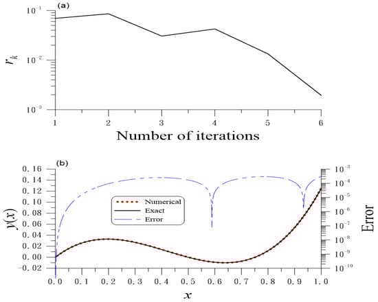
Figure 2. For example 7 of the first type nonlocal Sturm–Liouville problem, (a) the residuals and (b) numerical and exact solutions and errors.

6. Second Type Nonlocal Sturm–Liouville Problem

Instead of Equation (54), Albeverio et al. [35] consider

$$y\left(0\right)=0,y^{\prime }\left(1\right)+{\int }_0^{1}q\left(x\right)y\left(x\right)dx=0.$$

(78)

Equations (53) and (78) constitute the second type nonlocal Sturm–Liouville problem (NSLP). We can derive

$$p_1\left(x\right)=1-\frac{x{\int }_0^{1}q\left(x\right)dx}{1+{\int }_0^{1}xq\left(x\right)dx},p_2\left(x\right)=\frac{x}{1+{\int }_0^{1}xq\left(x\right)dx},$$

(79)

where we suppose that $1+{\int }_0^{1}xq\left(x\right)dx\ne 0$; $\lambda$ is computed by

$$\lambda =\frac{1}{{\int }_0^1{y}^2\left(x\right)dx}\left[{\int }_0^1{y}^{\prime }{\left(x\right)}^{2}dx+y\left(1\right){\int }_0^{1}q\left(x\right)y\left(x\right)dx-y\left(1\right)y^{\prime }\left(1\right)\right]=\frac{{\int }_0^1{y}^{\prime }{\left(x\right)}^{2}dx-2y\left(1\right)y^{\prime }\left(1\right)}{{\int }_0^1{y}^2\left(x\right)dx}.$$

(80)

For the second type NSLP we let

$$b_0:=u^{\prime }\left(1\right)+{\int }_0^{1}q\left(x\right)u\left(x\right)dx.$$

(81)

Liu and Qi [34] considered $q\left(x\right)=-90x^2+60x+6$, $y\left(x\right)=2x/3-x^2$; with the boundary conditions in Equation (78), a negative eigenvalue $\lambda =-30$ is obtained. For the positiveness of $\lambda$, the inequality ${\int }_0^1{y}^{\prime }{\left(x\right)}^{2}dx-2y\left(1\right)y^{\prime }\left(1\right)>0$ must hold. Through some operations for $y\left(x\right)=2x/3-x^2$, ${\int }_0^1{y}^{\prime }{\left(x\right)}^{2}dx-2y\left(1\right)y^{\prime }\left(1\right)=-4/9<0$ is obtained, which contradicts the above inequality. For the second type of NSLP, the eigenvalue may be negative.

In Section 6.3 and Section 6.4 two examples will be given to demonstrate that the solution $y\left(x\right)$ is not unique, even the conditions $y\left(0\right)=0$, $y^{\prime }\left(0\right)=a_0$ and $y^{\prime }\left(1\right)+{\int }_0^{1}q\left(x\right)y\left(x\right)dx=0$ are imposed. This is different from the local Sturm–Liouville problem; the uniqueness of $y\left(x\right)$ is guaranteed if $y\left(0\right)=0$ and $y^{\prime }\left(0\right)=a_0$ are imposed.

6.1. Iterative Algorithm

Let $\alpha =u_1\left(1\right)=u\left(1\right)$ and $\beta =u_2\left(1\right)=u^{\prime }\left(1\right)$ be unknown constants. The procedures for solving Equations (53) and (78) by the BSFM: (i) Give $q\left(x\right)$ and derive $p_1\left(x\right)$ and $p_2\left(x\right)$; give $c_1$, $c_2$, $a_0$, initial guesses of ${\lambda }_0$, ${\alpha }_0$, ${\beta }_0$, $ϵ$ and N. (ii) Calculate $b_0=[c_2-p_1^{\prime }\left(0\right)c_1-a_0]/p_2^{\prime }\left(0\right)$. (iii) For $k=0,1,2,\dots$, integrate Equation (73) by RK4 to offer

$${\alpha }_{k+1}=u_{1,k}\left(1\right),{\beta }_{k+1}=u_{2,k}\left(1\right),{\lambda }_{k+1}=\frac{u_{4,k}\left(1\right)-2[{\alpha }_{k+1}-G\left(1\right)][{\beta }_{k+1}-G^{\prime }\left(1\right)]}{u_{3,k}\left(1\right)};$$

(82)

terminate the iterations if

$$r_k=\sqrt{{({\alpha }_{k+1}-{\alpha }_k)}^2+{({\beta }_{k+1}-{\beta }_k)}^2+{({\lambda }_{k+1}-{\lambda }_k)}^2}<ϵ.$$

(83)

6.2. Infinite Solutions

We find that for the second NSLP, there may be many solutions with different ended values of the eigenfunctions. Hence, for the uniqueness of the eigenfunction of Equations (53) and (78), in addition to Equation (57), we can impose an extra condition:

$$y\left(1\right)=c_0,$$

(84)

where $c_0$ are some constants.

To resolve this problem by using the BSFM, we can set a suitable initial value of $c_1=u\left(0\right)$, such that the condition (84) can be satisfied. In Equation (69), we insert $x=1$ and use Equations (71) and (84) to obtain

$$c_0=u\left(1\right)-p_1\left(1\right)c_1-p_2\left(1\right)\frac{c_2-p_1^{\prime }\left(0\right)c_1-a_0}{p_2^{\prime }\left(0\right)},$$

(85)

where $u\left(0\right)=c_1$ and $u^{\prime }\left(0\right)=c_2$ were used. Then, we can compute $c_1$ by

$$c_1=\frac{p_2^{\prime }\left(0\right)c_0-p_2^{\prime }\left(0\right)u\left(1\right)+p_2\left(1\right)c_2-p_2\left(1\right)a_0}{p_2\left(1\right)p_1^{\prime }\left(0\right)-p_1\left(1\right)p_2^{\prime }\left(0\right)}.$$

(86)

For solving Equations (53) and (78) by the BSFM to find a particular solution with an ended value $y\left(1\right)=c_0$, we can modify the iterative algorithm in Section 6.1 to (i) Give $q\left(x\right)$ and derive $p_1\left(x\right)$ and $p_2\left(x\right)$; give $c_2$, $a_0$, ${\lambda }_0$, ${\alpha }_0$, ${\beta }_0$, $ϵ$ and N. (ii) For $k=0,1,2,\dots$, calculate

$$\begin{array}{c}{c}_1=\frac{p_2^{\prime }\left(0\right)c_0-p_2^{\prime }\left(0\right){\alpha }_k+p_2\left(1\right)c_2-p_2\left(1\right)a_0}{p_2\left(1\right)p_1^{\prime }\left(0\right)-p_1\left(1\right)p_2^{\prime }\left(0\right)},\hfill \end{array}$$

(87)

$$\begin{array}{c}{b}_0=\frac{c_2-p_1^{\prime }\left(0\right)c_1-a_0}{p_2^{\prime }\left(0\right)},\hfill \end{array}$$

(88)

integrate Equation (73) by RK4 and take

$${\alpha }_{k+1}=u_{1,k}\left(1\right),{\beta }_{k+1}=u_{2,k}\left(1\right),{\lambda }_{k+1}=\frac{u_{4,k}\left(1\right)-2[{\alpha }_{k+1}-G\left(1\right)][{\beta }_{k+1}-G^{\prime }\left(1\right)]}{u_{3,k}\left(1\right)}.$$

(89)

We terminate the iterations if

$$r_k=\sqrt{{({\alpha }_{k+1}-{\alpha }_k)}^2+{({\beta }_{k+1}-{\beta }_k)}^2+{({\lambda }_{k+1}-{\lambda }_k)}^2}<ϵ.$$

(90)

6.3. Example 8

In Equations (53) and (78), we take [35]

$$q\left(x\right)=2\pi sin\left(\pi x\right)+\pi sin\left(2\pi x\right).$$

(91)

The exact eigenvalue $\lambda ={\pi }^2$ is a multiple one, corresponding to multiple solutions $y\left(x\right)=sin\left(\pi x\right)$, $y\left(x\right)=xcos\left(\pi x\right)+sin\left(2\pi x\right)/\left(3\pi \right)$ and other.

We first consider $y\left(x\right)=sin\left(\pi x\right)$. We can derive $p_1\left(x\right)=1-8x/5$, $p_2\left(x\right)=2x/5$ and take $a_0=\pi$ for comparing the computed $y\left(x\right)$ to the exact one $y\left(x\right)=sin\left(\pi x\right)$. We take $c_1=1$, $c_2=2.19953$, ${\alpha }_0={\beta }_0=0$, ${\lambda }_0=9.5$, $N=500$ and $ϵ={10}^{-10}$. Figure 3a shows five iterations for the convergence; Figure 3b reveals high accuracy with ME = $4.34 \times {10}^{-6}$, AE$\left(\lambda \right)=2.56 \times {10}^{-10}$, and $|y^{\prime }\left(1\right)+{\int }_0^{1}q\left(x\right)y\left(x\right)dx|=1.17 \times {10}^{-9}$.

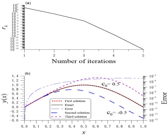
Figure 3. For example 8 of the second type nonlocal Sturm–Liouville problem, (a) the residuals and (b) numerical and exact solutions and error.

Using the iterative algorithm in Section 6.2, we take $c_0=0$ and $c_2=1$; through four iterations we obtain ME = $1.22 \times {10}^{-11}$, AE$\left(\lambda \right)=2.49 \times {10}^{-10}$ and $|y^{\prime }\left(1\right)+{\int }_0^{1}q\left(x\right)y\left(x\right)dx|=1.16 \times {10}^{-10}$. The accuracy of the eigenfunction is raised five orders, while the accuracy of the right boundary condition is raised one order.

When we take $c_0=-0.5$, AE$\left(\lambda \right)=6.56 \times {10}^{-10}$ and $|y^{\prime }\left(1\right)+{\int }_0^{1}q\left(x\right)y\left(x\right)dx|=1.42 \times {10}^{-10}$ are obtained through eleven iterations; as shown in Figure 3b remarked by $c_0=-0.5$, we obtain the second solution with an ended value $y\left(1\right)=-0.5$.

When we take $c_0=0.5$, AE$\left(\lambda \right)=3.09 \times {10}^{-11}$ and $|y^{\prime }\left(1\right)+{\int }_0^{1}q\left(x\right)y\left(x\right)dx|=1.44 \times {10}^{-11}$ are obtained through twenty iterations; as shown in Figure 3b remarked by $c_0=0.5$, we obtain the third solution with an ended value $y\left(1\right)=0.5$.

6.4. Example 9

Take $a_0=5/3$ for comparing the computed $y\left(x\right)$ to the exact one $y\left(x\right)=xcos\left(\pi x\right)+sin\left(2\pi x\right)/\left(3\pi \right)$. We take $c_1=c_2=1$, ${\alpha }_0={\beta }_0=0$, ${\lambda }_0=9$, $N=500$ and $ϵ={10}^{-10}$. Figure 4a shows 13 iterations for the convergence; Figure 4b reveals the high accuracy with ME = $1.27 \times {10}^{-8}$, AE$\left(\lambda \right)=6.61 \times {10}^{-10}$, and $|y^{\prime }\left(1\right)+{\int }_0^{1}q\left(x\right)y\left(x\right)dx|=3.26 \times {10}^{-11}$.

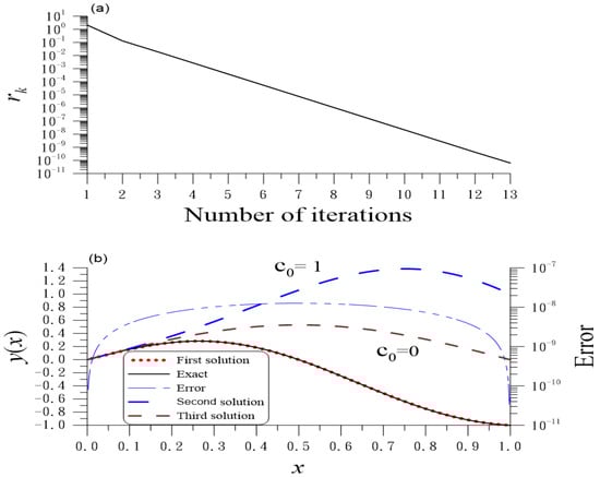
Figure 4. For example 9 of the second type nonlocal Sturm–Liouville problem, (a) the residuals and (b) numerical and exact solutions and error.

For this example, we also find other solutions, as shown in Figure 5 by a solid line, which is different from the first solution as shown by a thin dashed line in Figure 5. Although these two solutions have the same values of $y\left(0\right)=0$ and $y^{\prime }\left(0\right)=5/3$, the ended values are −1 and −0.2781268005, respectively. However, we do not have an analytic form of the second solution.

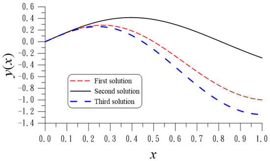
Figure 5. For example 9 comparing three solutions with different ended values.

Using the iterative algorithm in Section 6.2, when we take $c_0=1$, AE$\left(\lambda \right)=3.37 \times {10}^{-10}$ and $|y^{\prime }\left(1\right)+{\int }_0^{1}q\left(x\right)y\left(x\right)dx|=1.39 \times {10}^{-10}$ are obtained through 98 iterations; as shown in Figure 4b remarked by $c_0=1$, we obtain the second solution with an ended value $y\left(1\right)=1$.

When we take $c_0=0$, AE$\left(\lambda \right)=2.49 \times {10}^{-10}$ and $|y^{\prime }\left(1\right)+{\int }_0^{1}q\left(x\right)y\left(x\right)dx|=6.14 \times {10}^{-11}$ are obtained through four iterations; as shown in Figure 4b remarked by $c_0=0$, we obtain the third solution with an ended value $y\left(1\right)=0.5$.

Remark 1. 

There are two unconventional phenomena that happened for the second type of the nonlocal Sturm–Liouville problem. First, the eigenvalue may be negative depending on the end value of $y\left(1\right)y^{\prime }\left(1\right)$. Second, although the conditions $y\left(0\right)=0$ and $y^{\prime }\left(0\right)=a_0$ are imposed, the eigenfunction corresponding to the same eigenvalue is not unique, due to $y\left(1\right)$ appeared in Equation (53).

7. Precise Eigenvalue for the Nonlocal Sturm–Liouville Problem

As shown in example 6 in Section 5.4, the number of iterations (NI) is 77, and in example 7 in Section 5.5, the relative error of eigenvalue is $4.36 \times {10}^{-3}$. Basically, the slow convergence and low accuracy originate from considering one target equation in Equation (54). When Equation (61) is also deemed another target equation, we can improve the accuracy and reduce the number of iterations. Because we need to treat two nonlinear equations, the derivative-free iterative algorithm in Section 3.2 is not applicable.

To improve NI and accuracy, we note the derivative-free iterative algorithm in Section 3.2 by taking $b=0$ as a one-dimensional fixed-quasi-Newton method, and extend it to a two-dimensional fixed-quasi-Newton method (FQNM). It is known that the two-dimensional Newton method (including the quasi-one) is quadratically convergent. If we can enhance the convergence criterion $ϵ$ to a small value, we can achieve a highly accurate eigenvalue within a reasonable value of NI because both Equations (54) and (61) are accurately satisfied.

7.1. A Fixed-Quasi-Newton Method

For the first type nonlocal Sturm–Liouville problem in Section 5, it follows from Equations (54) and (61) and two nonlinear algebraic equations:

$$\begin{array}{c}{f}_1(A,B):=y^{\prime }\left(1\right)-{\int }_0^{1}q\left(x\right)y\left(x\right)dx=0,\hfill \end{array}$$

(92)

$$\begin{array}{c}{f}_2(A,B):=B{\int }_0^1{y}^2\left(x\right)dx-{\int }_0^1{y}^{\prime }{\left(x\right)}^{2}dx=0,\hfill \end{array}$$

(93)

where $A:=y\left(1\right)$ and $B:=\lambda$. Notice that $y\left(1\right)=A$ is appeared in the governing Equation (53), which makes $y\left(x\right)$ an implicit function of A; hence, $f_1$ and $f_2$ are also implicit functions of A.

As an extension of the one-dimensional FQNM in Section 3 with $b=0$, we now consider the approximation of a $2\times 2$ Jacobian matrix at the root $(A^{*},B^{*})$ of $f_1(A,B)=f_2(A,B)=0$ by finite differences, which is termed a fixed-quasi-Newton method (FQNM) of two-dimensions. Choose a rectangle with the vertexes $(A_0^{*},B_0^{*})$, $(A_2^{*},B_0^{*})$, $(A_2^{*},B_2^{*})$ and $(A_0^{*},B_2^{*})$ around the center point $[(A_0^{*}+A_2^{*})/2,(B_0^{*}+B_2^{*})/2]$ to carry out the approximation of the Jacobian matrix by a constant matrix $\left\{a_{ij}\right\}$.

The iterative algorithm obtained from the two-dimensional FQNM for solving $y\left(x\right)$ in Equations (53) and (54) is summarized as follows. (i) Give $A_0^{*}$, $A_2^{*}$, $B_0^{*}$, $B_2^{*}$, $ϵ$, and $\mathsf{\Delta }x=1/N$. (ii) Compute

$$\begin{array}{c}{A}_1^{*}=\frac{A_0^{*}+A_2^{*}}{2},B_1^{*}=\frac{B_0^{*}+B_2^{*}}{2},\hfill \\ a_{11}=\frac{f_1(A_2^{*},B_1^{*})-f_1(A_0^{*},B_1^{*})}{A_2^{*}-A_0^{*}},a_{12}=\frac{f_1(A_1^{*},B_2^{*})-f_1(A_1^{*},B_0^{*})}{B_2^{*}-B_0^{*}},\hfill \\ a_{21}=\frac{f_2(A_2^{*},B_1^{*})-f_2(A_0^{*},B_1^{*})}{A_2^{*}-A_0^{*}},a_{22}=\frac{f_2(A_1^{*},B_2^{*})-f_2(A_1^{*},B_0^{*})}{B_2^{*}-B_0^{*}},\hfill \\ C_{11}=\frac{a_{22}}{a_{11}{a}_{22}-a_{21}{a}_{12}},C_{12}=\frac{-a_{12}}{a_{11}{a}_{22}-a_{21}{a}_{12}},\hfill \\ C_{21}=\frac{-a_{21}}{a_{11}{a}_{22}-a_{21}{a}_{12}},C_{22}=\frac{a_{11}}{a_{11}{a}_{22}-a_{21}{a}_{12}}.\hfill \end{array}$$

(94)

(iii) Let $A_0=A_0^{*}$ and $B_0=B_0^{*}$ and for k = 0, 1, …, iterate

$$\begin{array}{c}{A}_{k+1}=A_k-C_{11}{f}_1(A_k,B_k)-C_{12}{f}_2(A_k,B_k),B_{k+1}=B_k-C_{21}{f}_1(A_k,B_k)-C_{22}{f}_2(A_k,B_k),\hfill \\ \mathrm{until}{r}_k:=\sqrt{f_1^2(A_k,B_k)+f_2^2(A_k,B_k)}<ϵ.\hfill \end{array}$$

(95)

Let $y_{1,k}\left(x\right)=y_{\left(k\right)}\left(x\right)$ and $y_{2,k}\left(x\right)=y_{\left(k\right)}^{\prime }\left(x\right)$. In each iteration, the RK4 is used to integrate

$$\begin{array}{c}{y}_{1,k}^{\prime }\left(x\right)=y_{2,k}\left(x\right),y_{1,k}\left(0\right)=0,\hfill \\ y_{2,k}^{\prime }\left(x\right)=q\left(x\right)A_k-B_k{y}_{1,k}\left(x\right),y_{2,k}\left(0\right)=a_0,\hfill \\ y_{3,k}^{\prime }\left(x\right)=y_{1,k}^2\left(x\right),y_{3,k}\left(0\right)=0,\hfill \\ y_{4,k}^{\prime }\left(x\right)=y_{2,k}^2\left(x\right),y_{4,k}\left(0\right)=0,\hfill \\ y_{5,k}^{\prime }\left(x\right)=q\left(x\right)y_{1,k}\left(x\right),y_{5,k}\left(0\right)=0,\hfill \end{array}$$

(96)

and calculate $f_1(A,B)=y_{2,k}\left(1\right)-y_{5,k}\left(1\right)$ and $f_2(A,B)=B{y}_{3,k}\left(1\right)-y_{4,k}\left(1\right)$.

7.2. Example 6 Again

We take $N=500$ and $ϵ={10}^{-15}$. Figure 6a shows 13 iterations, which converge faster than 77 iterations in Section 5.4. Figure 6b reveals a high accuracy with ME = $9.92 \times {10}^{-9}$ AE$\left(\lambda \right)=2.69 \times {10}^{-9}$, and $|y^{\prime }\left(1\right)-{\int }_0^{1}q\left(x\right)y\left(x\right)dx|=6.66 \times {10}^{-16}$.

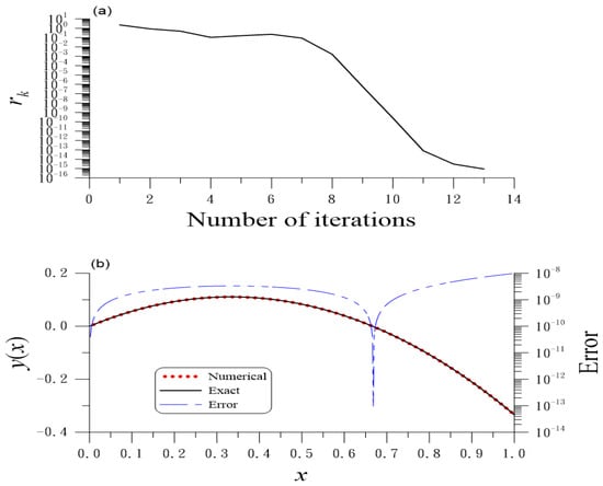
Figure 6. For example 6 solved by the FQNM, the improvements of (a) the residuals and (b) numerical and exact solutions and error.

7.3. Example 7 Again

We take $N=2000$ and $ϵ={10}^{-15}$. Figure 7a shows eight iterations for convergence. Upon comparison to Section 5.5 with six iterations under $ϵ={10}^{-2}$, the FQNM converges faster even with a stringent convergence criterion $ϵ={10}^{-15}$. Figure 7b reveals ME = $4.02 \times {10}^{-13}$. The eigenvalue obtained has a relative error of $3.14 \times {10}^{-12}$. The AE for $y^{\prime }\left(1\right)-{\int }_0^{1}q\left(x\right)y\left(x\right)dx$ is $7.77 \times {10}^{-16}$. The accuracy in every aspect is significantly improved by comparing to ME = $3.07 \times {10}^{-4}$, relative error = $4.36 \times {10}^{-3}$ and $|y^{\prime }\left(1\right)-{\int }_0^{1}q\left(x\right)y\left(x\right)dx|$ = $5.37 \times {10}^{-3}$ obtained in Section 5.5.

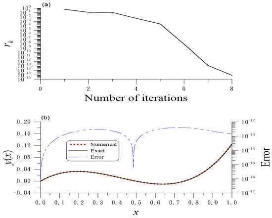
Figure 7. For example 7 solved by the FQNM, the improvements of (a) the residuals and (b) numerical and exact solutions and error.

7.4. Examples 8 and 9 Again

For the second type nonlocal Sturm–Liouville problem in Section 6, we apply the two-dimensional FQNM to solve

$$\begin{array}{c}{f}_1(A,B)=u_2\left(1\right)-G\left(1\right)+u_5\left(1\right)=0,\hfill \end{array}$$

(97)

$$\begin{array}{c}{f}_2(A,B)=B{u}_3\left(1\right)-u_4\left(1\right)+2[A-G\left(1\right)][u_2\left(1\right)-G^{\prime }\left(1\right)]=0,\hfill \end{array}$$

(98)

where $A=u\left(1\right)$ and $B=\lambda$. In each computation of $f_1(A,B)$ and $f_2(A,B)$, we need to integrate

$$\begin{array}{c}{u}_{1,k}^{\prime }\left(x\right)=u_{2,k}\left(x\right),u_{1,k}\left(0\right)=c_1,\hfill \\ u_{2,k}^{\prime }\left(x\right)=q\left(x\right)[A_k-G\left(1\right)]-B_k[u_{1,k}\left(x\right)-p_1\left(x\right)c_1-b_0{p}_2\left(x\right)],u_{2,k}\left(0\right)=c_2,\hfill \\ u_{3,k}^{\prime }\left(x\right)={[u_{1,k}\left(x\right)-p_1\left(x\right)c_1-b_0{p}_2\left(x\right)]}^2,u_{3,k}\left(0\right)=0,\hfill \\ u_{4,k}^{\prime }\left(x\right)={[u_{2,k}\left(x\right)-p_1^{\prime }\left(x\right)c_1-b_0{p}_2^{\prime }\left(x\right)]}^2,u_{4,k}\left(0\right)=0,\hfill \\ u_{5,k}^{\prime }\left(x\right)=q\left(x\right)[u_{1,k}\left(x\right)-G\left(x\right)],u_{5,k}\left(0\right)=0.\hfill \end{array}$$

(99)

For example 9 solved by the BSFM and two-dimensional FQNM, we take $N=1000$, $ϵ={10}^{-12}$, $c_1=c_2=1$. Through 14 iterations we obtain AE$\left(\lambda \right)=3.44 \times {10}^{-12}$, and $|y^{\prime }\left(1\right)+{\int }_0^{1}q\left(x\right)y\left(x\right)dx|=1.6 \times {10}^{-11}$. As shown in Figure 5 by a thick dashed line, we obtain the third solution with an ended value $y\left(1\right)=-1.25$.

For example 8 solved by the BSFM and two-dimensional FQNM, we take $N=1000$, $ϵ={10}^{-12}$, $c_1=1$, $c_2=1.3$. Through eleven iterations we obtain AE$\left(\lambda \right)=5.11 \times {10}^{-12}$, and $|y^{\prime }\left(1\right)+{\int }_0^{1}q\left(x\right)y\left(x\right)dx|=3.11 \times {10}^{-11}$. As shown in Figure 8, we obtain the second solution with an ended value $y\left(1\right)=-2.35619$. The solution of this problem is not unique even $y\left(0\right)=0$, $y^{\prime }\left(0\right)=\pi$ and $y^{\prime }\left(1\right)+{\int }_0^{1}q\left(x\right)y\left(x\right)dx=0$ are imposed.

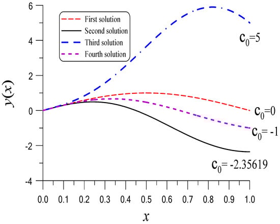
Figure 8. For example 8 comparing four solutions with different ended values. The first solution is obtained by the BSFM, while other solutions are obtained by the BSFM and FQNM.

We find that for the second type of NSLP in Section 6 there are many solutions with different ended values. To resolve this problem by using the BSFM, two-dimensional FQNM and the iterative method in Section 6.2, we take $c_0=5$ and $c_2=-1000$; AE$\left(\lambda \right)=8.99 \times {10}^{-12}$ and $|y^{\prime }\left(1\right)+{\int }_0^{1}q\left(x\right)y\left(x\right)dx|=5.87 \times {10}^{-11}$ are obtained. As shown in Figure 8 remarked by $c_0=5$, we obtain the third solution with an ended value $y\left(1\right)=5$. When we take $c_0=-1$ and $c_2=-1000$, AE$\left(\lambda \right)=3.37 \times {10}^{-11}$ and $|y^{\prime }\left(1\right)+{\int }_0^{1}q\left(x\right)y\left(x\right)dx|=2.12 \times {10}^{-11}$ are obtained. As shown in Figure 8 remarked by $c_0=-1$, we obtain the fourth solution with an ended value $y\left(1\right)=-1$. For example 9, we can also observe this phenomenon with many solutions corresponding to different ended values of the eigenfunctions.

8. Conclusions

Because two unknowns with a missing left-end value of the eigenfunction and eigenvalue are involved, the original generalized Sturm–Liouville problem is more difficult to solve than the presented formulation in the paper. We transformed the GSLP to a definite initial value problem. For the uniqueness of the eigenfunction, by giving a normalization condition we reduced two unknowns to an unknown for the eigenvalue, which is then solved from a target equation in terms of the right boundary condition. The proposed method converged very fast and example tests revealed the high precision of the eigenvalues obtained. We have resolved two types of NSLPs with integral boundary conditions specified on the right end. The appearance of nonlocal potential in the ODE led to some interesting phenomena, which are totally different from the SLP. The methods based on the boundary shape function methods and fixed-quasi-Newton methods were developed, which can accurately determine the eigenvalues and compute the eigenfunctions. For the first type of NSLP, an extra slope condition of the solution on the left end guarantees the uniqueness of the solution and the positiveness of the eigenvalue. For the second type of NSLP, two extra conditions of the slope of the solution on the left end and the specification of the ended value on the right end guarantees the uniqueness of the solution. For the second type of NSLP, the eigenvalue may be negative, and many different solutions happened for different end values. Four numerical testing examples demonstrated that the proposed iterative algorithm could achieve high precision eigenvalues. There are two factors to cause the high accuracy of eigenvalue and eigenfunction: the integration of the resulting ODEs by the fourth-order Runge–Kutta method and the boundary conditions being strictly satisfied.

The novelties involved in the paper were as follows:

• Mathematically transforming the generalized Sturm–Liouville problem to an initial value problem of a second-order ODE and an implicit nonlinear equation.
• Obtaining a very precise eigenvalue of the generalized Sturm–Liouville problem by using LHL on the implicit nonlinear equation.
• Mathematically transforming nonlocal Sturm–Liouville problems to the initial value problems and an implicit nonlinear equation.
• For nonlocal Sturm–Liouville problems the initial value problems and two implicit nonlinear equations were derived.
• The two-dimensional fixed-quasi-Newton method is used to solve two implicit nonlinear equations, quickly obtaining highly accurate eigenvalues.

References

- Aliyev, Y.N.; Kerimov, N. The basis property of Sturm–Liouville problems with boundary conditions depending quadratically on the eigenparameter. Arabian J. Sci. Eng. 2008, 33, 123–136. [Google Scholar]
- Binding, P.A.; Browne, P.J. Oscillation theory for indefinite Sturm–Liouville problems with eigenparameter-dependent boundary conditions. Proc. Royal Soc. Edinb. 1997, 127A, 1123–1136. [Google Scholar] [CrossRef]
- Chanane, B. Computation of the eigenvalues of Sturm–Liouville problems with parameter dependent boundary conditions using the regularized sampling method. Math. Comput. 2005, 74, 1793–1801. [Google Scholar] [CrossRef]
- Reutskiy, S.Y. A meshless method for nonlinear, singular and generalized Sturm–Liouville problems. Comput. Model. Eng. Sci. 2008, 34, 227–252. [Google Scholar]
- Reutskiy, S.Y. The method of external excitation for solving generalized Sturm–Liouville problems. J. Comput. Appl. Math. 2010, 233, 2374–2386. [Google Scholar] [CrossRef]
- Chanane, B. Sturm–Liouville problems with parameter dependent potential and boundary conditions. J. Comput. Appl. Math. 2008, 212, 282–290. [Google Scholar] [CrossRef][Green Version]
- Annaby, M.H.; Tharwat, M.M. On sampling theory and eigenvalue problems with an eigenparameter in the boundary conditions. SUT J. Math. 2006, 42, 157–175. [Google Scholar] [CrossRef]
- Chanane, B. Computing the spectrum of non-self-adjoint Sturm–Liouville problems with parameter-dependent boundary conditions. J. Comput. Appl. Math. 2007, 206, 229–237. [Google Scholar] [CrossRef]
- El-Gamel, M. Numerical comparison of sinc-collocation and Chebychev-collocation methods for determining the eigenvalues of Sturm–Liouville problems with parameter-dependent boundary conditions. SeMA J. 2014, 66, 29–42. [Google Scholar] [CrossRef]
- Aliyev, Y.N. Minimality properties of Sturm–Liouville problems with increasing affine boundary conditions. Operator Theo. Funct. Ana. Appl. 2021, 282, 33–49. [Google Scholar]
- Aydemir, K. Boundary value problems with eigenvalue depending boundary and transmission conditions. Boundary Value Prob. 2014, 2014, 131. [Google Scholar] [CrossRef][Green Version]
- Olgara, H.; Mukhtarova, O.S.; Aydemir, K. Some properties of eigenvalues and generalized eigenvectors of one boundary value problem. Filomat 2018, 32, 911–920. [Google Scholar] [CrossRef]
- Chu, J.; Meng, G.; Zhang, Z. Minimizations of positive periodic and Dirichlet eigenvalues for general indefinite Sturm–Liouville problems. Adv. Math. 2023, 432, 109272. [Google Scholar] [CrossRef]
- Zhang, H.; Chen, Y.; Ao, J.J. A generalized discontinuous Sturm–Liouville problem with boundary conditions rationally dependent on the eigenparameter. J. Differ. Equ. 2023, 352, 354–372. [Google Scholar] [CrossRef]
- Pandey, P.K.; Pandey, R.K.; Agrawal, O.P. Sturm’s theorems for generalized derivative and generalized Sturm–Liouville problem. Math. Commun. 2023, 28, 141–152. [Google Scholar]
- Farzana, H.; Bhowmik, S.K.; Alim, M.A. Bernstein collocation technique for a class of Sturm–Liouville problems. Heliyon 2024, 10, e28888. [Google Scholar] [CrossRef] [PubMed]
- Zhang, Z.; Wang, X. Sharp estimates of lowest positive Neumann eigenvalue for general indefinite Sturm–Liouville problems. J. Differ. Equ. 2024, 382, 302–320. [Google Scholar] [CrossRef]
- Belinskiy, B.P.; Smith, T.A. Optimal mass of structure with motion described by Sturm–Liouville operator: Design and predesign. Electron. J. Differ. Equ. 2024, 2024, 1–19. [Google Scholar] [CrossRef]
- Boucherif, A. Second order boundary value problems with integral boundary condition. Nonlinear Anal. 2009, 70, 364–371. [Google Scholar] [CrossRef]
- Dehghan, M. Numerical solution of a non-local boundary value problem with Neumann’s boundary conditions. Commun. Numer. Meth. Eng. 2003, 19, 1–12. [Google Scholar] [CrossRef]
- Chen, Z.; Jiang, W.; Du, H. A new reproducing kernel method for Duffing equations. Int. J. Comput. Math. 2021, 98, 2341–2354. [Google Scholar] [CrossRef]
- Ahmad, B.; Alsaedi, A.; Alghamdi, B.S. Analytic approximation of solutions of the forced Duffing equation with integral boundary conditions. Nonlinear Anal. Real World Appl. 2008, 9, 1727–1740. [Google Scholar] [CrossRef]
- Goodrich, C.S. On a nonlocal BVP with nonlinear boundary conditions. Results Math. 2013, 63, 1351–1364. [Google Scholar] [CrossRef]
- Webb, J.R.L.; Infante, G. Positive solutions of nonlocal boundary value problems involving integral conditions. Nonlinear Diff. Equ. Appl. 2008, 15, 45–67. [Google Scholar] [CrossRef]
- Liu, C.S.; Chang, J.R. Boundary shape functions methods for solving the nonlinear singularly perturbed problems with Robin boundary conditions. Int. J. Nonlinear Sci. Numer. Simul. 2020, 21, 797–806. [Google Scholar] [CrossRef]
- Liu, C.S. Accurate eigenvalues for the Sturm–Liouville problems, involving generalized and periodic ones. J. Math. Research 2022, 14, 1–19. [Google Scholar] [CrossRef]
- Peciulyte, S.; Stikoniene, O.; Stikonas, A. Sturm-Liouvelle problem for stationary differential operator with nonlocal integral boundary condition. Math. Model. Anal. 2005, 10, 377–392. [Google Scholar] [CrossRef]
- Stikonas, A. The Sturm-Liouvelle problem with a nonlocal boundary condition. Liet. Mat. Rink. 2007, 47, 410–428. [Google Scholar]
- Nizhnik, L.P. Inverse eigenvalue problems for nonlocal Sturm-Liouvelle operators. Meth. Func. Anal. Topol. 2009, 15, 41–47. [Google Scholar]
- Stikonas, A.; Stikoniene, O. Characteristic functions for Sturm–Liouville problems with nonlocal boundary conditions. Math. Model. Anal. 2009, 14, 229–246. [Google Scholar] [CrossRef]
- Kandemir, M.; Mukhtarov, O.S. Nonlocal Sturm–Liouville problems with integral terms in the boundary conditions. Elect. J. Diff. Equ. 2017, 2017, 1–12. [Google Scholar]
- Stikonas, A. A survey on stationary problems, Green’s functions and spectrum of Sturm–Liouville problem with nonlocal boundary conditions. Nonl. Anal. Contr. 2014, 19, 301–334. [Google Scholar] [CrossRef]
- Liu, C.S.; Hong, H.K.; Lee, T.L. A splitting method to solve a single nonlinear equation with derivative-free iterative schemes. Math. Comput. Simul. 2021, 190, 837–847. [Google Scholar] [CrossRef]
- Liu, Z.; Qi, J. The properties of eigenvalues and eigenfunctions for nonlocal Sturm–Liouville problems. Symmetry 2021, 13, 820. [Google Scholar] [CrossRef]
- Albeverio, S.; Hryniv, R.O.; Nizhnik, L.P. Inverse spectral problems for non-local Sturm–Liouville operators. Inv. Prob. 2007, 23, 523–535. [Google Scholar] [CrossRef]
Disclaimer/Publisher’s Note: The statements, opinions and data contained in all publications are solely those of the individual author(s) and contributor(s) and not of MDPI and/or the editor(s). MDPI and/or the editor(s) disclaim responsibility for any injury to people or property resulting from any ideas, methods, instructions or products referred to in the content. |
© 2024 by the authors. Licensee MDPI, Basel, Switzerland. This article is an open access article distributed under the terms and conditions of the Creative Commons Attribution (CC BY) license (https://creativecommons.org/licenses/by/4.0/).