HCEL: Hybrid Clustering Approach for Extending WBAN Lifetime

Abstract

Wireless body area networks (WBANs) have emerged as a promising solution for addressing challenges faced by elderly individuals, limited medical facilities, and various chronic medical conditions. WBANs consist of wearable sensing and computing devices interconnected through wireless communication channels, enabling the collection and transmission of vital physiological data. However, the energy constraints of the battery-powered sensor nodes in WBANs pose a significant challenge to ensuring long-term operational efficiency. Two-hop routing protocols have been suggested to extend the stability period and maximize the network’s lifetime. These protocols select appropriate parent nodes or forwarders with a maximum of two hops to relay data from sensor nodes to the sink. While numerous energy-efficient routing solutions have been proposed for WBANs, reliability has often been overlooked. Our paper introduces an energy-efficient routing protocol called a Hybrid Clustering Approach for Extending WBAN Lifetime (HCEL) to address these limitations. HCEL leverages a utility function to select parent nodes based on residual energy (RE), proximity to the sink node, and the received signal strength indicator (RSSI). The parent node selection process also incorporates an energy threshold value and a constrained number of serving nodes. The main goal is to extend the overall lifetime of all nodes within the network. Through extensive simulations, the study shows that HCEL outperforms both Stable Increased Throughput Multihop Protocol for Link Efficiency (SIMPLE) and Energy-Efficient Reliable Routing Scheme (ERRS) protocols in several key performance metrics. The specific findings of our article highlight the superior performance of HCEL in terms of increased network stability, extended network lifetime, reduced energy consumption, improved data throughput, minimized delays, and improved link reliability.

1. Introduction

Healthcare spending has shown a substantial global increase recently, particularly in the United Arab Emirates (UAE). In 2020, healthcare expenditure in the UAE increased by 5.67% [1] and is projected to grow by nearly one-third in the coming years [2]. Several factors contribute to this upward trajectory, including the aging population and the prevalence of lifestyle diseases, highlighting the increasing demand for accessible and effective healthcare services [1,2]. Consequently, there is a pressing need to explore innovative approaches that can meet the needs of patients, especially in remote areas or situations where physical hospital visits pose challenges. Finding cost-effective and convenient ways to deliver healthcare services is essential to ensure that individuals receive the care they require [3,4,5].

Technological advancements have played an essential role in addressing these challenges. A notable innovation is the integration of remote care providers or hospitals, which allow the delivery of healthcare services from a distance [5,6]. In this context, WBANs have emerged as a significant trend that offers promising opportunities for remote healthcare monitoring [5,6,7,8,9]. WBANs are considered a subset of wireless sensor networks (WSNs) and also represent the next generation of personal area networks (PANs) [5,10,11,12,13,14,15]. Additionally, WBANs may contain various types of physiological, kinematic, and ambient sensors. These sensors capture and measure different parameters related to the human body and the environment, providing valuable insights into an individual’s health status [7,16,17,18]. In WBANs, small sensor nodes (edge nodes) are strategically placed within a range of 1–2 m [12,13] from the central node, known as the sink node or coordinator node. The sink node has enhanced resource capabilities to handle data from all sensor nodes and transmit them to the cloud for remote analysis.

WBANs may have implanted or wearable sensors [11,12,13,15,19]. Implanted sensors are designed to be placed inside the human body, while wearable sensors are externally attached to the body, allowing for non-invasive monitoring of physiological and environmental data. The applications of WBANs span medical and non-medical domains [11,12,13,15,19]. In the medical field, WBANs facilitate real-time health monitoring, remote patient management, and early detection of medical emergencies. For instance, WBANs can monitor vital signs like heart rate, blood pressure, and body temperature, allowing health professionals to remotely assess a patient’s health status and provide timely interventions. In non-medical applications, WBANs contribute to various sectors such as monitoring circadian rhythms, supporting battlefield healthcare for military personnel, and enhancing interactive gaming experiences by capturing real-time physiological responses [10,15,16,18,20,21].

Implementing WBANs poses several challenges, with a primary concern of energy efficiency [11,12,13,15,19]. To address these challenges, various routing protocols have been proposed; however, most existing protocols designed for WSNs are not directly applicable to WBANs due to unique constraints in WBANs. WBANs operate with limitations on the number of sensor nodes and the distances between nodes placed on the human body. Consequently, for instance, finding multiple sensors capable of performing the same task, which is applicable in WSNs, becomes constrained in WBANs. In addition, the routing protocols in WBANs only transmit the packets with a maximum of two hops. One of the key requirements for WBANs is also efficient energy utilization, considering the limited power resources of sensor nodes. The existing limitations in WBANs underscore the need for designing new routing protocols tailored to these networks.

Among the different types of routing protocols, clustering-based protocols have shown promise for WBANs [3,4,5,6,22,23,24,25]. These protocols group edge nodes into clusters, with a designated parent node for each cluster responsible for data aggregation and transmission to the sink node for remote management and analysis. These clustering-based protocols optimize energy usage by selecting an intermediate node (a parent node) that shortens the distance between the sensor nodes and the sink node. However, the selection criteria for the parent (forwarder) node on a round-by-round basis are based on factors that may lead to an uneven distribution of traffic among sensor nodes, potentially minimizing the network lifespan. Hence, enhancing the selection criteria for parent nodes becomes crucial for improving the overall efficiency of energy utilization in WBANs.

To address the limitations in existing cluster-based routing protocols, this paper introduces a novel routing protocol, called the HCEL (Hybrid Clustering Approach for Extending WBAN Lifetime). The HCEL routing protocol combines the benefits of static clustering (i.e., fixed parent node until it depletes its energy) and dynamic clustering (i.e., flexible parent node selection) to optimize energy consumption and enhance network lifetime. The proposed HCEL routing protocol encompasses three key phases: network deployment and initialization, parent node selection, and data transmission. In the network deployment and initialization phase, the WBAN is established, and initial operations are performed to ensure the smooth functioning of the deployed nodes. Sensor nodes are strategically placed during this phase, and the network is initialized for subsequent operations. The parent node selection phase plays a key role in HCEL. It involves selecting parent nodes within the network that serve as intermediaries for data transmission from sensor nodes to the sink. The selection process is guided by an energy-efficient algorithm considering factors such as (1) node energy levels, (2) distance to the sink, and (3) the received signal strength indicator (RSSI). Moreover, the selected node must adhere to constraints, including the number of serving nodes ($\tau$) and the threshold value of the candidate parent nodes’ energy ($Th$). By carefully choosing parent nodes, the HCEL approach aims to achieve balanced energy consumption and prevent the nodes from prematurely depleting their energy resources.

Once the parent nodes are selected, the data transmission phase begins. Sensor nodes within the WBAN collect data from various physiological sensors and transmit them to the sink node. Critical data are transmitted directly (one hop) to the sink, while regular data are transmitted through the selected parent nodes (two hops) to the sink. The sink node acts as the central hub, receiving and processing the data for further analysis or storage. Throughout this phase, the sink node continuously monitors the energy levels of the sensor nodes. This monitoring mechanism helps to prevent node failures and prolong the overall lifetime of sensor nodes. The proposed HCEL approach offers several advantages over traditional WBAN systems as follows: (1) Combining static and dynamic clustering leverages clustering benefits, resulting in improved energy efficiency and network stability, and (2) the parent node selection process further enhances these benefits by ensuring load balancing among sensor nodes. As a result, the HCEL protocol extends the lifetime of sensor nodes, reducing energy consumption and enhancing the overall performance of the WBAN system.

The paper follows a well-structured organization to present the research findings. Section 2 provides an overview of related work conducted in the context of this article, giving readers a comprehensive understanding of existing research works. Section 3 introduces key preliminaries for comprehending the proposed scheme and the experiments conducted. In Section 4, the paper delves into the heart of the study by presenting the proposed routing protocol, HCEL, in detail. Moving forward, Section 5 presents the simulation results and analysis, shedding light on the performance of the proposed HCEL protocol. Finally, Section 6 closes the article by summarizing the research’s key findings, contributions, and implications.

2. Related Work

WBANs encounter many challenges due to the nature of the sensors and the environments in which they operate. One of the challenges in WBANs is the limited data rate, which ranges from a few kilobits per second (kbps) to several megabits per second (Mbps) [12,13]. This limitation poses a hurdle for transmitting sensor data to the sink node. Furthermore, the movement and dynamic nature of the human body [26,27] alter the radio frequency environment, resulting in interference and signal attenuation [11]. The security and privacy of the data transmitted in a WBAN can also be another challenge. Special precautions must be taken to maintain data privacy and integrity due to the sensitive nature of physiological data acquired in WBANs [28,29,30,31]. Some methods can be used to guarantee data confidentiality and integrity, such as access control systems or encryption algorithms. However, using these techniques incurs overhead for data transmission.

One of the most significant challenges in designing WBANs is the restricted energy source for wearable sensors. A constrained network lifetime is the result of these sensors often being battery-powered and difficult to recharge or replace. In other words, the energy constraints are mainly due to the limited battery capacity, the small size of the sensors, and the need for the sensors to be continuously operational [7,13]. Therefore, optimizing energy consumption is essential to extending the WBAN’s lifespan. The challenge of energy efficiency in WBANs has been addressed using several techniques. One technique is replenishing the sensors’ battery using energy harvesting techniques [16,17,18,32], such as solar or kinetic energy. This approach can increase the lifetime of the WBAN by reducing the need for battery replacement or recharging. Energy harvesting techniques, however, require appropriate hardware and are not ideal for all kinds of sensors. Additionally, sleep scheduling and duty cycling techniques can be used to conserve energy by turning off the sensors when not needed [12,33,34].

In conjunction with the previous techniques, one of the most common techniques is the development of energy-efficient routing protocols [19,35,36]. When designing WBANs, routing is paramount to ensuring effective and reliable data transmission [8,21]. A routing protocol determines the optimal path for data transmission from the sensors to the sink node to minimize the sensors’ energy consumption during data transmission. The lifetime and performance of the WBAN are increased by reducing the energy consumption of the sensors. Routing protocols in WBANs can be classified into several categories according to their functionality and mode of operation, including cross-layer, postural, QoS-aware, thermal-aware, and cluster-based [8,11,12,13,15,19,21].

In cross-layer routing protocols, the routing decision is made based on information gathered from different layers of the protocol stack, such as physical, MAC, and network layers, to optimize network performance [35,37]. In traditional networking, each layer operates independently, and information flows only vertically between adjacent layers. However, in cross-layer design, information can be exchanged horizontally between different layers, allowing for more efficient use of network resources and better performance. It is particularly beneficial for optimizing energy consumption and network lifetime [37,38]. By leveraging information from different protocol stack layers, cross-layer routing protocols can make more informed decisions about routing paths and power management. For example, using information from the MAC layer, such as the status of the medium access control protocol and the buffer status of the nodes, cross-layer routing protocols can make more efficient use of the available bandwidth and reduce collisions, leading to improved network performance. Despite the advantages mentioned earlier, some challenges of cross-layer design include the increased complexity of the protocol stack and conflicts between different layers due to the exchange of information. Examples of cross-layer routing protocols in WBANs include WASP (Wireless Autonomous Spanning Tree Protocol) [39], CICADA (Cascading Information of Controlling Access and Distributed Slot Assignment) [40], TICOSS (Time-Zone Coordinated Sleeping Scheme) [34], Biocomm (a communication protocol for biomedical sensor networks) [41], and AMR (Adaptive Multihop Tree-Based Routing) [42].

Postural routing protocols leverage the specific structure and posture of the human body, such as the relative positions and orientations of the sensors on the body, to improve the efficiency of data transmission [26,27,43,44]. It uses this information to make routing decisions that minimize the energy consumption of the sensor nodes and improve the reliability of the network. For example, postural routing protocols can improve the network’s overall reliability and energy efficiency by selecting routes that avoid interference caused by body movement or selecting nodes with stronger signals due to their position on the body. However, postural routing protocols may face some limitations, such as the need for accurate posture sensing and interference from body movement. Examples of a postural routing protocol in WBANs are Opportunistic (opportunistic routing based on posture prediction) [45], DVRPLC (Distance-Vector Routing Protocol with Postural Link Costs) [46], and OBSFR (On-body Store and Flood Routing Protocol) [14].

Quality of Service (QoS) is important in WBANs since some applications require real-time data transmission and reliable communication. QoS-aware routing protocols consider the QoS requirements of different applications, such as delay, reliability, and energy efficiency, and prioritize them for routing decisions accordingly [47]. For example, for applications that require low latency and high reliability, QoS-aware routing protocols can prioritize routes with low delay and high link quality. Conversely, for applications that are more tolerant to delay but require low energy consumption, QoS-aware routing protocols can prioritize routes with low energy consumption and choose one irrespective of how long it takes. QoS-aware routing protocols can improve overall performance by providing differentiated services to different types of traffic and by meeting the QoS requirements of each application. However, it may increase the complexity of the routing protocol and the QoS conflicts between different applications. Examples of QoS-aware routing protocols in WBANs include DMQoS (Data-Centric Multi-Objective QoS-based routing protocol) [48], QPRD (delay-sensitive data QoS-aware routing protocol) [49], EPR (Energy-Aware Peering routing protocol) [50], TMQoS (Thermal-Aware Multi-Constrained Intrabody QoS routing protocol) [51], and DARE (Distance-Aware Relaying Energy-Efficient System) [52].

The thermal-aware routing protocol uses the temperature information from sensor nodes to make routing decisions. It aims to balance the trade-off between energy and temperature control to ensure the reliable operation of the sensors. Temperature information is used to estimate energy consumption and predict the lifetime of sensor nodes [53,54]. Thermal-aware routing protocols can reduce energy consumption and prevent sensor nodes from overheating by avoiding routes that pass through nodes with high temperatures. Furthermore, these protocols can increase the lifetime of the sensor nodes by distributing the traffic load across the network. However, there are some challenges, such as the need for accurate temperature sensing and the complexity of the routing algorithm. Examples of a temperature-based routing protocol in WBANs are $M^2{E}^2$ (Multimode Energy-Efficient Multi-Hop protocol) [55], RE-ATTEMPT (Reliability-Enhanced Adaptive Threshold-Based Thermal-Unaware Energy-Efficient Multi-Hop protocol) [56], MATTEMPT (Mobility-Supporting Adaptive Threshold-Based Thermal-Aware Energy-Efficient Multi-Hop protocol) [57], TMQoS (Thermal-Aware Multi-Constrained Intrabody QoS routing protocol) [51], ETPA (Energy-Efficient, Thermal, and Power-Aware routing protocol) [58], ALTR (Adaptive Less Temperature Rise) [59], LTRT (Least Total Route Temperature) [60], and TARA (Thermal-Aware Routing Algorithm) [61].

The cluster-based routing protocol reduces the amount of data transmission and the distance between the sensors and the sink node, leading to reduced energy consumption and improved network lifetime. However, the choice of cluster heads may affect the network’s overall performance. Examples of clustered routing protocols in WBANs include SIMPLE (Stable Increased Throughput Multihop Protocol for Link Efficiency) [24], iM-SIMPLE (Improved-SIMPLE) [23], FEEL (Forwarding Energy-Efficient Data with Load Balancing) [4], ERRS (Energy-Efficient Reliable Routing Scheme) [25], LAEEBA (Linked-Aware Energy-Efficient routing protocol) [22], CO-LAEEBA (Cooperative-LAEEBA) [6], and DSCB (Dual Sink Approach Using Clustering in Body Area Network) [5]. On the basis of the above discussions, the cluster-based routing protocol is the most suitable for WBAN applications. This paper aims to improve the energy efficiency of the network and extend the lifetime of the network by clustering the sensor nodes into groups [35]. Each cluster has a cluster head, which serves as an intermediary node and is responsible for collecting data from the sensor nodes and forwarding it to a sink node.

Table 1 summarizes the different cluster-based routing protocols employed in WBANs and compares them with our proposed routing protocol (HCEL). The table highlights essential information, such as the criteria used for parent node selection, advantages, limitations, clustering approach, and the number of sink nodes.

Table 1. Summary of cluster-based routing protocols in WBANs.

Protocol	Parent Selection Criteria	Advantages	Limitations	Type of Clustering	Number of Sink Nodes
SIMPLE [24]	Minimum $CF$ 2 $CF=\frac{{dist}^1}{{RE}^5}$	Maximize throughput, Balance residual energy across sensors.	Unequal distribution of traffic load among sensors, Low performance of the protocol in crucial data due to frequent data transfer, Large overhead in communication cost, Assume stationary nodes.	Static	Single
iM-SIMPLE [23]	Same as SIMPLE	Handle mobility, Maximize throughput.	Picking closer nodes frequently, Ignoring link quality and path loss, Large number of dropped packets.	Static	Single
FEEL [4]	Maximum $RE$ 5	Balance energy consumption of the network.	Ignoring path failure, Less intention to retransmit data packets, Assuming stationary nodes.	Static	Single
ERRS [25]	Minimum $WF$ 3 $WF=\frac{{dist }^1}{{RE}^5}$	Load balance by selecting new parent node after several data transmission rounds.	Ignoring scalability, Assuming stationary nodes.	Static + Dynamic	Single
LAEEBA [22]	Minimum $CF$ 2 $CF=\frac{\sqrt{{dist}^1}}{{RE}^5}$	Reliable, Minimum path loss, High network lifetime.	More overhead of data packets during data communication, Assuming stationary nodes.	Static	Single
CO-LAEEBA [6]	Maximum $RE$ 5 for parent node	Consider data priority, Maximum throughput, High network lifetime.	Limited number of parent nodes used, Require many links between sensors and sink for packet delivery, Assuming stationary nodes.	Static + Dynamic	Single
BEC [3]	Minimum $CF$ 2 $CF=\frac{1}{{RE}^5}$	Works well in terms of network lifetime, Uniform load distribution.	Parent node consumes more energy due to the demanding task of forwarding, Assuming stationary nodes.	Static	Single
DSCB [5]	Minimum $CF$ 2 $CF=\frac{{dist}^1}{{RE}^5 \times {TP}^4}$	Balance network load due to the double sinks used, Improve negative consequences of the shadow effect causes.	Disregarding energy efficiency with node cooperation and energy harvesting for efficient routing, Assuming stationary nodes.	Static	Double
HCEL	Maximum $CF$ 2 $CF=\frac{{dist }^1 \times RSSI}{{RE }^5}$	Equal distribution of traffic load by combining static and dynamic clustering, Extend sensor nodes’ lifetimes, Improve overall network performance and reliability.	Assuming stationary nodes.	Static + Dynamic	Single

¹ dist refers to the distance between the sensor node and the sink node, ² CF represents a cost function, ³ WF is a weight factor, ⁴ TP is a transmission power, and ⁵ RE represents residual energy.

Most cluster-based routing protocols are built on a static clustering strategy. This static approach keeps the parent node (e.g., nodes close to the sink) unchanged until it depletes its energy (i.e., dies), resulting in decreased network efficiency. In contrast, dynamic clustering involves a flexible selection and adjustment of the parent node based on the current state of the network. The choice of the parent node is dynamically modified to adapt to changes in node energy levels, connectivity, or other network conditions. Although dynamic clustering improves network performance, it often incurs additional overhead and complexity, as the cluster structure needs to be frequently updated and modified.

To overcome the limitations of static and dynamic clustering, we propose an energy-efficient routing strategy called HCEL. In our routing protocol, we prioritize the selection of parent nodes based on factors like distance, residual energy, and RSSI. Unlike static clustering approaches where the same node is chosen until its energy is depleted, our protocol selects a different parent node after several data transmission rounds. Our routing protocol considers other parameters, such as the number of the nodes that the parent node can serve ($\tau$) and the threshold energy for all parent candidates ($Th$). By incorporating these factors, the selection of the parent node is adjusted based on the current state of the network, effectively combining the benefits of both static and dynamic clustering. This adjustment ensures a balanced distribution of the load across all nodes, preventing any individual node from being overwhelmed with data forwarding tasks. By combining both the static and dynamic clustering, we enhance the network lifetime, stability period, energy consumption, and overall performance.

3. Preliminaries

This section introduces our system, assumptions, energy, and path loss models. Moreover, it presents the various performance measures used in our simulation analysis.

3.1. System Model and Assumptions

Our model is based on graph theory [62], represented as an undirected graph $G=(V,E)$. The graph consists of a set of vertices V representing the network’s nodes $v_i\in V$ and a set of edges E that connect nodes together. Any edge $e_{ij}\in E$ is formed between any two nodes, $v_i$ and $v_j$, when the two nodes are in the transmission range of each other.

This paper relies on assumptions to establish, model, and analyze our network. The first assumption is that all network nodes are stationary, meaning their positions and network topology remain fixed throughout the analysis. Except for the sink node, all nodes are assumed to have the same capabilities, equal importance, and initial energy levels. Data transmission is categorized into one-hop for critical data and two-hop for normal data. Moreover, the nodes, excluding the sink node, are equipped with routing functionality but are constrained regarding resources, encompassing energy, and processing capabilities.

3.2. Energy Model

We use the first-order radio energy model as presented in Ref. [63]. This model provides mathematical equations to characterize the energy consumption during data transmission and reception processes in WBANs. The energy consumption of the transmitter and receiver is given by Equations (1) and (2), respectively:

$$E_{Tx}(k,d)=E_{Tx-elec}\times k+E_{amp}\times \eta \times k\times d^{\eta }$$

(1)

$$E_{Rx}\left(k\right)=E_{Rx-elec}\times k.$$

(2)

In Equation (1), $E_{Tx}(k,d)$ represents the total energy consumption (in joules) required to transmit k bits between two nodes (e.g., $v_i$ and $v_j$) with a separation distance of d. Here, $E_{Tx-elec}$ is the energy (in joule/bit) needed in the transmitter’s circuits, while $E_{amp}$ is the energy (in joule/bit/m^η) consumed by the amplifier circuit in the transmitter. $\eta$ is the path loss coefficient. Moving on to Equation (2), $E_{Rx}\left(k\right)$ is the amount of energy consumed (in joules) by the receiver. Within this equation, $E_{Rx-elec}$ accounts for the energy (in joule/bit) utilized in the receiver’s circuits. The values for the path loss coefficient $\eta$ in Equation (1) are provided as follows [4]:

$$\eta =\left\{\begin{array}{cc}2\hfill & \mathrm{free}\mathrm{space};\hfill \\ 3–4\hfill & \mathrm{line}\mathrm{of}\mathrm{sight}\left(\mathrm{LOS}\right);\hfill \\ 5–7.4\hfill & \mathrm{non-line}\mathrm{of}\mathrm{sight}\left(\mathrm{NLOS}\right).\hfill \end{array}\right.$$

In our work, we account for the impact of signal degradation caused by various factors in a WBAN. These factors include obstacles like the body, walls, furniture, and indoor objects that can affect the line-of-sight transmission between sensor nodes on different body parts. To incorporate this attenuation into our analysis, we utilize an attenuation factor of $\eta =3.38$ [23]. This factor quantifies the influence of these obstacles on the strength of the transmitted signal.

The energy parameters used in our analysis, such as $E_{tx-elec}$, $E_{Rx-elec}$, and $E_{amp}$, are hardware-dependent and specific to the system under consideration. Although several transceivers are commonly used in WBANs, we specifically employ the Chipcon CC2420 transceiver in our research. Detailed energy parameters for this transceiver are provided in Table 2 [4,23,24,57]. By considering the impact of signal attenuation due to obstacles and utilizing the energy parameters specific to the Chipcon CC2420 transceiver, we ensure that our analysis accurately reflects the real-world performance of the WBAN system under investigation.

Table 2. Energy parameters for the Chipcon CC2420 transceiver.

Parameters	Value	Units
$E_{tx-elec}$	96.9	nJ/bit
$E_{Rx-elec}$	172.8	nJ/bit
$E_{amp}$	$2.71\times {10}^{-7}$	J/bit/mη

To calculate the energy consumption in our proposed routing strategy, we consider the residual energy (RE) of each node in the network. This is calculated by subtracting the consumed energy from the initial energy. The energy consumed during data transmission by a sensor node is represented by Equation (1). However, for the parent node, the energy consumption includes the terms of Equation (1) and the energy consumed in the reception process, as expressed by Equation (2). This distinction arises because the parent node not only receives data from the sensor node but also forwards it to the sink.

3.3. Path Loss

Path loss in WBAN refers to the attenuation or reduction in signal power as it travels through the human body or the surrounding environment. It can be captured by different models based on the application and the environment in which sensors are placed [64]. In this work, we use a log-distance path loss model, which considers the effect of obstacles and objects as well as various environmental factors such as attenuation, reflection, diffraction, and scattering. The model is proportional to the logarithm of the distance between the transmitter (e.g., sensor node) and the receiver (e.g., parent or sink node). In Equation (3), the power loss $PL\left(d\right)$ is modeled as a linear function of the distance (d) between the transmitter and receiver [65]:

$$PL\left(d\right)=P{L}_0-10\eta {log}_{10}\frac{d}{d_0}+X_{\sigma },$$

(3)

where $d_0<d$, $P{L}_0$ is the power loss at the reference distance $d_0$ (defined in Equation (4)), and $X_{\sigma }$ is the Gaussian random variable with zero mean and standard deviation $\sigma$.

In practice, it is difficult to predict the strength of the signal between the transmitter and the receiver [24]. Thus, the random variable ($X_{\sigma }$) is used to model the effect of shadowing and multipath fading. In addition, $P{L}_0$ is used as a reference for comparing the path loss at other distances in the case where there is no shadowing or multipath fading:

$$P{L}_0=10{log}_{10}{\left(\frac{4\ast \pi \ast d}{\lambda }\right)}^2$$

(4)

where $\lambda$ is the electromagnetic wavelength, $\lambda =\frac{c}{f}$, c is the speed of light ($3\ast {10}^8$ m/s), and f is the frequency.

3.4. Performance Metrics

In this section, we present different performance metrics that will be used in our experiment analysis (see Section 5) to assess our proposed routing protocol.

3.4.1. Network Lifetime and Stability Period

The network lifetime and stability period are closely related metrics in WBANs, both vital for ensuring the overall performance and reliability of the network. The network lifetime refers to the duration for which the network can operate before the energy of the nodes is completely depleted. At the same time, the stability period represents the time from network initiation until the first node becomes non-operational due to energy exhaustion. Maximizing the network lifetime is a fundamental objective in WBAN design, and it directly impacts the stability period. Prolonging the stability period, in turn, contributes to extending the overall lifetime of the network, allowing continuous monitoring and data transmission, which is particularly necessary in applications such as healthcare systems.

Several factors influence both the network lifetime and the stability period in WBANs. One significant factor is the energy consumption of the sensor nodes, which occurs during data transmission, reception, processing, and sensing activities. Efficient routing protocols play a vital role in balancing the energy consumption among nodes and optimizing the utilization of energy resources. Uneven energy consumption can lead to premature depletion of certain nodes, creating energy holes and reducing the overall network lifetime [25,47]. To address this, load balancing techniques can distribute the workload evenly across the nodes, preventing energy exhaustion in specific nodes, particularly those near the sink. Furthermore, selecting appropriate parent nodes for data forwarding is paramount for maximizing the network lifetime.

3.4.2. Network Throughput

Network throughput is an important performance metric in WBANs, as it measures the successful reception of packets at the sink, particularly when dealing with vital patient data. The goal is to minimize the packet drop ratio and maximize data reception at the sink to ensure reliable transmission of important healthcare information [4,25]. The choice of routing protocol is essential for improving the network throughput, as it should be designed to optimize throughput in low-power and resource-constrained WBAN environments. By designing efficient and reliable routing protocols, congestion can be avoided, packet loss can be minimized, and data reception at the sink can be maximized, ultimately enhancing network throughput.

3.4.3. Energy Consumption

Energy consumption is the most important parameter that needs to be considered during the design and development of WBANs. The analysis of residual energy is essential because the energy consumption of a single node directly affects the stability period and reliability of the network. Due to the limited energy resources of the sensor nodes in WBANs, it is vital to optimize energy consumption to prolong the operational lifetime of the network. The first-order radio model [63] is often used to analyze energy consumption in WBANs, which is explained in Section 3.2.

3.4.4. End-to-End Delay

End-to-end delay (EED) is a metric that measures the time it takes for a packet to travel from a source (i.e., sensor node) to the destination node (i.e., sink). It is particularly important in WBANs to monitor physiological data, where timely information delivery is necessary for medical applications. EED metrics in WBANs ensure the timely delivery of critical data from sensor nodes to the sink node. The delay needs to be examined and controlled to ensure that the monitored data reach the sink in a timely manner. Delays in delivering data beyond acceptable thresholds may result in inaccurate or outdated information, which can be detrimental to medical diagnosis, treatment, or patient monitoring.

To calculate EED, the time at which the sensor node transmits the first packet is noted, and the time at which that first data packet arrives at the sink is recorded. The difference between these two times provides EED for that specific packet [66]. This calculation is performed for multiple packets, and the overall average EED is determined. Mathematically, the overall average EED in a WBAN can be calculated by dividing the total time required to send all packets ($T_{sp}$) by the total number of packets received at the sink node ($T_{rp}$), as in Equation (5) [25,67]. This calculation provides an average value that represents the average delay experienced by packets in reaching their destinations.

$$EED=\frac{T_{sp}}{T_{rp}}$$

(5)

3.4.5. Path Loss

Path loss refers to the attenuation or reduction in signal strength as it propagates over a distance through the wireless medium between the transmitter (i.e., the source node) and the receiver (i.e., the sink node). It is an important factor to consider in WBANs, as it directly impacts overall performance and network lifetime. Path loss increases bit error rate and packet loss, and it degrades the communication system throughput. The selection of an appropriate path loss model is crucial to accurately depicting the signal attenuation behavior in WBANs. A commonly used model is the log-distance path loss model [64], explained previously in Section 3.3.

The impact of path loss on the overall performance of WBANs can be significant, as explained above. Higher path loss results in weaker received signals, requiring higher transmission power to maintain reliable communication. This leads to an increase in the energy consumption of the sensor nodes, which can significantly reduce the lifetime of the network. Several techniques can be employed to mitigate the effects of path loss and improve network performance. These include optimizing the placement of sensor nodes to reduce the distance between the nodes and the sink, using higher transmission power or directional antennas to compensate for the signal attenuation and deploying parent nodes to improve signal coverage.

3.4.6. Communication Costs

Communication costs encompass both overhead and payload costs. Payload represents the data transmitted between the sensors and the sink or among different nodes. When the payload size increases, the associated payload cost also rises, demanding more energy for transmission than smaller packets. The packet size is typically predetermined during network initialization, making it challenging to exert direct control over it. Although compression techniques can be used to reduce the payload size, their practicality is limited due to the resource-constrained nature of sensor nodes. Overhead, which includes control information and protocol-related data, can consume a significant portion of the available energy, leaving less energy for actual data transmission and sensing tasks. Minimizing overhead is essential when designing efficient WBAN communication protocols, as it does not directly contribute to the end application.

3.4.7. Expected Transmission Count (ETX)

In the context of wireless networks, the Expected Transmission Count (ETX) is a metric that refers to the number of transmissions required to successfully deliver a packet from a source node (i.e., sensor node) to a destination node (i.e., sink node). It is commonly used to evaluate and optimize the reliability and efficiency of communication links in WBANs. The ETX metric can be calculated based on the packet delivery ratio (PDR) [68], which provides information on the reliability of a link. The intuition behind ETX is that a higher PDR indicates a more reliable link, while a lower PDR suggests a less reliable link. The formula for calculating ETX is as follows: 

$$ETX=\frac{1}{PDR}.$$

(6)

In WBANs, where energy efficiency is crucial due to the limited battery resources of sensor nodes, ETX serves as an important metric to evaluate link quality and optimize communication performance. It helps to select more reliable links to transmit critical data, minimize the number of dropped packets and retransmissions, and conserve energy. By monitoring and evaluating ETX values for different links in a WBAN, network administrators or routing protocols can make informed decisions about selecting routes or next-hop nodes with lower ETX values, indicating more reliable and efficient communication links. This ultimately leads to improved packet delivery, reduced latency, and better overall network performance.

4. Materials and Methods

In this section, we introduce the rationale behind our proposed routing protocol and elucidate the various phases integral to its implementation.

4.1. Routing Protocol Motivation

One of the main challenges in WBANs is the excessive energy consumption during communication and packet transfer between sensor nodes. This indicates that the significant limitation of the sensor nodes’ energy resources affects the overall WBAN performance, including network lifetime and reliability. Various energy-efficient clustering-based routing protocols have been proposed to mitigate this challenge to prolong the network’s lifetime. These routing protocols are based on multi-hop communication (i.e., two-hop) to reduce the distance between the sensor nodes and the sink, decreasing the consumed energy. Some of these protocols are highlighted in Table 1. Despite their goal of energy efficiency, existing cluster-based protocols suffer from inappropriate selection criteria for parent nodes and an uneven distribution of traffic load among the deployed sensor nodes. A common problem of these existing protocols is the overloading of nodes near the sink node, as they are frequently selected to forward packets, leading to rapid battery depletion and creating energy holes within the network. Furthermore, the selection criteria of parent nodes for forwarding data introduces inefficiencies in energy consumption and network reliability.

Given these challenges, our proposed routing protocol aims to tackle these issues by implementing a more reliable and efficient approach. Specifically, our protocol focuses on refining the selection criteria for parent nodes and ensuring the traffic burden is evenly distributed among sensor nodes. By improving the criteria for selecting forwarders, the protocol aims to optimize energy usage and avoid situations where certain nodes are overloaded, while others remain underutilized. This helps lessen the energy hole and promotes a more balanced utilization of network resources. Additionally, our proposed protocol also emphasizes the importance of reliability in WBANs. In this context, timely delivery (i.e., delay) and successful packet transfer are important factors, especially in scenarios such as ongoing patient monitoring, where undetected life-threatening events can have severe repercussions. By addressing these reliability concerns, our protocol aims to enhance the quality of patient monitoring by ensuring that data are delivered accurately and on time.

4.2. HCEL Routing Protocol

In this subsection, we introduce three different phases of our proposed routing protocol (HCEL), namely, network deployment and initialization, parent node selection, and data transmission.

4.2.1. Network Deployment and Initialization

The sequence diagram for the network deployment and initialization phase is shown in Figure 1. Initially, the sink node broadcasts its location information to all nodes in the network. This serves as a reference point for the other nodes to determine their positions relative to the sink node. Additionally, it allows the nodes to establish a communication link with the sink node. The two-hop nodes transmit essential information to the sink, including the unique identifier of the node, location coordinates, RSSI value, and residual energy. Simultaneously, each two-hop node shares its identifiers and location coordinates with other nodes. This exchange of information helps to establish a network topology and enables the nodes to identify their neighboring nodes. The one-hop sensor nodes send only their unique identifiers and locations to the sink, as these nodes have not participated in the data forwarding process (i.e., routing).

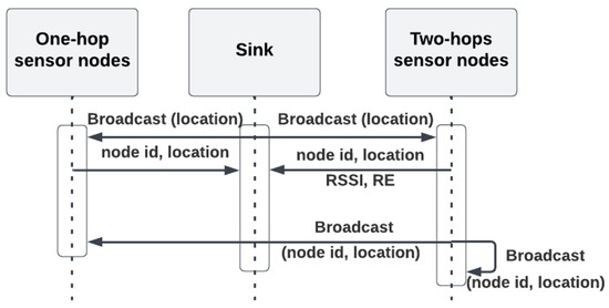
Figure 1. Sequence diagram of the initialization phase.

Following these steps in the network deployment and initialization phase, the WBAN achieves an organized and coordinated setup. The information shared between the sink node and sensor nodes, along with the exchange of information among the two-hop nodes, establishes a foundation for effective communication and data transfer. This initialization phase ensures that the network is properly configured and ready for the subsequent data transmission and routing stages. Additionally, this phase in WBAN is designed to minimize the overhead in communication cost, further discussed in Section 5. In this case, data forwarding and routing decisions can be performed by giving the sink node essential information from the two-hop sensor nodes (i.e., location, RSSI, and residual energy). Through efficient assignment of parent nodes, the network reduces unnecessary communication overhead. This minimization of overhead conserves energy resources and enhances the overall efficiency and reliability of data transmission in WBAN. By striving to minimize the communication cost overhead, the network deployment and initialization phase lays the foundation for an optimized and energy-efficient WBAN system.

4.2.2. Parent Node Selection

After the sink node receives the necessary information from the sensor nodes, it employs a cost function to select the parent nodes. The cost function considers factors such as the distance between a sensor node and the sink, the current residual energy level of the node, and the RSSI value from a sensor node to the sink. The distance between the sink and the sensor node is calculated using the Euclidean formula, while the residual energy is determined as discussed in Section 3.2. The RSSI value, which follows a log-normal distribution, further discussed in Section 5.1, is updated for each transmission. Hence, the cost function, denoted as $CF\left(i\right)$ for the sensor node i, is calculated as Equation (7), where d represents the distance between node i and the sink, $RE\left(i\right)$ is the residual energy, and $RSSI\left(i\right)$ indicates the RSSI value of node i.

$$CF\left(i\right)=\frac{d\times RSSI\left(i\right)}{RE\left(i\right)}$$

(7)

By incorporating distance, the cost function considers the physical proximity of each sensor node to the sink node. Including residual energy in the cost function is significant for energy efficiency. Nodes with higher residual energy levels are given high scores, indicating their ability to handle data-forwarding tasks. Additionally, the cost function incorporates RSSI values, which reflect the signal quality between the nodes and the sink. The algorithm prioritizes nodes with stronger and more reliable communication links by considering RSSI. This balanced distribution of responsibilities helps prevent energy imbalance among nodes and contributes to the network’s longevity.

In particular, the sink node selects the parent node based on several criteria, including shorter distance, higher RSSI value, and greater residual energy. Once the cost function is computed for all two-hop sensor nodes, the sink node selects the parent node with the maximum cost function value. However, there is a constraint on the number of nodes that a parent node can serve ($\tau$). This constraint ensures optimal utilization of resources within the network.

The selection of parent nodes is an ongoing process that adapts to the changing energy levels of the sensor nodes. When the energy of a selected parent node reaches a threshold value ($Th$), the sink stops using this node for forwarding packets. At that time, another node has been selected as a parent node, as previously explained. Once the residual energy of all two-hop sensor nodes reaches the threshold ($Th$), a new round of parent node selection is initiated. In this case, all two-hop sensor nodes can serve as parent nodes. This approach ensures that the flow of traffic and data routing within the WBAN remains efficient and well-balanced. After selecting the parent nodes, their identifiers are broadcast to all two-hop sensor nodes, enabling them to establish a communication link with their designated parent node. It is important to note that reaching the energy threshold value ($Th$) is an alarm, signaling the network management system to replace or recharge the node.

By selecting the parent nodes based on the maximum cost function value, the threshold energy value ($Th$), and the limitation in the number of nodes that the parent node can serve ($\tau$), the algorithm redistributes the data traffic among the sensor nodes. This strategy prevents any single node from becoming overwhelmed with excessive data forwarding responsibilities, promoting a greater utilization of network resources. In this scenario, the lifetime of all sensor nodes is extended, and the energy consumption is more evenly distributed throughout the network. The pseudo-code of the parent node selection process is depicted in Algorithm 1, while the flowchart for this process is shown in Figure 2.

Algorithm 1 Parent Node Selection Process

Input:  N (Number of nodes), d[1..N] (distances from sensor nodes to the sink), RE[1…N] (residual energy levels of sensor nodes), RSSI[1..N] (RSSI values of sensor nodes), τ (number of serving nodes for parent node), Th (energy threshold), one-hop nodes’ id Output:  $PN$ (Parent nodes’ id) 1: for$i=1$ to N do 2:     if i not in one-hop nodes’ id then 3: $CF\left[i\right]=\frac{d\left[i\right]\times RSSI\left[i\right]}{RE\left[i\right]}$              ▹ Cost Function 4:     end if 5: end for 6: $serv{e}_{count}[1..N]=0$ 7: $SortedCF=Sort\left(CF\right)$                    ▹ Ascending Sorting 8: $indices[1..N]=0$ 9: for $i=1$ to N do         ▹ Store indices of nodes after sorting cost function 10: $indices\left[i\right]=IndexOf(CF,SortedCF[i\left]\right)$    ▹ Get indices of nodes after sorting 11: end for 12: for $j=1$ to N do                      ▹ Static Clustering 13:     for i in $indices$ do 14:         if $serv{e}_{count}\left[i\right]<\tau$ and $RE\left[i\right]>0$ and $RE\left[i\right]>Th$ then 15:            if $i!=j$ then 16: $serv{e}_{count}\left[i\right]+=1$ 17:            end if 18: $index=i$ 19:         end if 20:     end for 21: $PN\left[j\right]=index$ 22: end for 23: if $RE[1..N]<=Th$ then                 ▹ Dynamic Clustering 24:     for $j=1$ to N do 25:         for i in $indices$ do 26:            if $serv{e}_{count}\left[i\right]<\tau$ and $RE\left[i\right]>0$ and $RE\left[i\right]<=Th$ then 27:                if $i!=j$ then 28: $serv{e}_{count}\left[i\right]+=1$ 29:                end if 30: $index=i$ 31:            end if 32:         end for 33: $PN\left[j\right]=index$ 34:     end for 35: end if

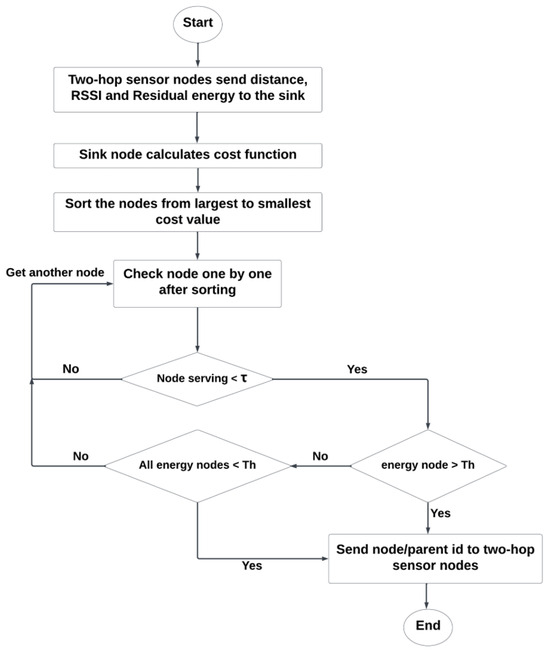
Figure 2. Flowchart of the parent node selection process.

4.2.3. Data Transmission

After the parent node selection and network organization, the WBAN enters the data transmission phase. This phase considers the specific requirements of one-hop sensor nodes, which transmit their critical data directly to the sink. Meanwhile, two-hop sensor nodes transmit their packets to the chosen parent node before reaching the sink node.

After each round of data transmission, the two-hop sensor nodes send their updated residual energy (RE) and RSSI values to the sink. This information is used to update the cost function calculations and, consequently, to select the parent nodes. During this process, the sink actively monitors the residual energy level of the parent node. If the parent node’s residual energy reaches a threshold ($Th$), the sink temporarily suspends its involvement in data forwarding until the residual energy of all two-hop sensor nodes reaches the threshold ($Th$). At that moment, the sink node selects another two-hop sensor node as a parent node. This ensures that no individual parent node becomes excessively drained of energy, maintaining a balanced traffic load distribution and prolonging the overall network stability.

Upon reaching the threshold energy level for all two-hop sensor nodes, a new round of parent node selection is initiated. At this stage, all two-hop sensor nodes are eligible to serve as parent nodes and participate in data forwarding. This approach promotes fairness by giving each two-hop sensor node an opportunity to contribute as a parent node, which in turn extends the lifetime of the network as a whole. The sequential steps and the pseudo-code of the data transmission phase are shown in Figure 3 and Algorithm 2, respectively.

Algorithm 2 Data Transmission

Input:  N (Number of nodes), R (Number of rounds), PN[1…N] (parent node), E[1…N] (initial node energy), Etx (transmitted energy consumption as in Equation (1), Erx (received energy consumption as in Equation (2), one-hop nodes’ id. Output:  Transmission of all node packets to the sink (single-hop, two-hop) 1: for $round=1$ to R do 2:     for $i=1$ to N do 3:         if i in one-hop nodes’ id then                ▹ Critical Packet 4:            if $E\left[i\right]>0$ then                     ▹ Enough Energy 5:                   Send packet directly to the sink 6: $E\left[i\right]=E\left[i\right]-E_{tx}$ 7:            else                         ▹ Not Enough Energy 8:                   Cannot send the packet 9:            end if 10:         else                           ▹ Normal Packet 11:            if $E\left[i\right]>0$ then                    ▹ Enough Energy 12:                   Send packet to $PN\left[i\right]$ 13: $E\left[i\right]=E\left[i\right]-E_{tx}$ 14: $E\left[PN\left[i\right]\right]=E\left[PN\left[i\right]\right]-E_{rx}$ 15:                   Send packet from $PN\left[i\right]$ to the sink 16: $E\left[PN\left[i\right]\right]=E\left[PN\left[i\right]\right]-E_{tx}$ 17:            else                        ▹ Not Enough Energy 18:                   Cannot send the packet 19:            end if 20:         end if 21:     end for 22: end for

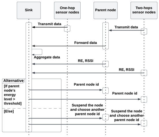
Figure 3. Sequence diagram of the data transmission phase.

4.3. Time Complexity

We first analyze the time complexity of Algorithm 1 (i.e., the parent node selection process) and Algorithm 2 (i.e., data transmission), and then we combine the time complexities of both algorithms to obtain the overall time complexity for our proposed protocol.

1.

Parent node selection process: This algorithm aims to select appropriate parent nodes for transmitting the data from the two-hop sensor node to the selected parent node and then relaying it to the sink. This algorithm runs on the sink node and involves the following steps:

(a)

Calculating the cost function for all two-hop sensor nodes at the sink node. This step has a time complexity of $O\left(N\right)$, where N represents the number of nodes in the network (lines 1 to 5 in Algorithm 1);

(b)

Sorting the nodes based on their cost function values. The sorting operation has a time complexity of $O(Nlog(N\left)\right)$ (line 7 in Algorithm 1), using merge-sorting;

(c)

Storing the indices of the sorted nodes requires $O\left(N\right)$ time complexity (lines 9 to 11 in Algorithm 1);

(d)

Iterating through the sorted nodes to select those serving a limited number of nodes and having sufficient energy for packet transmission. This process includes both static clustering (lines 12 to 22 in Algorithm 1) and dynamic clustering (lines 23 to 35 in Algorithm 1) parts. This step is applied to each two-hop sensor node. Thus, the time complexity of these iterations has a maximum of $O\left(N^2\right)$.

By summing up the time complexities of these steps, the overall time complexity of the parent node selection algorithm is $O\left(N\right)+O(Nlog\left(N\right))+O\left(N\right)+O\left(N^2\right)$, which can be simplified to $O\left(N^2\right)$.

2.

Data transmission: This algorithm transmits data from the sensor node to the sink node. If a node sends a critical packet with sufficient energy, it transmits it directly to the sink (lines 3 to 6 in Algorithm 2). However, when a node sends a normal packet with enough energy, it sends the packet to its parent node, which the sink node chooses. The parent node then forwards the packet to the sink (lines 10 to 16 in Algorithm 2). The steps include:

(a)

Iterating through all N nodes in the network for varying rounds R. This operation has a time complexity of $O\left(RN\right)$.

By combining the time complexities of both algorithms, the total time complexity of our proposed protocol is $O\left(N^2\right)+O\left(RN\right)$. Since the dominant term is $O\left(N^2\right)$, we can express the overall time complexity as $O\left(N^2\right)$.

Regarding space complexity, the algorithm mainly requires memory for storing network information, such as node indices, locations, energy levels, RSSI, and any additional data structures used for sorting and calculations. The space complexity depends on the number of nodes and the size of the data structures, but it is typically within reasonable bounds for most WBAN applications.

5. Simulation Results and Analysis

We carried out a series of experiments to evaluate the performance of our proposed protocol, HCEL. Details regarding the performance metrics can be found in Section 3.4. The evaluation involved comparing our proposed protocol (HCEL) with both SIMPLE and ERRS protocols [24,25] across these performance metrics. Our implementation utilized the Networkx package [69] with different experiment parameters outlined in Table 3. To account for the inherent randomness in the RSSI values generated by our protocol, we conducted 15 simulation runs following a log-normal distribution, each lasting 35,000 time units.

Table 3. Experimental parameters.

Parameters	Value
Initial energy of the sensors	4 joules
Number of sink nodes	1
Number of sensor nodes	10
Packet size $\left(k\right)$	127 bytes
Reference distance $\left(d_0\right)$	10 cm
Frequency $\left(f\right)$	2.4 GHz
Path loss coefficient $\left(\eta \right)$	3.38
Standard deviation $\left(\sigma \right)$	4.1 dB
Mean $\left(\mu \right)$	0
Energy threshold ($Th$)	2 joules
Number of serving nodes for parent node ($\tau$)	4
Total number of rounds (R)	35,000

5.1. Experimental Testbed Setup

Our experimental testbed was established within an academic unit’s laboratory. The network topology in our testbed comprises 10 sensors, denoted as node 1 through node 10, and a central sink node identified as node 0. The system structure of our network is illustrated in Figure 4. To collect data from sensor nodes, we employed Crossbow MICAz motes running the TinyOS embedded operating system in our testbed, each equipped with a 1.2-inch-long monopole antenna with a wavelength of one-quarter inch. These motes were programmed to transmit sensing (i.e., physiological) data to the sink node at 3-min intervals. Communication among the nodes was established using the Chipcon CC2420 (Chipcon, Oslo, Norway) transceiver operating at 2.4 GHz, which facilitates data exchange among sensors.

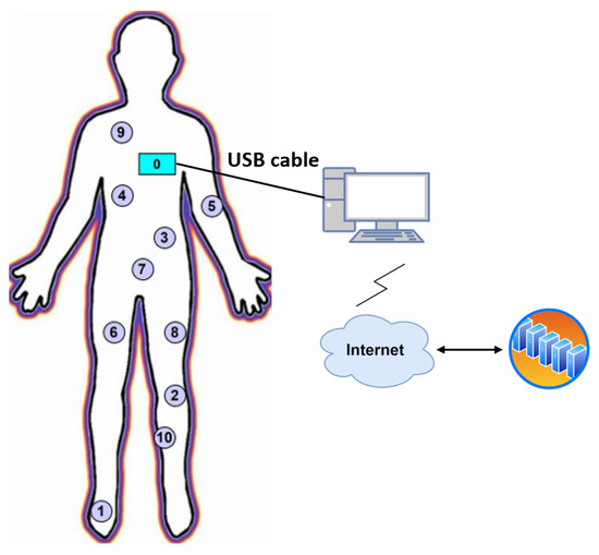
Figure 4. System architecture.

In our network, the sink node (node 0) serves as the gateway, receiving data from the sensors and relaying it to the backend servers. This sink node utilizes USB connectivity to establish communication with the cloud, facilitate configuration, and supply power. Therefore, it could be connected to any PC using a USB cable, as shown in Figure 4. All sensor nodes, except the sink node, were powered by AA batteries and had sufficient power (i.e., RSSI) to communicate with each other and the sink node. The transmission power in our testbed was configured within the range of 0 dBm (1 mW) to $-25$ dBm (0.003 mW) to minimize interference and conserve radio power consumption. The primary objective of this testbed was to assess the performance of the WBAN and gather additional data for future investigations.

In wireless networks, high RSSI values indicate reliable data transfer capabilities. Thus, our work leveraged the data collected from the sensor nodes in our testbed to model RSSI using a log-normal distribution. The choice of log-normal distribution was validated through a goodness-of-fit assessment using a QQ-plot, confirming its suitability for our data as shown in Figure 5. The log-normal distribution, widely applied in this domain, offers a probability density function (PDF) that effectively characterizes the distribution of RSSI values. By adopting this approach, we gain a deeper understanding of RSSI behavior and its implications within our work.

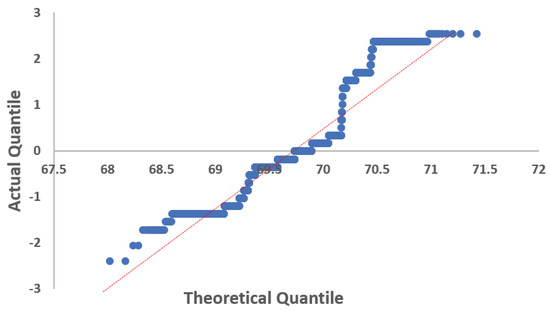
Figure 5. QQ–plot.

5.2. Node Deployment

In our simulation setup, we strategically positioned sensors on the human body, as shown in Figure 6. Among these sensors, one-hop nodes, such as sensor 3 and sensor 7, are crucial in monitoring tasks that require immediate action (e.g., ECG and glucose). Due to their critical nature and time-sensitive requirements, these sensors transmit their data to the sink (node 0) using single-hop communication, as illustrated in Figure 6 (e.g., direct packet transmission from node 3 to node 0). These critical sensors are positioned near the sink node to ensure efficiency and prompt data delivery.

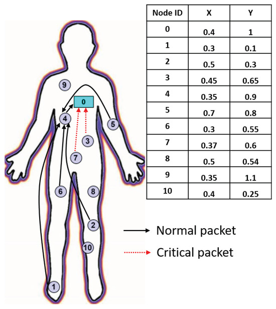
Figure 6. Node deployment.

On the other hand, the two-hop sensor nodes are responsible for normal monitoring functions, encompassing all other deployed sensor nodes shown in Figure 6. These nodes adopt a two-hop communication approach, transmitting their data through the intermediate parent node to reach the sink. The transmission path of packets from some two-hop sensor nodes to the sink is showcased in Figure 6 (e.g., packet transmission from sensor node 1 to node 4, the selected parent node, and then to node 0, the sink node). Using a two-hop communication extends the network lifetime by distributing the energy consumption among nodes, reducing the distance to the sink, and mitigating the energy drain on any single sensor. This design choice ensures a balance between critical monitoring requirements and the efficient utilization of network resources for normal monitoring tasks.

In the experiment depicted in Figure 7 and Figure 8, we compared the network lifetime and stability period of our proposed routing protocol (HCEL) with both SIMPLE and ERRS protocols. The results demonstrate the superiority of the HCEL protocol in extending both the stability period and the overall network lifetime. The effectiveness of our proposed protocol stems from selecting parent nodes based on residual energy (i.e., not exceeding the threshold value $Th$), ensuring that the energy load is evenly distributed across the network and providing the chance for every sensor node to become a parent node. In contrast, the low performance of the SIMPLE protocol arises from the repeated selection of nodes closer to the sink as parent nodes, leading to their quick energy depletion and subsequent death of other sensor nodes. While the ERRS protocol does improve network lifetime compared to SIMPLE, it still falls short of the performance achieved by our HCEL protocol. ERRS achieves this improvement by balancing the load and selecting a new parent node after a set number of transmission rounds. Moreover, ERRS considers both distance and residual energy when selecting parent nodes. However, our HCEL protocol takes it a step further by considering an additional parameter, RSSI from the node to the sink, to make better parent node selections. This additional refinement helps optimize energy usage and contributes to the high performance of our protocol.

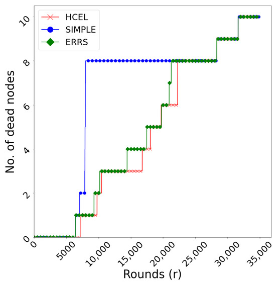
Figure 7. Analysis of network lifetime.

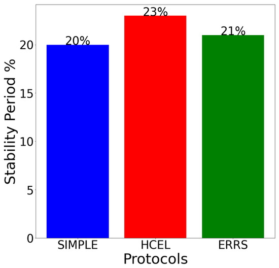
Figure 8. Comparing the stability period among the HCEL, SIMPLE, and ERRS protocols.

We observed the number of dead nodes over different rounds to evaluate the network lifetime, as shown in Figure 7. The results indicate the higher performance of our proposed routing protocols compared to both the SIMPLE and ERRS protocols. Our protocol increases the stability period, with the HCEL protocol achieving approximately 7300 rounds, surpassing the 6383 rounds attained by the SIMPLE protocol and the 6425 rounds achieved by the ERRS protocol. Additionally, in both HCEL and ERRS protocols, two-hop sensor nodes exhibit extended lifetimes due to the balanced distribution of traffic load. This achievement is made possible by combining static and dynamic clustering during the parent node selection process; thus, the stability period and network lifetime increase. Notably, nodes 3 and 7 in all protocols, which do not participate in data forwarding or routing, exhibit longer lifetimes, as their communication is direct to the sink (i.e., the last two dead nodes).

In the stability period experiment, we focus on the duration from network initiation until the first node’s depletion for our proposed protocol (HCEL), along with the SIMPLE and ERRS protocols. From Figure 8, our proposed protocol achieves a stability period of 23% of the total operational duration, slightly surpassing both the ERRS protocol at 21% and the SIMPLE protocol at 20%. These results highlight the effectiveness of our proposed protocol in providing a longer stability period, indicating an extension in the lifetimes of nodes beyond the first node’s depletion.

The next experiment, shown in Figure 9, Figure 10 and Figure 11, evaluates the network throughput based on the number of packets successfully received at the sink, the packet delivery ratio (PDR), and the number of dropped packets. To demonstrate the superior performance of our proposed routing protocol (HCEL), we compared the results with both the SIMPLE and ERRS protocols, aiming to establish its maximum throughput advantage.

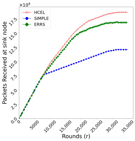
Figure 9. Analysis of total number of packets successfully received at the sink.

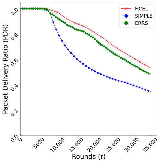
Figure 10. Analysis of packet delivery ratio (PDR).

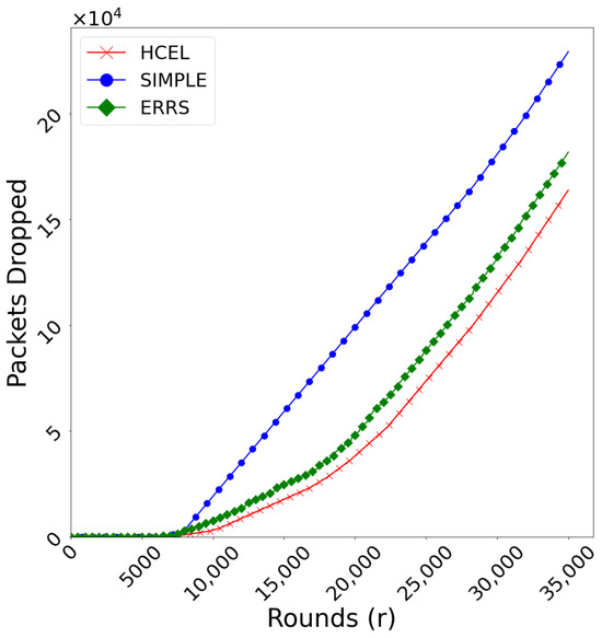
Figure 11. Analysis of total number of dropped packets.

Figure 9 depicts the number of packets successfully delivered to the sink node in different rounds. When there are no dead nodes in all protocols (i.e., from round 0 until round 6383), the sink node receives the same number of packets sent. However, as nodes in the network become inactive or die, the number of received packets at the sink decreases. The delivery of packets to the sink depends on the number of active or alive nodes in the network. Therefore, more alive nodes lead to more data packets to the sink, ultimately maximizing network throughput. Due to the extended lifetimes of sensor nodes in our protocol (HCEL), the number of packets received at the sink is larger than that of the SIMPLE and ERRS protocols. The gap between the HCEL and SIMPLE protocols increases as the number of rounds increases. This occurs because the SIMPLE protocol quickly loses its nodes after the first node’s depletion, causing a decrease in the number of received packets at the sink. However, the difference between the HCEL and ERRS is less pronounced due to the extended network lifetime observed in the ERRS protocol.

Figure 10 shows the packet delivery ratio (PDR) across various rounds. PDR represents the ratio of packets successfully delivered to the sink to the total number of transmitted packets. As our protocol (HCEL) successfully delivers a larger number of packets to the sink, it exhibits higher throughput regarding PDR compared to both the SIMPLE and ERRS protocols. The superiority of our protocol and ERRS protocol can be attributed to its longer stability period resulting from uniform load distribution and increased lifetime of sensor nodes. However, our protocol’s performance surpasses that of the ERRS protocol, due to its consideration of the RSSI between the node and sink during parent node selection. When $PDR=1$, all packets were received successfully to the sink. However, as $PDR$ decreases, the number of packets dropped increases.

Figure 11 illustrates that the number of dropped packets in the HCEL is lower than in the ERRS and SIMPLE protocols. This is due to the longer stability period of our protocol and to the consideration of different parameters when selecting the parent node. In particular, during the stability period, when all nodes are alive, no packets are dropped. The increase in the number of dead nodes and the speed of depletion of nodes influence the total number of packets dropped in different rounds.

We measure the average residual energy of 10 nodes across different rounds in our next experiment, shown in Figure 12. Since the initial energy of each node is 4 joules, the average energy in round 0 is 4 joules. The simulation runs until all deployed sensor nodes exhaust their energy (i.e., RE = 0). Figure 12 depicts the decrease in the residual energy of all deployed nodes as the rounds progress. In the SIMPLE protocol, the residual energy of sensor nodes is drastically reduced after the first node dies (at round 6383). This rapid reduction occurs due to the speed at which all other nodes deplete their energy after the death of the first node. However, our proposed protocol (HCEL) and the ERRS protocol outperform the SIMPLE protocol, especially after the depletion of the first node. The better performance of our proposed and ERRS protocols is due to the use of a static and dynamic clustering-based routing mechanism. By allowing every sensor node to become a parent node, the load is evenly distributed among all nodes, extending their lifetime. Furthermore, the efficient selection of parent nodes and appropriate route selection in our proposed scheme (HCEL) play a significant role in the energy conservation of the deployed sensor nodes, thus extending the network lifetime compared to both the ERRS and SIMPLE protocols.

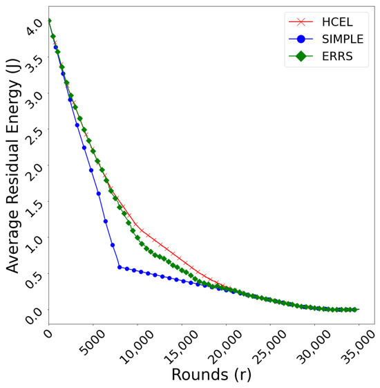
Figure 12. Analysis of residual energy.

The experiment in Figure 13 calculates an average EED for our proposed protocol (HCEL), as well as the SIMPLE and ERRS protocols. The results, shown in Figure 13, indicate that our proposed protocol achieves a lower delay than the SIMPLE and ERRS protocols. The key factor contributing to the improved EED in our protocol lies in the use of an adaptive static cluster routing mechanism, coupled with the careful selection of the parameters during parent node selection. That is, unlike the frequent selection of nodes closest to the sink as parent nodes in the SIMPLE protocol, our approach ensures a more balanced distribution of the traffic load among the nodes. This measure effectively mitigates rapid energy depletion at specific nodes, thereby enhancing the successful reception of packets at the sink and reducing the overall delay. As a result, our protocol shows an impressive improvement of approximately 56% compared to the SIMPLE protocol and approximately 40% compared to the ERRS protocol.

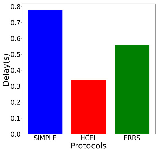
Figure 13. Comparing the end-to-end delay among the HCEL, SIMPLE, and ERRS protocols.

The following experiment, shown in Figure 14, analyzes the network cumulative path loss for our proposed protocol (HCEL), as well as for the SIMPLE and ERRS protocols. Using two-hop transmission in the routing protocol helps minimize the data transmission distance from the sensor nodes to the sink, resulting in lower path loss. Initially, our proposed protocol (HCEL) and ERRS protocol perform well compared to the SIMPLE protocol. However, starting from round 7981, all two-hop sensor nodes in the SIMPLE protocol deplete their energy, leading to a significant decrease in path loss. Consequently, the SIMPLE protocol exhibits a greater reduction in path loss compared to our proposed protocol (HCEL) and to the ERRS protocol from round 7981 to round 22,268. It is worth noting that the cumulative path loss is minimal when the number of alive nodes is minimal. Additionally, the increase in path loss observed in our proposed protocol (HCEL) and ERRS protocol during this period (rounds 6383 to 22,268) is due to its longer stability period and a higher number of alive nodes, contributing to the increased cumulative path loss.

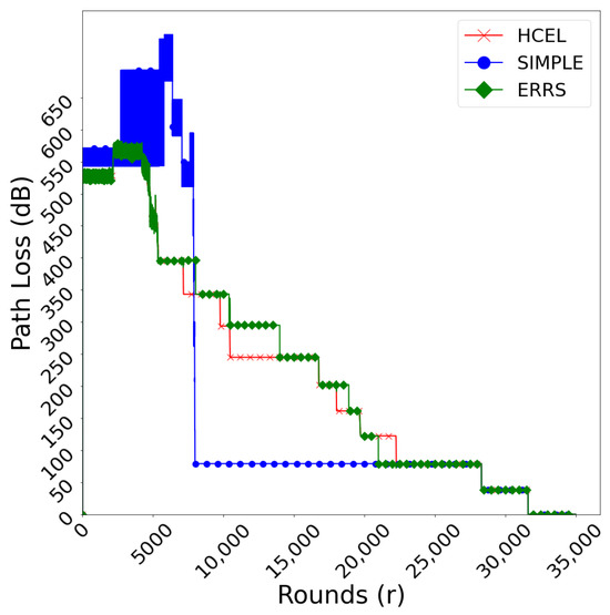
Figure 14. Analysis of network path loss.

To address the overhead issue, efficient routing protocols aim to reduce the size of control packets. In our experiment, depicted in Figure 15, we analyze the communication cost in terms of bits for various numbers of rounds for our proposed protocol (HCEL), as well as for the SIMPLE and ERRS protocols. While the payload size remains the same (127 bytes) in all protocols, the difference lies in the overhead calculation. In the HCEL protocol, the overhead during the initialization phase in round 0 (63,424 bits) is lower compared to the SIMPLE protocol (94,080 bits). This is because one-hop sensor nodes do not participate in data forwarding or routing, eliminating the need to send their energy levels and RSSI values to other nodes or the sink in our protocol. After each round of data transmission, our protocol only sends the unique identifier of the respective parent node to two-hop sensor nodes, without requiring the transmission of the cost function to all nodes for parent node selection, as done in the SIMPLE protocol. Furthermore, one-hop sensor nodes in our protocol do not need to send their updated residual energy to the sink for cost function calculation, as required in the SIMPLE protocol. However, in the ERRS protocol, the overhead during the initialization phase is 53,281 bits, which is less than in our HCEL protocol. This discrepancy occurs because nodes in the ERRS protocol transmit only their residual energy to the sink node during initialization, whereas in the HCEL protocol, they transmit both residual energy and RSSI values. This leads to an increase in the number of bits during the initialization phase in the HCEL protocol. Additionally, after each data transmission round in the HCEL protocol, all nodes must send their updated residual and RSSI to the sink node to calculate the cost value and then choose the appropriate parent node. Conversely, in the ERRS protocol, nodes only send updated residual energy to select the parent node, resulting in a decrease in communication cost across different rounds compared to our HCEL protocol.

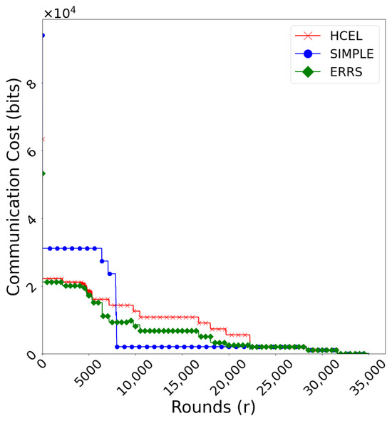
Figure 15. Analysis of network communication cost.

It is observable that the SIMPLE protocol generates a smaller number of bits for communication from rounds 7981 to 22,268 compared to the HCEL and ERRS protocols. That is because no two-hop sensor nodes are still alive for any communication. However, when all protocols have the same number of alive nodes, ERRS and our proposed protocol (HCEL) require fewer bits for communication between sensor nodes and the sink, as in the case from rounds 0 to 6383. This reduction in communication cost is attributed to the optimized overhead calculation and efficient exchange mechanisms employed in our proposed protocol. By optimizing these aspects, our protocol reduces communication costs between sensor nodes and the sink compared to the SIMPLE protocol.

ETX is calculated, as discussed in Section 3.4.7, to measure the link quality of our proposed protocol (HCEL), as well as the SIMPLE and ERRS protocols in different rounds. In Figure 16, it can be seen that, when all sensor nodes are operational for all protocols, the ETX value stands at 1. This implies that no packets are lost and that every packet is successfully transmitted to the sink. However, as the packet loss between nodes increases, the ETX value also increases. The ETX values in the SIMPLE protocol are larger than those of our proposed protocol (HCEL) and ERRS protocol, especially after round 7300 for HCEL and after round 6425 for ERRS. This indicates that the link quality in the SIMPLE protocol is poorer compared to both the HCEL and ERRS protocols. In general, as the number of rounds increases, the gap in ETX values between our protocol and SIMPLE widens, referring to a larger number of successfully received packets in the HCEL protocol compared to the SIMPLE protocol. However, this gap narrows between the HCEL and ERRS protocols due to the improved network lifetime observed in the ERRS protocol compared to the SIMPLE protocol.

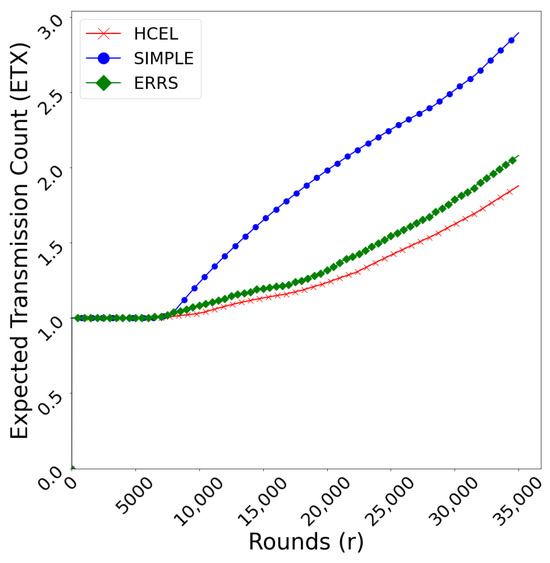
Figure 16. Analysis of expected transmission count (ETX).

6. Conclusions

In this paper, we present HCEL, a novel, energy-efficient, and reliable routing protocol specifically designed to enhance the overall performance of WBANs. By integrating static and dynamic clustering routing techniques in the parent node selection process, HCEL significantly improves the stability period and extends network lifetimes, thereby maximizing the reliability of WBANs. By conducting thorough simulations using Networkx, we provide empirical evidence showcasing the superiority of HCEL over both the SIMPLE and ERRS protocols across various performance metrics. HCEL substantially enhances network stability periods, network lifetimes, throughput, residual energy, path loss, and expected transmission counts. Particularly noteworthy is the remarkable 56% and 40% reduction in end-to-end delay achieved by HCEL compared to the SIMPLE and ERRS protocols, respectively, highlighting its efficiency and reliability as a routing solution for WBANs. To further advance the capabilities and applications of WBANs in healthcare and beyond, our future work will focus on incorporating mobility and security considerations. By addressing these key issues, we can further enhance the versatility and robustness of WBANs, enabling their effective deployment in a wide range of real-world scenarios.

References

- Available online: https://data.worldbank.org/ (accessed on 8 June 2023).
- Available online: https://www.zawya.com/en/uae (accessed on 8 June 2023).
- Sahndhu, M.M.; Javaid, N.; Imran, M.; Guizani, M.; Khan, Z.A.; Qasim, U. BEC: A novel routing protocol for balanced energy consumption in wireless body area networks. In Proceedings of the 2015 International Wireless Communications and Mobile Computing Conference (IWCMC), Dubrovnik, Croatia, 24–28 August 2016; pp. 653–658. [Google Scholar]
- Shu, M.M.; Javaid, N.; Akbar, M.; Najeeb, F.; Qasim, U.; Khan, Z.A. FEEL: Forwarding data energy efficiently with load balancing in wireless body area networks. In Proceedings of the 2014 IEEE 28th International Conference on Advanced Information Networking and Applications, Victoria, BC, Canada, 13–16 May 2014; pp. 783–789. [Google Scholar]
- Ullah, Z.; Ahmed, I.; Razzaq, K.; Naseer, M.K.; Ahmed, N. DSCB: Dual sink approach using clustering in body area network. Peer Peer Netw. Appl. 2019, 12, 357–370. [Google Scholar] [CrossRef]
- Ahmed, S.; Javaid, N.; Yousaf, S.; Ahmad, A.; Shu, M.M.; Imran, M.; Khan, Z.A.; Alrajeh, N. Co-LAEEBA: Cooperative link aware and energy efficient protocol for wireless body area networks. Comput. Hum. Behav. 2015, 51, 1205–1215. [Google Scholar] [CrossRef]
- Cavallari, R.; Martelli, F.; Rosini, R.; Buratti, C.; Verdone, R. A survey on wireless body area networks: Technologies and design challenges. IEEE Commun. Surv. Tutor. 2014, 16, 1635–1657. [Google Scholar] [CrossRef]
- Goyal, R.; Mittal, N.; Gupta, L.; Surana, A. Routing protocols in wireless body area networks: Architecture, challenges, and classification. Wirel. Commun. Mob. Comput. 2023, 2023, 9229297. [Google Scholar] [CrossRef]
- Khan, J.Y.; Yuce, M.R.; Bulger, G.; Harding, B. Wireless body area network (WBAN) design techniques and performance evaluation. J. Med. Syst. 2012, 36, 1441–1457. [Google Scholar] [CrossRef]
- Chen, M.; Gonzalez, S.; Vasilakos, A.; Cao, H.; Leung, V.C. Body area networks: A survey. Mob. Networks Appl. 2011, 16, 171–193. [Google Scholar] [CrossRef]
- Ghamari, M.; Janko, B.; Sherratt, R.S.; Harwin, W.; Piechockic, R.; Soltanpur, C. A survey on wireless body area networks for ehealthcare systems in residential environments. Sensors 2016, 16, 831. [Google Scholar] [CrossRef] [PubMed]
- Latré, B.; Braem, B.; Moerman, I.; Blondia, C.; Demeester, P. A survey on wireless body area networks. Wirel. Netw. 2011, 17, 1–18. [Google Scholar] [CrossRef]
- Movassaghi, S.; Abolhasan, M.; Lipman, J.; Smith, D.; Jamalipour, A. Wireless body area networks: A survey. IEEE Commun. Surv. Tutor. 2014, 16, 1658–1686. [Google Scholar] [CrossRef]
- Muhannad, Q.; Biswas, S. On-body packet routing algorithms for body sensor networks. In Proceedings of the 2009 First International Conference on Networks & Communications NetCoM (2009), Chennai, India, 27–29 December 2009; pp. 171–177. [Google Scholar]
- Ullah, S.; Khan, P.; Ullah, N.; Saleem, S.; Higgins, H.; Kwak, K.S. A review of wireless body area networks for medical applications. arXiv 2010, arXiv:1001.0831. [Google Scholar] [CrossRef]
- Cornet, B.; Fang, H.; Ngo, H.; Boyer, E.W.; Wang, H. An overview of wireless body area networks for mobile health applications. IEEE Netw. 2022, 36, 76–82. [Google Scholar] [CrossRef]
- Hasan, K.; Biswas, K.; Ahmed, K.; Nafi, N.S.; Islam, M.S. A comprehensive review of wireless body area network. J. Netw. Comput. Appl. 2019, 143, 178–198. [Google Scholar] [CrossRef]
- Wu, T.; Wu, F.; Redoute, J.M.; Yuce, M.R. An autonomous wireless body area network implementation towards IoT connected healthcare applications. IEEE Access 2017, 5, 11413–11422. [Google Scholar] [CrossRef]
- Qu, Y.; Zheng, G.; Ma, H.; Wang, X.; Ji, B.; Wu, H. A survey of routing protocols in WBAN for healthcare applications. Sensors 2019, 19, 1638. [Google Scholar] [CrossRef] [PubMed]
- Crosby, G.V.; Ghosh, T.; Murimi, R.; Chin, C.A. Wireless body area networks for healthcare: A survey. Int. J. Hoc, Sens. Ubiquitous Comput. 2012, 3, 1–26. [Google Scholar] [CrossRef]
- Elhadj, H.B.; Chaari, L.; Kamoun, L. A survey of routing protocols in wireless body area networks for healthcare applications. Int. J. Health Med. Commun. 2012, 3, 1–18. [Google Scholar] [CrossRef]
- Ahmed, S.; Javaid, N.; Akbar, M.; Iqbal, A.; Khan, Z.A.; Qasim, U. LAEEBA: Link aware and energy efficient scheme for body area networks. In Proceedings of the 2014 IEEE 28th International Conference on Advanced Information Networking and Applications AINA (2014), Victoria, BC, Canada, 13–16 May 2014; pp. 435–440. [Google Scholar]
- Javaid, N.; Ahmad, A.; Nadeem, Q.; Imran, M.; Haider, N. iM-SIMPLE: iMproved stable increased-throughput multi-hop link efficient routing protocol for Wireless Body Area Networks. Comput. Hum. Behav. 2015, 51, 1003–1011. [Google Scholar] [CrossRef]
- Nadeem, Q.; Javaid, N.; Mohammad, S.N.; Khan, M.Y.; Sarfraz, S.; Gull, M. Simple: Stable increased-throughput multi-hop protocol for link efficiency in wireless body area networks. In Proceedings of the 2013 Eighth International Conference on Broadband and Wireless Computing, Communication and Applications, Compiegne, France, 28–30 October 2013; pp. 221–226. [Google Scholar]
- Ullah, F.; Khan, M.Z.; Faisal, M.; Rehman, H.U.; Abbas, S.; Mubarek, F.S. An energy efficient and reliable routing scheme to enhance the stability period in wireless body area networks. Comput. Commun. 2021, 165, 20–32. [Google Scholar] [CrossRef]
- Wang, F.; Hu, F.; Wang, L.; Du, Y.; Liu, X.; Guo, G. Energy-efficient medium access approach for wireless body area network based on body posture. China Commun. 2015, 12, 122–132. [Google Scholar] [CrossRef]
- Wang, F.; Hu, F.; Wang, L.; Du, Y.; Liu, X. Posture-aware medium access approach under walking scenery for wireless body area network. In Proceedings of the 2014 IEEE International Conference on Communication Systems, Macau, China, 19–21 November 2014; pp. 457–461. [Google Scholar]
- Gaikwad, V.D.; Ananthakumaran, S. A Review: Security and Privacy for Health Care Application in Wireless Body Area Networks. Wirel. Pers. Commun. 2023, 130, 673–691. [Google Scholar] [CrossRef]
- Saba, T.; Haseeb, K.; Ahmed, I.; Rehman, A. Secure and energy-efficient framework using Internet of Medical Things for e-healthcare. J. Infect. Public Health 2020, 13, 1567–1575. [Google Scholar] [CrossRef] [PubMed]
- Wu, L.; Zhang, Y.; Li, L.; Shen, J. Efficient and anonymous authentication scheme for wireless body area networks. J. Med. Syst. 2016, 40. [Google Scholar] [CrossRef] [PubMed]
- He, Z.G.; Chung, C.; Poon, Y.; Zhang, Y.T. A review on body area networks security for healthcare. Int. Sch. Res. Not. 2011, 2011, 692592. [Google Scholar]
- Fayaz, A.; Rehmani, M.H. Energy harvesting for self-sustainable wireless body area networks. IT Prof. 2017, 19, 32–40. [Google Scholar]
- Lu, G.; Sadagopan, N.; Krishnamachari, B.; Goel, A. Delay efficient sleep scheduling in wireless sensor networks. In Proceedings of the IEEE 24th Annual Joint Conference of the IEEE Computer and Communications Societies, Miami, FL, USA, 13–17 March 2005; pp. 2470–2481. [Google Scholar]
- Ruzzelli, A.G.; Jurdak, R.; O’Hare, G.M.; Van Der Stok, P. Energy-efficient multi-hop medical sensor networking. In Proceedings of the 1st ACM SIGMOBILE International Workshop on Systems and Networking Support for Healthcare and Assisted Living Environments, San Juan, Puerto Rico, 11 June 2007; pp. 37–42. [Google Scholar]
- Mehdi, E.; Dehghan, M.; Rahmani, A.M. A comprehensive survey of energy-aware routing protocols in wireless body area sensor networks. J. Med. Syst. 2016, 40. [Google Scholar] [CrossRef]
- Zhang, Y.; Zhang, B.; Zhang, S. A lifetime maximization relay selection scheme in wireless body area networks. Sensors 2017, 17, 1267. [Google Scholar] [CrossRef] [PubMed]
- Laurie, H.; Wang, X.; Chen, T. A review of protocol implementations and energy efficient cross-layer design for wireless body area networks. Sensors 2012, 12, 14730–14773. [Google Scholar] [CrossRef]
- Weilian, S.; Lim, T.L. Cross-layer design and optimisation for wireless sensor networks. Int. J. Sens. Netw. 2009, 6, 3–12. [Google Scholar]
- Braem, B.; Latre, B.; Moerman, I.; Blondia, C.; Demeester, P. The wireless autonomous spanning tree protocol for multihop wireless body area networks. In Proceedings of the 2006 Third Annual International Conference on Mobile and Ubiquitous Systems: Networking & Services, San Jose, CA, USA, 17–21 July 2006; pp. 1–8. [Google Scholar]
- Braem, B.; Latré, B.; Moerman, I.; Blondia, C.; Reusens, E.; Joseph, W.; Demeester, P. A low-delay protocol for multishop wireless body area networks. In Proceedings of the 4th International Conference on Mobile and Ubiquitous Systems: Networking and Services, Philadelphia, PA, USA, 6–10 August 2007; pp. 38–45. [Google Scholar]
- Anirban, B.; Bassiouni, M.A. Biocomm—A cross-layer medium access control (MAC) and routing protocol co-design for biomedical sensor networks. Int. J. Parallel Emergent Distrib. Syst. 2009, 24, 85–103. [Google Scholar]
- Ortiz, A.M.; Ababneh, N.; Timmons, N.; Morrison, J. Adaptive routing for multihop IEEE 802.15. 6 wireless body area networks. In Proceedings of the SoftCOM 2012, 20th International Conference on Software, Telecommunications and Computer Networks, Split, Croatia, 11–13 November 2012; pp. 1–5. [Google Scholar]
- Hu, F.; Wang, L.; Wang, S.; Liu, X.; He, G. A human body posture recognition algorithm based on BP neural network for wireless body area networks. China Commun. 2016, 13, 198–208. [Google Scholar] [CrossRef]
- Talpur, A.; Baloch, N.; Bohra, N.; Shaikh, F.K.; Felemban, E. Analyzing the impact of body postures and power on communication in WBAN. Procedia Comput. Sci. 2014, 32, 894–899. [Google Scholar] [CrossRef]
- Maskooki, A.; Soh, C.B.; Gunawan, E.; Low, K.S. Opportunistic routing for body area network. In Proceedings of the 2011 IEEE Consumer Communications and Networking Conference (CCNC), Las Vegas, NV, USA, 9–12 January 2011; pp. 237–241. [Google Scholar]
- Muhannad, Q.; Biswas, S. DTN routing in body sensor networks with dynamic postural partitioning. Ad Hoc Netw. 2010, 8, 824–841. [Google Scholar]
- Ullah, F.; Khan, M.Z.; Mehmood, G.; Qureshi, M.S.; Fayaz, M. Energy efficiency and reliability considerations in wireless body area networks: A survey. Comput. Math. Methods Med. 2022, 2022, 1090131. [Google Scholar] [CrossRef] [PubMed]
- Razzaque, M.A.; Hong, C.S.; Lee, S. Data-centric multiobjective QoS-aware routing protocol for body sensor networks. Sensors 2011, 11, 917–937. [Google Scholar] [CrossRef]
- Khan, Z.A.; Sivakumar, S.; Phillips, W.; Robertson, B. A QoS-aware routing protocol for reliability sensitive data in hospital body area networks. Procedia Comput. Sci. 2013, 19, 171–179. [Google Scholar] [CrossRef]
- Khan, Z.; Aslam, N.; Sivakumar, S.; Phillips, W. Energy-aware peering routing protocol for indoor hospital body area network communication. Procedia Comput. Sci. 2012, 10, 188–196. [Google Scholar] [CrossRef]
- Monowar, M.M.; Mehedi Hassan, M.; Bajaber, F.; Hamid, M.A.; Alamri, A. Thermal-aware multiconstrained intrabody QoS routing for wireless body area networks. Int. J. Distrib. Sens. Netw. 2014, 10, 676312. [Google Scholar] [CrossRef]
- Tauqir, A.; Javaid, N.; Akram, S.; Rao, A.; Mohammad, S.N. Distance aware relaying energy-efficient: Dare to monitor patients in multi-hop body area sensor networks. In Proceedings of the 2013 Eighth International Conference on Broadband and Wireless Computing, Communication and Applications, Compiegne, France, 28–30 October 2013; pp. 206–213. [Google Scholar]
- Samir, B. Thermal Aware Routing Protocols for Wireless Body Area Networks: Review and Open Research Issues. Karbala Int. J. Mod. Sci. 2022, 8, 356–374. [Google Scholar]
- Jamil, F.; Iqbal, M.A.; Amin, R.; Kim, D. Adaptive thermal-aware routing protocol for wireless body area network. Electronics 2019, 8, 47. [Google Scholar] [CrossRef]
- Omid, R.; Lighvan, M.Z. M2E2: A novel multi-hop routing protocol for wireless body sensor networks. Int. J. Comput. Netw. Commun. Secur. 2014, 2, 260–267. [Google Scholar]
- Ahmad, A.; Javaid, N.; Qasim, U.; Ishfaq, M.; Khan, Z.A. RE-ATTEMPT: A new energy-efficient routing protocol for wireless body area sensor networks. Int. J. Distrib. Sens. Netw. 2014, 10, 464010. [Google Scholar] [CrossRef]
- Javaid, N.; Abbas, Z.; Fareed, M.S.; Khan, Z.A.; Alrajeh, N. M-ATTEMPT: A new energy-efficient routing protocol for wireless body area sensor networks. Procedia Comput. Sci. 2013, 19, 224–231. [Google Scholar] [CrossRef]
- Samaneh, M.; Abolhasan, M.; Lipman, J. Energy efficient thermal and power aware (ETPA) routing in body area networks. In Proceedings of the 2012 IEEE 23rd International Symposium on Personal, Indoor and Mobile Radio Communications (PIMRC), Sydney, NSW, Australia, 9–12 September 2012; pp. 1108–1113. [Google Scholar]
- Anirban, B.; Bassiouni, M.A. Energy efficient thermal aware routing algorithms for embedded biomedical sensor networks. In Proceedings of the 2006 IEEE International Conference on Mobile Ad Hoc and Sensor Systems, Vancouver, BC, Canada, 9–12 October 2006; pp. 604–609. [Google Scholar]
- Daisuke, T.; Xiao, Y.; Hu, F. LTRT: Least total-route temperature routing for embedded biomedical sensor networks. In Proceedings of the IEEE GLOBECOM 2007—IEEE Global Telecommunications Conference, Washington, DC, USA, 26–30 November 2007; pp. 641–645. [Google Scholar]
- Tang, Q.; Tummala, N.; Gupta, S.K.; Schwiebert, L. TARA: Thermal-aware routing algorithm for implanted sensor networks. In Proceedings of the First IEEE International Conference DCOSS 2005, Marina del Rey, CA, USA, 30 June–1 July 2005; pp. 206–217. [Google Scholar]
- Diestel, R. Graph Theory, 5th ed.; Graduate Texts in Mathematics 173; Springer: Berlin/Heidelberg, Germany, 2018. [Google Scholar]
- Heinzelman, W.R.; Chandrakasan, A.; Balakrishnan, H. Energy-efficient communication protocol for wireless microsensor networks. In Proceedings of the 33rd Annual Hawaii International Conference on System Sciences, Maui, HI, USA, 7 January 2000. [Google Scholar]
- Rahman, C.H.; Hassan, M.S.; Ahmed, A. Analysis of path loss characteristics in body area network for different physical structures. In Proceedings of the 2016 9th International Conference on Electrical and Computer Engineering (ICECE), Dhaka, Bangladesh, 20–22 December 2016; pp. 299–302. [Google Scholar]
- Benaissa, S.; Plets, D.; Tanghe, E.; Vermeeren, G.; Martens, L.; Sonck, B.; Tuyttens, F.A.; Vaele, L.; Hoebeke, J.; Stevens, N.; et al. Characterization of the on-body path loss at 2.45 GHz and energy efficient WBAN design for dairy cows. IEEE Trans. Antennas Propag. 2016, 64, 4848–4858. [Google Scholar] [CrossRef]
- Balaji, R.G.; Raghavendran, P.S.; Ashokan, R. Performances enhancement in wireless body area network (WBAN). Int. J. Eng. Innov. Technol. 2013, 3, 2008–2011. [Google Scholar]
- Pratheema, S.; Srinivasagan, K.G.; Naskath, J. Minimizing end-to-end delay using multipath routing in wireless sensor networks. Int. J. Comput. Appl. 2011, 21, 20–26. [Google Scholar]
- Javaid, N.; Javaid, A.; Khan, I.A.; Djouani, K. Performance study of ETX based wireless routing metrics. In Proceedings of the 2009 2nd International Conference on Computer, Control and Communication, Karachi, Pakistan, 17–18 February 2009; pp. 1–7. [Google Scholar]
- Available online: https://networkx.org/ (accessed on 24 May 2023).
Disclaimer/Publisher’s Note: The statements, opinions and data contained in all publications are solely those of the individual author(s) and contributor(s) and not of MDPI and/or the editor(s). MDPI and/or the editor(s) disclaim responsibility for any injury to people or property resulting from any ideas, methods, instructions or products referred to in the content. |
© 2024 by the authors. Licensee MDPI, Basel, Switzerland. This article is an open access article distributed under the terms and conditions of the Creative Commons Attribution (CC BY) license (https://creativecommons.org/licenses/by/4.0/).